Uncover the Ground-Truth Relations in Distant Supervision: A Neural Expectation-Maximization Framework

Abstract

Distant supervision for relation extraction enables one to effectively acquire structured relations out of very large text corpora with less human efforts. Nevertheless, most of the prior-art models for such tasks assume that the given text can be noisy, but their corresponding labels are clean. Such unrealistic assumption is contradictory with the fact that the given labels are often noisy as well, thus leading to significant performance degradation of those models on real-world data. To cope with this challenge, we propose a novel label-denoising framework that combines neural network with probabilistic modelling, which naturally takes into account the noisy labels during learning. We empirically demonstrate that our approach significantly improves the current art in uncovering the ground-truth relation labels.

1 Introduction

Relation extraction aims at automatically extracting semantic relationships from a piece of text. Consider the sentence “Larry Page, the chief executive officer of Alphabet, Google’s parent company, was born in East Lansing, Michigan.”. The knowledge triple (Larry_Page, employed_by, Google) can be extracted. Despite various efforts in building relation extraction models Zelenko et al. (2002); Zhou et al. (2005); Bunescu and Mooney (2005); Zeng et al. (2014); dos Santos et al. (2015); Yang et al. (2016); Liu et al. (2015); Xu et al. (2015); Miwa and Bansal (2016); Gábor et al. (2018), the difficulty of obtaining abundant training data with labelled relations remains a challenge, and thus motivates the development of Distant Supervision relation extraction Mintz et al. (2009); Riedel et al. (2010); Zeng et al. (2015); Lin et al. (2016); Ji et al. (2017); Zeng et al. (2018); Feng et al. (2018); Wang et al. (2018b, a); Hoffmann et al. (2011); Surdeanu et al. (2012); Jiang et al. (2016); Ye et al. (2017); Su et al. (2018); Qu et al. (2018). Distant supervision (DS) relation extract methods collect a large dataset with “distant” supervision signal and learn a relation predictor from such data. In detail, each example in the dataset contains a collection, or bag, of sentences all involving the same pair of entities extracted from some corpus (e.g., news reports). Although such a dataset is expected to be very noisy, one hopes that when the dataset is large enough, useful correspondence between the semantics of a sentence and the relation label it implies still reinforces and manifests itself. Despite their capability of learning from large scale data, we show in this paper that these DS relation extraction strategies fail to adequately model the characteristic of the noise in the data. Specifically, most of the works fail to recognize that the labels can be noisy in a bag and directly use bag labels as training targets.

This aforementioned observation has inspired us to study a more realistic setting for DS relation extraction. That is, we treat the bag labels as the noisy observations of the ground-truth labels. To that end, we develop a novel framework that jointly models the semantics representation of the bag, the latent ground truth labels, and the noisy observed labels. The framework, probabilistic in nature, allows any neural network, that encodes the bag semantics, to nest within. We show that the well-known Expectation-Maximization (EM) algorithm can be applied to the end-to-end learning of the models built with this framework. As such, we term the framework Neural Expectation-Maximization, or the nEM.

Since our approach deviates from the conventional models and regards bag labels not as the ground truth, bags with the real ground-truth labels are required for evaluating our model. To that end, we manually re-annotate a fraction of the testing bags in a standard DS dataset with their real ground-truth labels. We then perform extensive experiments and demonstrate that the proposed nEM framework improves the current state-of-the-art models in uncovering the ground truth relations.

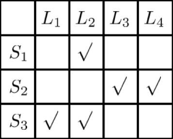
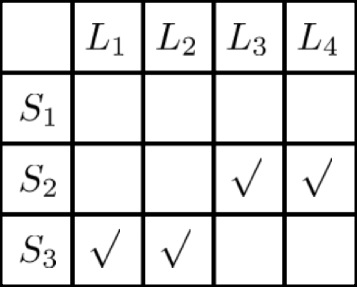
(a) CSCL	(b) NSCL
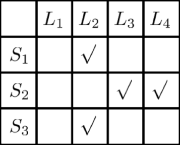
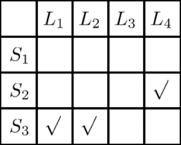
(c) CSNL	(d) NSNL

Figure 1: Assumptions on the cleanness of DS dataset. In each matrix, rows correspond to the sentences in a bag, and columns correspond to the labels assigned to the bag. A check mark on $(S_{i},Lj)$ indicates that the label $L_{j}$ is supported by sentence $S_{i}$.

To the best of our knowledge, this work is the first that combines a neural network model with EM training under the “noisy-sentence noisy-label” assumption. The re-annotated testing dataset , containing the ground-truth relation labels, would also benefit the research community.

2 Problem Statement

Let set ${\mathcal{R}}$ contain all relation labels of interest. Specifically, each label $r$ in ${\mathcal{R}}$ corresponds to a candidate relation in which any considered pair $(e,e^{\prime})$ of entities may participate. Since ${\mathcal{R}}$ cannot contain all relations that are implied in a corpus, we include in ${\mathcal{R}}$ an additional relation label “NA”, which refers to any relation that cannot be regarded as the other relations in ${\mathcal{R}}$.

Any subset of ${\mathcal{R}}$ will be written as a $\{0,1\}$-valued vector of length $|{\mathcal{R}}|$, for example, $z$, where each element of the vector $z$ corresponds to a label $r\in{\mathcal{R}}$. Specifically, if and only if label $r$ is contained in the subset, its corresponding element $z[r]$ of $z$ equals $1$. If two entities $e$ and $e^{\prime}$ participate in a relation $r$, we say that the triple $(e,r,e^{\prime})$ is factual. Let ${\mathcal{B}}$ be a finite set, in which each $b\in{\mathcal{B}}$ is a pair $(e,e^{\prime})$ of entities. Each $b=(e,e^{\prime})\in{\mathcal{B}}$ serves as the index for a bag $x_{b}$ of sentences.

The objective of DS is to use a large but noisy training set to learn a predictor that predicts the relations involving two arbitrary (possibly unseen) entities; the predictor takes as input a bag of sentences each containing the two entities of interest, and hopefully outputs the set of all relations in which the two entities participate.

3 Prior Art and Related Works

Relation extraction is an important task in natural language processing. Many approaches with supervised methods have been proposed to complete this task. These works, such as  Zelenko et al. (2002); Zhou et al. (2005); Bunescu and Mooney (2005), although achieving good performance, rely on carefully selected features and well labelled dataset. Recently, neural network models, have been used in  Zeng et al. (2014); dos Santos et al. (2015); Yang et al. (2016); Liu et al. (2015); Xu et al. (2015); Miwa and Bansal (2016) for supervised relation extraction. These models avoid feature engineering and are shown to improve upon previous models. But having a large number of parameters to estimate, these models rely heavily on costly human-labeled data.

Distant supervision was proposed in  Mintz et al. (2009) to automatically generate large dataset through aligning the given knowledge base to text corpus. However, such dataset can be quite noisy. To articulate the nature of noise in DS dataset, a sentence is said to be noisy if it supports no relation labels of the bag, and a label of the bag is said to be noisy if it is not supported by any sentence in the bag. A sentence or label that is not noisy will be called clean. The cleanness of a training example may obey the following four assumptions, for each of which an example is given In Figure 1.

• Clean-Sentence Clean-Label (CSCL): All sentences and all labels are clean (Figure 1(a)).

• Noisy-Sentence Clean-Label (NSCL): Some sentences may be noisy but all labels are clean (Figure 1(b)). Note that CSCL is a special case of NSCL.

• Clean-Sentence Noisy-Label (CSNL): All sentences are clean but some labels may be noisy(Figure 1(c)). Note that CSNL includes CSCL as a special case.

• Noisy-Sentence Noisy-Label (NSNL): Some sentences may be noisy and some labels may also be noisy (Figure 1(d)).

Obviously, CSCL, NSCL, CSNL are all special cases of NSNL. Thus NSNL is the most general among all these assumptions.

The author of  Mintz et al. (2009) creates a model under the CSCL assumption, which is however pointed out a too strong assumption Riedel et al. (2010). To alleviate this issue, many studies adopt NSCL assumption. Some of them, including  Riedel et al. (2010); Zeng et al. (2015); Lin et al. (2016); Ji et al. (2017); Zeng et al. (2018); Feng et al. (2018); Wang et al. (2018b, a), formulate the task as a multi-instance learning problem where only one label is allowed for each bag. These works take sentence denoising through selecting the max-scored sentence Riedel et al. (2010); Zeng et al. (2015, 2018), applying sentence selection with soft attention Lin et al. (2016); Ji et al. (2017), performing sentence level prediction as well as filtering noisy bags Feng et al. (2018) and redistributing the noisy sentences into negative bags Wang et al. (2018b, a). Other studies complete this task with multi-instance multi-label learning Hoffmann et al. (2011); Surdeanu et al. (2012); Jiang et al. (2016); Ye et al. (2017); Su et al. (2018), which allow overlapping relations in a bag. Despite the demonstrated successes, these models ignore the fact that relation labels can be noisy and “noisy” sentences that indeed point to factual relations may also be ignored. Two recent approaches Liu et al. (2017); Luo et al. (2017) using the NSNL assumption have also been introduced, but these methods are evaluated based on the assumption that the evaluation labels are clean.

We note that this paper is not the first work that combines neural networks with EM training. Very recently, a model also known as Neural Expectation-Maximization or NEM Greff et al. (2017) has been presented to learn latent representations for clusters of objects (e.g., images) under a complete unsupervised setting. The NEM model is not directly applicable to our problem setting which deals with noisy supervision signals from categorical relation labels. Nonetheless, given the existence of the acronym NEM, we choose to abbreviate our Neural Expecation-Maximization model as the nEM model.

4 The nEM Framework

We first introduce the nEM architecture and its learning strategy, and then present approaches to encode a bag of sentences (i.e., the Bag Encoding Models) needed by the framework.

4.1 The nEM Architecture

Let random variable $X$ denote a random bag and random variable $Z$ denote the label set assigned to $X$. Under the NSNL assumption, $Z$, or some labels within, may not be clean for $X$. We introduce another latent random variable $Y$, taking values as a subset of ${\mathcal{R}}$, indicating the set of ground-truth (namely, clean) labels for $X$. We will write $Y$ again as an $|{\mathcal{R}}|$-dimensional $\{0,1\}$-valued vector. From here on, we will adopt the convention that a random variable will be written using a capitalized letter, and the value it takes will be written using the corresponding lower-cased letter.

A key modelling assumption in nEM is that random variables $X$, $Y$ and $Z$ form a Markov chain $X\rightarrow Y\rightarrow Z$. Specifically, the dependency of noisy labels $Z$ on the bag $X$ is modelled as

$$p_{Z|X}(z|x):=\!\!\!\!\!\sum\limits_{y\in\{0,1\}^{|{\mathcal{R}}|}}p_{Y|X}(y|x)p_{Z|Y}(z|y)$$ (1)

The conditional distribution $p_{Z|Y}$ is modelled as

$$p_{Z|Y}(z|y) := \prod\limits_{r\in{\mathcal{R}}}p_{Z[r]|Y[r]}\left(z[r]|y[r]\right)$$ (2)

That is, for each ground-truth label $r\in{\mathcal{R}}$, $Z[r]$ depends only on $Y[r]$. Furthermore, we assume that for each $r$, there are two parameters $\phi_{r}^{0}$ and $\phi_{r}^{1}$ governing the dependency of $Z[r]$ on $Y[r]$ via

$$p_{Z[r]|Y[r]}\!\!\left(\!z[r]|y[r]\right) \!\!\!\!\!\!:=\!\!\!\!\!\! \left\{\begin{array}[]{ll}\!\!\!\!\phi_{r}^{0}&\!\!\!y[r]\!\!=\!0,\!z[r]\!\!=\!1\\ \!\!\!\!1\!\!-\!\phi_{r}^{0}&\!\!\!y[r]\!\!=\!0,\!z[r]\!\!=\!0\\ \!\!\!\!\phi_{r}^{1}&\!\!\!y[r]\!\!=\!1,\!z[r]\!\!=\!0\\ \!\!\!\!1\!\!-\!\phi_{r}^{1}&\!\!\!y[r]\!\!=\!1,\!z[r]\!\!=\!1\end{array}\right.$$ (7)

We will denote by $\{\phi_{r}^{0},\phi_{r}^{1}:r\in{\mathcal{R}}\}$ collectively by $\phi$. .

On the other hand, we model $p_{Y|X}$ by

$$p_{Y|X}(y|x):=\prod\limits_{r\in{\mathcal{R}}}p_{Y[r]|X}\left(y[r]|\overline{x}\right)$$ (8)

where $\overline{x}$ is the encoding of bag $x$, implemented using any suitable neural network. Postponing explaining the details of bag encoding to a later section (namely Section 4.3), we here specify the form of $p_{Y[r]|X}\left(y[r]|\overline{x}\right)$ for each $r$:

$$p_{Y[r]|X}\left(1|\overline{x}\right)=\sigma\left(\overline{r}^{T}\overline{x}+b_{r}\right)$$ (9)

where $\sigma(\cdot)$ is the sigmoid function, $\overline{r}$ is a $|{\mathcal{R}}|$-dimensional vector and $b_{r}$ is bias. That is, $p_{Y[r]|X}$ is essentially a logistic regression (binary) classifier based on the encoding $\overline{x}$ of bag $x$. We will denote by $\theta$ the set of all parameters $\{\overline{r}:r\in{\mathcal{R}}\}$ and the parameters for generating encoding $\overline{x}$.

At this end, we have defined the overall structure of the nEM framework (summarized in Figure 2). Next, we will discuss the learning of it.

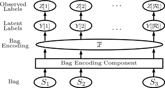
Figure 2: The probabilistic framework of nEM

4.2 Learning with the EM Algorithm

Let $\ell(z|x;\phi,\theta)$ be the log-likelihood of observing the label set $z$ given the bag $x$, that is,

$$\ell(z|x;\phi,\theta):=\log p_{Z|X}(z|x).$$ (10)

The structure of the framework readily enables a principled learning algorithm based on the EM algorithm Dempster et al. (1977).

Let $\ell_{\rm total}(\phi,\theta)$ be the log-likelihood defined as

$$\ell_{\rm total}(\phi,\theta) := \sum_{b\in{\mathcal{B}}}\ell(z_{b}|x_{b};\phi,\theta).$$ (11)

The learning problem can then be formulated as maximizing this objective function over its parameters $(\phi,\theta)$, or solving

$$(\widehat{\phi},\widehat{\theta}):=\arg\max_{\phi,\theta}\ell_{\rm total}(\phi,\theta).$$ (12)

Let $Q$ be an arbitrary distribution over $\{0,1\}^{|{\mathcal{R}}|}$. Then it is possible to show

$$\begin{split}&\ell(z|x;\phi,\theta)\\ &\!\!\!=\!\log\!\!\!\!\!\!\sum\limits_{y\in\{0,1\}^{|{\mathcal{R}}|}}\!\!\!\!\!\!Q(y)\frac{\prod\limits_{r\in{\mathcal{R}}}\!\!p_{Y[r]|X}(y[r]|\overline{x})p_{Z[r]|Y[r]}(z[r]|y[r])}{Q(y)}\\ &\!\!\!\geqslant\!\!\!\!\!\!\!\sum\limits_{y\in\{0,1\}^{|{\mathcal{R}}|}}\!\!\!\!\!\!\!Q(y)\log\!\frac{\prod\limits_{r\in{\mathcal{R}}}\!\!p_{Y[r]|X}(y[r]|\overline{x})p_{Z[r]|Y[r]}(z[r]|y[r])}{Q(y)}\\ &\!\!\!={\mathcal{L}}(z|x;\phi,\theta,Q)\end{split}$$ (13)

where the lower bound ${\mathcal{L}}(z|x;\phi,\theta,Q)$, often referred to as the variational lower bound. Now we define ${\mathcal{L}}_{\rm total}$ as

$${\mathcal{L}}_{\rm total}(\!\phi,\!\theta,\!\{Q_{b}\!:\!b\!\in\!{\mathcal{B}}\}\!)\!\!:=\!\!\!\sum\limits_{b\in{\mathcal{B}}}\!\!{\mathcal{L}}\left(z_{b}|x_{b};\!\phi,\!\theta,\!Q_{b}\right)$$ (14)

where we have introduced a $Q_{b}$ for each $b\in{\mathcal{B}}$. Instead of solving the original optimization problem (12), we can turn to solving a different optimization problem by maximizing ${\mathcal{L}}_{\rm total}$

$$\begin{split}\!\!\!(\widehat{\phi},\widehat{\theta},\{\widehat{Q}_{b}\})\!:=\!\arg\!\!\!\max_{\phi,\theta,\{Q_{b}\}}\!\!{\mathcal{L}}_{\rm total}(\phi,\theta,\{Q_{b}\})\end{split}$$ (15)

The EM algorithm for solving the optimization problem (15) is essentially the coordinate ascent algorithm on objective function ${\mathcal{L}}_{\rm total}$, where we iterate over two steps, the E-Step and the M-Step. In the E-Step, we maximizes ${\mathcal{L}}_{\rm total}$ over $\{Q_{b}\}$ for the current setting of $(\phi,\theta)$ and in the M-Step, we maximize ${\mathcal{L}}_{\rm total}$ $(\phi,\theta)$ for the current setting of $\{Q_{b}\}$. We now describe the two steps in detail, where we will use superscript $t$ to denote the iteration number.

E-step: In this step, we hold $(\phi,\theta)$ fixed and update $\{Q_{b}:b\in{\mathcal{B}}\}$ to maximize the lower bound $\mathcal{L}_{\rm total}(\phi,\theta,\{Q_{b}\})$. This boils down to update each factor $Q_{b,r}$ of $Q_{b}$ according to:

$$\begin{split}\!\!\!\!Q_{b,r}^{t+1}(y[r])\!:&\!=\!p_{Y[r]|X,Z}(y_{b}[r]|x_{b},z_{b}[r];\theta^{t},\phi_{r}^{t})\\ &=\!\frac{p_{Z|Y}(z_{b}[r]|y_{b}[r];\phi_{r}^{t})p_{Y|X}(y_{b}[r]|x_{b};\theta^{t})}{p_{Z|X}(z_{b}[r]|x_{b};\theta^{t},\phi_{r}^{t})}\\ &=\!\frac{p_{Z|Y}(z_{b}[r]|y_{b}[r];\phi_{r}^{t})p_{Y|X}(y_{b}[r]|x_{b};\theta^{t})}{\!\!\!\!\!\!\!\!\sum\limits_{y[r]\in\left\{0,1\right\}}\!\!\!\!\!\!\!p_{Z|Y}(z_{b}[r]|y[r];\phi_{r}^{t})p_{Y|X}(y[r]|x_{b};\theta^{t})}\end{split}$$ (16)

M-step: In this step, we hold $\{Q_{b}\}$ fixed and update $(\phi,\theta)$, to maximize the lower bound $\mathcal{L}_{\rm total}(\phi,\theta,\{Q_{b}\})$. Let

$$\begin{split}M=\prod\limits_{r\in{\mathcal{R}}}\!\!p_{Y[r]|X}(y_{b}[r]|\overline{x}_{b})p_{Z[r]|Y[r]}(z_{b}[r]|y_{b}[r]),\end{split}$$ (17)

then $(\phi,\theta)$ is updated according to:

$$\begin{split}&(\theta^{t+1},\phi^{t+1}):=\arg\!\max_{\theta,\phi}\mathcal{L}_{\rm total}(\theta,\phi,\{Q_{b}^{t+1}\})\\ &\!\!\!=\!\arg\!\max_{\theta,\phi}\!\!\!\sum\limits_{b\in{\mathcal{B}}}\!\sum\limits_{y_{b}\in\{0,1\}^{|{\mathcal{R}}|}}\!\!\!\!\!\!\!\!\!\!Q_{b}^{t+1}(y)\!\log\frac{M}{Q_{b}^{t+1}(y)}\\ &\!\!\!=\!\arg\!\max_{\theta,\phi}\!\!\!\sum\limits_{b\in{\mathcal{B}}}\!\sum\limits_{y_{b}\!\in\!\{\!0,\!1\!\}^{\!|\!{\mathcal{R}}\!|}}\!\!\!\!\!\!\!\!Q_{\!b}^{t\!+\!1}\!(y)\!\log\!M\!\!-\!\!\!\!\sum\limits_{\!\!b\!\in{\mathcal{B}}}\!\!\sum\limits_{y_{b}\!\in\!\left\{\!0,\!1\!\right\}^{\!|\!{\mathcal{R}}\!|}}\!\!\!\!\!\!\!\!Q_{b}^{t}(y)\!\log\!Q_{b}^{t+1}(y)\\ &\!\!\!=\!\arg\!\max_{\theta,\phi}\!\!\!\sum\limits_{b\in{\mathcal{B}}}\!\sum\limits_{r\in{\mathcal{R}}}\!\sum\limits_{y_{b}\![\!r\!]\in\!\left\{\!0,\!1\!\right\}}\!\!\!\!\!\!\!Q_{\!b,r}^{t+1}\!(y[r])\!\left(\log p_{Z|Y}(z_{b}[r]|y_{b}[r];\phi_{r})\right.\\ &\phantom{=\;\;}\left.\!+\log p_{Y|X}(y_{b}[r]|\overline{x}_{b};\theta)\right)\end{split}$$ (18)

Overall the EM algorithm starts with initializing $(\phi,\theta,\{Q_{b}\})$, and then iterates over the two steps until convergence or after some prescribed number of iterations is reached. There are however several caveats on which caution is needed. First, the optimization problem in the M-Step cannot be solved in closed form. As such we take a stochastic gradient descent (SGD) approach.

In each M-Step, we perform $\Delta$ updates, where $\Delta$ is a hyper-parameter. Such an approach is sometimes referred to as “Generalized EM”  Wu (1983); Jojic and Frey (2001); Greff et al. (2017). Note that since the parameters $\theta$ are parameters for the neural network performing bag encoding, the objective function ${\mathcal{L}}_{\rm total}$ is highly non-convex with respect to $\theta$. This makes it desirable to choose an appropriate $\Delta$. Too small $\Delta$ results in little change in $\theta$ and hence provides insufficient signal to update $\{Q_{b}\}$; too large $\Delta$, particularly at the early iterations when $\{Q_{b}\}$ has not been sufficiently optimized, tends to make the optimization stuck in undesired local optimum. In practice, one can try several values of $\Delta$ by inspecting their achieved value of ${\mathcal{L}}_{\rm total}$ and select the $\Delta$ giving rise to the highest ${\mathcal{L}}_{\rm total}$. Note that such a tuning of $\Delta$ requires no access of the testing data. The second issue is that the EM algorithm is known to be sensitive to initialization. In our implementation, in order to provide a good initial parameter setting, we set each $Q_{b}^{0}$ to $z_{b}$. Despite the fact that $z$ contains noise, this is a much better approximation of the posterior of true labels than any random initialization.

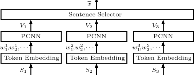
Figure 3: The structure of Bag Encoding component.

The nEM framework needs the encoding of a bag of $x$ as discussed in Equation 8. Any suitable neural network can be deployed to achieve this goal. Next, we present the widely used methods for DS relation extraction strategies: the Bag Encoding Models.

4.3 Bag Encoding Models

As illustrated in Figure 3, the Bag Encoding Models include three components: Word-Position Embedding, Sentence Encoding, and Sentence Selectors.

4.3.1 Word-Position Embedding

For the $j^{\rm th}$ word in a sentence, Word-Position Embedding generates a vector representation ${\bf w}_{j}$ as concatenated three components $\left[{\bf w}_{j}^{w},{\bf w}_{j}^{p1},{\bf w}_{j}^{p2}\right]$. Specifically, ${\bf w}_{j}^{w}$ is the word embedding of the word and ${\bf w}_{j}^{p1}$ and ${\bf w}_{j}^{p2}$ are two position embeddings. Here ${\bf w}_{j}^{p1}$ (resp. ${\bf w}_{j}^{p2}$) are the embedding of the relative location of the word with respect to the first (resp. second) entity in the sentence. The dimensions of word and position embeddings are denoted by $d_{w}$ and $d_{p}$ respectively.

4.3.2 Sentence Encoding

Sentence encoding uses Piecewise Convolutional Neural Networks (PCNN) Zeng et al. (2015); Lin et al. (2016); Ye et al. (2017); Ji et al. (2017), which consists of convolution followed by Piecewise Max-pooling. The convolution operation uses a list of matrix kernels such as $\left\{{\bf K}_{1},{\bf K}_{2},\cdots,{\bf K}_{l_{ker}}\right\}$ to extract n-gram features through sliding windows of length $l_{win}$. Here ${\bf K}_{i}\in\mathbb{R}^{l_{win}\times d_{e}}$ and $l_{ker}$ is the number of kernels. Let ${\bf w}_{j-l_{win}+1:j}\in\mathbb{R}^{l_{win}\times d_{e}}$ be the concatenated vector of token embeddings in the $j^{\rm th}$ window. The output of convolution operation is a matrix ${\bf U}\in\mathbb{R}^{l_{ker}\times(m+l_{win}-1)}$ where each element is computed by

$${\bf U}_{ij}={\bf K}_{i}\odot{\bf w}_{j-l_{win}+1:j}+b_{i}$$ (19)

where $\odot$ denotes inner product. In Piecewise Max-Pooling, ${\bf U}_{i}$ is segmented to three parts $\left\{{\bf U}_{i}^{1},{\bf U}_{i}^{2},{\bf U}_{i}^{3}\right\}$ depending on whether an element in ${\bf U}_{i}$ is on the left or right of the two entities, or between the two entities. Then max-pooling is applied to each segment, giving rise to

$${\bf g}^{ip}=\max({\bf U}_{i}^{p}),1\leqslant i\leqslant l_{ker},1\leqslant p\leqslant 3$$ (20)

Let ${\bf g}=\left[{\bf g}^{1},{\bf g}^{2},{\bf g}^{3}\right]$. Then sentence encoding outputs

$${\bf v}={\rm ReLU}({\bf g})\circ{\bf h},$$ (21)

where $\circ$ is element-wise multiplication and ${\bf h}$ is a vector of Bernoulli random variables, representing dropouts.

4.3.3 Sentence Selectors

Let $n$ be the number of sentences in a bag. We denote a matrix ${\bf V}\in\mathbb{R}^{n\times(l_{ker}\times 3)}$consisting of each sentence vector ${\bf v}_{T}$. ${\bf V}_{k:}$ and ${\bf V}_{:j}$ are used to index the $k^{\rm th}$ row vector and $j^{\rm th}$ column vector of ${\bf V}$ respectively. Three kinds of sentence-selectors are used to construct the bag encoding. Mean-selector Lin et al. (2016); Ye et al. (2017): The bag encoding is computed as

$$\overline{x}=\frac{1}{n}\sum_{k=1}^{n}{\bf V}_{k:}$$ (22)

Max-selector Jiang et al. (2016): The $j^{\rm th}$ element of bag encoding $\overline{x}$ is computed as

$$\overline{x}_{j}=\max({\bf V}_{:j})$$ (23)

Attention-selector Attention mechanism is extensively used for sentence selection in relation extraction by weighted summing of the sentence vectors, such as in  Lin et al. (2016); Ye et al. (2017); Su et al. (2018). However, all these works assume that the labels are correct and only use the golden label embeddings to select sentences at training stage. We instead selecting sentences using all label embeddings $\overline{r}$ and construct a bag encoding for each label $r\in{\mathcal{R}}$. The output is then a list of vectors $\left\{\overline{x}^{r}\right\}$, in which the $r^{\rm th}$ vector is calculated through attention mechanism as

$$e_{l}\!\!=\!\!{\bf V}_{\!l:}^{\!T}\!{\bf A}\overline{r},~{}\alpha_{k}\!\!=\!\!\frac{\exp(e_{k})}{\sum_{l=\!1}^{n}\!\exp(e_{l})},~{}\overline{x}^{r}\!\!\!=\!\!\!\sum_{k=1}^{n}\!\!\alpha_{k}\!\!{\bf V}_{\!\!k:}$$ (24)

where ${\bf A}\in\mathbb{R}^{d_{r}\times d_{r}}$ is a diagonal matrix and $d_{r}$ is the dimension of relation embedding.

5 Experimental Study

We first conduct experiments on the widely used benchmark data set Riedel Riedel et al. (2010), and then on the TARCED Zhang et al. (2017) data set. The latter allows us to control the noise level in the labels to observe the behavior and working mechanism of our proposed method. The code for our model is found on the Github page .

5.1 Evaluation on the Riedel Dataset

The Riedel dataset is a widely used DS dataset for relation extraction. It was developed in  Riedel et al. (2010) through aligning entity pairs from Freebase with the New York Times (NYT) corpus. There are 53 relations in the Riedel dataset, including “NA”. The bags collected from the 2005-2006 corpus are used as the training set, and the bags from the 2007 corpus are used as the test set. The training data contains $281,270$ entity pairs and $522,611$ sentences; the testing data contains $96,678$ entity pairs and $172,448$ sentences.

5.1.1 Ground-Truth Annotation

The Riedel dataset contains no ground-truth labels. The held-out evaluation Mintz et al. (2009) is highly unreliable in measuring a model’s performance against the ground truth. Since this study is concerned with discovering the ground-truth labels, the conventional held-out evaluation is no longer appropriate. For this reason, we annotate a subset of the original test data for evaluation purpose. Specifically, we annotate a bag $x_{b}$ by its all correct labels, and if no such labels exist, we label the bag NA.

In total 3762 bags are annotated, which include all bags originally labelled as non-NA (”Part 1”) and 2000 bags (”Part 2”) selected from the bags originally labelled as NA but have relatively low score for NA label under a pre-trained PCNN+ATT Lin et al. (2016) model. The rationale here is that we are interested in inspecting the model’s performance in detecting the labels of known relations rather than NA relation.

Table 1: The statistics of ground-truth annotation. origin denotes the total number of originally assigned labels of these bags. correct and wrong denote the total number of correctly assigned and wrongly assigned labels. added denote the number of missing labels we added into these bags.

	bags	origin	correct	wrong	added
Part 1	1762	1953	1245	708	804
Part 2	2000	2000	938	1062	1211

The statistics of annotation is shown in Table  1. Through the annotation, we notice that, about 36% of the original labels in original non-NA bags and 53% of labels in original NA bags are wrongly assigned. Similar statistics has been reported in previous works  Riedel et al. (2010); Feng et al. (2018).

5.1.2 Evaluation Metrics and Baselines

For the Riedel dataset, we train the models on the noisy training set and test the models on the manually labeled test set. The precision-recall (PR) curve is reported to compare performance of models. Three baselines are considered:

• PCNN+MEAN Lin et al. (2016); Ye et al. (2017): A model using PCNN to encode sentences and a mean-selector to generate bag encoding.

• PCNN+MAX Jiang et al. (2016): A model using PCNN to encode sentences and a max-selector to generate bag encoding.

• PCNN+ATT Lin et al. (2016); Ye et al. (2017); Su et al. (2018): A model using PCNN to encode sentences and an attention-selector to generate bag encoding.

We compare the three baselines with their nEM versions (namely using them as the Bag Encoding component in nEM), which are denoted with a “+nEM” suffix.

5.1.3 Implementation Detail

Following previous work, we tune our models using three-fold validation on the training set. As the best configurations, we set $d_{w}=50$, $d_{p}=5$ and $d_{r}=230$. For PCNN, we set $l_{win}=3$, $l_{ker}=230$ and set the probability of dropout to $0.5$. We use Adadelta Zeiler (2012) with default setting ($\rho=0.95,\varepsilon=1e^{-6}$) to optimize the models and the initial learning rate is set as $1$. The batch size is fixed to $160$ and the max length of a sentence is set as $120$.

For the noise model $p_{Z\mid Y}$, we set $\phi_{NA}^{0}=0.3,\phi_{NA}^{1}=0$ for the NA label and $\phi_{r}^{0}=0,\phi_{r}^{1}=0.9$ for other labels $r\neq NA$. In addition, the number $\Delta$ of SGD updates in M-step is set to $2000$.

5.1.4 Predictive performance

The evaluation results on manually labeled test set are shown in Figure  4. From which, we observe that the PR-curves of the nEM models are above their corresponding baselines by significant margins, especially in the low-recall regime. This observation demonstrates the effectiveness of the nEM model on improving the extracting performance upon the baseline models.

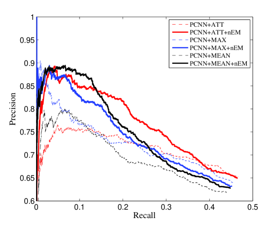
Figure 4: PR curves on DS test set.

We also observe that models with attention-selector achieve better performance than models with mean-selector and max-selector, demonstrating the superiority of the attention mechanism on sentence selection.

We then analyze the predicting probability of PCNN+ATT and PCNN+ATT+nEM on the ground-truth labels in the test set. We divide the predicting probability values into $5$ bins and count the number of label within each bin. The result is shown in Figure  5(a). We observe that the count for PCNN+ATT in bins $0.0-0.2$, $0.2-0.4$, $0.4-0.6$ and $0.6-0.8$ are all greater than PCNN+ATT+nEM. But in bin $0.8-1.0$, the count for PCNN+ATT+nEM is about 55% larger than PCNN+ATT. This observation indicates that nEM can promote the overall predicting scores of ground-truth labels.

Figure  5(b) compares PCNN+ATT and PCNN+ATT+nEM in their predictive probabilities on the frequent relations. The result shows that PCNN+ATT+nEM achieves higher average predicting probability on all these relations, except for the NA relation, on which PCNN+ATT+nEM nearly levels with PCNN+ATT. This phenomenon demonstrates that nEM tends to be more confident in predicting the correct labels. In this case, raising the predictive probability on the correct label does increase the model’s ability to make the correct decision, thereby improving performance.

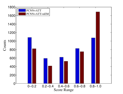
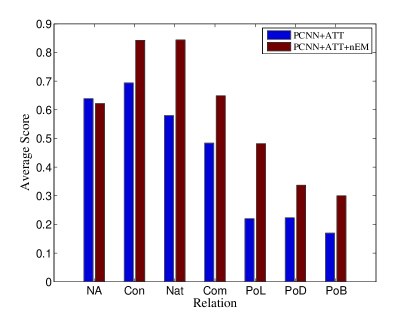
(a) Score distribution	(b) Scores on main relations

Figure 5: Predictive probabilities on the test set. CON, Nat, Com, PoL, PoD and PoB represent ’contains’, ’nationality’, ’company’, ’place lived’, ’place of death’ and ’place of birth’ relations respectively.

5.2 Evaluation on the TACRED Dataset

TACRED is a large supervised relation extraction dataset collected in  Zhang et al. (2017). The text corpus is generated from the TAC KBP evaluation of years $2009-2015$. Corpus from years $2009-2012$, year $2013$ and year $2014$ are used as training, validation and testing sets respectively. In all annotated sentences, $68,124$ are used for training, $22,631$ for validation and $15,509$ for testing. There are in total $42,394$ distinct entity pairs, where $33,079$ of these entity pairs appear in exactly one sentence. Since these $33,079$ entity pairs dominate the training set, we simply treat each sentence as a bag for training and testing. Another advantage of constructing single-sentence bags is that it allows us to pinpoint the correspondence between the correct label and its supporting sentence. The number of relations in TACRED dataset is $42$, including a special relation “no relation”, which is treated as NA in this study.

5.2.1 Constructing Semi-synthetic Dataset

To obtain insight into the working of nEM, we create a simulated DS dataset by inserting noisy labels into the training set of a supervised dataset, TACRED. Since the training set of TACRED was manually annotated, the labels therein may be regarded as the ground-truth labels. Training using this semi-synthetic dataset allows us to easily observe models’ behaviour with respect to the noisy labels and the true labels.

We inject artificial noise into the TACRED training data through the following precedure. For each bag $x_{b}$ in the training set, we generate a noisy label vector $\tilde{z}_{b}$ from the observed ground-truth label vector $y_{b}$. Specifically, $\tilde{z}_{b}$ is generated by flipping each element $y_{b}[r]$ from $0$ to $1$ or $1$ to $0$ with a probability $p_{f}$. This precedure simulates a DS dataset through introducing wrong labels into training bags, thus corrupts the training dataset.

5.2.2 Experimental Settings

Following  Zhang et al. (2017), the common relation classification metrics Precision, Recall and F1 are used for evaluation. The PCNN model is used to generate the bag encoding since sentence selection is not needed in this setting. The same hyper-parameter settings as in Section  5.1.3 are used in this experiment. For the noise model $p_{Z[r]|Y[r]}$ of PCNN +nEM, we set $\phi_{r}^{0}=0.1,\phi_{r}^{1}=0.1$ for each label $r\in{\mathcal{R}}$. The number $\Delta$ of SGD updates in each M-step is set to $1600$.

5.2.3 Test Results

From Table  2, we see that PCNN+nEM achieves better recall and F1 score than the PCNN model under various noise levels. Additionally, the recall and F1 margins between PCNN and PCNN+nEM increase with noise levels. This suggests that nEM keeps better performance than the corresponding baseline model under various level of training noise. We also observe that the precision of nEM is consistently lower than that of PCNN when noise is injected to TACRED. This is a necessary trade-off present in nEM. The training of nEM regards the training labels with less confidence based on noisy-label assumption. This effectively lowers the probability of seen training labels and considers the unseen labels also having some probability to occur. When trained this way, nEM, at the prediction time, tends to predict more labels than its baseline (PCNN) does. Note that in TACRED, each instance contains only a single ground truth label. Thus the tendency of nEM to predict more labels leads to the reduced precision. However, despite this tendency, nEM, comparing with PCNN, has a stronger capability in detecting the correct label and gives the better recall of nEM. The gain in recall dominates the loss in precision.

Table 2: Test performance on the TACRED dataset.

$p_{f}$	PCNN			PCNN+nEM
	P	R	F1	P	R	F1
0.02	65.2	30.0	41.1	61.8	34.8	44.5
0.04	63.5	28.9	39.7	60.2	33.8	43.3
0.06	70.5	25.2	37.1	59.9	31.1	41.0
0.08	63.5	23.6	34.4	58.8	29.8	39.6
0.10	66.1	22.7	33.9	56.5	28.9	38.3

5.2.4 Training Label Probabilities

The predicting probabilities for the noise labels and the original true labels are also evaluated under the trained models. The results are shown in Figure  6 (left) which reveals that with increasing noise, the average probability for noisy label sets of PCNN and PCNN+nEM both increase and average scores for original label sets of PCNN and PCNN+nEM both decrease. The performance degradation of PCNN and PCNN+nEM under noise appears different. The average probability for noisy label sets rises with a higher slope in PCNN than in PCNN+nEM. Additionally, the average probability for the original label sets of PCNN+nEM is higher than or equal to PCNN at all noise levels. These observations confirms that the denoising capability of nEM is learned from effectively denoising the training set.

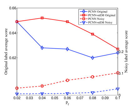
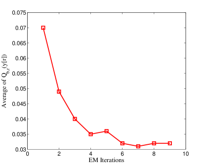
Figure 6: Average probabilities for noisy and original labels (left) and average $Q_{b,r}(y[r])$ over EM iterations (right)

5.2.5 Effectiveness of EM Iterations

For each training bag $x_{b}$ and each artificial noisy label $r$, we track the probability $Q_{b,r}(y[r])=1$ over EM iterations. This probability, measuring the likelihood of the noise label $r$ being correct, is then averaged over $r$ and over all bags $x_{b}$. It can be seen in Figure  6 (right) that the average value of $Q_{b,r}(y[r])$ decreases as the training progresses, leading the model to gradually ignore noisy labels. This demonstrates the effectiveness of EM iterations and validates the proposed EM-based framework.

6 Concluding Remarks

We proposed a nEM framework to deal with the noisy-label problem in distance supervision relation extraction. We empirically demonstrated the effectiveness of the nEM framework, and provided insights on its working and behaviours through data with controllable noise levels. Our framework is a combination of latent variable models in probabilistic modelling with contemporary deep neural networks. Consequently, it naturally supports a training algorithm which elegantly nests the SGD training of any appropriate neural network inside an EM algorithm. We hope that our approach and the annotated clean testing data would inspire further research along this direction.

References

- Bunescu and Mooney (2005) Razvan C. Bunescu and Raymond J. Mooney. 2005. Subsequence kernels for relation extraction. In Advances in Neural Information Processing Systems 18 [Neural Information Processing Systems, NIPS 2005, December 5-8, 2005, Vancouver, British Columbia, Canada], pages 171–178.
- Dempster et al. (1977) Arthur P Dempster, Nan M Laird, and Donald B Rubin. 1977. Maximum likelihood from incomplete data via the em algorithm. Journal of the royal statistical society. Series B (methodological), pages 1–38.
- Feng et al. (2018) Jun Feng, Minlie Huang, Li Zhao, Yang Yang, and Xiaoyan Zhu. 2018. Reinforcement learning for relation classification from noisy data. In Proceedings of the Thirty-Second AAAI Conference on Artificial Intelligence, (AAAI-18), the 30th innovative Applications of Artificial Intelligence (IAAI-18), and the 8th AAAI Symposium on Educational Advances in Artificial Intelligence (EAAI-18), New Orleans, Louisiana, USA, February 2-7, 2018, pages 5779–5786.
- Gábor et al. (2018) Kata Gábor, Davide Buscaldi, Anne-Kathrin Schumann, Behrang QasemiZadeh, Haïfa Zargayouna, and Thierry Charnois. 2018. Semeval-2018 task 7: Semantic relation extraction and classification in scientific papers. In SemEval@NAACL-HLT, pages 679–688. Association for Computational Linguistics.
- Greff et al. (2017) Klaus Greff, Sjoerd van Steenkiste, and Jürgen Schmidhuber. 2017. Neural expectation maximization. In Advances in Neural Information Processing Systems 30: Annual Conference on Neural Information Processing Systems 2017, 4-9 December 2017, Long Beach, CA, USA, pages 6694–6704.
- Hoffmann et al. (2011) Raphael Hoffmann, Congle Zhang, Xiao Ling, Luke S. Zettlemoyer, and Daniel S. Weld. 2011. Knowledge-based weak supervision for information extraction of overlapping relations. In The 49th Annual Meeting of the Association for Computational Linguistics: Human Language Technologies, Proceedings of the Conference, 19-24 June, 2011, Portland, Oregon, USA, pages 541–550.
- Ji et al. (2017) Guoliang Ji, Kang Liu, Shizhu He, and Jun Zhao. 2017. Distant supervision for relation extraction with sentence-level attention and entity descriptions. In Proceedings of the Thirty-First AAAI Conference on Artificial Intelligence, February 4-9, 2017, San Francisco, California, USA., pages 3060–3066.
- Jiang et al. (2016) Xiaotian Jiang, Quan Wang, Peng Li, and Bin Wang. 2016. Relation extraction with multi-instance multi-label convolutional neural networks. In COLING 2016, 26th International Conference on Computational Linguistics, Proceedings of the Conference: Technical Papers, December 11-16, 2016, Osaka, Japan, pages 1471–1480.
- Jojic and Frey (2001) Nebojsa Jojic and Brendan J. Frey. 2001. Learning flexible sprites in video layers. In 2001 IEEE Computer Society Conference on Computer Vision and Pattern Recognition (CVPR 2001), with CD-ROM, 8-14 December 2001, Kauai, HI, USA, pages 199–206.
- Lin et al. (2016) Yankai Lin, Shiqi Shen, Zhiyuan Liu, Huanbo Luan, and Maosong Sun. 2016. Neural relation extraction with selective attention over instances. In Proceedings of the 54th Annual Meeting of the Association for Computational Linguistics, ACL 2016, August 7-12, 2016, Berlin, Germany, Volume 1: Long Papers.
- Liu et al. (2017) Tianyu Liu, Kexiang Wang, Baobao Chang, and Zhifang Sui. 2017. A soft-label method for noise-tolerant distantly supervised relation extraction. In Proceedings of the 2017 Conference on Empirical Methods in Natural Language Processing, EMNLP 2017, Copenhagen, Denmark, September 9-11, 2017, pages 1790–1795.
- Liu et al. (2015) Yang Liu, Furu Wei, Sujian Li, Heng Ji, Ming Zhou, and Houfeng Wang. 2015. A dependency-based neural network for relation classification. In Proceedings of the 53rd Annual Meeting of the Association for Computational Linguistics and the 7th International Joint Conference on Natural Language Processing of the Asian Federation of Natural Language Processing, ACL 2015, July 26-31, 2015, Beijing, China, Volume 2: Short Papers, pages 285–290.
- Luo et al. (2017) Bingfeng Luo, Yansong Feng, Zheng Wang, Zhanxing Zhu, Songfang Huang, Rui Yan, and Dongyan Zhao. 2017. Learning with noise: Enhance distantly supervised relation extraction with dynamic transition matrix. In Proceedings of the 55th Annual Meeting of the Association for Computational Linguistics, ACL 2017, Vancouver, Canada, July 30 - August 4, Volume 1: Long Papers, pages 430–439.
- Mintz et al. (2009) Mike Mintz, Steven Bills, Rion Snow, and Daniel Jurafsky. 2009. Distant supervision for relation extraction without labeled data. In ACL 2009, Proceedings of the 47th Annual Meeting of the Association for Computational Linguistics and the 4th International Joint Conference on Natural Language Processing of the AFNLP, 2-7 August 2009, Singapore, pages 1003–1011.
- Miwa and Bansal (2016) Makoto Miwa and Mohit Bansal. 2016. End-to-end relation extraction using lstms on sequences and tree structures. In Proceedings of the 54th Annual Meeting of the Association for Computational Linguistics, ACL 2016, August 7-12, 2016, Berlin, Germany, Volume 1: Long Papers.
- Qu et al. (2018) Meng Qu, Xiang Ren, Yu Zhang, and Jiawei Han. 2018. Weakly-supervised relation extraction by pattern-enhanced embedding learning. In Proceedings of the 2018 World Wide Web Conference on World Wide Web, WWW 2018, Lyon, France, April 23-27, 2018, pages 1257–1266.
- Riedel et al. (2010) Sebastian Riedel, Limin Yao, and Andrew McCallum. 2010. Modeling relations and their mentions without labeled text. In Machine Learning and Knowledge Discovery in Databases, European Conference, ECML PKDD 2010, Barcelona, Spain, September 20-24, 2010, Proceedings, Part III, pages 148–163.
- dos Santos et al. (2015) Cícero Nogueira dos Santos, Bing Xiang, and Bowen Zhou. 2015. Classifying relations by ranking with convolutional neural networks. In Proceedings of the 53rd Annual Meeting of the Association for Computational Linguistics and the 7th International Joint Conference on Natural Language Processing of the Asian Federation of Natural Language Processing, ACL 2015, July 26-31, 2015, Beijing, China, Volume 1: Long Papers, pages 626–634.
- Su et al. (2018) Sen Su, Ningning Jia, Xiang Cheng, Shuguang Zhu, and Ruiping Li. 2018. Exploring encoder-decoder model for distant supervised relation extraction. In Proceedings of the Twenty-Seventh International Joint Conference on Artificial Intelligence, IJCAI 2018, July 13-19, 2018, Stockholm, Sweden., pages 4389–4395.
- Surdeanu et al. (2012) Mihai Surdeanu, Julie Tibshirani, Ramesh Nallapati, and Christopher D. Manning. 2012. Multi-instance multi-label learning for relation extraction. In Proceedings of the 2012 Joint Conference on Empirical Methods in Natural Language Processing and Computational Natural Language Learning, EMNLP-CoNLL 2012, July 12-14, 2012, Jeju Island, Korea, pages 455–465.
- Wang et al. (2018a) William Yang Wang, Weiran Xu, and Pengda Qin. 2018a. DSGAN: generative adversarial training for distant supervision relation extraction. In Proceedings of the 56th Annual Meeting of the Association for Computational Linguistics, ACL 2018, Melbourne, Australia, July 15-20, 2018, Volume 1: Long Papers, pages 496–505.
- Wang et al. (2018b) William Yang Wang, Weiran Xu, and Pengda Qin. 2018b. Robust distant supervision relation extraction via deep reinforcement learning. In Proceedings of the 56th Annual Meeting of the Association for Computational Linguistics, ACL 2018, Melbourne, Australia, July 15-20, 2018, Volume 1: Long Papers, pages 2137–2147.
- Wu (1983) CF Jeff Wu. 1983. On the convergence properties of the em algorithm. The Annals of statistics, pages 95–103.
- Xu et al. (2015) Yan Xu, Lili Mou, Ge Li, Yunchuan Chen, Hao Peng, and Zhi Jin. 2015. Classifying relations via long short term memory networks along shortest dependency paths. In Proceedings of the 2015 Conference on Empirical Methods in Natural Language Processing, EMNLP 2015, Lisbon, Portugal, September 17-21, 2015, pages 1785–1794.
- Yang et al. (2016) Yunlun Yang, Yunhai Tong, Shulei Ma, and Zhi-Hong Deng. 2016. A position encoding convolutional neural network based on dependency tree for relation classification. In Proceedings of the 2016 Conference on Empirical Methods in Natural Language Processing, EMNLP 2016, Austin, Texas, USA, November 1-4, 2016, pages 65–74.
- Ye et al. (2017) Hai Ye, Wenhan Chao, Zhunchen Luo, and Zhoujun Li. 2017. Jointly extracting relations with class ties via effective deep ranking. In Proceedings of the 55th Annual Meeting of the Association for Computational Linguistics, ACL 2017, Vancouver, Canada, July 30 - August 4, Volume 1: Long Papers, pages 1810–1820.
- Zeiler (2012) Matthew D. Zeiler. 2012. ADADELTA: an adaptive learning rate method. CoRR, abs/1212.5701.
- Zelenko et al. (2002) Dmitry Zelenko, Chinatsu Aone, and Anthony Richardella. 2002. Kernel methods for relation extraction. In Proceedings of the 2002 Conference on Empirical Methods in Natural Language Processing, EMNLP 2002, Philadelphia, PA, USA, July 6-7, 2002.
- Zeng et al. (2015) Daojian Zeng, Kang Liu, Yubo Chen, and Jun Zhao. 2015. Distant supervision for relation extraction via piecewise convolutional neural networks. In Proceedings of the 2015 Conference on Empirical Methods in Natural Language Processing, EMNLP 2015, Lisbon, Portugal, September 17-21, 2015, pages 1753–1762.
- Zeng et al. (2014) Daojian Zeng, Kang Liu, Siwei Lai, Guangyou Zhou, and Jun Zhao. 2014. Relation classification via convolutional deep neural network. In COLING 2014, 25th International Conference on Computational Linguistics, Proceedings of the Conference: Technical Papers, August 23-29, 2014, Dublin, Ireland, pages 2335–2344.
- Zeng et al. (2018) Xiangrong Zeng, Shizhu He, Kang Liu, and Jun Zhao. 2018. Large scaled relation extraction with reinforcement learning. In Proceedings of the Thirty-Second AAAI Conference on Artificial Intelligence, (AAAI-18), the 30th innovative Applications of Artificial Intelligence (IAAI-18), and the 8th AAAI Symposium on Educational Advances in Artificial Intelligence (EAAI-18), New Orleans, Louisiana, USA, February 2-7, 2018, pages 5658–5665.
- Zhang et al. (2017) Yuhao Zhang, Victor Zhong, Danqi Chen, Gabor Angeli, and Christopher D. Manning. 2017. Position-aware attention and supervised data improve slot filling. In Proceedings of the 2017 Conference on Empirical Methods in Natural Language Processing, EMNLP 2017, Copenhagen, Denmark, September 9-11, 2017, pages 35–45.
- Zhou et al. (2005) Guodong Zhou, Jian Su, Jie Zhang, and Min Zhang. 2005. Exploring various knowledge in relation extraction. In ACL 2005, 43rd Annual Meeting of the Association for Computational Linguistics, Proceedings of the Conference, 25-30 June 2005, University of Michigan, USA, pages 427–434.