Feature Engineering and Forecasting via Derivative-free Optimization and Ensemble of Sequence-to-sequence Networks with Applications in Renewable Energy

Abstract

This study introduces a framework for the forecasting, reconstruction and feature engineering of multivariate processes along with its renewable energy applications. We integrate derivative-free optimization with an ensemble of sequence-to-sequence networks and design a new resampling technique called additive resampling, which, along with Bootstrap aggregating (bagging) resampling, are applied to initialize the ensemble structure. Moreover, we explore the proposed framework performance on three renewable energy sources—wind, solar and ocean wave—and conduct several short- to long-term forecasts showing the superiority of the proposed method compared to numerous machine learning techniques. The findings indicate that the introduced method performs more accurately when the forecasting horizon becomes longer. In addition, we modify the framework for automated feature selection. The model represents a clear interpretation of the selected features. Furthermore, we investigate the effects of different environmental and marine factors on the wind speed and ocean output power, respectively, and report the selected features. Finally, we explore the online forecasting setting and illustrate that the model outperforms alternatives through different measurement errors.

Keywords Ensemble Sequence-to-Sequence Networks; Renewable Energy; Derivative-free Optimization; Automated Feature Selection; Online Forecasting

1 Introduction

Machine learning (ML) approaches such as support vector regression (SVR) and neural networks are considered as the state-of-the-art methods for multivariate multistep forecasting in particular for renewable energy systems [1, 2, 3]. We argue there can be two possible improvements. First of all, neural networks introduced in the past largely contain simple feed-forward or long short term memory (LSTM) structures and do not consider more advanced structures where the method can benefit the most from temporal concept in their design. Second, even though by their nature, many time series, including but not limited to renewable energy features such as wind speed or significant wave height, are intermittent and stochastic, they are periodic as well and express repetitive behavior. It is well-known for instance that the wind power generation seasonality generally accords with the energy demand distribution [4]. That is, during the winter season which the electricity consumption is normally higher, the output power produced by the wind turbines is higher as well. Hence, wind renewable energy contains repetitive patterns holistically. We aim to capture this inherent seasonality of alternative energy by introducing parallel network designs and aggregating their results. Furthermore, we introduce a resampling technique which accounts for the seasonality in the dataset.

DFO has emerged once again as a robust hyperparameter tuning technique for black-box functions in particular complex networks [5]. Here, not only do we use DFO as a means to tune the sequence-to-sequence artificial networks, but we also utilize it to design the parallel structure. In other words, we use DFO to explore the optimal number of parallel networks for any specific task separately. The paper contributions are as follows:

• We introduce ensemble of sequence-to-sequence networks capable of: 1) short to long term forecasting and 2) feature selection 3) online forecasting.

• We propose the Scaled DFO (SDFO) algorithm and integrate it with the parallel structure of sequence-to-sequence networks.

• We introduce a resampling technique which we call additive resampling. Furthermore, We utilize bootstrap aggregating resampling technique [6] to initialize the ensemble structure.

The rest of the paper is organized as follows: In Section 2, we discuss a brief literature review. Section 3 introduces the model and resampling techniques. Section 4 provides the implementation of the framework in three separate renewable energy environment and compares the performance results for several settings. We end the paper by a conclusion in section 5.

2 Literature Review

There are several forecasting and feature selection methodologies for multivariate time series analysis. One may categorize the methods into Naive predictor, physical and meteorological (model-based), statistical, soft computing and hybrid approaches [7].

Persistence (or the naive approach) [8] straightforwardly assumes that the time series elements are the same at time $t$ (the last real measurement data) and $t+\nabla t$ where $\nabla t$ is the forecasting horizon [9] without adjusting them. Hence, this method expresses satisfactory behavior for forecasting very short steps into the future but for large horizons, the correlation coefficient between its predictions and the real measurements can even be negative [10].

Physical and meteorological approaches use explicit complex mathematical models to forecast the unknown. In other words, these frameworks utilize the data to construct a model and then predict the future outcome with that model. Therefore, they are more robust in cases of moderate- to long-term forecasting. Numerical weather prediction (NWP) is an umbrella term encompassing these techniques for wind models [11]. These models sometimes suffer from lack of generalization. That is, the models produced are not applicable for many cases.

Both statistical and machine learning methods predict future outcomes solely based on historical data. Therefore, one may call them model-free approaches. Statistical studies [12] mainly apply time series analyses, such as Auto Regressive Integrated Moving Average (ARIMA) for prediction. Recently, ARIMA predictions have been combined with other methods, resulting in hybrid frameworks. Repeated wavelet transform [13] and Logarithmic Generalized Autoregression (LGARCH) [14] are two examples of such successful combinations.

Soft computing and machine learning approaches in the multivariate forecasting content include fuzzy logic (FL) inference, support vector machines (SVM), extreme learning machines (ELM) and neural networks (NN) [15]. Most of these concepts will be discussed in Section 4.2 and are compared with our proposed method. Neural networks in the wind literature are typically used in hybrid methods. For instance, adaptive neuro-fuzzy systems are employed by [16, 15] to estimate wind power and speed. However, when we exclude the networks and focus on their structure, they are not generally the state-of-the-art structures that have been used in other machine learning disciplines. There are few exceptions though. For instance, [17] introduces two novel echo state networks for speed and wind forecasting.

Here, we investigate ensemble of sequence-to-sequence [18] networks. Recurrent networks such as Long Short term Memory networks (LSTMs), which contain temporal properties, are the state of the art for many time-dependent machine learning tasks such as Handwritten/Speech Recognition [19, 20, 21], Disease Prediction [22, 23], and music composing [24]. Sequence-to-sequence networks [18] consist of two separate recurrent sections called encoder and decoder, which makes the network not only experience stability, but adaptability as well, towards changeable input/output sizes.

DFO approaches, along with Bayesian Optimization (BO), are among the most well-known methods for hyperparameter tuning in machine learning studies [25]. DFO is designed to optimize complex functions in which function evaluations are computationally expensive and one may not have sufficient function value samples as well as times when objective function derivatives with respect to a selected parameter are unattainable or even more costly [5]. First, we integrate DFO with an ensemble of networks because function evaluations are computationally expensive. In addition, we utilize DFO to select the ensemble design.

3 Model

3.1 A Simple Case Study to Justify the Parallel Method

Before explaining the parallel sequence-to-sequence structure and additive resampling technique, we present a practical justification of any parallel structure by considering a very simple case study in wind energy systems. By their nature, wind features are intermittent and stochastic. We conduct a study first to analyze the existence of seasonality and, further to emphasize the fact that wind feature reconstruction and forecasting are achievable. We use an open-source dataset of the Research Group on Intelligent Engineering and Computing for Advanced Innovation and Development (GECAD) [26, 27, 28]. To do so, a naive decomposition approach is applied through a convolution filter to the observed data, and the smoothed average is returned with the help of the statsmodels Python package.

Figure 1 illustrates January 1st, 2011 observed wind data, along with its identified trend, seasonality and the remaining residual. The data has 10-minute resolution, which results in 142 daily data points. As seen in Figure 1, a strong seasonality exists in the Observed data. Further, we validate the results by conducting a stationarity (Adfuller) test on residuals to monitor whether residuals behave as a stationary time series. Table 1 demonstrates the results. The lag value has been selected to optimize the Akaike Information Criteria (AIC). The test statistic is considerably below the critical values for two different confidence levels, 1% and 5%. Hence, there is no evidence to reject the null hypothesis. In the end, we investigate the AutoCorrelation Function (ACF) and Partial AutoCorrelation Function (PACF) measures on the residuals, which are shown in the last row of Figure 1. In time series analysis, one would consider a time series as white noise at a certain confidence level if there is no positive index in its ACF or PACF plots which has a value greater than that level. In this case, the series has been generated out of pure stochasticity and usually there would be no further analysis over it. In contrast, if the ACF or PACF of a time series have values greater than a confidence level, it suggests data auto-correlation and more complex structures to be explored further. Wind speed residual series, as illustrated in Figure 1, can be considered in the latter category for the 0.95 confidence level. Therefore, not only does wind speed data express seasonality, but it holds extra hidden relations, as well, which convinced us to try ensemble structures.

Figure 1: Wind speed analysis of GECAD dataset (01-01-2011)

Table 1: Stationarity Adfuller test on residuals of wind speed data of GECAD dataset (01-01-2011)

Test statistic	-6.41
P-value	1.841e-08
Lag	9
Test critical values	1 %: -3.48
	5 %: -2.88

3.2 Ensemble of Sequence-to-Sequence Networks

Here, we propose an ensemble of sequence-to-sequence networks integrated with SDFO-TR for forecasting and feature engineering of multivariate processes. Each sequence-to-sequence network is designed to approximate conditional distribution of $P([b_{T+T^{\prime}}]|[a_{1},a_{2},...,a_{T}])$ when provided with $[a_{1},a_{2},...,a_{T}]$ as input series to evaluate the output $[b_{T+T^{\prime}}]$. $T$ and $T^{\prime}$ are the network temporal recursion and the future horizon of the problem respectively. Figure 2 illustrates the ensemble structure and the details of each part.

LSTM cells are used for each sequence. LSTM cells include four gates named input, state, output and forget. We optimize the network(s) through Backpropagation with ADAM optimizer. For more details on the LSTM, sequence-to-sequence cells one may see Appendices A. We use the Ensemble Factor (EF) term for the number of independent sequence-to-sequence networks. Figure 2 illustrates the ensemble structure. EF requires more study to be specified. One may argue that this factor complies with historical data seasonality. For example, for monthly data with yearly seasonality, $1,2,4,6,12$ are logical numbers to investigate. But we require an automated way to identify the optimal EF. To systematically choose the value for EF, we integrate SDFO-TR into the design of the structure.

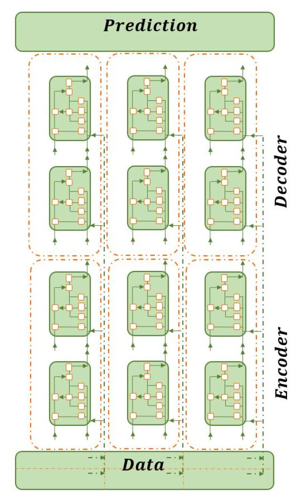
Figure 2: Ensemble of sequence-to-sequence networks

3.3 Resampling

Resampling is defined as constructing a number of samples from a dataset and refitting a specific model on each sample, hoping to perceive more accurate knowledge about the model. We use two methodologies, as follows:

• Additive resampling:
  To tackle the seasonality of the wind data, we divide the train and test datasets into a number of subsections equal to the EF. Then, we feed the whole train dataset plus a subsection of the train dataset into an independent network and evaluate a corresponding test subsection on that network. This division may result in discovering new functional relations within the subsection while they were hidden in the mixture. This method can be relatively expensive in terms of computations since each new epoch contains more samples. In the next subsection we discuss the fact that the DFO optimizes the EF number as one of its inputs. Hence, the number of the divisions for additive resampling depends on the dataset and the feature under study. We aim to reach the maximum potential of the parallel structure by using Additive resampling by optimizing the EF factor and directly using it in training and testing the networks.

• Bootstrap aggregating (bagging):
  We draw a number of samples with replacement and equal in size to the original dataset. For a large dataset, approximately $1-\dfrac{1}{e}$ fraction of any sample would be unique and the rest would be replicates [29]. Bagging is a well-known technique for statistical resampling [6].

A graphic explanation of the above techniques is shown in Figure LABEL:framework.

3.4 Scaled Trust Region Derivative-Free Optimization (SDFO-TR)

We modify a trust region version of DFO (DFO-TR). Compared to Bayesian optimization, DFOs are known to be time efficient and accurate, but the main deficiency is that in most studied DFO algorithms, the parameters are required to be purely continuous (their domain should be $\mathbb{R}$). Methods using DFO for integer variables basically boil down to enumeration or heuristics plus DFO for pure continuous variables. Here, we present scaled DFO-TR method capable of optimizing integer parameters. Algorithm 1 indicates in detail the scaled DFO-TR approach. This algorithm is based on [25, 5], with the following modifications:

Algorithm 1 SDFO-TR

1:Input: Budget $\mathcal{L},$ $z_{0}>0$, $0<\gamma_{1}<1<\gamma_{2}$, $0<\eta_{0}<\eta_{1}<1$, $\theta>1$, penalty coefficient $b$, upper bound on the function value $c$ and $[l^{i},u^{i}]\ i=1,2,...,P$.

2:Initialize $x_{0}=(x_{0}^{1},...,x_{0}^{P})$ where $x^{i}_{0}\in[l^{i},u^{i}]\ \forall i=1,2,...,P$.

3:Determine set of interpolation points $X\subseteq\mathcal{B}(x_{0},z_{0})$ to construct the model and evaluate $f(x),\forall x\in X$.

4:$x_{0}\leftarrow\text{argmin}_{x\in X}f(x)$.

5:for $k=0,1,2,...,\mathcal{L}$  do

6:     if $x_{k}^{i}\in[l^{i},u^{i}]$ $\ \forall i=1,2,...,P$ then

7:         Discard all points $x\in X$ where $\|x-x_{k}\|\geq\theta z_{k}$.

8:         $M_{k}(x_{k})\leftarrow f_{k}+g_{k}^{T}(x-x_{k})+\dfrac{1}{2}(x-x_{k})^{T}H_{k}(x-x_{k})$.

9:         $\bar{x}_{k}=\text{argmin}_{x\in\mathcal{B}(x_{k},z_{k})}M_{k}(x)$.

10:         $\rho_{k}=\dfrac{f(x_{k})-f(\bar{x}_{k})}{M_{k}(x_{k})-M_{k}(\bar{x}_{k})}$.

11:         if $|X|<\dfrac{(P+1)(P+2)}{2}$ then

12:              Append $\bar{x}_{k}$ to the set of interpolation points $X$.

13:         else if  $\big{(}\rho_{k}\geq\eta_{0}$ or $\|x-x_{k}\|<\max_{x\in X}\|x-x_{k}\|\big{)}$ then

14:              Substitute the point $\max_{x\in X}\|x-x_{k}\|$ with $\bar{x}_{k}$ in the set $X$.

15:         end if

16:         if $\rho_{k}\geq\eta_{1}$ then

17:              $x_{k+1}\leftarrow\bar{x}_{k}$ and $z_{k}\leftarrow\gamma_{2}z_{k}$.

18:         else if  $\rho_{k}<\eta_{0}$ then

19:              $x_{k+1}\leftarrow x_{k}$

20:              if $|X|>(P+1)$ then

21:                  $z_{k+1}\leftarrow\gamma_{1}z_{k}$

22:              else

23:                  $z_{k+1}\leftarrow{z_{k}}$

24:              end if

25:         else if  $\eta_{0}\leq\rho_{k}<\eta_{1}$ then

26:              $x_{k+1}\leftarrow\bar{x}_{k}$

27:              $z_{k+1}\leftarrow{z_{k}}$

28:         end if

29:         return $M_{k}(x_{k})$

30:     else

31:         return $c+b\sum_{i\in I^{*}}\min\{|x^{i}-l^{i}|,|x^{i}-u^{i}|\}$ where set $I^{*}$ contains indices for which $x^{i}\notin[l^{i},u^{i}]$

32:     end if

33:end for

1) The model is designed to minimize a black-box function in which the variables are within specified intervals instead of taking the whole $\mathbb{R}$ space. To achieve this, we further assume that the black-box loss function has an upper bound. Then for any parameter violating its interval, we consider the upper bound plus a penalty cost linearly related to the violation distance as the ultimate value of the function. This value would be considerably larger than the function value when all variables are inside their feasible regions. Therefore, the model has a logical incentive for not going out of the parameters’ feasible intervals. The observations are completely in support of this technique. At the beginning, the model explores through the parameters’ space randomly, and after some initial iterations, it mainly remains within their acceptable intervals. The mean arctangent absolute percentage error (MAAPE) has the known upper bound of $\dfrac{\pi}{2}$ (see 4.1). So, we mainly use this as the DFO loss function.

2) We further scale the intervals to $[0,1]$. Theoretically, scaling is not required because the trust region radius would handle different magnitudes for different parameters. However, scaling assists DFO in maintaining a good margin within acceptable intervals.

3) We bring the complexity of dealing with integer variables into the objective value. We divide the $[0,1]$ intervals into sub-intervals for which the objective value would remain unchanged. To fully grasp the idea, let’s assume that the proposed DFO optimizes a sequence-to-sequence ensemble considering the EF as its only input, and let’s further assume that EF $\in\{1,2,4,6\}$. We use MAAPE as the DFO loss function. Then, we can say algorithm 1 minimizes the following piecewise black-box function:

$$\text{DFO}(x_{ef})=\begin{cases}\dfrac{\pi}{2}-2x_{ef}&x_{ef}<0\\ S(x_{ef}=1)&0\leq x_{ef}<0.25\\ S(x_{ef}=2)&0.25\leq x_{ef}<0.5\\ S(x_{ef}=4)&0.5\leq x_{ef}<0.75\\ S(x_{ef}=6)&0.75\leq x_{ef}<1\\ \dfrac{\pi}{2}+2(x_{ef}-1)&x_{ef}>1,\\ \end{cases}$$

where $x_{ef}\in\mathbb{R}$ represents EF as the input variable, and $S(x_{ef}=i$) is the objective value of the parallel structure when we have $i$ independent sequence-to-sequence networks, $i\in\{1,2,4,6\}$. We considered the penalty coefficient $b=2$. Based on the scaling techniques we used in algorithm 1, we call this method SDFO-TR.

As shown in lines 1-4 of Algorithm 1, it starts to build an interpolation set based on some early function evaluations. Therefore, the initial value $x_{0}=(x_{0}^{1},...,x_{0}^{P})$ plays an important role, and having an acceptable guess may increase the performance [30]. There exist three major blocks inside the for loop:

• First block (lines 6-10): The algorithm constructs a quadratic approximation model $M_{k}(x)$ with current set of points and then determines its minimizer over the open ball $\mathcal{B}(x_{k},z_{k})$ where $z_{k}$ is the trust region radius. The success factor

  $$\rho_{k}=\dfrac{f(x_{k})-f(\bar{x}_{k})}{M_{k}(x_{k})-M_{k}(\bar{x}_{k})}$$ (1)

  is the measure of how well the model $M_{k}(x)$ mimics the actual black-box function.

• Second block (lines 11-15): The algorithm updates its set of interpolation points $X$ while keeping it poised. A quadratic polynomial $M(x)$ is an interpolation of a function $f(x)$ with respect to the set $X=\{x_{j}|j=1,...,m\}$ if

  $$M(x_{j})=f(x_{j}),\ \forall j=1,...,m.$$ (2)

  The set $X$ must remain poised with respect to the linear space of polynomials building $M(x_{j})$. We refer the reader to [5, 31] for details on poisedness of $X$.

• Third block (lines 16-29): The Trust Region (TR) update concept is borrowed. If the success factor $\rho>\eta_{1}$ which means it is close to one, then the algorithm both accepts the step and increases the radius to $\gamma_{2}z_{k}$, in order to explore the black-box function space more aggressively. If $\eta_{0}\leq\rho<\eta_{1}$, the algorithm still accepts the step but the radius remains the same. Finally, if $\rho_{k}<\eta_{0}$, then the algorithm rejects the step. The TR radius would stay the same if the quadratic approximation is based on at most $P$ evaluations, but if the approximation is based on more evaluations, it means the black-box objective function, fluctuates considerably over this particular region and the radius should be decreased.

In the instance we mentioned earlier, we solely examined the effects of one parameter to illustrate the SDFO-TR method. In general, any integer parameter with $t$ different feasible value, results in $t+2$ sections in the DFO objective function independently. We are dealing with training epochs, mini-batch sample size, LSTM hidden size, recurrent time step, optimization learning rate, number of stacked recurrent layers and EF hyperparameters in this proposal, and all of them receive integer values. Therefore, the DFO objective function initially contains millions of sections for above hyperparameter tuning. One may argue that by increasing the integer variables, the method could soon be intractable. To answer this, we know there can be several trends inside the feasible region for a parameter; for instance, like many other studies [32], increasing the mini-batch sample size after a limit would not help the network performance. There are studies showing that DFO may escape flat local minima and clear basins [25, 33]. Therefore, DFO avoids those points and many of the sections related to them. This is why we introduced the complexity into the function at the first place and let the DFO decides.

4 Experiments

In this section we evaluate the performance of the model for several tasks. First, we focus on the pure forecasting of wind speed, direction and power based on historical data of the same feature. Second, we aim to analyze the effects of wind speed on the actual output power produced by turbines.

4.1 Measures of Difference

Considering $b_{1},\dots,b_{n}$ and $\hat{b}_{1},\dots,\hat{b}_{n}$ as real and predicted measurements respectively, we mainly use the following measurement errors:

NRMSE:

$$\text{nrmse}=\dfrac{100\sqrt{\dfrac{1}{n}\sum_{i=1}^{n}(b_{i}-\hat{b}_{i})}}{R}$$ (3)

where $R$ is the range of the real measurements. Root Mean Squared Error (RMSE) is one of the most frequent measurement errors, but because it is scale dependent and we use this measure for different datasets, it is more logical to use its normalized version.

MAE:

$$\text{MAE}=\dfrac{\sum_{i=1}^{n}|b_{i}-\hat{b}_{i}|}{n}$$ (4)

Mean Absolute Error accounts for the average absolute difference between prediction and measurements.

MAAPE:

Mean Absolute Percentage Error (MAPE) expresses measurement absolute accuracy as a percentage. Mean Arctangent Absolute Percentage Error (MAAPE) intrinsically maintains the MAPE scale independency and intuitive interpretability while alleviating the drawback of dividing by zero.

$$\frac{1}{n}\sum_{i=1}^{n}\text{arct}\left(\left|\dfrac{b_{i}-\hat{b}_{i}}{b_{i}}\right|\right).$$ (5)

4.2 Alternative Algorithms

In this subsection, we summarize the other approaches in the literature which we compare the proposed algorithm with.
Seasonal auto regressive integrated moving average (SARIMA): Auto regressive moving average models [34, 35, 36] decompose the series into moving average and auto regressive ones. “Integrated” means the model uses a differencing process to reach stationarity considering a specific confidence level. A time series expresses seasonality when its expected value changes in a recurring manner. Seasonal ARIMA accounts for cases when the data exhibits seasonality. SARIMA models can be written as ARIMA$(p,d,q)(P,D,Q)_{m}$ where $p$ and $P$ are the time lags in the auto-regression for the trend and seasonal part, $d$ and $D$ refer to the differencing degree for trend and seasonal part, $q$ and $Q$ indicate the moving average order for both, and $m$ specifies how many periods are in each season. For time series $x_{0},x_{1},\cdots,x_{T}$, we define lag operator $L$ as: $L(x_{t})=x_{t-1},t=1,\cdots,T$. Then, one may implicitly express Seasonal ARIMA$(p,d,q)(P,D,Q)_{m}$ in a general form as follows:

$$(1-\sum_{i=1}^{p}\phi_{i}L^{i})(1-\sum_{i=1}^{p}\Phi_{i}L^{mi})(1-L)^{d}(1-L^{m})^{d}x_{t}=(1+\sum_{i=1}^{q}\theta_{i}L^{i})(1+\sum_{i=1}^{q}\Theta_{i}L^{mi})\epsilon_{t}$$

where $\epsilon_{t},\forall t=0,1,\cdots,T$ are zero-mean white noises, $\phi_{i}$ and $\Phi_{i},\forall i=1,2,\cdots,p$, are trend and seasonal auto-regression coefficients, respectively; and $\theta_{i}$ and $\Theta_{i},\forall i=1,2,\cdots,q$, are trend and seasonal moving average coefficients, respectively. It is clear that satisfactory performance of seasonal ARIMA depends on how accurately we choose its parameters. We compare our proposed method with SARIMA only for the online settings.

Extreme Learning Machine (ELM): ELM approaches [37, 38, 39] aim to generalize the learning procedure of feed-forward neural networks by randomly assigning parameters of hidden layer neurons. Input-hidden or hidden-hidden weights may remain unchanged through the learning process or simply accept their parents’ values in multi-layered ELM. This sharply distinguishes ELM from networks trained based on backpropagation. In addition, unlike the recursive weight updating approach used in backpropagation, one can update the input-hidden or hidden-hidden neuron weights at once in ELM, which results in several orders of magnitude faster performance time [40]. Here, we mainly focus on classic ELM and its improvement called fully online sequential-extreme learning machine [41, 42] (FOSELM) for the online setting comparisons.

Support Vector Regression: Unlike typical regression, which tries to minimize a least squared error, SVR seeks to construct a hyperplane for which the marginal error is minimized [43]. SVR utilizes functional relations called kernels to map interconnected input data into a higher dimension where the data is (almost) linearly separable. In SVR we have an $\epsilon$ margin of tolerance. In other words, two boundary hyperplanes exist at $\epsilon$ distance of the target hyperplane to contain most of the points, and the outliers are only allowed with a penalty cost added to the objective function. The penalty term can be looked at as a regularizer which assists the model to provide more general solutions and prevents overfitting and the most common type of them is an L2-norm. The data points on the two marginal hyperplanes that are responsible for their construction are called the support vectors. We refer the reader to MLSVM [44], which leverages hierarchical learning SVM, and [45] a novel SVM case study for more details on support vectors. Here, with the help of LIBSVM Python package [46] we implement the $\epsilon$-SVR and $\nu$-SVR methods.

Random Forrest (RF): RF is a meta predictor algorithm which includes an ensemble of Classification and Regression Trees (CART)[47]. CARTs are known to be easily interpretable, and each layer of their models contain Boolean logic. On the other hand, CARTs suffer from a generalization point of view. Because of their binary boundaries, they can easily overfit the train set. RF models improve the generalization performance of CARTs to a great extent. RF utilizes the bootstrap aggregating concept to focus on different parts of the dataset for every decision tree and then uses averaging techniques for prediction similar to our introduced method.

4.3 Wind Renewable Energy

As an alternative, wind energy offers a secure, competitive and sustainable option, releasing almost no greenhouse gases as well as consuming no water during its production. Dense wind farms across the globe are generating considerable amounts of electric power. The inherently time-varying nature of wind energy necessitates the development of a systematic framework to construct and forecast future wind characteristics [48]. Such a framework greatly enhances the flexibility of power systems to cope with irregular wind power patterns integrated in their portfolios. Therefore in the following sections, we investigate the performance of the proposed method for several tasks related to wind datasets.

4.3.1 Forecasting

In this part, we focus on very short- to long-term forecasting into the future considering high-resolution wind datasets. To this end, first we use an open-source national renewable energy laboratory (NREL) dataset for wind speed and wind direction forecasting . Table 2 indicates the details of the measurement station which this data is obtained. The time period between two consecutive measurements is 5 minutes. We consider only the first ten days of 2010 (or exactly $12\times 24\times 10=2880$ data points). We divide the data into 60 percent training, 20 percent validation and 20 percent testing for all methods. The design of the structure is conducted through training and then tested through validation to explore the best parameters’ results. None of the methods see the test set, and further, we have not touched the real dataset measurements in any way such as interpolation or normalization.

Table 2: National Renewable Energy Laboratory Station

Latitude	$39\mathrm{°}⁤54\mathrm{\prime }⁤38.34\mathrm{″}$ North;
Longitude	$105\mathrm{°}⁤14\mathrm{\prime }⁤5.28\mathrm{″}$ West
Sampling period	5 minutes
Elevation	1855 m

Table 3 demonstrates the results for several wind speed forecasting horizons. In the proposed method columns, we put those Ensemble Factors corresponding to the best performance in the parentheses. One can observe:

• SVR and ensemble structure achieve more valid and precise errors compared to the other two methods.

• Additive resampling works marginally better than bagging one.

• The proposed method performs superior with the increasing of the forecasting horizon. In other words, some of the alternatives such as SVR reach smaller errors for one- or six-step-ahead estimations, but for medium- to long-term forecasting, we observe satisfactory improvement by sequence networks, particularly considering A-Sampling. We argue this can be due to the structure of the proposed method, which can discover hidden relations in deeper forecasting horizons.

• Huge jumps occur in the error values by going from forecasting one step into the future to six steps. But this is not the case for deeper horizons. We even observe that some methods reach better errors for 48 steps compared to 36 steps, or 72 steps compared to 48 steps.

Table 3: MAAPE, NRMSE and MAE comparison for wind speed

MAAPE
			ELM		SVR			RF		Proposed Method
	Time Steps				$\epsilon$-SVR	$\nu$-SVR				A-Sampling (EF)	B-Sampling (EF)
	1		0.153		0.151	0.151		0.179		0.149 (6)	0.154 (4)
	6		0.335		0.325	0.326		0.342		0.316 (2)	0.320 (2)
	12		0.415		0.401	0.402		0.417		0.380 (1)	0.397 (1)
	24		0.478		0.447	0.447		0.499		0.430 (1)	0.447 (1)
	36		0.503		0.465	0.466		0.512		0.448 (4)	0.477 (2)
	48		0.500		0.461	0.459		0.493		0.435 (1)	0.468 (1)
	72		0.519		0.459	0.459		0.517		0.446 (1)	0.487 (1)
NRMSE
			ELM		SVR			RF		Proposed Method
	Time Steps				$\epsilon$-SVR	$\nu$-SVR				A-Sampling	B-Sampling
	1		7.520		5.895	5.896		6.925		5.966	5.910
	6		15.867		14.442	14.4284		16.328		14.392	14.203
	12		20.146		17.761	17.7404		19.780		18.678	17.942
	24		23.894		19.596	19.715		24.109		18.882	20.599
	36		22.930		21.041	21.103		25.988		20.641	21.731
	48		22.809		19.660	19.620		24.180		18.284	20.474
	72		22.704		17.629	17.534		23.160		17.123	18.787
MAE
			ELM		SVR			RF		Proposed Method
	Time Steps				$\epsilon$-SVR	$\nu$-SVR				A-Sampling	B-Sampling
	1		0.444		0.370	0.369		0.449		0.372	0.373
	6		0.989		0.944	0.945		1.074		0.952	0.937
	12		1.293		1.210	1.210		1.331		1.235	1.217
	24		1.539		1.370	1.380		1.653		1.298	1.417
	36		1.618		1.448	1.452		1.727		1.398	1.497
	48		1.550		1.357	1.351		1.601		1.242	1.409
	72		1.548		1.227	1.218		1.544		1.151	1.305

Table 4 indicates the results for similar forecasting horizons for wind direction on the same subsample of the NREL dataset we used before. One can observe:

• RF, SVR, and ensemble structure share most of the best results among themselves. There is no clearly superior method.

• Bagging resampling performs slightly better than additive for short-term wind direction forecasting while for long-term ones, the reverse is true.

• For long-term forecasting, the ensemble structure mostly performs better than the alternatives. For instance, A-Sampling reaches $0.287$ MAAPE while ELM, as the best alternative, reaches $0.402$.

Table 4: MAAPE, NRMSE and MAE comparison for wind direction

MAAPE
			ELM		SVR			RF		Proposed Method
	Time Steps				$\epsilon$-SVR	$\nu$-SVR				A-Sampling (EF)	B-Sampling (EF)
	1		0.331		0.071	0.087		0.096		0.125 (1)	0.079 (6)
	6		0.341		0.148	0.165		0.186		0.164 (1)	0.159 (6)
	12		0.357		0.401	0.214		0.235		0.209 (1)	0.208 (2)
	24		0.369		0.447	0.267		0.281		0.300 (1)	0.291 (2)
	36		0.382		0.465	0.333		0.353		0.329 (2)	0.336 (2)
	48		0.384		0.461	0.389		0.430		0.326 (2)	0.339 (6)
	72		0.402		0.459	0.457		0.453		0.287 (2)	0.326 (1)
NRMSE
			ELM		SVR			RF		Proposed Method
	Time Steps				$\epsilon$-SVR	$\nu$-SVR				A-Sampling	B-Sampling
	1		20.407		7.252	7.928		8.752		11.653	7.772
	6		21.669		14.554	15.797		15.194		14.884	14.430
	12		22.141		19.369	21.382		18.730		18.228	17.911
	24		23.603		22.009	23.958		23.902		21.486	20.963
	36		43.000		24.412	27.882		26.365		29.516	28.198
	48		23.073		27.570	31.508		25.503		28.820	29.223
	72		92.813		28.714	28.061		25.904		30.861	28.464
MAE
			ELM		SVR			RF		Proposed Method
	Time Steps				$\epsilon$-SVR	$\nu$-SVR				A-Sampling	B-Sampling
	1		62.555		11.842	15.265		16.343		27.414	13.457
	6		64.623		27.597	32.112		34.049		32.926	29.093
	12		68.037		39.502	47.211		46.758		41.046	40.378
	24		71.275		50.738	55.979		65.802		55.057	54.217
	36		78.023		62.537	71.256		73.336		78.593	79.029
	48		72.834		74.934	86.684		72.169		76.020	80.233
	72		90.937		85.218	80.023		75.403		70.961	76.431

One of the fundamental features of wind energy is the actual output power of the wind absorbed by the turbines. To investigate the performance of the methods for forecasting this feature, we use the same open-source dataset of GECAD that we used to conduct the seasonality experiment but this time we consider the first ten days of 2011 (or exactly $6\times 24\times 10=1440$ data points). Table 5 reports the power estimation results. One can observe:

• The proposed method, considering both resampling techniques, clearly has an advantage over the others. Like previous tables, the deeper the prediction horizon is, greater the margin becomes.

• Most of the reported errors for 48 and 72 steps into the future are pretty close to the ones with shallower horizons. This may be due to the fact that all three error measurements have the sense of normalization inside them, which makes them comparable in separate contents, but we argue that it can be due to the repetitive patterns of the wind energy as well.

• The bootstrap aggregation technique performs best in short to medium horizons, while additive techniques have the best performance for long-term predictions. This was the case in the wind direction estimation, as well, with less intensity.

Table 5: MAAPE, NRMSE and MAE comparison for wind power on GECAD data

MAAPE
			ELM		SVR			RF		Proposed Method
	Time Steps				$\epsilon$-SVR	$\nu$-SVR				A-Sampling (EF)	B-Sampling (EF)
	1		0.580		0.324	0.344		0.357		0.390 (1)	0.396 (2)
	6		0.659		0.518	0.512		0.568		0.461 (2)	0.453 (1)
	12		0.638		0.585	0.583		0.611		0.465 (1)	0.459 (1)
	24		0.625		0.616	0.621		0.613		0.428 (2)	0.463 (1)
	36		0.677		0.644	0.626		0.670		0.411 (2)	0.459 (2)
	48		0.641		0.616	0.583		0.631		0.397 (2)	0.396 (1)
	72		0.649		0.668	0.667		0.617		0.402 (2)	0.400 (2)
NRMSE
			ELM		SVR			RF		Proposed Method
	Time Steps				$\epsilon$-SVR	$\nu$-SVR				A-Sampling	B-Sampling
	1		23.619		10.866	11.043		12.197		19.820	21.730
	6		28.484		19.509	19.287		23.237		24.231	23.470
	12		29.429		23.788	23.420		26.708		24.915	24.905
	24		29.163		26.632	26.529		28.258		25.350	25.699
	36		185.49		27.019	26.012		32.086		24.871	24.955
	48		33.912		24.697	23.542		27.280		23.206	23.157
	72		31.984		26.971	26.698		27.525		23.443	23.434
MAE
			ELM		SVR			RF		Proposed Method
	Time Steps				$\epsilon$-SVR	$\nu$-SVR				A-Sampling	B-Sampling
	1		74.781		32.873	33.821		36.987		54.072	58.323
	6		97.460		64.508	63.654		76.970		69.800	67.899
	12		98.999		81.504	803.29		90.102		72.363	71.928
	24		96.353		92.036	92.307		94.770		73.867	74.637
	36		167.68		93.295	89.458		107.01		70.198	70.379
	48		97.394		83.126	77.641		90.284		64.730	64.619
	72		99.125		92.365	91.649		88.576		64.921	64.900

Furthermore, by considering all three tables together:

• Wind power prediction is the most challenging one and requires more diligence. Some of the methods’ errors eventually become pretty enormous for power forecasting. Wind direction prediction stands second.

• MAAPE can be seen as a true unitless method across the separate tables. In addition, its value changes with viscosity and this makes its overall interpretation easier.

• The Extreme Learning machine performs worse compared to the other methods. Random forest is less consistent and experiences more fluctuations. It reaches the best performance in cases such as those of the NRMSE errors for wind direction, but performs the worst for wind speed regarding the same error measurement.

• SVR performs solid for short-term predictions but its performance fades away when considering deeper horizons.

• We suggest bagging resampling for short horizons and additive sampling for longer terms.

Finally, we investigate the importance of the wind speed for forecasting the wind output power. In other words, we aim to explore the important question of how much the output power of wind renewable energy is based on historical data on the wind speed at that location. Hence, we only use wind power as the labels and not the input to the model. We still use the same dataset as the one for power prediction. Table 6 indicates the comparisons. We can observe:

• The errors of forecasting the wind output power based on wind speed are very close to the ones based on power historical data. This confirms the strong correlation between the two. The errors are even smaller for short horizons. Therefore, we suggest using wind speed to estimate accurate wind power along with historical power data.

• ELM provides satisfactory performance for short-term cases, but it fails to maintain its superiority.

• RF and our proposed methods accomplish the best performance specifically when the horizon increases.

Table 6: MAAPE, NRMSE and MAE comparison for wind power based on wind speed on GECAD data

MAAPE
			ELM		SVR			RF		Proposed Method
	Time Steps				$\epsilon$-SVR	$\nu$-SVR				A-Sampling (EF)	B-Sampling (EF)
	1		0.276		0.332	0.325		0.369		0.384 (1)	0.387 (1)
	6		0.569		0.511	0.516		0.553		0.488 (1)	0.471 (1)
	12		0.570		0.569	0.577		0.604		0.468 (1)	0.468 (4)
	24		0.624		0.617	0.617		0.603		0.443 (2)	0.463 (6)
	36		0.634		0.631	0.628		0.658		0.402 (2)	0.459 (2)
	48		0.589		0.592	0.585		0.610		0.381 (2)	0.454 (1)
	72		0.635		0.674	0.659		0.630		0.398 (2)	0.458 (2)
NRMSE
			ELM		SVR			RF		Proposed Method
	Time Steps				$\epsilon$-SVR	$\nu$-SVR				A-Sampling	B-Sampling
	1		8.730		10.778	10.761		12.248		16.285	20.219
	6		21.639		19.341	19.429		22.293		25.231	22.870
	12		23.838		22.797	23.185		25.166		25.140	25.116
	24		27.409		26.547	26.312		28.092		26.474	25.708
	36		28.656		26.393	26.237		30.687		25.621	24.885
	48		24.959		23.716	23.472		26.683		23.916	23.156
	72		26.263		27.262	26.331		26.865		25.743	23.449
MAE
			ELM		SVR			RF		Proposed Method
	Time Steps				$\epsilon$-SVR	$\nu$-SVR				A-Sampling	B-Sampling
	1		26.959		32.803	32.500		38.394		46.896	54.200
	6		74.355		63.622	64.163		73.477		73.863	67.364
	12		79.267		77.863	79.386		86.233		73.045	72.989
	24		93.151		91.947	91.365		93.178		77.506	74.657
	36		94.274		90.645	90.001		102.60		71.839	70.230
	48		81.849		78.804	77.739		86.790		65.302	64.615
	72		88.215		93.654	90.036		88.677		69.010	64.935

4.3.2 Feature Selection

In this section we aim to tackle the concept of feature selection. We develop a framework to select the important inputs affecting wind power and throw away unsatisfying ones. We bring SDFO-TR one more time into the design of the framework, and not only for tuning. For each feature, we introduce a variable and we let SDFO-TR decide whether to use the feature’s data. This injects all the complexity into the DFO optimization. Therefore, the DFO performance can be affected when it encounters a large number of features. However, the process benefits from clear interpretation. In other words, SDFO-TR ideally identifies the exact list of dominant features. It is worth mentioning that the whole feature selection process is automated. In the algorithm 1, we increase the number of variables as $x=(x^{1},...,x^{(P+Q)}),$ where $Q$ is the total number of features and $x^{i}\in\left[0,1\right],\ \forall i=P+1,...,P+Q,$ with $\dfrac{1}{2}$ being considered as the threshold for whether to choose the feature. Figure LABEL:framework illustrates the proposed method in a general view. The SDFO-TR algorithm chooses the features and parameters for the ensemble structure up to the budget $\mathcal{L}$.

We want to investigate the effect of different environmental characteristics on wind speed and therefore indirectly on wind power. This is not a prediction since we do not use wind speed historical data as an input to the process, but only as the labels to evaluate the errors. That is, we are certain about the fact that historical data on wind speed can greatly enhance its prediction, and Table 3 is in fact dedicated to this. However, to correctly investigate other major factors, we cast aside wind speed from the inputs and only use it as the output label for accuracy evaluations.

To this end, we focus on another open-source GECAD dataset , which is rich in the number of presented features. The features are [Temperature (C), Dew-point (C), Pressure (Pa), Wind Direction, Wind Direction Degrees ($\degree$), Wind Speed (KMH), Wind Gust (KMH), Humidity, Hourly Precipitation (MM), daily rain (MM), Solar Radiation (Watt/$m^{2}$)]. We always choose Wind Direction Degrees column so that we have at least one feature. We further omit the column Wind Direction because it is a duplicate of Wind Direction Degrees column but expressed qualitatively. We focus on the first ten days of the dataset due to computational limitations and the further train/test division routines are as same as previous experiments. All the models have access to up-to-date measurements at each time step except wind speed which is under study. To the best of the authors’ knowledge, this comparison to find the most effective elements on wind speed has not been studied.

Table 7 represents the effect of using SDFO-TR for feature selection as well as a comparison with Spearmint Bayesian optimization hyperparameter tuning method. We compare the presented method with and without feature selection for both of the resampling techniques. The Spearmint is designed to tune parameters of one sequence-to-sequence network. We tune all the parameters considered in the proposed method with Spearmint except the EF. We internationally focus on one sequence-to-sequence network to see the impact of EF on the performance of the proposed structure. In other words, the results showing in Table 7, indicate the differences between DFO and Spearmint hyperparameter methods combined with the effect of using ensemble of sequence-to-sequence networks versus single network.

Throughout the paper, we report three different error metrics. One can consider any of these metrics as the loss function of DFO or Spearmint. So far in all the studies, we considered MAAPE as the main objective function of DFO and then we obtain the predictions. After we obtained the predictions and the optimization process is done, we calculate the other two errors based on the predictions for report purposes. The three errors are mostly in a harmony having DFO as the tuning method. However, We realize it is not the case for Spearmint method. In other words, we may optimize the process considering MAAPE and reach a satisfying MAAPE error but at the same time we obtain relatively large value for NRMSE or MAE. Having said this, we conduct three experiments with Spearmint for each of the three error metrics as its objective function.

From the information of Table 7 one can argue:

• Methods with the selected group of features have superior performance compared to those using all the information.

• For ensemble structure, additive resampling in general is more robust compare to bagging.

• Spearmint performance is promising when we consider MAE and MAAPE as its objective function but its performance is inferior compare to other methods when we use NRMSE as its objective function. Moreover, when we optimize Spearmint with MAAPE, it reaches the best accuracy between all the methods but simultaneously it reports not a satisfying NRMSE. We conclude that Spearmint exploits the tuning process with one objective function to such an extent that it can generally result in inferior values for other objectives.

• The most robust performance of Spearmint is when we optimize MAE as its objective. In this case, the results are in a close tie with the proposed structure with Additive resampling.

• Temperature, Dew-point, wind gust and solar radiation are mostly chosen by different methods which shows their important correlations with wind speed. It is natural to guess that wind gust contains information about wind speed. Please note that we always select wind wind direction degrees column.

• Pressure is mainly not chosen in the selected group by majority of the methods. Therefore, we suggest there is less correlation between wind speed and pressure.

Table 7: Feature selection for wind speed on GECAD data

Method		EF		MAAPE		NRMSE		MAE		Selected Features
Additive (all feature)		1		0.834		11.025		2.569		[1,1,1,1,1,1,1,1,1]
Bagging (all feature)		3		0.943		11.028		3.615		[1,1,1,1,1,1,1,1,1]
Additive (feature Selection)		5		0.826		11.013		2.490		[1,1,0,1,1,0,1,1,1]
Bagging (feature Selection)		2		0.924		9.751		3.199		[1,1,0,1,1,0,0,0,1]
Spearmint (Obj. function: MAAPE)		1		0.690		12.225		3.152		[1,1,0,1,1,0,0,0,1]
Spearmint (Obj. function: NRMSE)		1		0.805		17.337		4.778		[1,0,1,1,1,1,0,1,1]
Spearmint (Obj. function: MAE)		1		0.846		11.104		2.441		[0,1,0,1,1,1,0,0,0]

4.3.3 Online Forecasting

So far, all of the studies we have discussed are conducted in an offline setting which means we train the model on a train dataset and then test its performance on the test set. On the other hand, in online settings the model simultaneously learns through the dataset with information being revealed one step at a time. Here, we briefly address the online forecasting setting. Any online method estimates (mostly) one step ahead into the future, and then the realization of that forecast happens subsequently and the model has access to it. Afterwards, the model estimates the next point and the online process goes on. To this end, the division of the data into train, validation and test does not make sense. Instead, the model updates its learning during the process at each time step. In other words, the model learns from some initial data and then learns from and is evaluated by the rest of the data simultaneously. Having said this important difference, we still call the second part of the dataset as the test set, but note that the model learns through the test set as well.

In this setting, one can modify the two resampling techniques mentioned above, but we simplify our model to have only one sequence-to-sequence network. Therefore, there is no resampling used in this section. Once again we utilize the GECAD dataset exactly as we used it for the prediction of wind power output in Table 5. This time, the entire test set, or equivalently the last 20 percent of the whole dataset, is considered as the online setting test set. We do this so that we can compare the errors in regular forecasting with online case.

Table 8 reports the comparisons between the proposed method and the SARIMA and FOSELM methods that were discussed in Section 4.2. It is worth mentioning that for every single point in the online test set, we fit a whole new SARIMA model and estimate one step ahead into the future, and at the end, we evaluate the errors. We use a buffer of 100 points for each of these SARIMA models, and disregard the rest of the dataset because more than this buffer size only complicates the SARIMA structure and does not help with the performance. We found that FOSELM method very sensitive to the tuning of its parameters. Therefore, the reported results for this method are the best ones out of 10 independent runs. We can observe:

• The proposed Method outperforms the other two by a significant margin.

• The proposed Method results are better compared to the similar case in regular forecasting in Table 5. The reason is that in the online settings, we allow the model to learn during the testing period.

Table 8: Online Forecasting for wind power

Method		MAAPE		NRMSE		MAE
FOSELM		0.614		25.272		82.644
SARIMA		0.424		17.272		50.649
Proposed Method		0.280		10.878		31.597

Figure 3 demonstrates actual test set along with the online forecasting results of the three methods. We mention one more time that after each prediction, the models observe the ground truth values of that time step and they use it in the next prediction. We can see that SARIMA and our method have a clear advantage over FOSELM. In addition, both SARIMA and FOSELM estimate some negative values for the output power which indicate the considerable gap between the actual non-negative output power and the predictions from these two methods.

Figure 3: Wind power online forecasting. Inset boxes illustrate zoomed-in portions

4.4 Solar Renewable Energy Forecasting

Converted into electrical and thermal energy, solar renewable energy is one of the most promising alternatives for fossil fuels, originating from radiant light and heat from the Sun. In terms of global capacity, solar Photovoltaics (PV) is among the first three renewable sources besides Hydroelectricity and wind powers [49]. Here, we focus on prediction of global horizontal irradiance (GHI) which is the total amount of terrestrial radiation falling on a surface horizontal to the surface of the ground. GHI is of a certain importance for photovoltaic conversion processes because it is used for PV output power calculation and it accounts for both of the direct normal irradiance (DNI) and diffuse horizontal irradiance (DHI) [50]. To this end, we use an open source solar data provided by national solar radiation database (NSRDB) [51] for central park New York located at $(40.77,-73.98)$ coordination for year 2017 . The dataset contains measurements thirty minutes apart each. The raw dataset roughly contains 50 percent zero GHI which accounts for the hours where the exact location does not receive any radiant light from the Sun. We first conduct some forecastings on the raw dataset without omitting any zeros. Then, we eliminated all the zeros and conduct the same experiment. Comparisons confirm that eliminating the zeros significantly improves the accuracy of the prediction. We consider the first 4320 data points (three first months of 2017). Considering MAAPE as the error metric, Table 9 indicates the comparison between the case where we considered all the measurements fore forecasting versus the case where we eliminated the zeros. The datasets for the two experiences are not exactly the same but MAAPE as previously mentioned in Section 5 is the most robust error metric among the metrics we studied and it is reliable for relative comparisons. As one can see in Table 9, the MAAPE errors reported for the reduced dataset are noticeably less than the raw dataset. Therefore, for the comprehensive comparisons with alternative methods in the following table, we focus on the reduced dataset.

Table 9: MAAPE error comparison between GHI Raw and reduced datasets.

		Additive Resampling				Bootstrap Resampling
		MAAPE Error				MAAPE Error
Time Steps		Raw Dataset		Reduced Dataset		Raw Dataset		Reduced Dataset
1		1.020		0.425		1.112		0.500
6		1.025		0.605		1.167		0.624
12		1.114		0.627		1.192		0.621
24		1.174		0.615		1.206		0.624
36		1.158		0.620		1.194		0.626
48		1.121		0.594		1.190		0.624
72		1.209		0.623		1.216		0.623

We explore GHI estimation and compare the results of the proposed method with SVR and RF. Table 10 reports the findings. As shown previously, the proposed method considering both resampling techniques is more robust against increasing the forecasting horizon. SVR and RF methods have advantages over the method for the very short forecasting steps, but for longer forecasting horizons, the method performs relatively better. Moreover, the reported MAAPE error for GHI even on reduced dataset is higher than reported MAAPE error of wind direction and speed and is relatively close to errors mentioned for forecasting wind power. That is, the stochasticity of the GHI is considerably high.

Table 10: MAAPE, NRMSE and MAE comparison for global horizontal irradiance (GHI)

MAAPE
			SVR			RF		Proposed Method
	Time Steps		$\epsilon$-SVR	$\nu$-SVR				A-Sampling (EF)	B-Sampling (EF)
	1		0.358	0.359		0.345		0.425 (1)	0.500 (4)
	6		0.634	0.640		0.603		0.605 (1)	0.624 (1)
	12		0.676	0.724		0.687		0.627 (1)	0.621 (1)
	24		0.697	0.718		0.692		0.615 (3)	0.624 (1)
	36		0.739	0.743		0.728		0.620 (3)	0.626 (4)
	48		0.717	0.730		0.717		0.594 (6)	0.624 (4)
	72		0.726	0.768		0.736		0.623 (1)	0.623 (2)
NRMSE
			SVR			RF		Proposed Method
	Time Steps		$\epsilon$-SVR	$\nu$-SVR				A-Sampling	B-Sampling
	1		10.855	10.624		11.731		24.226	35.504
	6		27.105	26.500		23.963		34.576	39.674
	12		30.675	37.012		28.449		39.795	39.145
	24		35.442	38.247		31.311		40.790	40.122
	36		37.697	37.738		34.518		40.976	40.312
	48		37.245	36.398		35.113		38.064	39.961
	72		34.407	36.813		37.015		39.221	39.157
MAE
			SVR			RF		Proposed Method
	Time Steps		$\epsilon$-SVR	$\nu$-SVR				A-Sampling	B-Sampling
	1		66.248	63.7105		74.513		145.236	213.343
	6		191.277	188.178		169.543		222.690	249.781
	12		215.607	255.722		207.938		251.782	247.761
	24		242.326	261.320		224.981		259.683	253.450
	36		269.622	270.761		247.277		256.896	253.009
	48		254.923	255.712		246.723		229.296	249.469
	72		240.599	263.872		255.920		240.421	240.045

4.5 Feature Selection in Wave Renewable Energy

As long as wind blows with sufficient stability to provide continuous ocean waves, marine power contains promising potential as alternative energy [52]. The marine infrastructure for harnessing such a power, however, is less developed compare to wind and solar sources at the time [53]. One of the main reasons is that there are few studies investigating major contributors to ocean wave output power. Therefore, in this section we aim to find the most important marine features affecting the wave output power. We use the case study established by [3] in the east coast of the U.S. The case study explores the effect of different ocean features, recorded by several sensors of different distances, on the significant wave height and ocean power of specified location. They use an Elastic net (EN) regularizer for feature selection. Similar to the study, we consider 53 features of 5 different nearby buoys. For more details on the buoys and their selected features, please see the Appendix B. As far as the authors’ knowledge extend, this study is the first study to utilize DFO as a designer in the concept of ocean wave energy.

To demonstrate a fair comparison of DFO method with other tuning/feature selection methods, we consider the exact ensemble structure of the networks as well as the exact marine features for a case where Spearmint is responsible for all the designing and tuning tasks. First, we consider 53 binary variables indicate whether we use any combination of the features. Second, we reserve an integer variable for EF and finally, we take into consideration the structural features of the sequence-to-sequence network such as number of stacked LSTM layers, learning rate and etc. The total number of features ends up to be 62 for both DFO and Spearmint. The data size is 3422 points. Therefore, the feature selection is conducted on a dataset of $3422\times 62$. We refer the reader to Appendix B, to see the selected group of marine features for both DFO and Spearmint techniques. Table 11 indicates the results of the comparison. First two rows are reported from [3]. Furthermore, to be consistent with the mentioned study we used RMSE and HUBER losses besides MAAPE. In addition, we limit the experiments to additive resampling for DFO and Spearmint.

Table 11: Ocean wave power output.

		Wave Power Output
Technique		MAAPE		RMSE		HUBER
RF		0.56		3.43		5.62
Elastic Net		0.45		4.53		2.21
Spearmint		0.40		2.88		1.08
DFO		0.35		3.15		1.23

We observe:

• DFO and Spearmint reject using many features and this indicates the importance of feature selection for renewable energy concept. The most important features to foresee the ocean wave output power of an unknown location are its nearby air temperature, significant wave height and wind speed. (See Appendix B).

• The two ensemble methods (DFO and Spearmint) have considerable advantage over the other two methods. The results suggest using of the parallel structures.

• There are advantages and disadvantages comparing EN with DFO and Spearmint techniques. EN can partially utilize any input feature and in the cases where the datasets contain valuable information in many separate features, it can be helpful. DFO and Spearmint, however, accept or reject entire data related to a feature. Findings confirm that using the latter approach results in better accuracy. One can argue that stochasticity involved in the nature of the renewable sources can be one of the reasons that DFO and Spearmint omit many features.

• In contrast to wind speed feature selection study, DFO rejects using of many of the features. This can be a confirmation on the fact that ocean waves are irregular waves with few solid correlations between them and other marine features.

5 Conclusion

We introduce an ensemble of sequence-to-sequence neural networks and combine the structure with derivative-free optimization and other tuning/designing techniques such as Spearmint Bayesian optimization to tackle both the forecasting and feature selection of any multivariate time series including but not limited to renewable energy sources. We introduce additive resampling technique to take into account the repetitive patterns of the data and to further utilize the parallel structure to its maximum extent possible by assigning different parts of the training set to separate networks. In addition to additive resampling, the well-established bagging resampling is considered throughout the paper.

The findings confirm the parallel structure can be successfully integrated with other optimization techniques such as DFO and Spearmint. Moreover, results indicate the superiority of the proposed method compare to many established machine learning approaches in particular in cases where one targets deeper steps into the unknown future.

Then, we present three independent case studies about wind, solar and wave renewable energy sources. All three sources are among the most affordable and scalable renewable sources but their ever-changing nature requires a framework to foresee its future outcomes. To this end, we forecast wind speed, wind direction, wind power output, global horizontal irradiance along with ocean wave power output. We realize wind output power and global horizontal irradiance have marginally bigger measurement errors compare to wind speed and direction which means more irregularity in wind power and global irradiance. In addition, we explore the effect of wind speed on forecasting wind output power. Results suggest that wind speed is actually a reliable indicator for the possible wind output power in particular for short term forecasts. This confirms a solid correlation between wind speed of a location and the produced wind output power. Moreover, we study forecasting of global horizontal irradiance. We suggest reducing the GHI datasets into nonzero measurements for better performance.

Then, we aim to find the most effective environmental and marine features on wind speed and ocean wave output power respectively. To this end, we modify the framework to automatically select major features and discard those that are not useful to estimation of the under study feature. Studies show temperature, Dew-point, wind gust and solar radiation are four most important features affecting wind speed which are chosen by majority of the methods. Significant wave height, wind speed and air temperature are among the most principal marine features affecting ocean wave output power. Moreover, we investigate online forecasting concept. The results substantiate the superiority of the method for forecasting wind power compare to other methods.

Ensemble network designs are promising structures and we suggest investigation of those in other aspects of renewable energy systems. Furthermore, employing DFO as a decision maker for the design of a parallel structure can be explored in many other machine learning disciplines.

Appendix A LSTM and Sequence-to-Sequence Structures

We consider $[a_{1},a_{2},...,a_{T}]$ as an input sequence of an LSTM cell. For an LSTM cell for any time step $l=1,..,T$, we have [54]:

$$f_{l}=\text{sigm}\left(W_{fa}a_{l}+W_{fh}h_{l-1}\right)$$ (6)

$$p_{l}=\text{sigm}\left(W_{pa}a_{l}+W_{ph}h_{l-1}\right)$$ (7)

$$o_{l}=\text{sigm}\left(W_{oa}a_{l}+W_{oh}h_{l-1}\right)$$ (8)

$$c_{l}=f_{l}\odot c_{l-1}+p_{l}\odot\text{tanh}\left(W_{ca}a_{l}+W_{ch}h_{l-1}\right)$$ (9)

$$h_{l}=o_{l}\odot\text{tanh}(c_{l}),$$ (10)

where $\odot$ means element-wise matrix product, $a_{l}\in\mathbb{R}^{Q}$, $h_{l}\in\mathbb{R}^{H}$ are the input and hidden vectors, $f_{l}\in\mathbb{R}^{H}$, $p_{l}\in\mathbb{R}^{H}$, $o_{l}\in\mathbb{R}^{H}$, $c_{l}\in\mathbb{R}^{H}$ are forget, input, output and cell gates respectively, and at last $Q$ and $H$ are the input feature and LSTM hidden sizes. The actual output of each LSTM cell is its hidden layer.

A sequence-to-sequence network contains two separate recurrent structures which in our case are two LSTMs. First structure (encoder) reads the input sequence $[a_{1},a_{2},...,a_{T}]$ considering $h_{0}=c_{0}=0$ and gives $h_{T}$ vector as its output. Second structure (decoder) uses $h_{T}$ as its initial state and deliver the prediction $[b_{T+T^{\prime}}]$.

Appendix B Ocean Wave Case Study

Figure 4 schematically shows six active measurement stations of NOAA. Table 12 tabulates the necessary information of the measurement buoys. This experiment is designed to see the effect of other ocean features on possible output power at a different location. We aim to forecast the ocean output power at station 44008 with the features from the other 5 adjacent buoys as mentioned in Table 13. The abbreviations of the features are explained in Table 14.

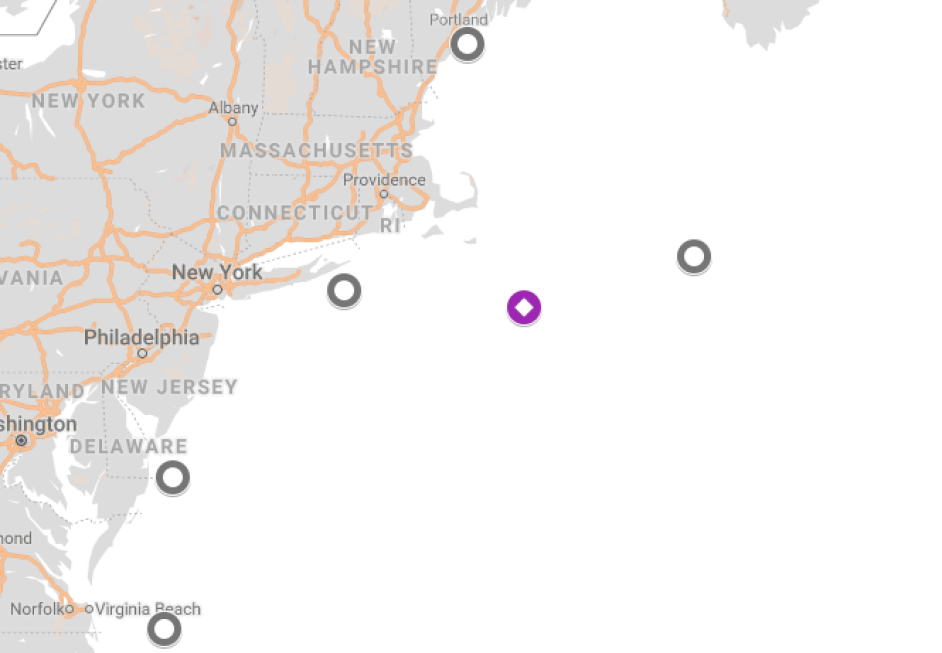
Figure 4: NOAA measurement stations for Ocean Wave power output Case study conducted by [3].

Table 12: NOAA measurement stations

Station ID number		44007	44008	44009	44013	44014	44017
Coordination		(70.14, 43.52)	(69.24, 40.50)	(74.70, 38.45)	(70.65, 42.34)	(74.84, 36.60)	(72.04, 40.69)
Depth of water		26.5	74.7	30	64	47	48

Table 13: 53 input features and output label

Features		Station 44007:		WDIR7	WSPD7	GST7	WVHT7	DPD7	APD7	MWD7	PRES7	ATMP7	WTMP7	DEWP7
		Station 44009:		WDIR9	WSPD9	GST9	WVHT9	DPD9	APD9	MWD9	PRES9	ATMP9	WTMP9
		Station 44013:		WDIR13	WSPD13	GST13	WVHT13	DPD13	APD13	MWD13	PRES13	ATMP13	WTMP13
		Station 44014:		WDIR14	WSPD14	GST14	WVHT14	DPD14	APD14	MWD14	PRES14	ATMP14	WTMP14	DEWP14
		Station 44017:		WDIR17	WSPD17	GST17	WVHT17	DPD17	APD17	MWD17	PRES17	ATMP17	WTMP17	DEWP17
Label		Station 44008:		Output power

Table 14: Ocean wave features description

Abbreviation		Description		Abbreviation		Description
WDIR		Wind direction		WSPD		Wind speed (m/s)
WVHT		Significant wave height (meters)		DPD		Dominant wave period (seconds)
MWD		Direction of DPD		PRES		Sea level pressure (hPa)
GST		GST Peak 5 or 8 second gust speed (m/s)		APD		Average wave period (seconds)
WTMP		Sea surface temperature (Celsius)		DEWP		Dewpoint temperature
ATMP		Air temperature (Celsius)

The selected group of marine features for DFO is [WVHT7, WVHT9, WSPD13, WVHT13, WVHT14, WVHT17] and the rest are not selected. The selected group of features for Spearmint is [WSPD7, WVHT7, APD7, PRES7, ATMP7, DEWP7, WSPD9, WVHT9, MWD9, PRES9, ATMP9, WDIR13, GST13, APD13, PRES13, ATMP13, WTMP13, WSPD14, WVHT14, DPD14, APD14, ATMP14, WDIR17, WSPD17, DPD17, ATMP17]. Therefore, air temperature, significant wave height and wind speed are the most gainful features to consider.

Acknowledgments

This research was partially supported by the National Science Foundation via the CyberSEES grant #1442858. The authors are accountable for the conclusions documented in the paper and the points claimed in the article have not been endorsed by the sponsoring agency.

References

- Zhou et al. [2011] Junyi Zhou, Jing Shi, and Gong Li. Fine tuning support vector machines for short-term wind speed forecasting. Energy Conversion and Management, 52(4):1990–1998, 2011.
- Li and Shi [2010] Gong Li and Jing Shi. On comparing three artificial neural networks for wind speed forecasting. Applied Energy, 87(7):2313–2320, 2010.
- Pirhooshyaran and Snyder [2019] Mohammad Pirhooshyaran and Lawrence V Snyder. Multivariate, multistep forecasting, reconstruction and feature selection of ocean waves via recurrent and sequence-to-sequence networks. arXiv preprint arXiv:1906.00195, 2019.
- Davy et al. [2018] Richard Davy, Natalia Gnatiuk, Lasse Pettersson, and Leonid Bobylev. Climate change impacts on wind energy potential in the european domain with a focus on the black sea. Renewable and Sustainable Energy Reviews, 81:1652–1659, 2018.
- Conn et al. [2009] Andrew R Conn, Katya Scheinberg, and Luis N Vicente. Introduction to derivative-free optimization, volume 8. Siam, 2009.
- Breiman [1996] Leo Breiman. Bagging predictors. Machine learning, 24(2):123–140, 1996.
- Soman et al. [2010] Saurabh S Soman, Hamidreza Zareipour, Om Malik, and Paras Mandal. A review of wind power and wind speed forecasting methods with different time horizons. In North American Power Symposium 2010, pages 1–8. IEEE, 2010.
- Woon et al. [2014] Wei Lee Woon, Zeyar Aung, and Stuart Madnick. Data analytics for renewable energy integration. In Second ECML PKDD Workshop, DARE. Springer, 2014.
- Madsen et al. [2005a] Henrik Madsen, Henrik Aalborg Nielsen, and Torben Skov Nielsen. A tool for predicting the wind power production of off-shore wind plants. In Proceedings of the Copenhagen Offshore Wind Conference & Exhibition, 2005a.
- Madsen et al. [2005b] Henrik Madsen, Pierre Pinson, George Kariniotakis, Henrik Aa Nielsen, and Torben S Nielsen. Standardizing the performance evaluation of short-term wind power prediction models. Wind Engineering, 29(6):475–489, 2005b.
- Coiffier [2011] Jean Coiffier. Fundamentals of numerical weather prediction. Cambridge University Press, 2011.
- Kavasseri and Seetharaman [2009] Rajesh G Kavasseri and Krithika Seetharaman. Day-ahead wind speed forecasting using f-arima models. Renewable Energy, 34(5):1388–1393, 2009.
- Singh et al. [2019] SN Singh, Abheejeet Mohapatra, et al. Repeated wavelet transform based arima model for very short-term wind speed forecasting. Renewable Energy, 2019.
- Tian et al. [2018] Shuxin Tian, Yang Fu, Ping Ling, Shurong Wei, Shu Liu, and Kunpeng Li. Wind power forecasting based on arima-lgarch model. In 2018 International Conference on Power System Technology (POWERCON), pages 1285–1289. IEEE, 2018.
- Khosravi et al. [2018] A Khosravi, RNN Koury, L Machado, and JJG Pabon. Prediction of wind speed and wind direction using artificial neural network, support vector regression and adaptive neuro-fuzzy inference system. Sustainable Energy Technologies and Assessments, 25:146–160, 2018.
- Moreno and dos Santos Coelho [2018] Sinvaldo Rodrigues Moreno and Leandro dos Santos Coelho. Wind speed forecasting approach based on singular spectrum analysis and adaptive neuro fuzzy inference system. Renewable energy, 126:736–754, 2018.
- Chitsazan et al. [2019] Mohammad Amin Chitsazan, M Sami Fadali, and Andrzej M Trzynadlowski. Wind speed and wind direction forecasting using echo state network with nonlinear functions. Renewable energy, 131:879–889, 2019.
- Sutskever et al. [2014] Ilya Sutskever, Oriol Vinyals, and Quoc V Le. Sequence to sequence learning with neural networks. In Advances in neural information processing systems, pages 3104–3112, 2014.
- Xiong et al. [2018] Wayne Xiong, Lingfeng Wu, Fil Alleva, Jasha Droppo, Xuedong Huang, and Andreas Stolcke. The microsoft 2017 conversational speech recognition system. In 2018 IEEE International Conference on Acoustics, Speech and Signal Processing (ICASSP), pages 5934–5938. IEEE, 2018.
- Zhang et al. [2018] Xu-Yao Zhang, Fei Yin, Yan-Ming Zhang, Cheng-Lin Liu, and Yoshua Bengio. Drawing and recognizing chinese characters with recurrent neural network. IEEE transactions on pattern analysis and machine intelligence, 40(4):849–862, 2018.
- Mobiny [2018] Aryan Mobiny. Text-independent speaker verification using long short-term memory networks. arXiv preprint arXiv:1805.00604, 2018.
- Lipton et al. [2015] Zachary C Lipton, David C Kale, Charles Elkan, and Randall Wetzel. Learning to diagnose with lstm recurrent neural networks. arXiv preprint arXiv:1511.03677, 2015.
- Mobiny et al. [2017] Aryan Mobiny, Supratik Moulik, and Hien Van Nguyen. Lung cancer screening using adaptive memory-augmented recurrent networks. arXiv preprint arXiv:1710.05719, 2017.
- Choi et al. [2016] Keunwoo Choi, George Fazekas, and Mark Sandler. Text-based lstm networks for automatic music composition. arXiv preprint arXiv:1604.05358, 2016.
- Ghanbari and Scheinberg [2017] Hiva Ghanbari and Katya Scheinberg. Black-box optimization in machine learning with trust region based derivative free algorithm. arXiv preprint arXiv:1703.06925, 2017.
- Silva et al. [2013] Marco Silva, Hugo Morais, Tiago Sousa, and Zita Vale. Energy resources management in three distinct time horizons considering a large variation in wind power. EWEA Annual Event 2013 (EWEA 2013), 2013.
- Pinto et al. [2014] Tiago Pinto, Sérgio Ramos, Tiago M Sousa, and Zita Vale. Short-term wind speed forecasting using support vector machines. In 2014 IEEE Symposium on Computational Intelligence in Dynamic and Uncertain Environments (CIDUE), pages 40–46. IEEE, 2014.
- Ramos et al. [2013] Sérgio Ramos, João Soares, Tiago Pinto, and Zita Vale. Short-term wind forecasting to support virtual power player operation. EWEA Annual Event 2013 (EWEA 2013), 2013.
- Bühlmann et al. [2002] Peter Bühlmann, Bin Yu, et al. Analyzing bagging. The Annals of Statistics, 30(4):927–961, 2002.
- Conn et al. [1997] Andrew R Conn, Katya Scheinberg, and Ph L Toint. On the convergence of derivative-free methods for unconstrained optimization. Approximation theory and optimization: tributes to MJD Powell, pages 83–108, 1997.
- Rios and Sahinidis [2013] Luis Miguel Rios and Nikolaos V Sahinidis. Derivative-free optimization: a review of algorithms and comparison of software implementations. Journal of Global Optimization, 56(3):1247–1293, 2013.
- Li et al. [2014] Mu Li, Tong Zhang, Yuqiang Chen, and Alexander J Smola. Efficient mini-batch training for stochastic optimization. In Proceedings of the 20th ACM SIGKDD international conference on Knowledge discovery and data mining, pages 661–670. ACM, 2014.
- Moré and Wild [2009] Jorge J Moré and Stefan M Wild. Benchmarking derivative-free optimization algorithms. SIAM Journal on Optimization, 20(1):172–191, 2009.
- Box et al. [2015] George EP Box, Gwilym M Jenkins, Gregory C Reinsel, and Greta M Ljung. Time series analysis: forecasting and control. John Wiley & Sons, 2015.
- Pirhooshyaran and Snyder [2017] Mohammad Pirhooshyaran and Lawrence V Snyder. Optimization of inventory and distribution for hip and knee joint replacements via multistage stochastic programming. In Modeling and optimization: Theory and applications, pages 139–155. Springer, 2017.
- Pirhooshyaran and Niaki [2015] Mohammad Pirhooshyaran and Seyed Taghi Akhavan Niaki. A double-max mewma scheme for simultaneous monitoring and fault isolation of multivariate multistage auto-correlated processes based on novel reduced-dimension statistics. Journal of Process Control, 29:11–22, 2015.
- Broomhead and Lowe [1988] David S Broomhead and David Lowe. Radial basis functions, multi-variable functional interpolation and adaptive networks. Technical report, Royal Signals and Radar Establishment Malvern (United Kingdom), 1988.
- Pao [1989] Yohhan Pao. Adaptive pattern recognition and neural networks. 1989.
- Huang et al. [2006] Guang-Bin Huang, Qin-Yu Zhu, and Chee-Kheong Siew. Extreme learning machine: theory and applications. Neurocomputing, 70(1-3):489–501, 2006.
- Miche et al. [2010] Yoan Miche, Antti Sorjamaa, Patrick Bas, Olli Simula, Christian Jutten, and Amaury Lendasse. Op-elm: optimally pruned extreme learning machine. IEEE transactions on neural networks, 21(1):158–162, 2010.
- Park and Kim [2017] Jin-Man Park and Jong-Hwan Kim. Online recurrent extreme learning machine and its application to time-series prediction. In 2017 International Joint Conference on Neural Networks (IJCNN), pages 1983–1990. IEEE, 2017.
- Wong et al. [2014] Pak Kin Wong, Chi Man Vong, Xiang Hui Gao, and Ka In Wong. Adaptive control using fully online sequential-extreme learning machine and a case study on engine air-fuel ratio regulation. Mathematical Problems in Engineering, 2014, 2014.
- Drucker et al. [1997] Harris Drucker, Christopher JC Burges, Linda Kaufman, Alex J Smola, and Vladimir Vapnik. Support vector regression machines. In Advances in neural information processing systems, pages 155–161, 1997.
- Sadrfaridpour et al. [2016] Ehsan Sadrfaridpour, Sandeep Jeereddy, Ken Kennedy, Andre Luckow, Talayeh Razzaghi, and Ilya Safro. Algebraic multigrid support vector machines. arXiv preprint arXiv:1611.05487, 2016.
- Azadeh et al. [2015] Ali Azadeh, Azam Boskabadi, and Shima Pashapour. A unique support vector regression for improved modelling and forecasting of short-term gasoline consumption in railway systems. International Journal of Services and Operations Management, 21(2):217–237, 2015.
- Chang and Lin [2011] Chih-Chung Chang and Chih-Jen Lin. LIBSVM: A library for support vector machines. ACM Transactions on Intelligent Systems and Technology, 2:27:1–27:27, 2011. Software available at http://www.csie.ntu.edu.tw/~cjlin/libsvm.
- Breiman [2001] Leo Breiman. Random forests. Machine learning, 45(1):5–32, 2001.
- Notton et al. [2018] Gilles Notton, Marie-Laure Nivet, Cyril Voyant, Christophe Paoli, Christophe Darras, Fabrice Motte, and Alexis Fouilloy. Intermittent and stochastic character of renewable energy sources: Consequences, cost of intermittence and benefit of forecasting. Renewable and Sustainable Energy Reviews, 87:96–105, 2018.
- Kalogirou [2013] Soteris A Kalogirou. Solar energy engineering: processes and systems. Academic Press, 2013.
- Ameen et al. [2019] Bikhtiyar Ameen, Heiko Balzter, Claire Jarvis, and James Wheeler. Modelling hourly global horizontal irradiance from satellite-derived datasets and climate variables as new inputs with artificial neural networks. Energies, 12(1):148, 2019.
- Sengupta et al. [2018] Manajit Sengupta, Yu Xie, Anthony Lopez, Aron Habte, Galen Maclaurin, and James Shelby. The national solar radiation data base (nsrdb). Renewable and Sustainable Energy Reviews, 89:51–60, 2018.
- Lehmann et al. [2017] Marcus Lehmann, Farid Karimpour, Clifford A Goudey, Paul T Jacobson, and Mohammad-Reza Alam. Ocean wave energy in the united states: Current status and future perspectives. Renewable and Sustainable Energy Reviews, 74:1300–1313, 2017.
- Aderinto and Li [2018] Tunde Aderinto and Hua Li. Ocean wave energy converters: Status and challenges. Energies, 11(5):1250, 2018.
- Greff et al. [2016] Klaus Greff, Rupesh K Srivastava, Jan Koutník, Bas R Steunebrink, and Jürgen Schmidhuber. Lstm: A search space odyssey. IEEE transactions on neural networks and learning systems, 28(10):2222–2232, 2016.