The VIMOS Public Extragalactic Redshift Survey (VIPERS)

We use the unparalleled statistics of the VIPERS survey to investigate the relation between the surface mean stellar mass density $\Sigma=\cal{M}$/$(2\,\pi\it{R_{e}}^{2})$ of massive passive galaxies (MPGs, $\cal{M}\geqslant$ 10¹¹M_⊙) and their local environment in the redshift range $0.5\leqslant z\leqslant 0.8$. Passive galaxies were selected on the basis of their NUV$r$K colors ($\sim$900 objects), and the environment was defined as the galaxy density contrast, $\delta$, using the fifth nearest-neighbor approach. The analysis of $\Sigma\text{ versus }\delta$ was carried out in two stellar mass bins. In galaxies with $\cal{M}\leqslant$2$\times$10¹¹M_⊙, no correlation between $\Sigma$ and $\delta$ is observed. This implies that the accretion of satellite galaxies, which is more frequent in denser environments (groups or cluster outskirts) and efficient in reducing the galaxy $\Sigma$, is not relevant in the formation and evolution of these systems. Conversely, in galaxies with $\cal{M}>$2$\times$10¹¹M_⊙, we find an excess of MPGs with low $\Sigma$ and a deficit of high-$\Sigma$ MPGs in the densest regions with respect to other environments. We interpret this result as due to the migration of some high-$\Sigma$ MPGs ($<1\%$ of the total population of MPGs) into low-$\Sigma$ MPGs, probably through mergers or cannibalism of small satellites. In summary, our results imply that the accretion of satellite galaxies has a marginal role in the mass-assembly history of most MPGs.

We have previously found that the number density of VIPERS massive star-forming galaxies (MSFGs) declines rapidily from $z$ = 0.8 to $z$ = 0.5, which mirrors the rapid increase in the number density of MPGs. This indicates that the MSFGs at $z\geqslant 0.8$ migrate to the MPG population. Here, we investigate the $\Sigma-\delta$ relation of MSFGs at $z\geqslant 0.8$ and find that it is consistent within 1$\sigma$ with that of low-$\Sigma$ MPGs at $z\leqslant 0.8$. Thus, the results of this and our previous paper show that MSFGs at $z\geqslant 0.8$ are consistent in terms of number and environment with being the progenitors of low-$\Sigma$ MPGs at $z<0.8$.

1 Introduction

It is now well established that the physical parameters of galaxies (e.g., star formation timescale, formation redshift, and morphology) are closely correlated with the environment that these galaxies reside in and with their stellar mass (e.g., Dressler 1980; Hashimoto et al. 1998; Gavazzi et al. 2006; Kauffmann et al. 2004; Saracco et al. 2017; Tamburri et al. 2014; Cucciati et al. 2017; Balogh et al. 2004; Cucciati et al. 2006; Elbaz et al. 2007; Bundy et al. 2006; Davidzon et al. 2016; Peng et al. 2010; Thomas et al. 2010; Pozzetti et al. 2010; Haines et al. 2007). These correlations indicate that the stellar mass-assembly history in a galaxy depends both on stellar mass and environment (e.g., Peng et al. 2010). Because these two parameters are closely related and depend on redshift, understanding the main processes that are responsible for galaxy formation and evolution requires a careful multi-parameter investigation.

How passive galaxies (PGs) form and evolve is still unclear. It has been shown that at fixed stellar mass, the mean effective radius $\langle{\it R}_{e}\rangle$ (where ${\it R}_{e}$ is the radius that encloses half of the total light) of PGs increases by a factor 4 between $z=2$ and $z=0$ (e.g., van der Wel et al. 2014). To explain the observed size evolution, a scenario involving galaxy mergers has been proposed because the continuous accretion of satellite galaxies increases both mass and radius of a galaxy. In this scenario, a highly dissipative process (e.g., a gas-rich merger, Hopkins et al. 2008) at $z\gtrsim 2$ forms the compact passive cores we observe at high-$z$. In the subsequent 10 Gyr, these compact galaxies grow a low-density halo through the dry accretion of small satellites (e.g., through dry minor mergers, cannibalism) until they match the typical size of local PGs (e.g., Robertson et al. 2006; Naab et al. 2007, 2009; Hilz et al. 2013; van Dokkum et al. 2008, 2010). Dry mergers are expected to be more frequent in groups than in the field (e.g., Treu et al. 2003), and cannibalism is more recurrent for central galaxies, therefore this model predicts a positive correlation between environmental density and galaxy size.

Several studies have found a positive correlation between galaxy size and environment at $0.7\lesssim z\lesssim 2$, with cluster galaxies 30-50$\%$ larger than field counterparts of similar stellar mass (e.g., Cooper et al. 2012; Papovich et al. 2012; Bassett et al. 2013; Strazzullo et al. 2013; Lani et al. 2013; Delaye et al. 2014). Conversely, no correlation is found in the local Universe between the mean galaxy size and the environment (Maltby et al. 2010; Nair et al. 2010; Huertas-Company et al. 2013b; Cappellari 2013, but see also Poggianti et al. 2013; Cebrián & Trujillo 2014). This apparent discrepancy between the dependency of size on environment at high- and low-$z$ can be reconciled within a scenario of hierarchical assembly. In this framework, cluster galaxies evolve faster (i.e., become larger earlier) than galaxies in the field because more mergers per unit time occur in high-density regions (e.g. De Lucia et al. 2004; Andreon 2018).

However, an increasing number of independent studies have cast doubts on the relevance of dry accretion of satellites in the assembly history of passive galaxies and suggested instead that they are mostly star-forming systems that have progressively halted their star formation (e.g., Lilly & Carollo 2016; Haines et al. 2017). Gargiulo et al. (2017) (hereafter Paper I) found that the increase in number density of massive passive galaxies (MPGs, ${\cal M}$ $\geqslant$ 10¹¹M_⊙) from $z$ $\sim$ 0.8 to $z\sim 0.5$ is due to the continuous addition of large galaxies with low surface stellar mass density $\Sigma$ ($\Sigma$ = M_⋆/(2$\pi\it{R_{e}}^{2}$) $\leqslant$ 1000 M_⊙pc^-2). This increase is entirely accounted for by the observed decrease in the number density of massive star-forming galaxies (MSFGs, i.e., all non-passive $\cal{M}\geqslant$ 10¹¹M_⊙ objects) in the same redshift range. This evidence indicates that these star-forming systems could represent the progenitors of the subsequent emerging class of larger MPGs. In this scenario no correlation between galaxy size and environment is expected at any redshift. Other studies at high redshift find that the galaxy size does not depend on the environment (e.g., Huertas-Company et al. 2013a; Damjanov et al. 2015; Kelkar et al. 2015; Saracco et al. 2014, 2017; Rettura et al. 2010; Newman et al. 2014; Allen et al. 2015). The lack of size-environment trends at low- and high-$z$, coupled with the results on the number densities, contradicts the expectations of galaxy evolutionary models that are based on hierarchial assembly of stellar matter. The study of the mean size (or of the mean surface stellar mass density) of PGs as a function of environment is a powerful probe for models of galaxy formation and evolution. In particular, the recent findings described above clearly show that the size-environment relation at high-$z$ for passive galaxies needs to be better defined.

In this context, MPGs deserve particular attention. These systems are expected to evolve mainly through (dry) mergers (e.g., Hopkins et al. 2009; De Lucia & Blaizot 2007). If this is the case, we should detect a stronger signal in this mass range for the size - environment relation with respect to a lower mass range. Because MPGs are extremely rare, very few studies so far have investigated the size-environment relation for this class of objects at high-$z$

We here take advantage of the unparalleled large statistics of the VIMOS Public Extragalactic Redshift Survey (VIPERS, e.g., Guzzo et al. 2014, Scodeggio et al. 2018) to investigate the $\Sigma$-environment relation for MPGs at $0.5\leqslant z\leqslant 0.8$. In Section 2 we describe the MPG sample selection and define the environment in terms of the density contrast $\delta$. In Section 3 we determine the $\Sigma$-$\delta$ relation and analyze it as a function of stellar mass. Finally, in Section 4 we compare the $\Sigma$-$\delta$ relation found for MPGs with that of their active counterparts at higher $z$. Our results and conclusions are summarized in Section 5. Throughout the paper we adopt the Chabrier (2003) initial mass function (IMF) and a flat $\Lambda$CDM cosmology with $\Omega_{M}=0.3$, $\Omega_{\Lambda}=0.7$ and H₀ = 70 km s^-1 Mpc^-1. Effective radii are circularized, meaning that $\it{R_{e}}=\sqrt{ab}$, where $a$ and $b$ are the semi-major and semi-minor axes, respectively, of the isophote that contains half of the total light.

2 Data

The data used in this paper are taken from a beta version of the final release of the VIPERS survey (Scodeggio et al. 2018). The data set used here is almost identical to the publicly released PDR-2 catalog, with the exception of a subset of a few redshifts (mostly at $z>1.2$, thus beyond our range of investigation). In order to be consistent with Paper I, we do not use the final release.

VIPERS is an ESO large program that has measured redshifts for 89,128 galaxies to $i_{AB}=22.5$, distributed over an effective area of 16.3 deg². Spectroscopic targets were selected in the W1 and W4 fields of the Canada-France-Hawaii Telescope (CFHT) Legacy Survey Wide. Using the multiband catalog of the CFHTLS Wide photometric survey (release T0005, completed by the subsequent T0006), we selected as targets all the objects that satisfied the following two conditions:

$$i_{AB}\leqslant 22.5,$$ (1)

$$(r-i)>0.5\times(u-g)\,\,\,OR\,\,\,\,(r-i)>0.7,$$ (2)

where i_AB is corrected for extinction. The relatively bright magnitude limit ensures useful spectral quality in a limited exposure time, while the color-color preselection in the ugri plane minimizes the number of galaxies at $z\lesssim$ 0.5 (for details, see Garilli et al. 2014). No additional criteria using photometric redshift were imposed. The observations were carried out with VIMOS at the Very Large Telescope (VLT) using the low-resolution red grism (R $\sim$ 220), which covers the wavelength range 5500 - 9500 Å. Within each of the four VIMOS quadrants, slits were on average assigned to $\sim$47$\%$ of the possible targets, thus defining the target sampling rate (TSR). The rms error of the measured redshifts has been estimated to be $\sigma_{z}(z)$ = 0.00054$\times$(1+$z$) (Scodeggio et al. 2018). A complete description of the PDR-2 data release can be found in Scodeggio et al. (2018) and references therein.

Stellar masses and absolute magnitudes were derived by fitting the $ugriz$K photometry with a grid of composite stellar population models (Bruzual & Charlot 2003) for the whole VIPERS sample. The models assume an exponentially declining star formation history $e^{-t/\tau}$ ($\tau$ = [0.1-30]Gyr), and solar and subsolar (0.2Z_⊙) metallicities. Dust attenuation was modeled assuming the Calzetti et al. (2000) and the Prevot et al. (1984) prescriptions (see more details in Davidzon et al. 2013; 2016 for the fit and in Moutard et al. 2016 for the photometry).

Structural parameters (e.g., $R_{e}$, Sérsic index $n$) for the whole VIPERS sample were derived from the $i$-band CHFTLS-Wide images by fitting the light profile of the galaxies with a 2D point spread function (PSF) convolved Sérsic profile (Krywult et al. 2017). The fit was performed with the GALFIT code (Peng et al. 2002). The CFHTLS images have a pixel scale of $\sim$0.187^′′/px, and the full width at half-maximum (FWHM) of point-like sources varies from $\sim$0.5^′′ to 0.8^′′. The PSF is successfully modeled with a 2D Chebychev approximation of the elliptical Moffat function over $\sim$ 90$\%$ of the whole VIPERS area. In regions that lack suitable bright and unsaturated stars for determining the local PSF or at the edge of the images, it was not possible to reconstruct a reliable PSF model. Because these regions are well defined, we removed them from our morphological analysis. Errors of the fitting parameters were derived through simulations. In particular, the error on $\it{R_{e}}$ is lower than 4.4$\%$ (12$\%$) for 68% (95%) of the sample.

2.1 Galaxy environment

The environment in the VIPERS fields is characterized by the galaxy density contrast $\delta$, which is described in Cucciati et al. (2014, 2017, see also 2016) and is defined as

$$\delta(RA,DEC,z)=[\rho(RA,DEC,z)-\bar{\rho(z)}]/\bar{\rho(z)},$$ (3)

where $\rho(RA,DEC,z)$ is the local number density of the tracers (see below) within a certain volume (or filter window) centered at the galaxy position (${\it RA,DEC,z}$), and $\bar{\rho(z)}$ is the mean number density at that redshift.

In this analysis we refer to the local overdensity $\delta$ that is derived by adopting as filter window a cylinder with center on the galaxy. Its depth is $\pm 1000$ km/s, and the radius is equal to the distance of the fifth nearest tracer.

Because VIPERS is a flux-limited survey, it includes galaxies with a lower luminosity limit that becomes increasingly brighter with redshift. To compute the density contrast using a homogeneous galaxy population in the entire redshift range available for VIPERS, we used a “volume-limited” sample (our “tracers”) that comprises galaxies with both spectroscopic and photometric redshift. This sample was selected to satisfy M${}_{B}\leqslant$ ($-20.4-z$), and based on the VIPERS flux limit, it is complete for $z\leqslant 0.9$. The redshift dependence of the luminosity thresholds is designed to account for evolutionary effects because it roughly follows the same dependence on redshift as the characteristic luminosity of the galaxy luminosity function (see, e.g., Kovač et al. 2010). Cucciati et al. (2017) also estimated the density contrast field with a sample of tracers limited to M${}_{B}\leqslant$ ($-20.9-z$). This brighter sample is complete up to $z=1$, but it is sparser than the sample with M${}_{B}\leqslant$ ($-20.4-z$), which means that the local density is computed on average on larger scales, that is, with a lower resolution.

For this analysis, we chose the density contrast field that was computed using the tracers with M${}_{B}\leqslant$ ($-20.4-z$) because it is a good compromise between the allowed redshift extension ($z\leqslant 0.9$) and the scale down to which the field is reconstructed (a factor$\sim 2$ smaller than with the brighter sample). In order to study the effect of the environment on the mass assembly of MPGs, we subdivided the sample of MPGs into four subsamples according to the quartiles of the 1+$\delta$ distribution (see Sec. 3). To take the possible variation of the 1+$\delta$ distribution with $z$ into consideration, we estimated the quartile values in four redshift bins of equal width 0.1. In Appendix A we show that the 1+$\delta$ distribution of MPGs at $0.8<z\leqslant 0.9$ is significantly different from the 1+$\delta$ distribution at $0.5\leqslant z\leqslant 0.8$. For this reason we limit our analysis at $z\leqslant 0.8$.

2.2 Final sample

Following Paper I, we identified the VIPERS MPGs by selecting from the VIPERS spectroscopic catalog all of the galaxies $i$) with secure redshift measurement (confidence level $>$ 95$\%$, i.e., quality flag 2 $\leqslant zflag\leqslant$ 9.5), $ii$) in the redshift range 0.5 $\leqslant z\leqslant$ 0.8, $iii$) with $\cal{M}\geq$ 10¹¹M_⊙ , and $iv$) defined as passive on the basis of their rest-frame near-ultraviolet (NUV) -$r$ and $r$-K colors. As in Davidzon et al. (2016) and similarly to Paper I, we defined as quiescent those galaxies for which

$${\rm NUV}-{\rm r} > 3.75,$$ (4)

$${\rm NUV}-{\rm r} > 1.37\times({\rm r}-{\rm K})+3.2,$$ (5)

$${\rm r}-{\rm K} < 1.3.$$ (6)

As shown in Davidzon et al. (2016) (see also Davidzon et al. 2013), VIPERS is 100$\%$ complete at $z=0.8$ both for passive and star-forming galaxies with $\cal{M}\geq$ 10¹¹M_⊙.

When the local density $\delta$ is computed, the projected cylinder can fall outside the area of the survey for galaxies near the edges of the survey or near the CCD gaps. This alters the local density estimate. Cucciati et al. (2017) showed that an accurate reconstruction of the local density is provided when more than 60$\%$ of the volume of the cylinder is within the survey area (for more details, see Cucciati et al. 2017; Davidzon et al. 2016). For this reason, we included only the galaxies in our sample that satisfied this condition. In Fig.1 we report the 1+$\delta$ distribution of the selected sample (black line), its median value (black arrow), and the corresponding projected distance of the fifth nearest neighbor in Mpc/h unit.

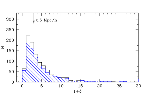
Figure 1: Distribution of the galaxy density contrast for MPGs at 0.5 $\leqslant z\leqslant$ 0.8 with reliable $\delta$ estimates (black solid line). The arrow at the top of the plot is the median value of the distribution with the corresponding value of the projected distance of the fifth nearest neighbor in units of Mpc/h. The solid blue dashed histogram shows the distribution of 1+$\delta$ for the MPGs at 0.5 $\leqslant z\leqslant$ 0.8 with reliable $\delta$ and $R_{e}$ estimates.

Similarly to the $\delta$ estimate, a reliable $R_{e}$ is not available for a small portion of VIPERS galaxies even when the PSF is well modeled. This is either because the algorithm does not converge or because the best-fit values of $n$ $<$ 0.2 are unphysical (see Krywult et al. 2017). These objects were removed from the sample. This choice reduced the sample to 902 MPGs. This is the final sample we used for the MPG $\Sigma$-$\delta$ analysis.

In Fig. 1 the blue histogram shows the local density distribution of the final sample. We verified that the local density distributions of galaxies with and without a reliable $\it{R_{e}}$ measurement are consistent with each other (the Kolmogorov-Smirnov probability that the two distributions shown in Fig. 1 are extracted from the same parent population is 0.99). At the same time, we verified that the lack of a reliable $\delta$ estimate does not depend on $\Sigma$.

For each MPG of the final sample we derived the surface mean stellar mass density $\Sigma.$ Consistently with Paper I, we defined a low-$\Sigma$ sample, an intermediate-$\Sigma$ sample, and a high-$\Sigma$ sample composed of MPGs with $\Sigma\leqslant$ 1000 M_☉ pc^-2, $1000<\Sigma\leqslant$ 2000 M_☉ pc^-2 , and $\Sigma>$ 2000 M_☉ pc^-2, respectively.

We repeat that to study the effect of the environment on the size of the MPGs, we subdivided the sample of MPGs into four subsamples according to the quartiles of the 1+$\delta$ distribution. In Fig. 2 we show the local density $\delta$ of MPGs as a function of $z$ and the 25th, 50th, and 75th percentiles of the 1+$\delta$ distribution at $0.5\leqslant z\leqslant 0.8$ (see Table 1 for the percentile values).

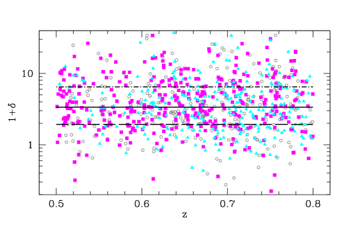
Figure 2: Galaxy density contrast as a function of $z$ for the population of MPGs with reliable estimates of $\delta$ and $\it{R_{e}}$ (gray circles, magenta squares, or cyan triangles). Solid lines indicate the median value of the $(1+\delta)$ distribution, while the 25th and the 75th percentiles are indicated with long-dashed and dot-dashed lines, respectively. Magenta filled squares are MPGs with $\Sigma\leqslant$ 1000 M_☉ pc^-2 (i.e., the low-$\Sigma$ sample), cyan filled triangles are MPGs with $\Sigma>$ 2000 M_☉ pc^-2 (i.e., the high-$\Sigma$ sample) and gray circles are MPGs with 1000 $<\Sigma\leqslant$ 2000 M_☉ pc^-2.

Hereafter, we refer to the four density bins as D1 ($(1+\delta)<$ 25th percentile value), D2 (25th $\leqslant(1+\delta)<$ 50th percentile value), D3 (50th $\leqslant(1+\delta)<$ 75th percentile value), and D4 ($(1+\delta)\geqslant$ 75th percentile value). Most galaxies in the highest density bin (i.e., $(1+\delta)>$ 6.48) are in (small) groups, as shown by Cucciati et al. (2017) (see their Fig. 2). In the same paper, the authors showed that more than 50$\%$ of the galaxies are expected to be central galaxies at our $\mathcal{M}$ scales and redshift range, (see Fig. 8 in Cucciati et al. 2018). This implies that moving from the D1 to D4 density bin, the probability increases that a galaxy assembles stellar mass through the accretion of satellites (through a dry merger or cannibalism).

Table 1: Number of MPGs and 1+$\delta$ percentiles in the full MPG sample and in subsamples subdived by $z$ and $\mathcal{M}$.

	$z$	$N_{tot}$	$N_{D1}$	$N_{D2}$	$N_{D3}$	$N_{D4}$	25th	50th	75th
Total MPG sample
All	0.5 $\leq z\leq$ 0.8	902	226	225	226	225	1.94	3.37	6.48
$\cal{M}$ $\leq$ 2$\times$1011M⊙	0.5 $\leq z\leq$ 0.8	742	186	186	185	185	1.90	3.26	6.18
$\cal{M}$ $>$ 2$\times$1011M⊙	0.5 $\leq z\leq$ 0.8	160	40	40	40	40	2.22	3.94	6.81
Low-$\Sigma$ MPG sample
All	0.5 $\leq z\leq$ 0.8	386	80	102	95	109	1.94	3.37	6.48
$\cal{M}$ $\leq$ 2$\times$1011M⊙	0.5 $\leq z\leq$ 0.8	313	67	84	82	80	1.90	3.26	6.18
$\cal{M}$ $>$ 2$\times$1011M⊙	0.5 $\leq z\leq$ 0.8	73	14	17	17	25	2.22	3.94	6.81
High-$\Sigma$ MPG sample
All	0.5 $\leq z\leq$ 0.8	255	78	56	65	56	1.94	3.37	6.48
$\cal{M}$ $\leq$ 2$\times$1011M⊙	0.5 $\leq z\leq$ 0.8	221	65	48	52	56	1.90	3.26	6.18
$\cal{M}$ $>$ 2$\times$1011M⊙	0.5 $\leq z\leq$ 0.8	34	12	9	10	3	2.22	3.94	6.81
Total MSFG sample
All	0.8 $\leq z\leq$ 1.0	533	134	133	133	133	1.28	2.54	4.27
$\cal{M}$ $\leq$ 2$\times$1011M⊙	0.8 $\leq z\leq$ 1.0	477	120	119	119	119	1.22	2.46	4.28
$\cal{M}$ $>$ 2$\times$1011M⊙	0.8 $\leq z\leq$ 1.0	56	14	14	14	14	2.00	3.11	4.27
Low-$\Sigma$ MSFG sample
All	0.8 $\leq z\leq$ 1.0	398	96	105	95	102	1.28	2.54	4.27
$\cal{M}$ $\leq$ 2$\times$1011M⊙	0.8 $\leq z\leq$ 1.0	360	84	96	85	95	1.22	2.46	4.28
$\cal{M}$ $>$ 2$\times$1011M⊙	0.8 $\leq z\leq$ 1.0	38	10	10	10	8	2.00	3.11	4.27

Column 1: Sample. Column 2: Redshift range. Column 3: Total number of galaxies. Columns 4, 5, 6, and 7: Number of galaxies in the considered sample in the four $\delta$ bins defined according to the 25th, 50th, and 75th percentiles of the (1+$\delta$) distribution. The values of these percentiles are listed in Cols. 8, 9, and 10 for each of the considered samples.

Of the 902 MPGs in the final sample, 386 have $\Sigma\leqslant$ 1000 M_⊙ pc^-2 and 255 have $\Sigma>$  2000M_⊙ pc^-2. The low- (high-) $\Sigma$ subsample can be split into four $\delta$ bins with at least $\sim$ 80(56) galaxies per bin (see Table 1).

3 Galaxy size versus environment at 0.5 ¡ z ¡ 0.8

In Fig.3 we plot the size-mass relation (SMR) of MPGs in the two extreme environments (i.e., MPGs with (1+$\delta$) $\leqslant$ 1.94 and (1+$\delta$) $\geqslant$ 6.48 (D1 and D4 bins, respectively).

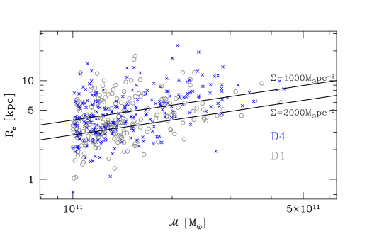
Figure 3: Size-mass relation of MPGs in the lowest (gray open circles) and highest (blue crosses) quartile of (1+$\delta$) distribution (D1 and D4, respectively). The solid lines show the constant mean stellar mass density $\Sigma,$ as annotated.

The figure qualitatively shows that MPGs in the lowest and highest $\delta$ quartiles populate the same locus in the plane. This means that at fixed stellar mass, MPGs with a given $\Sigma$ can be found in any environment. In Appendix B we verify that this result is not dependent on our choice of the $\delta$ values used to identify low- and high-density regions.

This does not tell us whether a given environment can instead favor the formation of a MPG with a given $\Sigma$, however. To address this point, we adopted the following approach. We compared the number of low- and high-$\Sigma$ MPGs in the four local density bins. By construction, each $\delta$ bin contains the same number of MPGs, therefore a constant number of the subpopulations of low- and high-$\Sigma$ MPGs as a function of $\delta$ implies no correlation between $\Sigma$ and $\delta$.

Before we carried this comparison out, we had to apply a correction for the survey incompleteness. VIPERS has three sources of incompleteness: the TSR, the success sampling rate (SSR), and the color sampling rate (CSR). As stated in Sect. 2, the TSR is the fraction of galaxies that are effectively observed with respect to the photometric parent sample. The SSR is the fraction of spectroscopically observed galaxies with a redshift measurement. The CSR accounts for the incompleteness due to the color selection of the survey. These statistical weights depend on the magnitude of the galaxy, on its redshift, color, and angular position. They have been derived for each galaxy in the full VIPERS sample (for a detailed description of their derivation see Garilli et al. 2014; Scodeggio et al. 2018). To correct the number of MPGs in each $\delta$ bin for all of these incompletenesses, we weighted each galaxy $i$ by the quantity w_i = 1/(TSR_i$\times$SSR_i$\times$CSR_i). We do not expect these sources of incompleteness to affect our results because the galaxy size was not considered in the slit assignment in VIPERS. On the other hand, the SSR could be higher for dense MPGs with respect to less dense MPGs because their light profile is more strongly peaked. However, this higher SSR does not depend on the environment because it is only related to the intrinsic properties of the galaxies. The same holds for the CSR. This ensures that the populations of MPGs in dense and less dense environment are not biased in $\Sigma$.

Another factor that can bias our results is the well-known correlation between $\cal{M}$ and $\delta,$ whereby more massive galaxies populate denser environments. We examine the stellar mass distribution of our sample of MPGs as a function of $\delta$ in the upper panel Fig. 4.

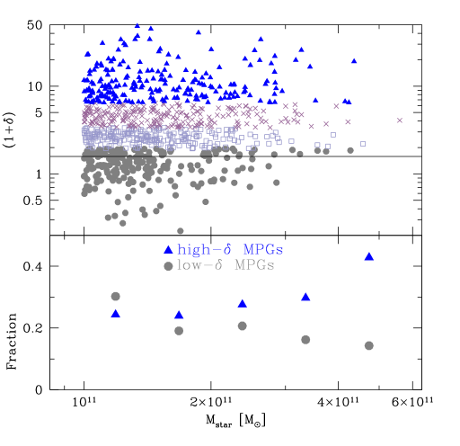
Figure 4: Upper panel: Local density $\delta$ as a function of galaxy stellar mass for our MPG sample. Filled gray circles, open violet squares, pink crosses, and filled blue triangles indicate MPGs in the D1, D2, D3, and D4 quartiles. The horizontal solid line indicates the $\delta$ value above which MPGs cover the full range of stellar mass ($1+\delta=1.5$) (see Sect. 3). Bottom panel: fraction of MPGs in the highest and lowest $\delta$ quartiles as a function of galaxy stellar mass (blue triangles and gray full circles, respectively).

The figure shows that the most massive galaxies are underrepresented in the low-density bin. We quantify this difference in the bottom panel of Fig. 4, where the fraction of MPGs in the lowest and highest $\delta$ quartiles is reported as a function of the stellar mass. In agreement with previous results, we find that the fraction of MPGs in the densest regions increases (by a factor $\sim$2) for stellar masses increasing from 10¹¹ M_⊙ to 5$\times$10¹¹ M_⊙, and concurrently, the fraction of MPGs in the less dense regions decreases with ${\cal M}$.

Figure 3 shows that at higher stellar masses, low-$\Sigma$ MPGs prevail over the full MPG population, resulting in an increasing fraction of low-$\Sigma$ MPGs with $\cal{M}$. This trend, coupled with the $\cal{M}$-$\delta$ correlation shown in Fig. 4, could bias our results toward a false trend of larger galaxies in denser environment.

To remove the possible biases that are due to the different stellar mass distributions of MPGs in low- and high-density regions, we extracted four subsamples of MPGs with the same distribution in stellar mass from the four $\delta$ bins (see Appendix C). This reduced the total number of MPGs to 165 galaxies in each local density quartile.

The filled magenta squares and filled cyan triangles in Fig. 5 indicate the mean number of low- and high-$\Sigma$ MPGs in each $\delta$ bin derived from the 100 mass-matched samples. Error bars take the Poisson fluctuations and the error on the mean into account. Open symbols indicate the same values, but with no correction factor for incompleteness. For both low- and high-$\Sigma$ MPGs, the trend with $\delta$ that is obtained considering the corrected estimates is consistent with the trend obtained with uncorrected estimates. This indicates that the weights we applied do not alter the trends, and it confirms that none of the incompleteness factors depends on $\delta$ or $\Sigma.$ For completeness, we report in Appendix D the same as in Fig. 5, but for the original samples, that is, not mass matched. In the following we refer only to the results obtained with corrected values (filled points in Fig. 5).

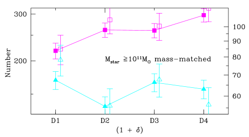
Figure 5: Average number of low-$\Sigma$ (filled magenta squares) and high-$\Sigma$ (filled cyan triangles) MPGs as a function of local density $\delta$ derived from 100 mass-matched samples. The counts are corrected for the selection function of the VIPERS survey. Error bars include the Poisson fluctuations and the error on the mean. The four $\delta$ bins correspond to the four quartiles of the MPG (1+$\delta$) distribution. Open symbols are the mean number of low- and high-$\Sigma$ MPGs that are effectively observed (i.e., not corrected for the selection function) over 100 iterations. The ordinate scale on the right-hand side refers to the uncorrected counts. Light shaded magenta and cyan areas indicate the $\pm$1$\sigma$ region around the mean value of low- and high-$\Sigma$ MPGs that are expected in each bin when no trend with $\delta$ is assumed.

Figure 5 shows similarly to Fig. 3 that low- and high-$\Sigma$ MPGs are ubiquitous in all environments. In addition, it shows that the number of high-$\Sigma$ MPGs is almost constant over the four $\delta$ bins ($\chi^{2}$ = 3.3, the probability $P$ that $\chi^{2}\geqslant$ 3.3 is 0.35). In particular, the number of high-$\Sigma$ MPGs in each $\delta$ bin is consistent within 1$\sigma$ with the mean number derived when no trend with $\delta$ is assumed.

The number of low-$\Sigma$ MPGs slightly and steadily increases from the lowest to the highest $\delta$ quartiles with a $\chi^{2}$ = 8.6 and a probability P($\chi^{2}\geqslant$ 8.6) = 0.035. In particular, the number of low-$\Sigma$ MPGs in the D1 region is more than 1$\sigma$ lower than the number of low-$\Sigma$ MPGs in the D4 region. The difference in the $\delta$ distributions of low- and high-$\Sigma$ MPGs was compared through a Kolmogorov-Smirnov (KS) test. From each mass-matched sample we selected the low- and high-$\Sigma$ MPGs and derived the KS probability $p$ that their $(1+\delta)$ distributions were extracted from the same parent sample. The median value of $p$ over the 100 simulations is 0.11, suggesting that we cannot exclude that the parent population of the two distributions are the same single population. Although the trends we found are marginally significant, they might imply that galaxy size and environment are also related at redshifts 0.5–0.8, and thus it is important to investigate it further.

3.1 Dependence of the $\delta$-$\Sigma$ relation on stellar mass

Several relations involving the stellar mass (e.g., the SMR) show a sharp change in their trends at $\cal{M}$ $\sim$ 2$\times$10¹¹M_⊙ (e.g., Cappellari et al. 2013; Bernardi et al. 2011b, a; Saracco et al. 2017). This feature is interpreted as an indication of an increasing role of satellite accretion in the mass-assembly history of galaxies with stellar mass above such a threshold (Bernardi et al. 2011b, a). According to this picture, we might expect that MPGs with $\cal{M}$ $>$ 2$\times$10¹¹M_⊙ show a stronger positive correlation between their size and the environment than the less massive ones. To test this prediction, we investigated whether the higher number of low-$\Sigma$ MPGs we observe in denser environment is mainly due to galaxies with $\cal{M}$ $>$ 2$\times$10¹¹M_⊙.

In Fig. 6 we report the same analysis as in Fig. 5, but now for MPGs with 10¹¹M_⊙ $\leqslant\cal{M}\leqslant$ 2$\times$10¹¹M_⊙ (lower panel), and with $\cal{M}>$2$\times$10¹¹M_⊙ (upper panel).

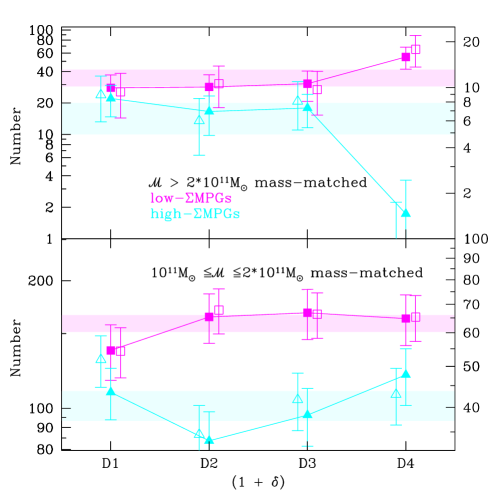
Figure 6: Same as Fig. 5, but for MPGs with 10¹¹M_⊙ $\leqslant\cal{M}\leqslant$ 2$\times$10¹¹M_⊙ (lower panel) and $\cal{M}>$2$\times$10¹¹M_⊙ (upper panel).

The figure shows that, no significant difference in the number of high- and low-$\Sigma$ MPGs with $\delta$ is detectable at lower stellar masses (bottom panel; all the values are consistent at $<1\sigma$ level). At $\cal{M}>$2$\times$10¹¹M_⊙, the numbers of both high- and low-$\Sigma$ MPGs are all consistent in the first three $\delta$ bins, but in the last bin, the number of low-$\Sigma$ MPGs suddenly increases by a factor $\sim$2, while the number of high-$\Sigma$ MPGs drastically drops by a factor $\sim$ 10. The D4 region appears to be lacking high-$\Sigma$ MPGs with $\cal{M}>$2$\times$10¹¹M_⊙, and to have an overabundance of low-$\Sigma$ MPGs with the same stellar mass.

The different $\Sigma$-$\delta$ trends in the two stellar mass bins is also evident in figure 7, where we report for the two stellar mass bins the cumulative distribution of the KS-test probability $p$ that the $(1+\delta)$ distributions of low- and high-$\Sigma$ MPGs from the 100 mass-matched samples are extracted from the same parent population. The figure shows that the median value of $p$ for the high-mass sample is 5$\times$10^-3, and for the low-mass sample is $\sim$0.3. Figures 6 and 7 indicate that the dependence on the environment of low- and high-$\Sigma$ MPGs with $\cal{M}>$ 2$\times$10¹¹M_⊙ is significantly different, with a higher probability to find large (low-$\Sigma$) galaxies in denser environment. Conversely, we do not detect any significant difference in the probability of finding a low- or a high-$\Sigma$ MPG with 10¹¹M_⊙ $\leqslant\cal{M}\leqslant$ 2$\times$10¹¹M_⊙ in a specific environment.

Very few works have investigated the relation between the size/$\Sigma$ and the environment in the same redshift and mass ranges as in this work. Kelkar et al. (2015) find no significant differences in the ${\it R}_{e}$ of red galaxies with $\cal{M}>$ 10¹¹M_⊙ in clusters and fields at $0.4<z<0.8$. This result is partially at odds with our findings because we observe a correlation at the highest mass-scales, but this discrepancy is entirely accounted for by the different observables used in the two analyses. Using their samples, we selected red galaxies on the basis of their $\Sigma$ instead of their ${\it R}_{e}$ and found that the number of low-$\Sigma$ galaxies with $\cal{M}>$ 2$\times$10¹¹M_⊙ in clusters is more than twice the number of low-$\Sigma$ galaxies in the field (9 vs. 4, respectively). This qualitatively agrees with our findings (the number of low-$\Sigma$ MPGs in D4 regions almost doubles the number of low-$\Sigma$ MPGs in D1 regions in this mass range, as shown in the top panel of Fig. 6). Similarly, Lani et al. (2013) measured the local galaxy density in fixed physical apertures of radius 400 kpc and found no dependence between size and environment of quiescent (UVJ selected) galaxies at $0.5<z<1.0$ with $\cal{M}\sim$ 10¹¹M_⊙. At $\cal{M}>$2$\times$10¹¹M_⊙ they found no dependence between the ${\it R}_{e}$ and the environment except for galaxies in the densest regions that are larger than those in other environments. These trends are consistent with the results shown in Fig. 6. Differently from our findings, Huertas-Company et al. (2013a) found no dependence of galaxy size on environment, regardless of stellar mass. In their work, they investigated the ${\it R}_{e}$ - $\delta$ relation for passive and elliptical galaxies, differently from our analysis, which is based on color-selected passive galaxies (as in Lani et al. (2013) and Kelkar et al. (2015)). It is well known that samples of passive galaxies selected through colors contain $20-30\%$ disk galaxies (e.g., Huertas-Company et al. 2013a; Tamburri et al. 2014; Moresco et al. 2013). The different selection method might explain the difference between our MPG sample and their passive galaxy sample, but we are not in the position to quantify the effect of this difference on the results.

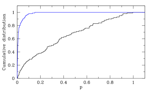
Figure 7: Cumulative distribution of the KS-probability $p$ that the $(1+\delta)$ distributions of low- and high-$\Sigma$ MPGs are extracted from the same parent population that is obtained from all of the 100 mass-matched samples. The black line refers to MPGs with 10¹¹M_⊙ $\leqslant\cal{M}\leqslant$ 2$\times$10¹¹M_⊙, and the blue line to MPGs with $\cal{M}>$ 2$\times$10¹¹M_⊙.

3.2 Relation between $\delta$ and $\Sigma$ for MPGs: summary and discussion

The results we obtained for the mass-matched samples and presented in Figure 6 indicate that

• at 10¹¹M_⊙ $\leqslant\cal{M}\leqslant$ 2$\times$10¹¹M_⊙ we do not observe a significant correlation between the $\Sigma$ of a MPG and the environment in which it lives;

• at $\cal{M}>$2$\times$10¹¹M_⊙ we find a flat trend between the number of low- and high-$\Sigma$ MPGs and $\delta$ in the first three $\delta$ bins. In the highest density bin, the number of low-$\Sigma$ MPGs instead suddenly increases by $\sim$ a factor 2 with respect to the bins at lower density, while the number of high-$\Sigma$ MPGs decreases by a factor $\sim$ 10.

These results indicate that there is no environment that favors (or disfavors) the formation of low- and high-$\Sigma$ MPGs with 10¹¹M_⊙ $\leqslant\cal{M}\leqslant$ 2$\times$10¹¹M_⊙, that is, the mechanisms favored in denser environments, such as satellite accretion or cannibalism, do not appear to be responsible for the low mean surface stellar mass density of large MPGs.

The picture is more complex at higher stellar mass. We observe a decline in the number of high-$\Sigma$ MPGs in the densest environment and concurrently an increase in the number of the low-$\Sigma$ MPGs. This suggests two main scenarios: $i$) the densest environments favor the formation of low-$\Sigma$ MPGs with $\cal{M}>$2$\times$10¹¹M_⊙ and concurrently disfavor the formation of high-$\Sigma$ MPGs with the same stellar mass; $ii$) low- and high-$\Sigma$ MPGs are formed in all environments with the same probability, that is, the formation (at $t=t_{0}$) of dense or not dense passive galaxies does not depend on $\delta$ as for less massive counterparts; but at a later time ($t_{1}>t_{0}$), high-$\Sigma$ MPGs disappear in the most dense regions and low-$\Sigma$ MPGs appear. This means that their evolution does depend on the environment. The hierarchical accretion of satellite galaxies around a compact galaxy could be the driver of a migration of MPGs from the high-$\Sigma$ sample toward the low-$\Sigma$ sample, and consequently be the reason of the abundance (deficit) of low- (high-) $\Sigma$ MPGs with respect to the other $\delta$ bins. Predictions of standard hierarchical models (e.g., Shankar et al. 2012; Huertas-Company et al. 2013a) indicate that at these mass scales, galaxies in groups should be $\sim$ 1.5 times larger than galaxies in less dense fields. We have estimated the mean ${\it R}_{e}$ of MPGs with $\cal{M}>$2$\times$10¹¹M_⊙ in the four density bins and found that it is $\sim$ 1.4 times larger in the D4 bin than in the other less dense environments ($\langle{\it R}_{e}\rangle$ = 6.24$\pm$0.04, 6.18$\pm$0.03, 6.21$\pm$0.03, and 8.73$\pm$0.08 kpc for the D1, D2, D3, and D4 bins, respectively). The concordance between hierarchical model predictions and our observations indicates that accretion of satellites could be a viable mechanisms for the formation and evolution of those largest (e.g., less dense) MPGs with $\cal{M}>$2$\times$10¹¹M_⊙ in excess in the densest regions. This supports the second scenario described above.

Another way to distinguish between the two scenarios would be to investigate the $\Sigma-\delta$ relation for MPGs with $\cal{M}>$2$\times$10¹¹M_⊙ at higher $z$. In the first scenario, we should observe no evolution of the $\Sigma$-$\delta$ relation with time. Conversely, in the second picture, we should observe a flat $\Sigma$-$\delta$ trend at $t=t_{0}$ because the correlation between $\Sigma$ and $\delta$ observed in the top panel of Fig. 6 should appear later, after satellite accretion has become relevant.

Unfortunately, MPGs with $\cal{M}>$ 2$\times$10¹¹M_⊙ at $z>0.8$ are very rare in VIPERS. In spite of the wide coverage of survey, we find only 46 MPGs in the redshift range $0.8<z<0.9$. This prevents an analysis at higher $z$ (we highlight that these 46 MPGs have to be divided into four $\delta$ bins and into low- and high-$\Sigma$ subsamples). Nonetheless, the VIPERS sample offers a unique statistics at $z\geqslant 0.8$ for MSFGs. In Sect. 4 we use the sample of MSFGs at $0.8\leqslant z\leqslant 1.0$ as a benchmark for testing our conclusions.

4 Number of MSFGs as a function of $\delta$

The analysis shown in Fig. 6 questions the relevance of satellite accretion in the mass assembly of low-$\Sigma$ MPGs with 10¹¹M_⊙ $\leqslant\cal{M}\leqslant$ 2$\times$10¹¹M_⊙. Using a different probe (e.g., the number density evolution of MPGs and MSFGs), we reached the same conclusion in Paper I, where we suggested that MSFGs at $z\geqslant 0.8$ are the direct progenitors of low-$\Sigma$ MPGs. If the interpretation we draw based on these two works is correct, we should find that the low-$\Sigma$ MSFGs at $z\geqslant 0.8$ follow the same trend with $\delta$ as low-$\Sigma$ MPGs at $z<$ 0.8 because the former are the progenitors of the latter. To test this hypothesis, we repeated the same analysis as in Sect. 3 for the sample of MSFGs at 0.8 $\leqslant z\leqslant$ 1.0. In this analysis we refer to the density field $\delta$ that is estimated using VIPERS galaxies with M${}_{B}\leqslant$ (-20.9 - $z$) as tracers (see Sec. 2.1). Although this density field is computed on larger scales than the field used for MPGs, it allows us to push the analysis up to $z=1.0$. In Appendix E we show that this choice does not affect our results and conclusions.

In Table 1 we report the total number of MSFGs at 0.8 $\leqslant z\leqslant$ 1.0 with the values of the 25th, 50th, and 75th percentiles of their (1+$\delta$) distribution. As for MPGs, we also report the number of galaxies (and of percentiles) for the two subsamples with 10¹¹M_⊙ $\leqslant\cal{M}\leqslant$ 2$\times$10¹¹M_⊙ and $\cal{M}>$2$\times$10¹¹M_⊙.

In the bottom panel of Fig. 8 we report the number of low-$\Sigma$ MSFGs at 0.8 $\leqslant z\leqslant$ 1.0 with 10¹¹M_⊙ $\leqslant\cal{M}\leqslant$ 2$\times$10¹¹M_⊙ as a function of $\delta$. For comparison, we also report the number of low-$\Sigma$ MPGs at 0.5 $\leqslant z\leqslant$ 0.8, and in the same mass range. In this case, we did not use the mass-matched values, but the values that were just corrected for incompleteness because we are interested in the relative change with $\delta$ of the two populations.

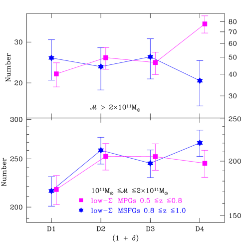
Figure 8: Lower panel: Number of low-$\Sigma$ MSFGs at 0.8 $\leqslant z\leqslant$ 1.0 (blue stars) with 10¹¹M_⊙ $\leqslant\cal{M}\leqslant$ 2$\times$10¹¹M_⊙ as a function of local density $\delta$. For comparison, we also report the number of low-$\Sigma$ MPGs at 0.5 $\leqslant z\leqslant$ 0.8 (magenta squares) with 10¹¹M_⊙ $\leqslant\cal{M}\leqslant$ 2$\times$10¹¹M_⊙. Their values are reported on the right y-axis. The four $\delta$ bins correspond to the four quartiles of the MPG (1+$\delta$) distribution. Upper panel: Same as in the lower panel, but for MPGs with $\cal{M}>$ 2$\times$10¹¹M_⊙

The figure shows that the two trends are consistent at the 1$\sigma$ level. This result, combined with the results in Paper I and Sect. 3, strengthens the postulated evolutionary connection between MSFGs and MPGs. In Paper I we demonstrated that MSFGs at $z\sim 0.8$ are in the correct number to be the progenitors of low-$\Sigma$ MPGs at $z<0.8$, and here we show that they are also in the correct environment. The analyses of the number density and of the environment concur in indicating that low-$\Sigma$ MPGs with 10¹¹M_⊙ $\leqslant\cal{M}\leqslant$ 2$\times$10¹¹M_⊙ at $z<0.8$ are the descendants of MSFGs at higher $z$ and not the result of satellite accretion.

In Sect. 3.2 we have shown that the accretion of satellites could be a viable mechanisms for the formation of the exceedingly low-$\Sigma$ MPGs with $\cal{M}>$ 2$\times$10¹¹M_⊙ in the D4 bin. In this picture, the $\Sigma$-$\delta$ trend of low-$\Sigma$ MPGs at $z<0.8$ should not be consistent with that of MSFGs at $0.8<z<1.0$, as we found for lower mass-scales. The two trends are expected to deviate in the highest density bin because the majority of MSFGs become passive at $z<0.8,$ but to these ”shutdown” MPGs we should add in the highest density bin the large MPGs that are formed by the accretion of satellites.

In the top panel of Fig. 8 we report the $\Sigma$ - $\delta$ trend for MSFGs with $\cal{M}>$ 2$\times$10¹¹M_⊙. It shows that in the highest stellar mass bin, the $\Sigma$ - $\delta$ trend for MSFGs at $z>0.8$ is flat (all points are consistent within 1$\sigma$). We observe instead a flat $\Sigma$ - $\delta$ trend for MPGs at $z<0.8$ in the first three $\delta$ bins and an increase in the number of low-$\Sigma$ MPGs in the highest density bin (see the magenta points in the upper panel of Fig. 8). This evidence supports the second scenario we proposed in Sect. 3.2. The flat trend of MSFGs over the four $\delta$ bins indicates that at $t=t_{0}$, the probability that a MSFG with $\cal{M}>$ 2$\times$10¹¹M_⊙ (and consequently of its descendant MPG) has a low-$\Sigma$ is independent of the environment. At $t_{1}>t_{0}$, environment-related mechanisms, such as accretion of satellites, are responsible for the surplus of MPGs that is observed in the D4 bin.

In summary, our analysis shows that the larger size of most of the low-$\Sigma$ MPGs is not a consequence of a hierarchical assembly of the stellar matter. Although this is true for the majority of the galaxies in our sample, we cannot rule out satellite accretion as one of the main mechanisms responsible for increasing the size, thus decreasing $\Sigma$, in a small fraction of high-$\Sigma$ MPGs with $\cal{M}>$2$\times$10¹¹M_⊙ that reside in the densest environments (i.e., $\sim$ 10 high-$\Sigma$ MPGs over $\sim$902, where 10 is the difference between the mean value of high-$\Sigma$ MPGs in the D1, D2, and D3 bins and the value in the D4 bin, see the upper panel of Fig. 6, and 902 is the total number of MPGs).

5 Summary

Using the VIPERS spectroscopic survey, we investigated the relation between the typical size of MPGs and their environment. In a hierarchical scenario, structures are expected to grow in mass and size through accretion of smaller units. The accretion of satellites is enhanced in groups (and for central galaxies), thus we would expect to find larger galaxies in groups than in less dense environments. The study of galaxy sizes as a function of the environment therefore is a powerful diagnostic for galaxy accretion models.

From the VIPERS database we extracted all the galaxies at 0.5 $\leqslant z\leqslant$ 0.8 with $\cal{M}\geqslant$ 10¹¹M_⊙. From these systems we selected the passive galaxies according to their NUV$r$K colors. The sample is 100$\%$ complete in stellar mass at $z=0.8.$ From the massive and passive galaxies, we selected those with reliable estimates of the effective radius $\it{R_{e}}$ and of the galaxy density contrast $\delta$. This led to a total final sample of 902 MPGs in the redshift range 0.5 $\leqslant z\leqslant$ 0.8.

From this sample, we selected a low-$\Sigma$ subsample composed of MPGs with a mean surface stellar mass density $\Sigma\leqslant$ 1000 Mpc pc^-2, and a high-$\Sigma$ subsample that contains the MPGs with $\Sigma>$ 2000 Mpc pc^-2.

The overall picture we obtained from our analysis of size versus environment in VIPERS galaxies at $0.5\leqslant z\leqslant 0.8$ is described below.

• The $\Sigma$-$\delta$ relation depends on stellar mass. In particular, MPGs with 10¹¹M_⊙ $\leqslant\cal{M}\leqslant$ 2$\times$10¹¹M_⊙ do not show any significant trend between the $\Sigma$ (or equivalently $\it{R_{e}}$) and the environment (the KS probability $p$ that the density contrast distributions of low- and high-$\Sigma$ MPGs are extracted by the same parent sample is 0.3, see Fig. 7), while a significant correlation is detected for MPGs with $\cal{M}>$ 2$\times$10¹¹M_⊙ ($p=5\times 10^{-3}$), with larger galaxies being more common in denser environments.

• The trend between $\Sigma$ and $\delta$ observed for MPGs with $\cal{M}>$ 2$\times$10¹¹M_⊙ is due to an overabundance of low-$\Sigma$ MPGs and by a dearth of high-$\Sigma$ MPGs in the densest regions (see Fig. 6).

The absence of a correlation between $\Sigma$ and $\delta$ for MPGs with 10¹¹M_⊙ $\leqslant\cal{M}\leqslant$ 2$\times$10¹¹M_⊙ indicates that the accretion of satellite galaxies is not the main driver of the build-up of low-$\Sigma$ MPGs in this stellar mass range. This result is in line with our previous results. In Paper I (see Fig. 9), the analysis of the number densities of MPGs and MSFGs suggested that the most plausible progenitors of the emerging low-$\Sigma$ MPGs at $z<0.8$ are the MSFGs at $z>0.8$. We further investigated this connection and in Fig. 8 compared the $\Sigma-\delta$ trends for MSFGs at $z>0.8$ and low-$\Sigma$ MPGs $z<0.8$. The two trends are consistent at the 1$\sigma$ level, as it should be if the two populations are evolutionary connected. In Paper I we demonstrated that the MSFGs are in the correct number to be the progenitors of low-$\Sigma$ MPGS, and here we show that they are also in the correct environment.

For the highest stellar mass bin, our results on the $\Sigma$-$\delta$ correlation of both MPGs and MSFGs are consistent with a scenario in which, overall, environment does not affect the formation of low- or high-$\Sigma$ MPGs. Nonetheless, it seems to play a relevant role in the evolution of a small fraction ($<1\%$) of low-$\Sigma$ MPGs in the densest environment. We interpret the increased number of low-$\Sigma$ MPGs in the densest regions as a consequence of a migration of high-$\Sigma$ MPGs in low-$\Sigma$ MPGs that is due to accretion of satellite galaxies. These results are also confirmed by comparison with predictions of hierarchical models.

Appendix A $\delta$ distribution as a function of $z$

In this section we investigate the dependence of the (1+$\delta$) distribution of MPGs on $z$. In Fig. 9 we plot the cumulative distributions of the local density for MPGs with reliable $\it{R_{e}}$ and $\delta$ in the two different redshift bins 0.5 $\leqslant z\leqslant$ 0.8 and 0.8 $<z\leqslant$ 0.9. The KS test indicates a probability $p$ = 0.07 that the two distributions are extracted from the same parent sample. Conversely, we do not find a strong dependence between $z$ and the $\delta$ distributions at $z\leqslant 0.8$. As an example, the red lines in Fig. 9 indicate the (1+$\delta$) distribution for MPGs in the redshift bins 0.5 $\leqslant z\leqslant$ 0.6 and 0.7 $\leqslant z\leqslant$ 0.8. The probability that the two distributions are extracted from the same parent sample is $p$ = 0.64.

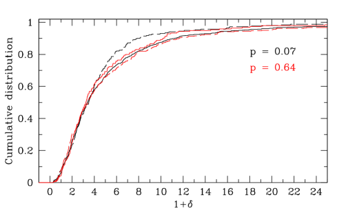
Figure 9: Cumulative distribution of (1+$\delta$) for MPGs with reliable $\it{R_{e}}$ and $\delta$ at 0.5 $\leqslant z\leqslant$ 0.8 (black solid line) and at 0.8 $<z\leqslant$ 0.9 (dashed black line). The probability $p$ that the two distributions are extracted from the same parent sample is rejected at $\sim$3$\sigma$. Red solid and dashed lines indicate the cumulative distribution for MPGs at 0.5 $\leqslant z\leqslant$ 0.6 and 0.7 $\leqslant z\leqslant$ 0.8, respectively. The probability that they are extracted from the same parent sample is 0.64.

Appendix B Effect of the environment on the stellar mass distribution

In this section we investigate the size-mass relation in two extreme environments. In particular, we report the size-mass relation for MPGs with (1+$\delta$) $\leqslant$ 1.5 and $(1+\delta)$ $\geqslant$ 7 (see Fig. 4 and the text for the choice of these new cuts). We find that MPGs in regions with $(1+\delta)$ $\geqslant$ 7 populate similar regions in the $\it{R_{e}}$ versus $\cal{M}$ plane of MPGs with $(1+\delta)$ $\geqslant$ 6.48 (see the filled and open blue points in Fig. 10). Conversely, the population of MPGs with (1+$\delta$) $\leqslant$ 1.5 does not include the most massive galaxies with respect to the population of MPGs with (1+$\delta$) $\leqslant$ 1.94.

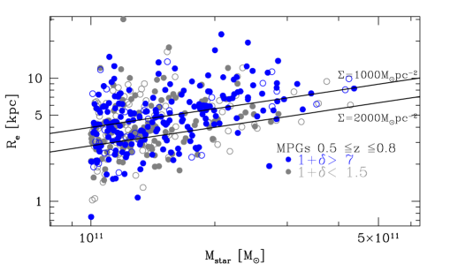
Figure 10: Size-mass relation of MPGs in the final sample with (1+$\delta$) $<$ 1.5 (gray filled circles) and with (1+$\delta$) $>$ 7 (blue filled circles). Open blue and gray circles are the MPGs that were excluded from Fig. 3, i.e., MPGs with 1.5 $\leqslant(1+\delta)\leqslant$ 1.94 and 6.48 $\leqslant(1+\delta)\leqslant$ 7, respectively.

Despite the lack of massive galaxies in the lowest density regions, Fig. 10 shows that in the stellar mass range covered both by MPGs with $(1+\delta)$ $<$ 1.5 and by MPGs with $(1+\delta)$ $>$ 7 (i.e., $\cal{M}<$3$\times$10¹¹ M_⊙) the range of $\it{R_{e}}$ that is covered is not significantly different. This indicates that environment plays an important role in setting the stellar mass (we take this aspect into account in Sect. 3.2), as is known, but it confirms that our results shown in Fig. 3 are robust against the choice of the $\delta$ cuts.

Appendix C Construction of the mass-matched samples

To construct the mass-matched samples we used in the analysis of Sect. 3, we started from the samples of MPGs in the four $\delta$ bins. We subdivided the four samples into bins of 0.05dex in stellar mass. For any stellar mass bin, we identified the sample with the lowest number of objects, and then randomly extracted from the others an equal number of galaxies. The stellar mass distributions of MPGs in the four $\delta$ bins and the stellar mass distribution of a mass-matched sample are shown in Fig. 11.

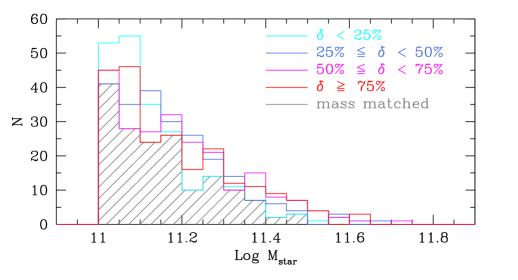
Figure 11: Stellar mass distribution of MPGs at 0.5 $\leqslant z\leqslant$ 0.8 in the four $\delta$ bins (cyan, blue, magenta, and red histograms for the D1, D2, D3, and D4 $\delta$ bin, respectively). The dashed gray histogram indicates the stellar mass distribution of the mass-matched sample.

Appendix D Number of MPGs as a function of $\Sigma$ and $\delta$ for the not mass-matched samples

In Figs. 5 and 6 in Sect. 3 we report the number of MPGs as a function of their $\Sigma$ and $\delta$ for the mass-matched samples. In this appendix we show the results for the original samples. In Fig. 12 filled points show the numbers of low- and high-$\Sigma$ MPGs in the four $\delta$ bins, corrected for the TSR, SSR, and CSR incompleteness factors. Open magenta and cyan points show the same, but without the completeness correction factors.

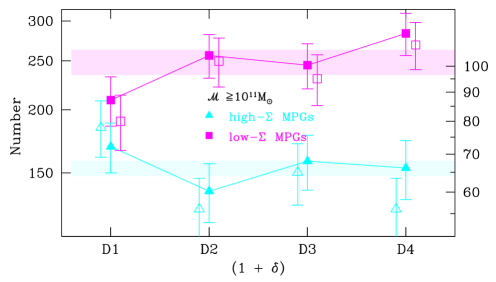
Figure 12: Same as Fig. 5, but now the filled magenta and cyan symbols show the number of low-$\Sigma$ and high-$\Sigma$ MPGs corrected for the selection function of the VIPERS survey. Error bars take the Poisson fluctuations into account. Open symbols show the number of low- and high-$\Sigma$ MPGs that are effectively observed (i.e., not corrected for the selection function).

In Fig. 13 we show the number of low- and high-$\Sigma$ MPGs as a function of $\delta$ as in Fig. 12, but for the two subsamples of MPGs with 10¹¹M_⊙ $\leqslant\cal{M}\leqslant$ 2$\times$10¹¹M_⊙ (bottom panel) and with $\cal{M}>$ 2$\times$10¹¹M_⊙ (upper panel).

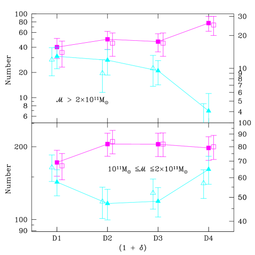
Figure 13: Same as Fig.12, but for the two bins of stellar mass.

Overall, the trends we found is similar to the trends derived for the mass-matched samples.

Appendix E Negligible effect of the density field definition on our conclusions.

In this section we show that the choice of the density fields does not affect our conclusions. In Fig. 14 the filled magenta squares show the number density of low-$\Sigma$ MPGs with 10¹¹M_⊙ $\leqslant\cal{M}\leqslant$ 2$\times$10¹¹M_⊙ as a function of $\delta$, where $\delta$ is computed using as tracer galaxies with M${}_{B}\leqslant$ (-20.4 - $z$) (i.e., this is the same as in Fig. 8). Open magenta squares show the same, but for $\delta$ derived using VIPERS galaxies with M${}_{B}\leqslant$ (-20.9 - $z$) as tracers. The figure shows that the two functions are in agreement within the errors.

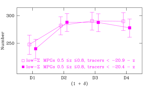
Figure 14: Number of low-$\Sigma$ MPGs as a function of $\delta$ in the case the density field is estimated using galaxies with M${}_{B}<$ $-20.4-z$ as tracers (filled magenta squares) and when galaxies with M${}_{B}<$ $-20.9-z$ were used.