Matching Estimators with Few Treated and Many Control Observations

We analyze the properties of matching estimators when there are few treated, but many control observations. We show that, under standard assumptions, the nearest neighbor matching estimator for the average treatment effect on the treated is asymptotically unbiased in this framework. However, when the number of treated observations is fixed, the estimator is not consistent, and it is generally not asymptotically normal. Since standard inference methods are inadequate, we propose alternative inference methods, based on the theory of randomization tests under approximate symmetry, that are asymptotically valid in this framework. We show that these tests are valid under relatively strong assumptions when the number of treated observations is fixed, and under weaker assumptions when the number of treated observations increases, but at a lower rate relative to the number of control observations.

Keywords: matching estimators, treatment effects, hypothesis testing, randomization inference, synthetic control estimator

JEL Codes: C12; C13; C21

1 Introduction

Matching estimators have been widely used for the estimation of treatment effects under a conditional independence assumption (CIA). In many cases, matching estimators have been applied in settings where (1) the interest is on the average treatment effect for the treated (ATT), and (2) there is a large reservoir of potential controls (see Imbens and Wooldridge, (2009)). Abadie and Imbens, (2006) (henceforth, AI) study the asymptotic properties of nearest-neighbor (NN) matching estimators when the number of control observations ($N_{0}$) grows at a faster rate than the number of treated observations ($N_{1}$). However, their asymptotic theory still depends on both the number of treated and control observations going to infinity. Therefore, reliance on such asymptotic approximation should be considered with caution when the number of treated observations is small, even if the total number of observations is large.

In this paper, we analyze the properties of NN matching estimators when $N_{1}$ is fixed, while $N_{0}$ goes to infinity. We first show that the NN matching estimator is asymptotically unbiased for the ATT, under standard assumptions used in the literature on estimation of treatment effects under selection on observables. This is consistent with the conclusions from AI, who show that the conditional bias of the NN matching estimator can be ignored, provided that $N_{0}$ increases fast enough, relative to $N_{1}$. In their setting, the NN matching estimator is consistent and asymptotically normal. In our setting, however, the variance of the estimator does not converge to zero, and the estimator will not generally be asymptotically normal. Our theory complements the theory developed by AI, providing a better approximation to settings in which there is a larger number of control relative to treated observations, but $N_{1}$ is not large enough, so that we cannot rely on asymptotic results in which $N_{1}$ goes to infinity.

The fact that the NN matching estimator is not asymptotically normal, in our setting, poses important challenges when it comes to inference. Inference based on the asymptotic distribution of the matching estimator derived by AI should not provide a good approximation when $N_{1}$ is very small, even if there are many control observations. The bootstrap procedure proposed by Otsu and Rai, (2017) also relies on the number of both treated and control observations going to infinity. Hong et al., (2019) consider a finite population setting with limited overlap, where the probability of treatment may converge to zero for some strata. While they provide conditions in which standard inference methods remain asymptotically valid in this case, our setting with $N_{1}$ fixed would not satisfy their conditions. Rothe, (2017) provides robust confidence intervals for average treatment effects under limited overlap. For the case with continuous covariates, he combines his method with subclassification on the propensity score. However, with few treated and many control observations, it would not be possible to reliably estimate a propensity score. Moreover, while Armstrong and Kolesár, (2021) propose confidence intervals that are asymptotically valid even when $\sqrt{n}-$inference is not possible, the conditions they consider for this result are not satisfied in our setting. Finally, for finite samples, Rosenbaum, (1984) and Rosenbaum, (2002) consider permutation tests for observational studies under strong ignorability. However, these tests rely on restrictive assumptions.

Given the limitations of existing inference methods for the setting we analyze, we consider alternative inference methods based on the theory of randomization tests under an approximate symmetry assumption, developed by Canay et al., (2017). We focus on a test based on sign changes. We show that, under symmetry assumptions on the errors and on the heterogeneous treatment effects, this test provides asymptotically valid hypothesis testing for the ATT when $N_{0}\rightarrow\infty$, even when $N_{1}$ is fixed. When $N_{1}$ increases, but at a lower rate than $N_{0}$, we show that this test is asymptotically valid even when we relax such symmetry conditions. Therefore, this test works with very few treated observations under relatively strong assumptions, and with a larger number of treated observations under weaker assumptions. We consider in Appendix LABEL:Section_permutation an alternative test based on permutations, which also has the property of being valid under stronger assumptions when $N_{1}$ is fixed, and under weaker assumptions when $N_{1}$ increases.

The remainder of this paper proceeds as follows. We present our theoretical setup in Section 2. In Section 3, we derive the asymptotic distribution of the NN matching estimator, and derive conditions under which it is asymptotically unbiased in a setting with fixed $N_{1}$. In Section 4, we consider an alternative inference method that is asymptotically valid when $N_{0}\rightarrow\infty$, while $N_{1}$ remains fixed. We also consider the properties of this test when $N_{1}$ increases. In Section 5, we present Monte Carlo (MC) simulations. In Section 6, we contrast the different inference procedures in light of the theoretical results presented in Section 4 and the simulations presented in Section 5, providing guidance on which method should be chosen depending on the setting. We present in Section 7 an empirical illustration based on the “Jovem de Futuro” program, which provides an example in which matching estimators could be used in settings with few treated and many control observations. Concluding remarks, including a discussion on the implications of our results for other types of matching estimators and for Synthetic Control applications, are presented in Section 8.

2 Setting and Notation

We are interested in estimating the effect of a binary treatment ($W$) on some outcome ($Y$). Following Rubin, (1973), we define $Y(0)$ as the potential outcome under no exposure to treatment, and $Y(1)$ as the potential outcome under exposure to treatment. Therefore, the observed outcome is given by $Y=WY(1)+(1-W)Y(0)$. In addition to $Y$ and $W$, we also consider a continuous random vector of $k$ real-valued pretreatment variables, which we denote by $X$.

We observe $N_{1}$ treated observations obtained by random sampling from the distribution of $(Y,X)|W=1$ and $N_{0}$ untreated observations obtained by random sampling from the distribution of $(Y,X)|W=0$. Let $\mathcal{I}_{w}$ denote the set of indexes for observations with $W_{i}=w$.

Assumption 2.1 (Sample)

$\{Y_{i},X_{i},W_{i}\}_{i\in\mathcal{I}_{1}\cup\mathcal{I}_{0}}$ is a pooled sample of $N_{1}$ treated ($i\in\mathcal{I}_{1}$) and $N_{0}$ untreated ($i\in\mathcal{I}_{0}$) observations obtained by random sampling from their respective population counterparts. Furthermore, observations in the treated and control samples are independent.

We consider the case in which $N_{1}$ is fixed, while $N_{0}$ goes to infinity. One possibility is that there is a large set of units that could potentially be treated, but only a finite number of them actually receive treatment. For example, in the empirical application, to be presented in Section 7, there is a large number of schools that could potentially receive the treatment, but only a small number of them actually received it. Alternatively, we can imagine that there is a large number of treated units, but we only have data from a small sample of them. Assumption 2.1 is similar to Assumption 3^′ from AI and from the first condition stated in Theorem 1 from Abadie and Imbens, (2012), in that the proportions of treated and control observations in the sample may not reflect their proportions in the population.

The goal is estimating the ATT, which we denote by

$$\tau\equiv\mathbb{E}\left[Y(1)-Y(0)|W=1\right].$$ (1)

We focus on an estimand related to the treatment effect on the treated because, given our setting with $N_{1}$ finite and $N_{0}$ large, we would only have a small number of treated observations to serve as potential neighbors to estimate the counterfactual of the control observations, in case we wanted to estimate the average treatment effect (ATE). Likewise, AI consider the estimation of the ATT when they consider an asymptotic framework in which $N_{0}$ grows at a faster rate than $N_{1}$. In Appendix LABEL:Appendix_CATT we discuss the case in which the estimand of interest is the ATT conditional on the realization of the covariates for the treated observations, $\{X_{i}\}_{i\in\mathcal{I}_{1}}$.

Assumption 2.1 does not impose any restriction on how the distribution of $(Y(1),Y(0),X)$ conditional on $W=w$ depends on $w$. The following assumption restricts the way in which these distributions may differ, which is a standard conditional independence assumption (CIA).

Assumption 2.2 (Conditional Independence Assumption)

$Y(0)\perp\!\!\!\perp W|X$.

While Assumption 2.2 restricts that the conditional distribution of $Y(0)$ given $X$ is the same for both treatment and control observations, the density of $X$ conditional on $W=w\in\{0,1\}$ can potentially depend on $w$. This is what potentially generates bias in a simple comparison of means between treated and control groups, without taking into account that these groups might have different distributions of covariates $X$. We do not need to impose conditional independence of $Y(1)$ because the focus is on the ATT, and not on the average treatment effects.

The next assumption states conditions on the distribution of the covariates. Let $\mathbb{X}_{w}$ be the support of $X$ conditional on $W=w$, and $f_{w}:\mathbb{X}_{w}\rightarrow\mathbb{R}_{+}$ be the conditional density of $X$ given $W=w$, for $w\in\{0,1\}$.

Assumption 2.3 (Distribution of covariates)

(i) $X\in\mathbb{R}^{k}$ is an absolutely continuous random vector, (ii) $\mathbb{X}_{1}\subseteq\mathbb{X}_{0}$, where $\mathbb{X}_{1}$ and $\mathbb{X}_{0}$ are compact, (iii) $f_{1}$ and $f_{0}$ are differentiable for all points in the interior of their support, bounded from above in $\mathbb{X}_{1}$, and $f_{0}$ is bounded from below in $\mathbb{X}_{1}$, and (iv) for all points in $x\in\mathbb{X}_{1}$ at least a fraction $\phi$ of any sphere around $x$ belongs to $\mathbb{X}_{1}$.

This assumption guarantees that, for each $i$ in the treated group, we can find an observation $j$ in the control group with covariates $X_{j}$ arbitrarily close to $X_{i}$ when $N_{0}\rightarrow\infty$. As we show in Appendix LABEL:proof_sign_changes_asympt, Assumption 2.3 implies that there is an $\eta>0$ such that, for all $x\in\mathbb{X}_{1}$, $Pr(W=1|X=x)<1-\eta$.

The main identification problem arises from the fact that we observe either $Y_{i}(1)$ or $Y_{i}(0)$ for each observation $i$. If we had two observations, $i\in\mathcal{I}_{1}$ and $j\in\mathcal{I}_{0}$, with $X_{i}=X_{j}=x$, then, under Assumptions 2.1 and 2.2, $\mathbb{E}[Y_{i}|X_{i}=x]-\mathbb{E}[Y_{j}|X_{j}=x]=\mathbb{E}[Y(1)|W=1,X=x]-\mathbb{E}[Y(0)|W=0,X=x]=\mathbb{E}[Y(1)-Y(0)|X=x,W=1]$. The main challenge is that, with a continuous random variable $X$, the probability of finding treated and control observations with exactly the same $X$ is zero. The idea of the NN matching estimator is to input the missing potential outcome of a treated observation $i\in\mathcal{I}_{1}$ with observations from the control group $j\in\mathcal{I}_{0}$ that are as close as possible in terms of covariates $X_{i}$. More specifically, for a distance metric $d(a,b)$ in $\mathbb{R}^{k}$, let $\mathcal{J}_{M}(i)$ be the set of $M$ nearest neighbors in the control group of observation $i\in\mathcal{I}_{1}$. Then the NN matching estimator is given by

$$\hat{\tau}=\frac{1}{N_{1}}\sum_{i\in\mathcal{I}_{1}}\left[Y_{i}-\frac{1}{M}\sum_{j\in\mathcal{J}_{M}(i)}Y_{j}\right],$$ (2)

where we consider the matching estimator with replacement. We consider the case in which $d(a,b)=[(a-b)^{\prime}V(a-b)]^{1/2}$ for some positive definite matrix $V$. In Remark LABEL:Mahalanobis in the appendix we show that our results are also valid if we consider the Mahalanobis distance.

3 Asymptotic Unbiasedness and Asymptotic Distribution

For $w\in\{0,1\}$, we define $\mu(x,w)=\mathbb{E}[Y|X=x,W=w]$ and $\epsilon=Y-\mu(X,W)$. Since we are focusing on the average treatment effect on the treated, we also define $\mu_{w}(x)=\mathbb{E}[Y(w)|X=x,W=1]$. Under Assumption 2.2, we have that $\mu(x,0)=\mu_{0}(x)$. Using this notation, the ATT is given by

$$\tau=\mathbb{E}\left[\mu_{1}(X)-\mu_{0}(X)|W=1\right],$$ (3)

and the NN matching estimator is given by

$$\hat{\tau}=\frac{1}{N_{1}}\sum_{i\in\mathcal{I}_{1}}\left[\left(\mu_{1}(X_{i})-\frac{1}{M}\sum_{j\in\mathcal{J}_{M}(i)}\mu_{0}(X_{j})\right)+\left(\epsilon_{i}-\frac{1}{M}\sum_{j\in\mathcal{J}_{M}(i)}\epsilon_{j}\right)\right].$$ (4)

We first show that $\hat{\tau}$ is an asymptotically unbiased estimator for the ATT when $N_{1}$ is fixed and $N_{0}\rightarrow\infty$, and we derive its asymptotic distribution in this setting. We consider the following assumptions on how the distribution of $Y(0)|X=x$ changes with $x$.

Assumption 3.1 (Distribution of $Y(0)|X=x$)

(a) $\mu_{0}(x)$ is continuous, and (b) for any $h(y)$ continuous and bounded, $\tilde{h}(x)=\mathbb{E}[h(Y(0))|X=x]$ is continuous and bounded.

Assumption 3.1(a) states that the conditional expectation of $Y(0)$ with respect to $X=x$ is continuous in $x$, which is standard in the matching literature. The intuition behind Assumption 3.1(b) is that the conditional distribution of $Y(0)$ given $X=x$ changes “smoothly” with $x$. This guarantees that $Y(0)|(X=x_{n})$ converges in distribution to $Y(0)|(X=x)$ if $x_{n}\rightarrow x$, as we show in Appendix Lemma LABEL:Lemma_convergenceY. In Appendix LABEL:condition_normal, we show that this condition is satisfied if, for example, $Y(0)|(X=x)\sim N(\theta(x),\sigma(x))$, where $\theta(x)$ and $\sigma(x)$ are continuous functions of $x$.

For each $x\in\mathbb{X}_{1}$, let $\xi_{x}\sim(Y(1)-\mu_{1}(x))|(X=x,W=1)$ and $\eta_{x}\sim(Y(0)-\mu_{0}(x))|(X=x,W=0)$. Moreover, let $G(\kappa;x)$ be the CDF of $(\mu_{1}(x)-\mu_{0}(x)-\tau)+\xi_{x}-\frac{1}{M}\sum_{m=1}^{M}\eta_{x}^{m}$, where $\{\eta_{x}^{m}\}_{m=1}^{M}$ are iid copies of $\eta_{x}$, and $(\xi_{x},\eta^{1}_{x},\cdots,\eta^{M}_{x})$ is mutually independent.

Proposition 3.1

(1) Under Assumptions 2.1, 2.2, 2.3, and 3.1(a), $\mathbb{E}[\hat{\tau}]\rightarrow\tau$ when $N_{0}\rightarrow\infty$ and $N_{1}$ is fixed.

(2) Under Assumptions 2.1, 2.2, 2.3, and 3.1(b),

$$\hat{\tau}\buildrel d\over{\rightarrow}\tau+\frac{1}{N_{1}}\sum_{i\in\mathcal{I}_{1}}\kappa_{i}\mbox{ when $N_{0}\rightarrow\infty$ and $N_{1}$ is fixed},$$

where the CDF of $\kappa_{i}$ is given by $\widetilde{G}(\kappa)=\int_{x\in\mathbb{X}_{1}}G(\kappa;x)f_{1}(x)dx$, and $\mathbb{E}[\kappa_{i}]=0$. Moreover, $\{\kappa_{i}\}_{i\in\mathcal{I}_{1}}$ is mutually independent.

Let $X^{i}_{(m)}$ be the covariate value of the $m$-closest match to observation $i\in\mathcal{I}_{1}$. The main intuition for the results in Proposition 3.1 is that, for a fixed $X_{i}=\bar{x}$, $X^{i}_{(m)}\buildrel p\over{\rightarrow}\bar{x}$ when $N_{0}\rightarrow\infty$, because, holding $M$ fixed, we will always be able to find $M$ observations in the control group that are arbitrarily close to $\bar{x}$. Independence of $\kappa_{i}$ follows from the fact that the probability of two treated observations sharing the same nearest neighbor converges to zero. See details in Appendix LABEL:proof_unbiased.

Proposition 3.1 shows that the expected value of the NN matching estimator converges to $\tau$. We also derive in Proposition 3.1 the asymptotic distribution of $\hat{\tau}$, which has expected value equal to $\tau$. Therefore, the NN matching estimator is asymptotically unbiased whether we define asymptotic unbiasedness as $\mathbb{E}[\hat{\tau}]\rightarrow\tau$, or as $\hat{\tau}\buildrel d\over{\rightarrow}\tau+\widetilde{\kappa}$, with $\mathbb{E}[\widetilde{\kappa}]=0$.

Remark 3.1

With $N_{1}$ fixed, the estimator is not consistent. This happens because, with $N_{1}$ fixed, we cannot apply a law of large numbers to the average of the error of the treated observations. For the same reason, the matching estimator will not generally be asymptotically normal. These conclusions are similar to the ones derived by Conley and Taber, (2011) for differences-in-differences estimators with few treated groups.

Remark 3.2

Consider a bias-corrected estimator suggested by Abadie and Imbens, (2011),

$$\hat{\tau}_{biasadj}=\frac{1}{N_{1}}\sum_{i\in\mathcal{I}_{1}}\left[Y_{i}-\frac{1}{M}\sum_{m=1}^{M}\left(Y_{j}+\hat{\mu}_{0}(X_{i})-\hat{\mu}_{0}(X^{i}_{(m)})\right)\right],$$ (5)

where $\hat{\mu}_{0}(x)$ is an estimator for $\mu_{0}(x)$, and $X^{i}_{(m)}$ be the covariate value of the $m$-closest match to observation $i$. If the conditions on $\hat{\mu}_{0}(x)$ considered by Abadie and Imbens, (2011) are satisfied, then we can also guarantee that $\hat{\tau}_{biasadj}$ has the same asymptotic distribution as $\hat{\tau}$. The intuition is that $\hat{\mu}_{0}(X_{i})-\hat{\mu}_{0}(X^{i}_{(m)})$ converges in probability to zero when $N_{0}\rightarrow\infty$, because $X^{i}_{(m)}\buildrel p\over{\rightarrow}X_{i}$.

Remark 3.3

We consider an asymptotic framework in which $M$ is held fixed, while $N_{0}\rightarrow\infty$, which is similar to what AI call fixed-$M$ asymptotics in their setting. As argued by AI, the motivation for such fixed-$M$ asymptotics is to provide an approximation to the sampling distribution of matching estimators with a small number of matches. Matching estimators using few matches have been widely used in applied work (see AI). Moreover, Imbens and Rubin, (2015) argue against using matching estimators with many matches, as this would tend to increase the bias of the resulting estimator, while the marginal gains in precision of increasing the number of matches are limited. In Section 8 we consider the implication of our findings for other types of matching estimators.

4 Inference

The fact that the NN matching estimator is not generally asymptotically normal when $N_{1}$ is fixed and $N_{0}\rightarrow\infty$ poses an important challenge when it comes to inference. In particular, inference based on the asymptotically normal distribution derived by AI, or on the bootstrap procedure suggested by Otsu and Rai, (2017), should not provide a good approximation in our setting, as the asymptotic theory behind these methods relies on both $N_{1}$ and $N_{0}$ going to infinity. We therefore consider alternative inference methods based on the theory of randomization tests under an approximate symmetry assumption, developed by Canay et al., (2017). We focus on a test based on sign changes, while in in Appendix LABEL:Section_permutation we consider an alternative test based on permutations. We consider the problem of testing the null hypothesis $H_{0}:\tau=c$.

Without loss of generality, let $i=1,...,N_{1}$ be the treated observations, and consider a function of the data given by

$$S_{N_{0}}=\left(\hat{\tau}_{1}^{N_{0}},...,\hat{\tau}_{N_{1}}^{N_{0}}\right)^{\prime}$$ (6)

where $\hat{\tau}_{i}^{N_{0}}=\left(Y_{i}-\frac{1}{M}\sum_{j\in\mathcal{J}_{M}(i)}Y_{j}\right)-c$. Each $\hat{\tau}_{i}^{N_{0}}$ depends on the $M$ nearest neighbors of observation $i$, so its distribution depends on $N_{0}$.

Following Canay et al., (2017), we consider a test statistic given by

$$T(S_{N_{0}})=\frac{|\hat{\tau}^{N_{0}}|}{\sqrt{\frac{1}{N_{1}-1}\sum_{i=1}^{N_{1}}(\hat{\tau}_{i}^{N_{0}}-\hat{\tau})^{2}}},$$ (7)

where $\hat{\tau}^{N_{0}}=\frac{1}{N_{1}}\sum_{i\in\mathcal{I}_{1}}\hat{\tau}_{i}^{N_{0}}$. Note that $\hat{\tau}^{N_{0}}=\hat{\tau}$ if $c=0$.

We consider the group of transformations given by $\textbf{G}=\{-1,1\}^{N_{1}}$, where $gS_{N_{0}}=\left(g_{1}\hat{\tau}_{1}^{N_{0}},...,g_{N_{1}}\hat{\tau}_{N_{1}}^{N_{0}}\right)^{\prime}$. Let $K=|\textbf{G}|$ and denote by

$$T^{(1)}(S_{N_{0}})\leq T^{(2)}(S_{N_{0}})\leq...\leq T^{(K)}(S_{N_{0}})$$ (8)

the ordered values of $\{T(gS_{N_{0}}):g\in\textbf{G}\}$. Let $k=\lceil K(1-\alpha)\rceil$, where $\alpha$ is the significance level of the test. Then the test is given by

$$\phi(S_{N_{0}})=\begin{cases}1&\mbox{ if }T(S_{N_{0}})>T^{(k)}(S_{N_{0}})\\ 0&\mbox{ if }T(S_{N_{0}})\leq T^{(k)}(S_{N_{0}}).\end{cases}$$ (9)

In words, we calculate the test statistic $T(gS_{N_{0}})$ for all possible $gS_{N_{0}}=\left(g_{1}\hat{\tau}_{1}^{N_{0}},...,g_{N_{1}}\hat{\tau}_{N_{1}}^{N_{0}}\right)^{\prime}$, and then we compare the actual test statistic $T(S_{N_{0}})$ with the distribution $\{T(gS_{N_{0}}):g\in\textbf{G}\}$. We first show validity of such test when $N_{0}\rightarrow\infty$ and $N_{1}$ is fixed under symmetry conditions on the distribution of potential outcomes and on the distribution of heterogeneous treatment effects.

Assumption 4.1 (Symmetry)

(i) $Y(w)|(X=x,W=w)$ is symmetric around its mean for $w\in\{0,1\}$ and for all $x\in\mathbb{X}_{1}$, and (ii) the distribution of $\mu_{1}(X)-\mu_{0}(X)$ conditional on $W=1$ is symmetric around $\tau$.

While this is a strong assumption, the condition that potential outcomes, conditional on $X$, are symmetric can be justified in settings in which observation $i$ is the average of a large number of individuals, by appealing to some central limit theorem. This could be the case, for example, in our empirical application in which each observation represents average test scores of a large number of students per school, even if we do not observe student-level data. While we cannot test the plausibility of this assumption for $Y(1)$ (given that we have fixed $N_{1}$) and for the distribution of heterogeneous treatment effects, we can provide evidence on whether the distribution of $Y(0)|(X=x,W=0)$ is symmetric by fitting a model for $\mu_{0}(x)$ and checking whether the residuals are symmetric for the controls.

We show that the sign-changes test is asymptotically valid when $N_{0}\rightarrow\infty$ under such symmetry assumptions, even when $N_{1}$ is fixed. Our MC simulations presented in Section 5.2 suggest that relaxing Assumption 4.1 does not generate large size distortions for this test, except in settings in which $N_{1}$ is very small, and the asymmetry in the potential outcomes or heterogeneous effects is very strong.

Proposition 4.1

Suppose Assumptions 2.1, 2.2, 2.3, 3.1(b), and 4.1 hold. Assume also that the distribution of $Y$ is continuous. If we consider the problem of testing $H_{0}:\tau=c$, then, for any $\alpha\in(0,1)$, $\mbox{limsup}_{N_{0}\rightarrow\infty}\mathbb{E}\left[\phi(S_{N_{0}})\right]\leq\alpha$ when $N_{1}$ is fixed.

The main idea of the proof is to show that the limiting distribution of $S_{N_{0}}$, under the null, is invariant to the transformations in G. This is true because, asymptotically, $\hat{\tau}_{i}^{N_{0}}$ and $\hat{\tau}_{j}^{N_{0}}$ are independent for $i\neq j$, and, under the null, $\hat{\tau}_{i}^{N_{0}}$ converges in distribution to $\kappa_{i}$, which is symmetric around zero given Assumption 4.1. Details in Appendix LABEL:proof_sign_changes_asympt.

While Proposition 4.1 provides a test that is valid when $N_{1}$ is fixed, validity even when $N_{1}$ is fixed comes at a cost of relying on stronger assumptions than usually considered in the matching literature. We show that we can relax Assumption 4.1 if $N_{1}$ increases, but at a slower rate relative to $N_{0}$. We consider the following assumptions, which are similar to the ones considered by AI for the setting in which $N_{0}$ grows at a faster rate than $N_{1}$.

Assumption 4.2 (Sampling rates)

For some $r>\mbox{max}\{k/2,2\},N_{1}^{r}/N_{0}\rightarrow\theta$ with $0<\theta<\infty$.

Assumption 4.3 (Distribution of potential outcomes)

For $w=0,1,$ (i) $\mu(x,w)$ and $\sigma^{2}(x,w)$ are Lipschitz in $\mathbb{X}_{0}$, (ii) for some $\gamma>0$, $\mathbb{E}\left[|\epsilon|^{4+\gamma}|W=w,X=x\right]$ exists and is bounded uniformly in $x,$ and (iii) $\sigma^{2}(x,w)$ is bounded away from zero.

Under these conditions, Corollary 1(ii) from AI implies that the NN matching estimator is consistent and asymptotically normal. We show that the sign-changes test is asymptotically valid in this setting in which $N_{1}$ increases (but at a lower rate than $N_{0}$) even when we relax Assumption 4.1.

Proposition 4.2

Suppose Assumptions 2.1, 2.2, 2.3, 4.2, and 4.3 hold. If we consider the problem of testing $H_{0}:\tau=c$, then the sign-changes test is asymptotically valid when $N_{1},N_{0}\rightarrow\infty$.

Therefore, the sign-changes test is asymptotically valid under weaker conditions when $N_{1}$ also increases. The condition that $N_{0}$ grows at a faster rate than $N_{1}$ (Assumption 4.2) is important for two reasons. First, it guarantees that we can apply Corollary 1(ii) from AI, which implies that the bias of the NN matching estimator is asymptotically negligible. Second, it also guarantees that the probability that we have shared nearest neighbors converges to zero when $N_{1},N_{0}\rightarrow\infty$. See details of the proof in Appendix LABEL:proof_sign_changes_asympt.

Remark 4.1

We can construct confidence intervals considering the set of values $c$ such that the null would not be rejected. Propositions 4.1 and 4.2 provide the assumptions we need for validity of such confidence intervals whether we consider a setting with $N_{1}$ fixed or $N_{1}\rightarrow\infty$.

Remark 4.2

In Propositions 4.1 and 4.2, this test is asymptotically valid because the probability that different treated observations share the same nearest neighbor goes to zero, when $N_{0}\rightarrow\infty$. If there are shared nearest neighbors in finite samples, this may lead to over-rejection if we do not take that into account. Therefore, we suggest a finite sample adjustment, in which we restrict to sign changes such that $g_{i}=g_{j}$ if $i$ and $j$ share the same nearest neighbor. The probability that this modification is relevant converges to zero when $N_{0}\rightarrow\infty$.

Remark 4.3

Canay et al., (2017) consider a randomized version of the test to deal with cases such that $T(S_{N_{1}})=T^{(k)}(S_{N_{1}})$, while we consider a test that rejects if $T(S_{N_{1}})>T^{(k)}(S_{N_{1}})$. Such randomization guarantees an asymptotic size of $\alpha$ even when $N_{1}$ is fixed.

Remark 4.4

This test is also asymptotically valid for bias-corrected matching estimators, as defined in equation (5). We define $\tilde{\tau}_{i}^{N_{0}}=Y_{i}-\frac{1}{M}\sum_{j\in\mathcal{J}_{M}(i)}\left(Y_{j}-\hat{\mu}_{0}(X_{j})+\hat{\mu}_{0}(X_{i})\right)$ in this case. We also consider the implications of Proposition 4.1 for other types of matching estimators in Section 8.

5 Monte Carlo Simulations

We present two sets of MC simulations. First, we present an empirical MC simulation, which provides a setting in which there is selection on observables with a structure based on a real application. Then we consider another set of MC simulations where the focus is to evaluate the relevance of Assumption 4.1 for the sign-changes test when $N_{1}$ is small.

5.1 Empirical Monte Carlo simulations

We construct an empirical MC simulation in which treatment assignment and potential outcomes are based on the “Jovem de Futuro” program, which we present in more details as an empirical illustration in Section 7. The main results of the empirical MC simulation are summarized in Table 1. Panel A shows that, when we consider NN matching estimators with few nearest neighbors, the bias of the matching estimator is close to zero, regardless of the number of treated observations. This is true in our simulations even when the number of control observations is not large. Increasing the number of nearest neighbors used in the estimation implies that we need an increasing number of controls to keep our approximations reliable. We show in Appendix Table LABEL:Table_more_covariates that increasing the dimensionality of the matching variables also implies that a larger number of controls is needed to keep our approximations reliable.

Panels B and C present rejection rates, respectively, for the asymptotic test based on AI and for the sign-changes test. The asymptotic test generally presents over-rejection when $N_{1}$ is small, which is consistent with the fact that the theory behind this test relies on $N_{1}\rightarrow\infty$. In contrast, the sign-changes test controls well for size even when $N_{1}$ is very small. An important caveat, however, is that the sign-changes test may be conservative in settings in which the number of sign-changes transformations is very small, which is a common feature in approximate randomization tests (Cai et al.,, 2021). The number of sign-changes transformations will be small when $N_{1}$ is very small, or when $N_{0}$ is small relative to $N_{1}\times M$. The sign-changes test presents non-trivial power, except for the cases in which it is very conservative (Appendix Table LABEL:EMC_power).

When $N_{0}$ is large, the sign-changes test presents non-trivial power in these simulations when $N_{1}=5$ because we consider a 10%-level test. However, if we considered a 5%-level test, then it would be very conservative and have a very low power in this case (Appendix Table LABEL:Table_MC5). This happens because we would have very few sign-changes transformations to reject the null at a 5% significance level. An alternative in case we want to consider a 5%-level test with a very small number of treated observations is the approximate randomization test based on permutations, presented in Appendix LABEL:Section_permutation. Similarly to the sign-changes test, the test based on permutations (with the right choice of test statistic) is also valid under stronger assumptions when $N_{1}$ is fixed, and under weaker assumptions when $N_{1}$ increases (but at a lower rate than $N_{0}$). However, it relies on arguably stronger conditions than the sign-changes test when $N_{1}$ is fixed. We discuss that in more detail in Section 6.

5.2 Monte Carlo simulations relaxing symmetry conditions

We consider now another set of MC simulations in which we vary de degree of symmetry of the potential outcomes and of the distribution of heterogeneous treatment effects. For all simulations, we set $(X|W=w)\sim N(0,1)$ for $w\in\{0,1\}$ and $Y(0)|(X=x,W=0)\sim N(0,1)$ for all $x\in\mathbb{R}$. Therefore, $\mu_{0}(x)=0$ for all $x\in\mathbb{R}$. Then we vary $\mu_{1}(x)$ and the distribution of $(Y(1)-\mu_{1}(x))|(X=x,W=1)$. For all settings, we consider $N_{1}\in\{5,10,25,50\}$ and $N_{0}=1000$.

We start considering a setting with $\mu_{1}(x)=x$ and $(Y(1)-\mu_{1}(x))|(X=x,W=1)\sim N(0,1)$, which implies that the symmetry conditions from Assumption 4.1 hold. In this case, we have that $\tau=\mathbb{E}[\mu_{1}(X)-\mu_{0}(X)|W=1]=0$, so the null hypothesis is true. We present rejection rates for 10% tests in Panel A of Table 2. Consistent with the MC simulations from Section 5.1, the asymptotic test based on AI over rejects when $N_{1}$ is small. In contrast, the sign-changes test does not over-reject irrespectively of $N_{1}$. This is expected, because Assumption 4.1 is valid in this case, and we consider a setting in which the estimator is unbiased.

In Figure 1, we contrast the power of these two tests when $M=4$, for different values of $N_{1}$. We modify the DGP so that $\mu_{1}(x)=\tau+x$, implying that $\mathbb{E}[\mu_{1}(X)-\mu_{0}(X)|W=1]=\tau$. We present size-adjusted power for the AI test using critical values that set rejection rates equal to 10% in the MC simulations when the null is true. Since the sign-changes test never over-rejects in this setting, rejection rates are not adjusted for this test. When $N_{1}=5$, the sign-changes test presents non-trivial power, but its power is lower than the size-adjusted power of the asymptotic test. We recall, however, that the asymptotic test presents large over-rejection in this scenario, so it is not a feasible alternative. When $N_{1}=10$, the loss in power of the sign-changes test is very small, while the asymptotic test still presents relevant over-rejection.

When we further increase $N_{1}$, the size distortion of the asymptotic test diminishes. In this case, the sign-changes test continues to control for size, but presents a small loss in power relative to the asymptotic test when $N_{1}$ increases. This happens because, in this case, $N_{0}$ becomes smaller relative to $N_{1}\times M$. Consider the case in which $N_{1}=50$, $N_{0}=1000$, and $\tau=0.5$. In this case, the size-adjusted power of the asymptotic test is $0.756$, while the power of the sign-changes test is $0.690$. If we increase $N_{0}$ to $2000$, then the gap in power between these tests goes down from 5.6pp to 3.7pp. In contrast, if we reduce $N_{0}$ to 500, then the gap in power increases to 11pp. Therefore, the sign-changes test does not present relevant losses in terms of power if $N_{0}$ is large, but may present some loss in power if $N_{0}$ is not much larger than $N_{1}\times M$.

In panels B to E in Table 2, we consider variations in the DGP in which the symmetry conditions from Assumption 4.1 does not hold. We first set $\mu_{1}(x)=Q^{-1}(\Phi(x);p)-p)/\sqrt{2p}$, where $Q(x;p)$ is the CDF of a chi-squared distribution with $p\in\mathbb{N}$ degrees of freedom, and $\Phi(x)$ is the CDF of a standard normal. In this case, we have that $(\mu_{1}(X)-\mu_{0}(X))|W=1$ has mean zero and variance one, but its distribution is asymmetric. The asymmetry is decreasing with $p$. We also consider settings in which $(Y(1)-\mu_{1}(x))|(X=x,W=1)\sim(\chi^{2}_{p}-p)/\sqrt{2p}$ instead of standard normal, which adds more asymmetry in the distribution of $\kappa_{i}$. Again, this distribution has mean zero and variance one, but it has an asymmetry that is decreasing in $p$. In Appendix Table LABEL:Table_MC1, we also consider cases in which $\mu_{1}(x)=0$ and we only vary the distribution of $(Y(1)-\mu_{1}(x))|(X=x,W=1)$. In these simulations, the sign-changes test continues to control for size, except when $N_{1}$ is small and the distribution of $\kappa_{i}$ is very asymmetric. Importantly, even in the scenarios in which the sign-changes test presents some over-rejection, its over-rejection is milder relative to the over-rejection of the asymptotic test. When $N_{1}$ increases, then both tests control for size, which is consistent with the fact that they are asymptotically valid when $N_{1}\rightarrow\infty$, even when $\kappa_{i}$ is asymmetric.

Overall, based on these simulations, the sign-changes test presents important gains in terms of test size when $N_{1}$ is small, even when the distribution of $\kappa_{i}$ is asymmetric. Except when this distribution is extremely asymmetric, the sign-changes test does not present much over-rejection. Moreover, even when it presents some over-rejection in these simulations, the over-rejection is milder relative to the over-rejection of the asymptotic test. Finally, in settings in which the asymptotic test controls well for size, the cost in terms of power for the sign-changes test is low, as long as $N_{0}$ is sufficiently large relative to $N_{1}\times M$. Therefore, this test provides an interesting alternative for settings in which $N_{1}$ is small, and also when $N_{1}$ is not very small, but $N_{0}>>N_{1}$.

6 Comparing Alternative Inference Methods

The different test procedures we consider potentially present important trade-offs in terms of size distortion and power, depending on the number of treated and control observations. Moreover, the sign-changes test relies on different sets of assumptions depending on whether the empirical application is better approximated by a theory in which $N_{1}$ is fixed or in which $N_{1}$ diverges (but at a slower rate relative to $N_{0}$). In light of the theoretical properties derived in Section 4, and of the evidence from the MC simulations presented in Section 5, we provide guidance on how to consider the suitability of different inference methods in empirical applications.

If $N_{1}$ is large, then the asymptotic approximations considered by AI should be reliable. In this case, if we are in a setting in which $N_{0}$ is much larger than $N_{1}$, then the sign-changes test would be comparable to the asymptotic test. More specifically, both tests would be valid under the same assumptions regarding the distributions of potential outcomes, and they would have similar power. However, if $N_{0}$ is not very large relative to $M\times N_{1}$, then the sign-changes test may have lower power, and the asymptotic test should be preferable.

If $N_{1}$ is not very large, then the test based on AI presents relevant size distortions, and the sign-changes test becomes an interesting alternative. In this case, one should be aware that this test is valid under stronger assumptions if $N_{1}$ is very small, so these assumptions should be discussed by applied researchers. Since this test is asymptotically valid even when we relax such symmetry conditions when $N_{1}$ increases, we expect that distortions in case such assumptions are not valid to be relatively minor, except in cases in which $N_{1}$ is very small and errors or treatment effects are very asymmetric. This intuition is corroborated by the simulations presented in Section 5.2. In those simulations, the sign-changes test only presents relevant size distortions when $N_{1}$ is very small and the degree of asymmetry in the distribution of $\kappa_{i}$ is large. Moreover, in such settings, the asymptotic test based on AI presents more severe size distortions than the sign-changes test.

Overall, if $N_{1}$ is not very large, then the sign-changes test presents relevant gains relative to the asymptotic test in terms of controlling for test size. Moreover, if $N_{0}$ is large relative to $N_{1}\times M$, then the sign-changes test has a power comparable to the (size-adjusted) power of the asymptotic test. The only exception in which the sign-changes test would have a lower power than the asymptotic test even when $N_{0}$ is large is when $N_{1}$ is very small (for example, when $N_{1}=5$). However, those are exactly the cases in which we should expect the size distortions of the asymptotic test to be more severe.

Finally, it is worth noting that the sign-changes test only presents non-trivial power in settings in which $N_{1}$ is very small (say, $N_{1}=5$), when we consider 10%-level tests. A feasible alternative when $N_{1}$ is even smaller than 5, or when we want to consider a 5%-level test, is the test based on permutations described in Appendix LABEL:Section_permutation. However, one should be aware that, with $N_{1}$ fixed, such test would rely on homoskedasticity and treatment effects homogeneity assumptions, which are arguably stronger than Assumption 4.1. Similarly to the sign-changes test, the test based on permutations, with the right choice of test statistic, is also valid under weaker assumptions when $N_{1}$ increases (but at a lower rate than $N_{0}$).

7 Empirical Illustration

As an empirical illustration of the NN matching estimator in a setting with small $N_{1}$ relative to $N_{0}$, we analyze the “Jovem de Futuro” program. This is a program that has been running in Brazil since 2008, aimed at improving the quality of education in public schools by improving management practices and allocating grants to treated schools. In 2010, this program was implemented in a randomized control trial with 15 treated schools in Rio de Janeiro and 39 treated schools in Sao Paulo, with the same number of control schools in each state. In Appendix LABEL:JF we present more details on this empirical application. We rely on this randomized control trial to validate the use of NN matching estimators in a setting in which there are few treated and many control units. We take advantage of the fact that there were about 1,000 other public schools in Rio de Janeiro and more than 3,000 other public schools in Sao Paulo that did not participate in the experiment. More specifically, we consider a NN matching estimator using the experimental control schools as treated observations, and schools that did not participate in the experiment as control observations. These experimental control schools were selected following the same process used for the selection of treated schools. However, since these schools did not actually receive the treatment in the analyzed period, we should not expect to find significant effects in this case if the matching estimator is valid (Smith and Todd,, 2001). Therefore, this provides an interesting setting to evaluate the validity of matching estimators with few treated and many control observations.

Table 3 shows estimated effects from 2010 to 2012. We use test scores from 2007 to 2009 as matching variables. In addition to the point estimates, p-values are calculated using the asymptotic distribution derived by AI, and from the sign-changes test. Interestingly, estimates for Rio de Janeiro (columns 1 to 4) generally have lower p-values using the test based on AI, relative to the alternative inference procedure. In particular, a test based on the asymptotic distribution would reject the null at 10% in two cases, while the sign-changes test would fail to reject the null. This is consistent with our simulations from Section 5, where we show that the asymptotic test based on AI may lead to over-rejection when $N_{1}$ is small. The difference in p-values across different methods is less pronounced when we consider estimates for Sao Paulo, which is consistent with having a larger number of “treated” schools in Sao Paulo.

8 Conclusion

We consider the asymptotic properties of matching estimators when the number of control observations is large, but the number of treated observations is fixed. In this setting, the NN matching estimator is asymptotically unbiased for the ATT under standard assumptions used in the literature on estimation of treatment effects under selection on unobservables. Moreover, we provide tests, based on the theory of randomization under approximate symmetry, that are asymptotically valid when the number of treated observations is fixed and the number of control observations goes to infinity. While we need to rely on relatively strong assumptions so that these tests are valid even when $N_{1}$ is fixed, we show that these tests are also valid under weaker assumptions when $N_{1}$ increases, but at a slower rate relative to $N_{0}$. We analyze in details the advantages and disadvantages of these inference methods, and provide guidance on which methods should be used in specific applications.

We conjecture that the asymptotic unbiasedness and the asymptotic validity of the randomization inference test based on sign changes when $N_{1}$ is fixed remain valid if we consider other types of matching estimators. Intuitively, the main requirement should be that, when constructing the counter-factual for a treated unit $j\in\mathcal{I}_{1}$, the estimator would rely on a weighted average of the control observations such that, as $N_{0}\rightarrow\infty$, an increasing proportion of the weights would be allocated to control units $i$ with $X_{i}$ close to $X_{j}$. This would be true if we use, for example, a kernel method for the weights under suitable conditions on the smoothing parameter (Heckman et al.,, 1997). In this case, the bias of the treatment effect estimator for each treated observation $j\in\mathcal{I}_{1}$ would go to zero as $N_{0}\rightarrow\infty$. Moreover, the correlation between the treatment effect estimator for different treated observations would also go to zero in this case, providing asymptotic validity for the inference method based on sign changes. However, an advantage of considering the NN matching estimator in this setting is that it would be more straightforward to implement the adjustment proposed in Remark 4.2 to avoid over-rejection in finite samples for the inference method based on sign changes. Moreover, it would also be possible to consider the randomization test based on permutations, presented in Appendix LABEL:Section_permutation, when we rely on NN matching estimators.

Our results are also relevant for synthetic control (SC) applications. Following Doudchenko and Imbens, (2016), the SC and the matching estimators are nested in a framework in which the estimated counterfactual outcome for the treated observation is a linear combination of the outcomes for the controls. In their framework, consider an estimator in which the weights given to control observations with large discrepancies in pre-treatment outcomes relative to the treated units go to zero. In this case, following the same arguments as above, the estimator would be asymptotically unbiased if treatment assignment is “as good as random,” conditional on this set of pre-treatment outcomes. This is exactly the case for the penalized SC estimator for disaggregated data proposed by Abadie and L’Hour, (2019). Under these conditions, the randomization inference test we propose based on sign changes remains asymptotically valid when the number of control units goes to infinity. This provides an interesting alternative for inference, when there are multiple treated units and a large number of control units, that does not rely on exchangeability nor homoskedasticity assumptions. The only caveat is that a very large number of control observations is needed when the number of pre-treatment periods is large, so that approximations remain reliable.

Table 1: Empirical MC simulation

	$M=1$			$M=4$			$M=10$
	$N_{0}=50$	$N_{0}=500$		$N_{0}=50$	$N_{0}=500$		$N_{0}=50$	$N_{0}=500$
	(1)	(2)		(3)	(4)		(5)	(6)
Panel A: $|\mbox{average bias}\times 100|$
$N_{1}=5$	1.143	0.338		1.618	0.673		2.156	0.936
$N_{1}=10$	1.112	0.465		1.585	0.711		2.085	0.706
$N_{1}=25$	0.883	0.369		1.547	0.576		2.148	0.833
$N_{1}=50$	1.030	0.466		1.608	0.635		2.137	0.771
Panel B: rejection rates based on AI
$N_{1}=5$	0.204	0.210		0.206	0.209		0.203	0.206
$N_{1}=10$	0.151	0.160		0.146	0.148		0.156	0.151
$N_{1}=25$	0.123	0.121		0.120	0.124		0.135	0.127
$N_{1}=50$	0.120	0.107		0.125	0.117		0.144	0.117
Panel C: test based on RI, sign changes
$N_{1}=5$	0.048	0.067		0.004	0.053		0.000	0.030
$N_{1}=10$	0.098	0.105		0.005	0.095		0.000	0.064
$N_{1}=25$	0.104	0.099		0.000	0.099		0.000	0.065
$N_{1}=50$	0.106	0.096		0.000	0.104		0.000	0.021

Note: This table presents simulation results from the empirical MC study described in details in Supplemental Appendix D. Panel A reports the average bias (multiplied by 100). The bias if we considered a naive comparison between treated and control schools would be, in expectation, $-0.32$. Panels B and C present rejection rates for 10%-level tests. Panel B is based on the asymptotic distribution derived by AI, while Panel C presents rejection rates for the randomization inference test based on sign changes. For each combination $(N_{1},N_{0})$, we run 10,000 simulations.

Table 2: MC simulation: relaxing symmetry conditions

	$M=1$			$M=4$			$M=10$
	AI	Sign-changes		AI	Sign-changes		AI	Sign-changes
	(1)	(2)		(3)	(4)		(5)	(6)
Panel A: $\mu_{1}(x)=x$ and $\epsilon|(X=x,W=1)\sim N(0,1)$ ($\kappa_{i}$ symmetric)
$N_{1}=5$	0.213	0.067		0.216	0.065		0.214	0.057
$N_{1}=10$	0.151	0.098		0.152	0.092		0.155	0.083
$N_{1}=25$	0.122	0.100		0.119	0.088		0.121	0.068
$N_{1}=50$	0.104	0.091		0.110	0.073		0.109	0.035
Panel B: $\mu_{1}(x)=\frac{1}{4}(Q^{-1}(\Phi(x);8)-8)$ and $\epsilon|(X=x,W=1)\sim N(0,1)$
$N_{1}=5$	0.213	0.067		0.219	0.067		0.219	0.055
$N_{1}=10$	0.152	0.096		0.153	0.094		0.155	0.084
$N_{1}=25$	0.124	0.103		0.123	0.090		0.124	0.068
$N_{1}=50$	0.105	0.092		0.111	0.076		0.109	0.042
Panel C: $\mu_{1}(x)=\frac{1}{\sqrt{2}}(Q^{-1}(\Phi(x);1)-1)$ and $\epsilon|(X=x,W=1)\sim N(0,1)$
$N_{1}=5$	0.212	0.070		0.217	0.066		0.216	0.059
$N_{1}=10$	0.155	0.107		0.155	0.097		0.157	0.095
$N_{1}=25$	0.126	0.105		0.126	0.097		0.131	0.080
$N_{1}=50$	0.108	0.093		0.114	0.082		0.113	0.054
Panel D: $\mu_{1}(x)=\frac{1}{\sqrt{2}}(Q^{-1}(\Phi(x);1)-1)$ and $\epsilon|(X=x,W=1)\sim\frac{1}{\sqrt{2}}(\chi^{2}_{1}-1)$
$N_{1}=5$	0.229	0.078		0.253	0.087		0.262	0.082
$N_{1}=10$	0.172	0.113		0.179	0.124		0.191	0.120
$N_{1}=25$	0.130	0.107		0.134	0.108		0.138	0.094
$N_{1}=50$	0.112	0.099		0.120	0.082		0.119	0.054
Panel E: $\mu_{1}(x)=\frac{1}{\sqrt{2}}(Q^{-1}(\Phi(x);1)-1)$ and $\epsilon|(X=x,W=1)\sim\frac{2}{\sqrt{2}}(\chi^{2}_{1}-1)$
$N_{1}=5$	0.248	0.092		0.267	0.107		0.272	0.100
$N_{1}=10$	0.185	0.128		0.194	0.137		0.199	0.136
$N_{1}=25$	0.140	0.118		0.152	0.123		0.150	0.115
$N_{1}=50$	0.120	0.110		0.123	0.100		0.125	0.079

Note: This table presents rejection rates for 10%-level tests for the MC simulations discussed in Section 5.2. We present rejection rates based on the asymptotic test derived by AI and based on the sign-changes test. In all simulations, $X|(W=w)\sim N(0,1)$ for $w\in\{0,1\}$, $Y(0)|(X=x,W=0)\sim N(0,1)$ for all $x\in\mathbb{R}$, and $N_{0}=1000$. Each panel presents results for different functions $\mu_{1}(x)$ and different distributions of $(Y(1)-\mu_{1}(x)|(X=x,W=1)$. The implied distribution of $\kappa_{i}$ is symmetric in Panel A, and becomes more asymmetric when we go to Panel E. For each cell, we run 5000 simulations.

Figure 1: MC Simulations with heterogeneous treatment effects - Power

Figure 1.A: $N_{1}=5$	Figure 1.B: $N_{1}=10$
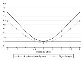
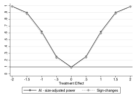
Figure 1.C: $N_{1}=25$	Figure 1.D: $N_{1}=50$

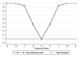
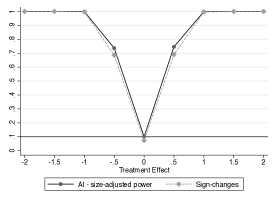
Notes: These figures present size-adjusted power for the asymptotic test based on AI at the 10%-level, and the power for the sign-changes test. We consider the setting presented in Panel A of Table 2, with $M=4$. In these simulations, $X|(W=w)\sim N(0,1)$ for $w\in\{0,1\}$, $Y(0)|(X=x,W=0)\sim N(0,1)$ for all $x\in\mathbb{R}$, $\mu_{1}(x)=\tau+x$, $(Y(1)-\mu_{1}(x))|(X=x,W=1)\sim N(0,1)$ for all $x\in\mathbb{R}$, and $N_{0}=1000$. For each combination of $N_{1}$ and $\tau$, we run 5000 simulations.

Table 3: Empirical illustration

	Rio de Janeiro				Sao Paulo
	$M=1$	$M=4$	$M=10$		$M=1$	$M=4$	$M=10$
	(1)	(2)	(3)		(4)	(5)	(6)
Treatment effects in 2010
Point Estimate	0.087	-0.003	0.046		0.000	0.018	0.004
p-values:
AI	0.091	0.941	0.086		0.995	0.601	0.924
RI-sign changes	0.123	0.938	0.179		0.996	0.609	0.917
Treatment effects in 2011
Point Estimate	0.043	-0.032	0.000		-0.019	-0.027	-0.013
p-values:
AI	0.566	0.396	0.997		0.746	0.475	0.692
RI-sign changes	0.662	0.438	0.997		0.734	0.496	0.693
Treatment effects in 2012
Point Estimate	0.070	-0.019	0.006		-0.072	-0.034	-0.019
p-values:
AI	0.263	0.522	0.885		0.169	0.383	0.616
RI-sign changes	0.306	0.576	0.896		0.185	0.382	0.495

Note: This table presents non-experimental results using a matching estimator with experimental control schools as treated observations and non-experimental schools as control observations. Columns 1 to 3 present results for Rio de Janeiro using 1, 4, or 10 nearest neighbors in the estimation, while columns 4 to 6 present results for Sao Paulo. We present the estimated effects separately for 2010, 2011, and 2012. For each estimate, we present p-values calculated based on the asymptotic distribution derived by AI, and based on the sign-changes test described in Section 4.

References

- Abadie et al., (2010) Abadie, A., Diamond, A., and Hainmueller, J. (2010). Synthetic Control Methods for Comparative Case Studies: Estimating the Effect of California’s Tobacco Control Program. Journal of the American Statiscal Association, 105(490):493–505.
- Abadie and Imbens, (2006) Abadie, A. and Imbens, G. W. (2006). Large sample properties of matching estimators for average treatment effects. Econometrica, 74(1):235–267.
- Abadie and Imbens, (2011) Abadie, A. and Imbens, G. W. (2011). Bias-corrected matching estimators for average treatment effects. Journal of Business & Economic Statistics, 29(1):1–11.
- Abadie and Imbens, (2012) Abadie, A. and Imbens, G. W. (2012). A martingale representation for matching estimators. Journal of the American Statistical Association, 107(498):833–843.
- Abadie and L’Hour, (2019) Abadie, A. and L’Hour, J. (2019). A penalized synthetic control estimator for disaggregated data.
- Armstrong and Kolesár, (2021) Armstrong, T. B. and Kolesár, M. (2021). Finite-sample optimal estimation and inference on average treatment effects under unconfoundedness.
- Barros et al., (2012) Barros, R., de Carvalho, M., Franco, S., and Rosalém, A. (2012). Impacto do projeto jovem de futuro. Estudos em Avaliação Educacional, 23(51):214–226.
- Bodory et al., (2018) Bodory, H., Camponovo, L., Huber, M., and Lechner, M. (2018). The finite sample performance of inference methods for propensity score matching and weighting estimators. Journal of Business & Economic Statistics, 0(ja):1–43.
- Botosaru and Ferman, (2019) Botosaru, I. and Ferman, B. (2019). On the role of covariates in the synthetic control method. Econometrics Journal, 22(2):117–130.
- Busso et al., (2014) Busso, M., DiNardo, J., and McCrary, J. (2014). New Evidence on the Finite Sample Properties of Propensity Score Reweighting and Matching Estimators. The Review of Economics and Statistics, 96(5):885–897.
- Cai et al., (2021) Cai, Y., Canay, I. A., Kim, D., and Shaikh, A. M. (2021). A user’s guide to approximate randomization tests with a small number of clusters.
- Canay and Kamat, (2017) Canay, I. A. and Kamat, V. (2017). Approximate Permutation Tests and Induced Order Statistics in the Regression Discontinuity Design. The Review of Economic Studies, 85(3):1577–1608.
- Canay et al., (2017) Canay, I. A., Romano, J. P., and Shaikh, A. M. (2017). Randomization tests under an approximate symmetry assumption. Econometrica, 85(3):1013–1030.
- Chernozhukov et al., (2017) Chernozhukov, V., Wuthrich, K., and Zhu, Y. (2017). An exact and robust conformal inference method for counterfactual and synthetic controls.
- Conley and Taber, (2011) Conley, T. G. and Taber, C. R. (2011). Inference with Difference in Differences with a Small Number of Policy Changes. The Review of Economics and Statistics, 93(1):113–125.
- Dehejia and Wahba, (1999) Dehejia, R. H. and Wahba, S. (1999). Causal effects in nonexperimental studies: Reevaluating the evaluation of training programs. Journal of the American Statistical Association, 94(448):1053–1062.
- Dehejia and Wahba, (2002) Dehejia, R. H. and Wahba, S. (2002). Propensity Score-Matching Methods For Nonexperimental Causal Studies. The Review of Economics and Statistics, 84(1):151–161.
- Doudchenko and Imbens, (2016) Doudchenko, N. and Imbens, G. (2016). Balancing, regression, difference-in-differences and synthetic control methods: A synthesis.
- Ferman, (2019) Ferman, B. (2019). On the Properties of the Synthetic Control Estimator with Many Periods and Many Controls. arXiv e-prints, page arXiv:1906.06665.
- Ferman and Pinto, (2017) Ferman, B. and Pinto, C. (2017). Placebo Tests for Synthetic Controls. MPRA Paper 78079, University Library of Munich, Germany.
- (21) Ferman, B. and Pinto, C. (2019a). Inference in differences-in-differences with few treated groups and heteroskedasticity. The Review of Economics and Statistics, 101(3):452–467.
- (22) Ferman, B. and Pinto, C. (2019b). Synthetic controls with imperfect pre-treatment fit.
- Ferman and Ponczek, (2017) Ferman, B. and Ponczek, V. (2017). Should we drop covariate cells with attrition problems? Mpra paper, University Library of Munich, Germany.
- Firpo and Possebom, (2018) Firpo, S. P. and Possebom, V. A. (2018). Synthetic control method: Inference, sensitivity analysis and confidence sets. Journal of Causal Inference, 6.
- Frolich, (2004) Frolich, M. (2004). Finite-sample properties of propensity-score matching and weighting estimators. The Review of Economics and Statistics, 86(1):77–90.
- Hahn and Shi, (2017) Hahn, J. and Shi, R. (2017). Synthetic control and inference. Econometrics, 5(4).
- Heckman et al., (1998) Heckman, J., Ichimura, H., Smith, J., and Todd, P. (1998). Characterizing selection bias using experimental data. Econometrica, 66(5):1017–1098.
- Heckman et al., (1996) Heckman, J. J., Ichimura, H., Smith, J., and Todd, P. (1996). Sources of selection bias in evaluating social programs: An interpretation of conventional measures and evidence on the effectiveness of matching as a program evaluation method. Proceedings of the National Academy of Sciences, 93(23):13416–13420.
- Heckman et al., (1997) Heckman, J. J., Ichimura, H., and Todd, P. E. (1997). Matching as an econometric evaluation estimator: Evidence from evaluating a job training programme. The Review of Economic Studies, 64(4):605–654.
- Hong et al., (2019) Hong, H., Leung, M. P., and Li, J. (2019). Inference on finite-population treatment effects under limited overlap. The Econometrics Journal, 23(1):32–47.
- Huber et al., (2013) Huber, M., Lechner, M., and Wunsch, C. (2013). The performance of estimators based on the propensity score. Journal of Econometrics, 175(1):1 – 21.
- Imbens, (2004) Imbens, G. (2004). Nonparametric estimation of average treatment effects under exogeneity: A review. Review of Economics and Statistics.
- Imbens, (2014) Imbens, G. (2014). Matching Methods in Practice: Three Examples. NBER Working Papers 19959, National Bureau of Economic Research, Inc.
- Imbens and Wooldridge, (2009) Imbens, G. and Wooldridge, J. (2009). Recent developments in the econometrics of program evaluation. Journal of Economic Literature, 47(1):5–86.
- Imbens and Rubin, (2015) Imbens, G. W. and Rubin, D. B. (2015). Causal Inference for Statistics, Social, and Biomedical Sciences: An Introduction. Cambridge University Press, New York, NY, USA.
- Khan and Tamer, (2010) Khan, S. and Tamer, E. (2010). Irregular identification, support conditions, and inverse weight estimation. Econometrica, 78(6):2021–2042.
- LaLonde, (1986) LaLonde, R. (1986). Evaluating the econometric evaluations of training programs with experimental data. American Economic Review, 76(4):604–20.
- Otsu and Rai, (2017) Otsu, T. and Rai, Y. (2017). Bootstrap inference of matching estimators for average treatment effects. Journal of the American Statistical Association, 112(520):1720–1732.
- Rosa, (2015) Rosa, L. (2015). Avaliação de impacto do programa jovem de futuro.
- Rosenbaum, (1984) Rosenbaum, P. R. (1984). Conditional permutation tests and the propensity score in observational studies. Journal of the American Statistical Association, 79(387):565–574.
- Rosenbaum, (2002) Rosenbaum, P. R. (2002). Covariance adjustment in randomized experiments and observational studies. Statist. Sci., 17(3):286–327.
- Rothe, (2017) Rothe, C. (2017). Robust confidence intervals for average treatment effects under limited overlap. Econometrica, 85(2):645–660.
- Rubin, (1973) Rubin, D. B. (1973). Matching to remove bias in observational studies. Biometrics, 29(1):159–183.
- Smith and Todd, (2001) Smith, J. A. and Todd, P. E. (2001). Reconciling conflicting evidence on the performance of propensity-score matching methods. The American Economic Review, 91(2):112–118.
- Smith and Todd, (2005) Smith, J. A. and Todd, P. E. (2005). Does matching overcome Lalonde’s critique of nonexperimental estimators? Journal of Econometrics, 125(1):305 – 353.