Orientational Memory of Active Particles in Multistate Non-Markovian Processes

Abstract

The orientational memory of particles can serve as an effective measure of diffusivity, spreading, and search efficiency in complex stochastic processes. We develop a theoretical framework to describe the decay of directional correlations in a generic class of stochastic active processes consisting of distinct states of motion characterized by their persistence and switching probabilities between the states. For exponentially distributed sojourn times, the orientation autocorrelation is analytically derived and the characteristic times of its crossovers are obtained in terms of the persistence of each state and the switching probabilities. We show how non-exponential sojourn-time distributions of interest, such as Gaussian and power-law distributions, can result from history-dependent transitions between the states. The relaxation behavior of the correlation function in such non-Markovian processes is governed by the history-dependence of the switching probabilities and cannot be solely determined by the mean sojourn times of the states.

Transport processes with distinct states of motion are ubiquitous in nature. Examples range from simple combinations of passive motility modes— as e.g. in chromatography or transport in amorphous materials— to more general mixtures of active and passive dynamics as frequently observed in living systems. Active dynamics of many biological agents consists of more than one motility mode. Migrating cells Chabaud et al. (2015); d’Alessandro et al. (2017), swimming bacteria Berg (2004); Najafi et al. (2018), molecular motors along cytoskeletal filaments Klumpp and Lipowsky (2005), and DNA-binding proteins Bauer and Metzler (2012); Meroz et al. (2009) are examples of agents that experience frequent transitions between two states of motion. While a full mathematical description of such multistate processes is challenging in general, a useful concept to describe the particle dynamics is the orientational memory, reflected e.g. in the velocity autocorrelations Peruani and Morelli (2007). The orientational correlation carries vital information about the diffusivity of the particle which affects its taxis, search, and transport efficiency Bartumeus and Levin (2008); Bénichou et al. (2011); Wadhams and Armitage (2004).

In order to handle multistate dynamics problems, the states are often approximated as simple stochastic processes, e.g. normal diffusion or ballistic motion, due to difficulties in analytical treatment of the full process. Although such simple mixtures have been broadly employed and succeeded in capturing some of the specific features of these systems Bressloff and Newby (2013); Shaebani and Rieger (2019); Taktikos et al. (2013); Jose et al. (2018); Pinkoviezky and Gov (2013); Theves et al. (2013); Shaebani et al. (2018); Watari and Larson (2010); Miyaguchi et al. (2019); Shaebani et al. (2016), they are generally inadequate to accurately describe the dynamics of a combination of active states with arbitrary persistencies. For instance, the run-and-tumble dynamics of bacteria is often modeled by ballistic runs and diffusion periods or random reorientation events Thiel et al. (2012); Angelani et al. (2009); Elgeti and Gompper (2015). However, partial disruption of flagellar bundles in the tumble state results in an active swimming with a weak persistence rather than a pure diffusive dynamics Najafi et al. (2018); Turner et al. (2016). Moreover, ballistic motion in the run state is a very rough assumption since the run trajectories can be extremely curved and the persistence, speed, and duration of the run state vary in response to environmental conditions and bacterial structure Berg (2004); Najafi et al. (2018); Patteson et al. (2015). Thus, a full description of the bacterial dynamics requires a technically challenging combination of two processes with arbitrary self-propulsions Detcheverry (2017).

The stochastic transitions between the states are often supposed to occur with constant probabilities, which leads to exponential sojourn-time distributions (as observed e.g. for the run-and-tumble dynamics of E. coli Taute et al. (2015); Molaei et al. (2014)). However, there is growing interest in non-exponential sojourn-time distributions. For instance, the run time of swarming bacteria Ariel et al. (2015) or the switching time of the rotation direction of flagellar motors Korobkova et al. (2004, 2006) follow power-law distributions. These observations evidence age-dependent transitions between the states d’Alessandro et al. (2017); Liu et al. (2018); Fedotov and Korabel (2017), which call for a detailed study of the effects of the history dependence of switching probabilities on sojourn-time distributions and particle dynamics. To design optimal navigation and taxis in non-Markovian active processes, a quantitative understanding of the influence of such memory effects on the orientational correlations is still lacking.

Here we develop a theoretical framework to quantify the orientational memory in multistate stochastic processes. Our approach allows us to calculate the orientational correlation function for arbitrary combinations of active and/or passive states and identify the timescales for crossovers of the correlation function. We verify how the exponential decay of correlations in processes with constant switching probabilities between the states depends on the persistence of the individual states and the switching probabilities. Moreover, we introduce specific history-dependent switching probabilities that lead to non-exponential sojourn-time distributions of interest, namely Gaussian and power-law forms. Our numerical results show that the tail behavior of the correlation function deviates from the exponential behavior; the temporal scale of the orientational memory changes in these non-Markovian processes with history-dependent transitions between the states.

First, we describe the stochastic discrete process that we use to model the active dynamics. The process consists of $n$ distinct states of motility, each characterized by the probability distributions $h_{{}_{\text{i}}}{\!(v)}$ and $f\!_{{}_{\text{i}}}{\!(\theta)}$ for the local speed $v$ and the directional change $\theta$ between successive steps of the random walk, respectively ($\text{i}{\in}\{1,{...},n\}$). We quantify the tendency to preserve the current direction of motion with a generalized self-propulsion parameter $p_{{}_{\text{i}}}{=}\!\int_{-{\pi}}^{{\pi}}\!\text{d}\theta\,e^{i\theta}f\!_{{}_{\text{i}}}{\!(\theta)}$. For a turning-angle distribution $f(\theta)$ which is symmetric with respect to the arrival direction (e.g. walking with left-right symmetry in 2D), the self-propulsion reduces to $p\,{=}\,\langle\cos\theta\rangle$, i.e. a real number within $[-1,1]$. However, for the general case of an asymmetric $f(\theta)$, $p$ has a nonzero imaginary part as well, leading to spiral trajectories Sadjadi et al. (2015). $p$ is related to the anomalous exponent $\beta$ (describing the time evolution of the MSD) via $\beta\,{=}\,1{+}\ln(1{+}p){/}\ln\,2$ Shaebani et al. (2014); thus, the value of $p$ reflects the diffusive regime of the particle dynamics: For a persistent random walk, $f(\theta)$ is peaked around $\theta{=}0$ (i.e. near forward directions) leading to a positive $p$ ($0{<}p{<}1$) and an anomalous exponent $\beta{>}1$ (superdiffusive dynamics). In the extreme case of a ballistic motion, one obtains $p{=}1$ and $\beta{=}2$. In contrast, $f(\theta)$ in an anti-persistent random walk is peaked around $\theta{=}\pi$ (i.e. near backward directions); thus, $p$ is negative (${-1}{<}p{<}0$) and $\beta{<}1$ (subdiffusive dynamics). A pure localization happens when the walker hopes back and forth forever, which leads to $p{=}{-1}$ and $\beta{=}0$. In case of normal diffusion, $f(\theta){=}\frac{1}{2\pi}$ is isotropic which results in $p{=}0$ and $\beta{=}1$. Stochastic transitions between the states occur with asymmetric probabilities $q_{{}_{\text{i}\rightarrow\text{j}}}$. When a switching occurs, the walker instantly adopts the distributions $h_{{}_{\text{i}}}{\!(v)}$ and $f\!_{{}_{\text{i}}}{\!(\theta)}$ of the new state.

We consider an active motion in 2D in the following for brevity (extension to 3D is straightforward; see e.g. the treatment of a single-state persistent random walk in Sadjadi et al. (2015)). As shown in the schematic Fig. 1, the orientation of the walker at successive time steps $t{-}\Delta t$ and $t$ is denoted with angles $\phi$ and $\gamma$, respectively, and the directional change $\theta$ during these two steps is given by $\theta{=}\gamma{-}\phi$. By introducing the orientation unit vectors $\hat{\bm{u}}_{t{-}\Delta t}\,{=}\!\left[\!\!\begin{array}[]{ccccccccc}\cos\phi\\ \sin\phi\end{array}\!\!\right]$ and $\hat{\bm{u}}_{t}\,{=}\!\left[\!\!\begin{array}[]{ccccccccc}\cos\gamma\\ \sin\gamma\end{array}\!\!\right]$ and the probability density functions $S_{{{}_{t{-}\Delta t}},{{}_{\text{i}}}}\!(\phi)$ and $S_{{{}_{t}},{{}_{\text{i}}}}\!(\gamma)$ to find the walker in state i with the given orientation, the orientational state of the system at successive time steps $t{-}\Delta t$ and $t$ can be represented as ${\bf S}_{t{-}\Delta t}{=}\!\left(\!\!\begin{array}[]{ccccccccc}S_{{{}_{t{-}\Delta t}},{{}_{\text{1}}}}\!(\phi)\\ \vdots\\ S_{{{}_{t{-}\Delta t}},{{}_{\text{n}}}}\!(\phi)\end{array}\!\!\right)$ and ${\bf S}_{t}{=}\!\left(\!\!\begin{array}[]{ccccccccc}S_{{{}_{t}},{{}_{\text{1}}}}\!(\gamma)\\ \vdots\\ S_{{{}_{t}},{{}_{\text{n}}}}\!(\gamma)\end{array}\!\!\right)$. The following set of master equations describe the temporal evolution of the stochastic process

$${\bf S}_{t}={\bf M}\;{\bf S}_{t{-}\Delta t},$$ (1)

with $\bf M$ being the transition matrix given by

$${\bf M}{=}\!\!\!\displaystyle\int_{\!{-}\pi}^{\pi}\!\!\!\!\!\!d\phi\!\!\displaystyle\left[\!\!\begin{array}[]{cccc}(1{-}\!\!\!\sum\limits_{j{\neq}1}\!\!q_{{}_{\text{1}\rightarrow\text{j}}}\!)f\!_{{}_{\text{1}}}{\!(\theta)}&\!\!q_{{}_{\text{2}\rightarrow\text{1}}}f\!_{{}_{\text{1}}}{\!(\theta)}&\!\!\cdots&\!\!q_{{}_{\text{n}\rightarrow\text{1}}}f\!_{{}_{\text{1}}}{\!(\theta)}\\ \vdots&\!\!\ddots&&\!\!\vdots\\ \!\!\!\!\!\!\!\!q_{{}_{\text{1}\rightarrow\text{n}}}f\!_{{}_{\text{n}}}{\!(\theta)}&\!\!\!q_{{}_{\text{2}\rightarrow\text{n}}}f\!_{{}_{\text{n}}}{\!(\theta)}&\!\!\!\!\!\cdots&\!\!\!\!\!(1{-}\!\!\!\!\sum\limits_{j{\neq}n}\!\!q_{{}_{\text{n}\rightarrow\text{j}}}\!)f\!_{{}_{\text{n}}}{\!(\theta)}\end{array}\!\!\!\right]\!\!\!.\!\!\;\;\;\;\;\;$$ (5)

An off-diagonal element $M_{ij}$ represents the possibility of switching from state $j$ to $i$ with probability $q_{{}_{\text{j}\rightarrow\text{i}}}$ while the diagonal element $M_{ii}$ takes into account the possibility of remaining in state $i$ with probability $1{-}\!\!\sum\limits_{j{\neq}i}\!\!q_{{}_{\text{i}\rightarrow\text{j}}}$. The orientational change $\theta$ from any arbitrary direction $\phi$ to the new direction $\gamma$ is deduced from the turning-angle distribution $f\!_{{}_{\text{i}}}{\!(\theta)}$ via the integral $\int_{\!{-}\pi}^{\pi}d\phi\,f\!_{{}_{\text{i}}}{\!(\gamma{-}\phi)}$ over all possibilities of $\phi$. In case of a two-state process the transition matrix reduces to

$${\bf M}{=}\!\!\displaystyle\int_{\!{-}\pi}^{\pi}\!\!\!\!d\phi\displaystyle\left[\!\!\begin{array}[]{cc}(1{-}q_{{}_{\text{I}\rightarrow\text{I\!I}}}\!)f\!_{{}_{\text{I}}}{\!(\theta)}&\!\!q_{{}_{\text{I\!I}\rightarrow\text{I}}}\,f\!_{{}_{\text{I}}}{\!(\theta)}\\ \!\!\!\!\!\!\!\!q_{{}_{\text{I}\rightarrow\text{I\!I}}}\,f\!_{{}_{\text{I\!I}}}{\!(\theta)}&(1{-}q_{{}_{\text{I\!I}\rightarrow\text{I}}}\!)f\!_{{}_{\text{I\!I}}}{\!(\theta)}\end{array}\!\!\right]\!\!.\!\!\;\;\;\;\;\;$$ (8)

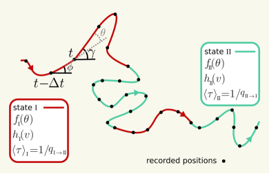
Figure 1: A sample trajectory of the persistent random walker with two states of motion. Each state is characterized by its turning-angle distribution $f\!_{{}_{\text{i}}}{\!(\theta)}$, speed distribution $h_{{}_{\text{i}}}{\!(v)}$, and mean sojourn time $\langle\tau\rangle_{{}_{\text{i}}}$.

Constant switching probabilities.— The transitions between the states with constant probabilities $q_{{}_{\text{i}\rightarrow\text{j}}}$ lead to exponential distributions $P\!_{{}_{\text{i}}}(\tau)\,{\sim}\,\text{exp}\big{[}\ln(1{-}\!\!\sum\limits_{j{\neq}i}\!q_{{}_{\text{i}\rightarrow\text{j}}}\!)\;\!\tau\big{]}$ for the sojourn time $\tau$ in each state with the mean sojourn times $\langle\tau\rangle_{{}_{\text{i}}}{=}1{/}\!\sum\limits_{j{\neq}i}\!q_{{}_{\text{i}\rightarrow\text{j}}}$. For constant switching probabilities, we solve Eqs. (1) in Fourier space, which enables us to calculate the orientational correlations. While the formalism is developed for multi-state processes in general, hereafter we consider a two-state dynamics, as the most frequent multi-state process in natural systems (Fig. 1). Using the Fourier transform $S_{{{}_{t}},{{}_{\text{i}}}}\!(m){=}\!\int_{-{\pi}}^{{\pi}}\!\text{d}\gamma\,e^{im\gamma}S_{{{}_{t}},{{}_{\text{i}}}}\!(\gamma)$, the master equations (1) lead to

$$\!\!\!{\bf S}_{t}(m) ={\bf\widetilde{M}}\;{\bf S}_{t{-}\Delta t}(m)$$

$$\equiv\!\displaystyle\left[\!\!\begin{array}[]{cc}(1{-}q_{{}_{\text{I}\rightarrow\text{I\!I}}})f\!_{{}_{\text{I}}}(m)&q_{{}_{\text{I\!I}\rightarrow\text{I}}}\,f\!_{{}_{\text{I}}}(m)\\ q_{{}_{\text{I}\rightarrow\text{I\!I}}}\,f\!_{{}_{\text{I\!I}}}(m)&(1{-}q_{{}_{\text{I\!I}\rightarrow\text{I}}})f\!_{{}_{\text{I\!I}}}(m)\end{array}\!\!\!\right]\!{\bf S}_{t{-}\Delta t}(m),$$ (11)

with ${\bf S}_{t{-}\Delta t}(m){=}\!\left(\!\!\begin{array}[]{cc}S_{{{}_{t{-}\Delta t}},{{}_{\text{I}}}}\!(m)\\ S_{{{}_{t{-}\Delta t}},{{}_{\text{I\!I}}}}\!(m)\end{array}\!\!\right)$, ${\bf S}_{t}(m){=}\!\left(\!\!\begin{array}[]{cc}S_{{{}_{t}},{{}_{\text{I}}}}\!(m)\\ S_{{{}_{t}},{{}_{\text{I\!I}}}}\!(m)\end{array}\!\!\right)$, and $f\!_{{}_{\text{i}}}(m)$ being the Fourier transform of $f\!_{{}_{\text{i}}}(\theta)$. Equation (11) can be recursively solved to obtain ${\bf S}_{t}(m)\,{=}\,{\bf\widetilde{M}}^{{}^{t}}{\bf S}_{0}(m)$. Alternatively, a combined Fourier-z-transform approach Sadjadi et al. (2008) can be followed to reach the same result.

The orientational correlation function after time $t$ can be calculated as

$$\!\!\!\!\!\!\!\!\!\!\!\!\!\!\!\!\!\!\!\!\!\!\!\!\!\!\!\langle\hat{\bm{u}}_{t}{\cdot}\hat{\bm{u}}_{0}\rangle =\langle\cos(\gamma_{{}_{t}}{-}\gamma_{{}_{0}})\rangle$$

$$=\!\int_{-{\pi}}^{{\pi}}\!\!\!\!\!\text{d}\gamma\int_{-{\pi}}^{{\pi}}\!\!\!\!\!\text{d}\gamma^{\prime}\,\cos(\gamma{-}\gamma^{\prime})\,S(\gamma,t;\gamma^{\prime},0),\,\,\,\,\,\,\,\,\,\,\,$$ (12)

where $S(\gamma,t;\gamma^{\prime},0)$ is the joint probability distribution of having the orientation $\gamma$ and $\gamma^{\prime}$ at time $t$ and $0$, respectively. Assuming an initial state $S_{0}(\gamma^{\prime})\,{=}\,\delta(\gamma^{\prime}{-}\gamma_{{}_{0}})$, the joint probability can be written as

$$S(\gamma,t;\gamma^{\prime},0)=S(\gamma,t|\gamma^{\prime},0)\,\delta(\gamma^{\prime}{-}\gamma_{{}_{0}}).$$ (13)

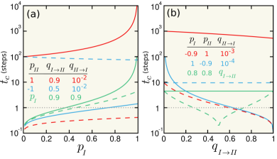
Figure 2: Characteristic time $t_{\text{c}}$ in terms of (a) $p_{{}_{\text{I}}}$ and (b) $q_{{}_{\text{I}\rightarrow\text{I\!I}}}$ for different values of other key parameters. The solid (dashed) lines represent $t_{\text{c}_{+}}$ ($t_{\text{c}_{-}}$) timescales. The dotted gray lines correspond to $t_{\text{c}}{=}1$, below which the particle practically carries no orientational memory.

​​We obtain, after some algebra, the following exact closed expression for the orientational correlation function

$$\langle\hat{\bm{u}}_{t}{\cdot}\hat{\bm{u}}_{0}\rangle=\Big{(}\frac{1}{2}{+}\frac{\mathcal{L}}{2\mathcal{H}}\Big{)}\text{e}^{-t{/}t_{\text{c}_{+}}}{+}\Big{(}\frac{1}{2}{-}\frac{\mathcal{L}}{2\mathcal{H}}\Big{)}\text{e}^{-t{/}t_{\text{c}_{-}}},$$ (14)

with $\mathcal{L}{=}\!\!\!\!\!\!\sum\limits_{\text{i}{\in}\{\text{I},\text{I\!I}\}}\!\!\!\!\!\!\big{[}(1{-}\lambda_{\text{i}}\!)(2S\!_{{}_{0,\text{i}}}\!\!{-}1\!){+}2S\!_{{}_{0,\text{i}}}q_{{}_{\text{i}\rightarrow\text{j}}}p_{{}_{\text{j}}}\big{]}\!$, $\!\mathcal{H}{=}\sqrt{\!(\lambda_{{}_{\text{I\!I}}}\!\!{-}\lambda_{{}_{\text{I}}}\!)^{2}{+}\mathcal{C}}$, $\mathcal{C}{=}\!\!\!\!\prod\limits_{\text{i}{\in}\{\text{I},\text{I\!I}\}}\!\!\!\!2q_{{}_{\text{i}\rightarrow\text{j}}}p_{{}_{\text{j}}}$, and $\lambda_{{}_{\text{i}}}{=}1{-}p_{{}_{\text{i}}}(1{-}q_{{}_{\text{i}\rightarrow\text{j}}}\!)$. The initial condition $S\!_{{}_{0,\text{i}}}$— i.e. the probability of initially starting in state i— influences the orientational correlation function through the prefactors of the exponential terms. In the following, we choose an initially equilibrated system with steady probabilities $S\!_{{}_{\text{I}}}^{\;\text{st}}{=}\frac{q_{{}_{\text{I\!I}\rightarrow\text{I}}}}{q_{{}_{\text{I}\rightarrow\text{I\!I}}}{+}q_{{}_{\text{I\!I}\rightarrow\text{I}}}}$ and $S\!_{{}_{\text{I\!I}}}^{\;\text{st}}{=}\frac{q_{{}_{\text{I}\rightarrow\text{I\!I}}}}{q_{{}_{\text{I}\rightarrow\text{I\!I}}}{+}q_{{}_{\text{I\!I}\rightarrow\text{I}}}}$. Note that starting from an arbitrary $S\!_{{}_{0,\text{i}}}$, the Markov process of switching between the two states exponentially approaches the steady state with the relaxation time $t{=-1}{/}\ln|1{-}q_{{}_{\text{I}\rightarrow\text{I\!I}}}{-}q_{{}_{\text{I\!I}\rightarrow\text{I}}}|$ Hafner et al. (2016). Nevertheless, the characteristic times $t_{\text{c}_{\pm}}$ in Eq. (14) are independent of the initial conditions and given by

$$t_{\text{c}_{\pm}}{=}{-1}\Big{/}\ln\Big{|}\frac{\mathcal{A}{\pm}\sqrt{\mathcal{A}^{2}{-}4p_{{}_{\text{I}}}p_{{}_{\text{I\!I}}}(1{-}q_{{}_{\text{I}\rightarrow\text{I\!I}}}{-}q_{{}_{\text{I\!I}\rightarrow\text{I}}})}}{2}\Big{|},$$ (15)

with $\mathcal{A}\,{=}\!\!\!\!\!\sum\limits_{\text{i}{\in}\{\text{I},\text{I\!I}\}}\!\!\!\!\!p_{{}_{\text{i}}}(1{-}q_{{}_{\text{i}\rightarrow\text{j}}})$. The temporal scale of orientational correlations, set by $t_{\text{c}_{\pm}}$, can vary by several orders of magnitude by changing the self-propulsions $p_{{}_{\text{i}}}$ and switching probabilities $q_{{}_{\text{i}\rightarrow\text{j}}}$, as shown in Fig. 2.

Equation (14) implies that constant transition probabilities lead to an exponential decay of the orientational memory of the walker; as a result, the trajectory eventually gets randomized after a crossover time controlled by the longest characteristic time. The shape of the correlation profiles strongly depends on the choice of $p_{{}_{\text{i}}}$ and $q_{{}_{\text{i}\rightarrow\text{j}}}$ parameters; see Fig. 3. If the timescales $t_{\text{c}_{+}}$ and $t_{\text{c}_{-}}$ are well separated, the correlation function possesses two inflection points. For comparison of the characteristic timescales, $\mathcal{O}(t_{\text{c}_{+}}{/}t_{\text{c}_{-}}){\sim}10\;(10^{3})$ for the purple (red) curve in Fig. 3. An oscillatory dynamics emerges when at least one of the states of motion is strongly sub-diffusive, i.e. has a large negative value of $p_{i}$. The particle dynamics in such a state is strongly antipersistent and the particle hopes frequently back and forth without a significant net motion. Since the direction of motion is nearly reversed at every timestep, the orientational correlation between successive steps is weak while between every two steps is strong. Similar oscillations can be observed for other transport properties of interest such as the mean square displacement Tierno et al. (2012); Shaebani et al. (2014). In order to confirm the validity of the analytical predictions we perform extensive Monte Carlo simulations of the same stochastic process: A random walker in 2D with two different modes of self-propulsion is considered and the walker can spontaneously change the motility mode at each timestep according to given asymmetric switching probabilities. The simulation results presented in Fig. 3 are averaged over an ensemble of $10^{5}$ realizations. The analytical predictions are in perfect agreement with the simulation results.

Equation (14) reduces to $\text{e}^{-t{/}t_{\text{c}}}$ with $t_{\text{c}}{=-}1{/}\ln p$ for a single-state active motion with self-propulsion $p$ Tierno and Shaebani (2016). Another example is the exponential decay of correlations in a run-and-tumble process— consisting of successive periods of ballistic run ($p_{{}_{\text{r}}}{=}1$) and pure diffusion ($p_{{}_{\text{t}}}{=}0$)—, with a characteristic time which is purely governed by the run-to-tumble switching probability $q_{{}_{\text{r}\rightarrow\text{t}}}$ as $t_{\text{c}}{=}\frac{-1}{\ln(1{-}q_{{}_{\text{r}\rightarrow\text{t}}})}$. More generally, Eq. (14) enables one to calculate the orientational correlation function for an arbitrary combination of two anomalous diffusive dynamics. Assuming an uncorrelated speed and directional persistence, the velocity autocorrelation can be deduced as $\langle{\bm{v}}_{t}{\cdot}{\bm{v}}_{0}\rangle\,{=}\,\langle v\rangle\!^{{}^{2}}\langle\hat{\bm{u}}_{t}{\cdot}\hat{\bm{u}}_{0}\rangle$, where $\langle v\rangle\,{=}\,S\!_{{}_{\text{I}}}^{\;\text{st}}\langle v\rangle_{{}_{\text{I}}}{+}S\!_{{}_{\text{I\!I}}}^{\;\text{st}}\langle v\rangle_{{}_{\text{I\!I}}}$; however, one should take into account persistence-speed correlations in general Maiuri et al. (2015); Jerison and Quake (2020); Shaebani et al. (2020); Wu et al. (2014). We also note that instead of the correlation timescale one can alternatively represent the formalism in terms of the correlation length scale, using the local persistence length $\ell_{p}$ extracted from $\cos(\theta){=}\text{e}^{v\Delta t{/}\ell_{p}}$ Landau and Lifshitz (1958); Doi and Edwards (1986).

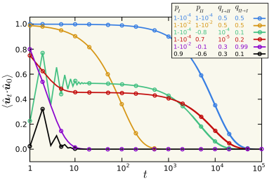
Figure 3: Orientational correlation function as a function of time for different values of the key parameters of the model. The symbols denote simulation results and the solid lines correspond to analytical predictions via Eq. (14).

Age-dependent switching probabilities.— Next we consider non-Markovian stochastic processes with age-dependent transition probabilities $q_{{}_{\text{i}\rightarrow\text{j}}}(\tau)$ between the states, which result in non-exponential sojourn time distributions $P\!_{{}_{\text{i}}}(\tau)$ in general. In this class of stochastic processes, the probability of switching from state i to j at each timestep (and thus the probability of remaining in state i) depends on the current residence time $\tau$ in state i. Therefore, we obtain the probability of a sojourn time $\tau$ in each state as $P\!_{{}_{\text{i}}}(\tau)\!=\!\frac{1}{\mathcal{N}}\!\prod\limits_{t{=}1}^{\tau{-}1}\!\!\big{(}1{-}q_{{}_{\text{i}\rightarrow\text{j}}}(t)\big{)}$, with the normalization factor $\mathcal{N}\,{=}\,1{+}\sum\limits_{t^{\prime}{=}1}^{\tau{-}1}\prod\limits_{t{=}1}^{t^{\prime}}\!\!\big{(}1{-}q_{{}_{\text{i}\rightarrow\text{j}}}(t)\big{)}$. Here we introduce two types of memory kernels which enhance or reduce the duration of stay at each state and modify $P\!_{{}_{\text{i}}}(\tau)$ towards known non-exponential forms, namely power-law and Gaussian distributions. The first example is an inverse dependence of the switching probability on the age $\tau$ of the state Fedotov and Korabel (2017). We assign a maximal probability $q^{\circ}_{{}_{\text{i}{\rightarrow}\text{j}}}$ to switch from state i to another state j if the walker has just switched to state i in the previous timestep. However, if the walker remains in state i for a longer time, the switching probability to state j decreases over time according to an age-dependent form

$$q_{{}_{\text{i}\rightarrow\text{j}}}(\tau)\,{=}\,\displaystyle\frac{q^{\circ}_{{}_{\text{i}{\rightarrow}\text{j}}}}{\tau^{\alpha}}.$$ (16)

We tune the history dependence via the exponent $0\,{\leq}\,\alpha\,{\leq}\,1$. A larger $\alpha$ leads to a faster decay of the switching probability $q_{{}_{\text{i}\rightarrow\text{j}}}$, i.e., a longer stay in state i. While $\alpha{=}0$ corresponds to a constant switching probability and an exponential sojourn time distribution $P\!_{{}_{\text{i}}}(\tau)$, the limit $\alpha{=}1$ results in $P\!_{{}_{\text{i}}}(\tau)\,{\propto}\,\frac{\Gamma(\tau{-}q^{\circ}_{{}_{\text{i}{\rightarrow}\text{j}}})}{\Gamma(\tau)}$ with $\Gamma(n){=}(n{-}1)!$ being the gamma function. The tail of the sojourn time distribution decays as a power-law $P\!_{{}_{\text{i}}}(\tau)\,{\sim}\,\tau^{-q^{\circ}_{{}_{\text{i}{\rightarrow}\text{j}}}}$ for which the mean sojourn time $\langle\tau\rangle_{{}_{\text{i}}}$ diverges. The gradual change of $P\!_{{}_{\text{i}}}(\tau)$ and $\langle\tau\rangle_{{}_{\text{i}}}$ with increasing $\alpha$ from $0$ to $1$, resulting from Eq. (16), is shown in Fig. 4(a),(b). There have been examples of power-law sojourn-time distributions in natural stochastic processes as, for example, for the run time of swarming bacteria or the switching time of the rotation direction of flagellar motors Ariel et al. (2015); Korobkova et al. (2004, 2006). Our second choice of the history dependence is an exponentially saturating switching probability with the age $\tau$ of state i as

$$q_{{}_{\text{i}\rightarrow\text{j}}}(\tau)\,{=}\,1-\big{(}1{-}q^{\circ}_{{}_{\text{i}{\rightarrow}\text{j}}}\big{)}\,\text{exp}\Big{[}-\frac{\tau{-}1}{\tau_{\text{c}}}\Big{]}.$$ (17)

Here, $\tau_{\text{c}}$ is the characteristic age and $q^{\circ}_{{}_{\text{i}{\rightarrow}\text{j}}}$ is the minimal switching probability from state i to j (which applies in case of a newly started state i). The switching probability to state j increases with further staying in state i. In the limit $\tau{\rightarrow}\infty$, $q_{{}_{\text{i}\rightarrow\text{j}}}(\tau)$ approaches $1$, i.e. a transition from state i to j becomes highly probable. It can be shown that a gradual increase of the switching probability according to Eq. (17) results in a Gaussian sojourn time distribution $P\!_{{}_{\text{i}}}(\tau)$; see Fig. 4(c). Note that straight lines in log-lin plots of $P\!_{{}_{\text{i}}}(\tau)$ vs $\tau^{2}$ represent a Gaussian decay. Figure 4(c) also shows that $P\!_{{}_{\text{i}}}(\tau)$ is broader at larger values of $\tau_{\text{c}}$. A possible realization for a Gaussian sojourn-time distribution can be a tactic motion where the changes of the states are prevented by the level of a chemical in the environment which decreases exponentially over time.

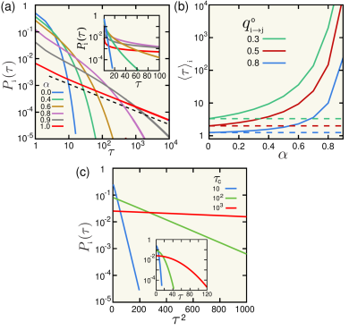
Figure 4: (a) Sojourn time distribution $P\!_{{}_{\text{i}}}(\tau)$ in log-log scale in a stochastic process with transition probabilities according to Eq. (16) for $q^{\circ}_{{}_{\text{i}{\rightarrow}\text{j}}}{=}0.5$. The dashed guide line indicates a power-law decay. Inset: Same plot in log-lin scale. (b) Mean sojourn time in state i vs $\alpha$. The dashed lines denote $\langle\tau\rangle_{{}_{\text{i}}}$ in the constant-switching process with the same $q^{\circ}_{{}_{\text{i}{\rightarrow}\text{j}}}$. (c) $P\!_{{}_{\text{i}}}(\tau)$ vs $\tau^{2}$ in a process described by Eq. (17) for $q^{\circ}_{{}_{\text{i}{\rightarrow}\text{j}}}{=}0$ and different values of $\tau_{\text{c}}$. Inset: $P\!_{{}_{\text{i}}}(\tau)$ vs $\tau$ in log-lin scale.

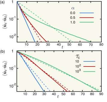
Figure 5: Comparison between the orientational correlations in processes with constant and history-dependent switching probabilities. The solid lines are $\langle\hat{\bm{u}}_{t}{\cdot}\hat{\bm{u}}_{0}\rangle$ for a history dependence in state I according to (a) Eq. (16) or (b) Eq. (17). A constant-switching process is considered for state II. The dashed lines represent the corresponding results for a constant-switching process in state I with the same mean sojourn time as in the history-dependent process. $p_{{}_{\text{I}}}\,{=}\,0.96$, $p_{{}_{\text{I\!I}}}\,{=}\,0.5$, $q^{\circ}_{{}_{\text{I}\rightarrow\text{I\!I}}}\,{=}\,q_{{}_{\text{I\!I}\rightarrow\text{I}}}\,{=}\,0.5$.

By introducing the probability density function $S_{{{}_{t}},{{}_{\text{i}}}}^{\tau}\!(\gamma)$ to find the walker in state i with age $\tau$ and orientation $\gamma$ at time $t$, the following master equations hold in the general case of age-dependent switching probabilities

$$\begin{cases}S_{{{}_{t}},{{}_{\text{i}}}}^{\tau}\!(\gamma)\,{=}\,\Big{(}1{-}q_{{}_{\text{i}\rightarrow\text{j}}}(\tau{-}1)\Big{)}\!\!\displaystyle\int\!\!d\phi\,f\!_{{}_{\text{i}}}(\gamma{-}\phi)\,S_{{{}_{t{-}1}},{{}_{\text{i}}}}^{\tau{-}1}\!(\phi),&\tau{>}1,\vspace{3mm}\\ S_{{{}_{t}},{{}_{\text{i}}}}^{1}\!(\gamma)\,{=}\displaystyle\sum\limits_{\tau^{\prime}{=}1}^{t{-}1}q_{{}_{\text{j}\rightarrow\text{i}}}(\tau^{\prime})\!\!\displaystyle\int\!\!d\phi\,f\!_{{}_{\text{i}}}(\gamma{-}\phi)\,S_{{{}_{t{-}1}},{{}_{\text{j}}}}^{\tau^{\prime}}\!(\phi),&\tau{=}1.\end{cases}$$ (18)

By recursively solving the Fourier transform of Eqs. (18) and combining them, we obtain

$$S_{{{}_{t}},{{}_{\text{i}}}}^{\tau}\!(m){=}f\!_{{}_{\text{i}}}^{{}^{\,\tau}}\!\!(m)\Bigg{[}\!\prod\limits_{\text{k}{=}1}^{\tau{-}1}\!\!\Big{(}1{-}q_{{}_{\text{i}\rightarrow\text{j}}}\!(\text{k})\Big{)}\!\Bigg{]}\sum\limits_{\tau^{\prime}{=}1}^{t{-}\tau}\!q_{{}_{\text{j}\rightarrow\text{i}}}(\tau^{\prime})S_{{{}_{t{-}\tau}},{{}_{\text{j}}}}^{\tau^{\prime}}\!(m).$$ (19)

To numerically obtain the orientational correlation function, we assume that the walker starts the motion with orientation $\gamma_{{}_{0}}$— i.e. an initial state $S\!_{{}_{0}}(m){=}e^{i\,m\,\gamma_{{}_{0}}}$— with an equal probability for being in each state. Using the Fourier transforms $f\!_{{}_{\text{I}}}\!(m)$ and $f\!_{{}_{\text{I\!I}}}\!(m)$ of the given turning-angle distributions, we perform Monte Carlo simulations with the desired forms for the age dependence of the switching probabilities between the states. By an ensemble of $10^{6}$ realizations of a chain of $t$ stochastic steps, we calculate $S_{{{}_{t}},{{}_{\text{i}}}}^{\tau}\!(m)$ and by the inverse Fourier transform extract the joint probability distribution of having the orientation $\gamma$ and $\gamma_{{}_{0}}$ at time $t$ and $0$, respectively. Then, following a similar procedure as described in Eqs. (12) and (13), we numerically obtain the correlation function $\langle\cos(\gamma_{{}_{t}}{-}\gamma_{{}_{0}})\rangle$.

The main characteristic of the orientational correlation function in processes with constant switching probabilities is the exponential relaxation according to Eq. (14). The behavior is governed by the switching probabilities (equivalently the mean sojourn times) as well as the persistence of the states. According to Eqs. (14) and (15), the long-term relaxation dynamics are dominated by the state with a higher persistence. To better understand the role of age dependence of the switching probabilities, we consider a two-state process with high and low persistencies and with constant $q_{{}_{\text{I\!I}\rightarrow\text{I}}}$ but history-dependent $q_{{}_{\text{I}\rightarrow\text{I\!I}}}$ transitions. Upon increasing $\alpha$ towards a power-law sojourn-time distribution in the high-persistence state I, the orientational correlation function deviates from the exponential behavior and the tail becomes broader, as shown in Fig. 5(a). Nevertheless, the decay is still faster than a power-law even at $\alpha\,{=}\,1$ (though it was recently reported that the relaxation behavior of the stochastic processes with power-law sojourn times may crossover at longer timescales Miyaguchi et al. (2019)). The non-exponential form of the correlation function evidences that the behavior is not controlled by the mean sojourn times of the states anymore. For comparison, we also plot the correlation in a constant-switching process with the same mean sojourn time as in the history-dependent process; the differences become more pronounced with increasing $\alpha$; see dashed lines in Fig. 5(a). In a process with Gaussian sojourn time distribution in state I, Fig. 5(b) shows that the correlation decays faster than exponential (yet slower than Gaussian) for all choices of the characteristic history relaxation $\tau_{\text{c}}$. Similarly to the power-law age-dependence case, the behavior is not solely governed by the mean sojourn times of the states [see dashed lines in Fig. 5(b)]; however, the differences with a constant-switching process becomes negligible for $\tau_{\text{c}}{\rightarrow}\infty$. In this section we linked simple non-exponential forms of sojourn-time distribution (namely power-law and normal distributions) to non-Markovian transitions between the states of motion. More generally, realistic sojourn-time distributions in multi-state natural processes (that do not necessarily follow well-defined mathematical forms) can be also originated from (and numerically linked to) age-dependent switching probabilities between the states. Such transitions may lead to stronger or weaker orientational correlations, depending on whether the age-dependent switching role encourages or discourages a longer stay in the states. While the orientational memory trivially depends on the self-propulsion of the active agent, our findings verify that the switching statistics between the states can also dramatically influence the orientational memory.

We analytically investigated the temporal evolution of orientational correlations in multistate active processes and derived an exact expression for the orientation autocorrelation in processes with constant switching probabilities between the states. Our theoretical approach opens up a new avenue to study a broad range of natural processes with distinct states of motility. For instance, the formalism can be generalized to consider stochastic dynamics with correlated persistence and speed as observed in cell migration Maiuri et al. (2015); Jerison and Quake (2020); Shaebani et al. (2020); Wu et al. (2014). It can be also extended to include the possibility of sharp directional changes during the switching events, motivated by the non-smooth tumble-to-run transitions commonly observed in bacterial dynamics Berg (2004); Najafi et al. (2018). Our results for age-dependent transitions between the states reveal that the orientational memory of the agent in such non-Markovian processes can be enhanced or suppressed depending on the introduced history dependence of the transitions. The approach is broadly applicable to other classes of non-Markovian stochastic processes with different functionalities for the age dependence of transition probabilities. The orientational memory of an active agent reflects its ability to efficiently explore the environment. Thus, our findings have far-reaching implications particularly for the design of optimal taxis, navigation, and search strategies in active systems.

We acknowledge support from the Deutsche Forschungsgemeinschaft (DFG) through the collaborative research center SFB 1027. MRS acknowledges support by Saarland University NanoBioMed initiative Grant No. 7410110401.

References

- Chabaud et al. (2015) M. Chabaud et al., Nat. Commun. 6, 7526 (2015).
- d’Alessandro et al. (2017) J. d’Alessandro, A. P. Solon, Y. Hayakawa, C. Anjard, F. Detcheverry, J.-P. Rieu, and C. Rivière, Nat. Phys. 13, 999 (2017).
- Berg (2004) H. C. Berg, E. coli in motion (Springer Verlag, New York, 2004).
- Najafi et al. (2018) J. Najafi, M. R. Shaebani, T. John, F. Altegoer, G. Bange, and C. Wagner, Science Adv. 4, eaar6425 (2018).
- Klumpp and Lipowsky (2005) S. Klumpp and R. Lipowsky, Phys. Rev. Lett. 95, 268102 (2005).
- Bauer and Metzler (2012) M. Bauer and R. Metzler, Biophy. J. 102, 2321 (2012).
- Meroz et al. (2009) Y. Meroz, I. Eliazar, and J. Klafter, J. Phys. A 42, 434012 (2009).
- Peruani and Morelli (2007) F. Peruani and L. G. Morelli, Phys. Rev. Lett. 99, 010602 (2007).
- Bartumeus and Levin (2008) F. Bartumeus and S. A. Levin, Proc. Natl. Acad. Sci. USA 105, 19072 (2008).
- Bénichou et al. (2011) O. Bénichou, C. Loverdo, M. Moreau, and R. Voituriez, Rev. Mod. Phys. 83, 81 (2011).
- Wadhams and Armitage (2004) G. H. Wadhams and J. P. Armitage, Nat. Rev. Mol. Cell Biol. 5, 1024 (2004).
- Bressloff and Newby (2013) P. C. Bressloff and J. M. Newby, Rev. Mod. Phys. 85, 135 (2013).
- Shaebani and Rieger (2019) M. R. Shaebani and H. Rieger, Front. Phys. 7, 120 (2019).
- Taktikos et al. (2013) J. Taktikos, H. Stark, and V. Zaburdaev, PLOS ONE 8, 1 (2013).
- Jose et al. (2018) R. Jose, L. Santen, and M. R. Shaebani, Biophys. J. 115, 2014 (2018).
- Pinkoviezky and Gov (2013) I. Pinkoviezky and N. S. Gov, Phys. Rev. E 88, 022714 (2013).
- Theves et al. (2013) M. Theves, J. Taktikos, V. Zaburdaev, H. Stark, and C. Beta, Biophys. J. 105, 1915 (2013).
- Shaebani et al. (2018) M. R. Shaebani, R. Jose, C. Sand, and L. Santen, Phys. Rev. E 98, 042315 (2018).
- Watari and Larson (2010) N. Watari and R. G. Larson, Biophys. J. 98, 12 (2010).
- Miyaguchi et al. (2019) T. Miyaguchi, T. Uneyama, and T. Akimoto, Phys. Rev. E 100, 012116 (2019).
- Shaebani et al. (2016) M. R. Shaebani, P. Aravind, O. Albrecht, and S. Ludger, Sci. Rep. 6, 30285 (2016).
- Thiel et al. (2012) F. Thiel, L. Schimansky-Geier, and I. M. Sokolov, Phys. Rev. E 86, 021117 (2012).
- Angelani et al. (2009) L. Angelani, R. Di Leonardo, and G. Ruocco, Phys. Rev. Lett. 102, 048104 (2009).
- Elgeti and Gompper (2015) J. Elgeti and G. Gompper, EPL 109, 58003 (2015).
- Turner et al. (2016) L. Turner, L. Ping, M. Neubauer, and H. C. Berg, Biophys. J. 111, 630 (2016).
- Patteson et al. (2015) A. E. Patteson, A. Gopinath, M. Goulian, and P. E. Arratia, Sci. Rep. 5, 15761 (2015).
- Detcheverry (2017) F. Detcheverry, Phys. Rev. E 96, 012415 (2017).
- Taute et al. (2015) K. M. Taute, S. Gude, S. J. Tans, and T. S. Shimizu, Nat. Commun. 6, 8776 (2015).
- Molaei et al. (2014) M. Molaei, M. Barry, R. Stocker, and J. Sheng, Phys. Rev. Lett. 113, 068103 (2014).
- Ariel et al. (2015) G. Ariel, A. Rabani, S. Benisty, J. D. Partridge, R. M. Harshey, and A. Be’er, Nat. Commun. 6, 8396 (2015).
- Korobkova et al. (2004) E. Korobkova, T. Emonet, J. M. G. Vilar, T. S. Shimizu, and P. Cluzel, Nature 428, 574 (2004).
- Korobkova et al. (2006) E. A. Korobkova, T. Emonet, H. Park, and P. Cluzel, Phys. Rev. Lett. 96, 058105 (2006).
- Liu et al. (2018) C. Liu, K. Martens, and J.-L. Barrat, Phys. Rev. Lett. 120, 028004 (2018).
- Fedotov and Korabel (2017) S. Fedotov and N. Korabel, Phys. Rev. E 95, 030107 (2017).
- Sadjadi et al. (2015) Z. Sadjadi, M. R. Shaebani, H. Rieger, and L. Santen, Phys. Rev. E 91, 062715 (2015).
- Shaebani et al. (2014) M. R. Shaebani, Z. Sadjadi, I. M. Sokolov, H. Rieger, and L. Santen, Phys. Rev. E 90, 030701 (2014).
- Sadjadi et al. (2008) Z. Sadjadi, M. Miri, M. R. Shaebani, and S. Nakhaee, Phys. Rev. E 78, 031121 (2008).
- Hafner et al. (2016) A. E. Hafner, L. Santen, H. Rieger, and M. R. Shaebani, Sci. Rep. 6, 37162 (2016).
- Tierno et al. (2012) P. Tierno, F. Sagués, T. H. Johansen, and I. M. Sokolov, Phys. Rev. Lett. 109, 070601 (2012).
- Tierno and Shaebani (2016) P. Tierno and M. R. Shaebani, Soft Matter 12, 3398 (2016).
- Maiuri et al. (2015) P. Maiuri, J.-F. Rupprecht, S. Wieser, V. Ruprecht, O. Bénichou, N. Carpi, M. Coppey, S. D. Beco, N. Gov, C.-P. Heisenberg, et al., Cell 161, 374 (2015).
- Jerison and Quake (2020) E. R. Jerison and S. R. Quake, eLife 9, e53933 (2020).
- Shaebani et al. (2020) M. R. Shaebani, R. Jose, L. Santen, L. Stankevicins, and F. Lautenschläger, Phys. Rev. Lett. 125, 268102 (2020).
- Wu et al. (2014) P.-H. Wu, A. Giri, S. X. Sun, and D. Wirtz, Proc. Natl. Acad. Sci. USA 111, 3949 (2014).
- Landau and Lifshitz (1958) L. D. Landau and E. M. Lifshitz, Statistical Physics (Pergamon Press, Oxford, 1958).
- Doi and Edwards (1986) M. Doi and S. F. Edwards, The Theory of Polymer Dynamics (Oxford University Press, Oxford, 1986).