Photometric light curves classification with machine learning

Abstract

The Large Synoptic Survey Telescope will complete its survey in $2022$ and produce terabytes of imaging data each night. To work with this massive onset of data, automated algorithms to classify astronomical light curves are crucial.

Here, we present a method for automated classification of photometric light curves for a range of astronomical objects. Our approach is based on the gradient boosting of decision trees, feature extraction and selection, and augmentation. The solution was developed in the context of The Photometric LSST Astronomical Time Series Classification Challenge (PLAsTiCC) and achieved one of the top results in the challenge.

1 Introduction

The Large Synoptic Survey Telescope (LSST) will achieve first light in $2019$ and commence its 10-year survey in $2022$ [1]. LSST data are beneficial for a range of scientific studies, such as studying stars in our Galaxy, understanding how solar systems formed, probing nuclear physics with brief burps before stars explode, understanding the role massive stars play in shaping their chemistry, measuring how much matter there is in our Universe, and others.

Over ten years, LSST will make a slow-motion movie of half the sky, visiting each location roughly twice per week. LSST will produce $15$ Terabytes of imaging data, with up to $\approx 10^{7}$ transient detections each night [2]. Every week LSST will find more sources that vary with time than Hubble has ever seen in its entire 28+ year life [3]. To deal with this massive onset of data, automated algorithms to classify astronomical light curves are crucial [4].

Recently, the machine learning approaches have demonstrated enormous potential for classification of variable stars [5] and transients [6, 7]. The Photometric LSST Astronomical Time-Series Classification Challenge (PLAsTiCC) is an open challenge hosted on kaggle platform with the task to classify simulated photometric light curves for the range of astronomical objects in preparation for observations from the LSST surveys [8, 9].

Here we present the solution of the PLAsTiCC Classification Challenge. Our approach is based on data augmentation, feature extraction and selection, and classification with the gradient boosting of decision trees. The method achieved one of the best results for a single model performance in the challenge.

2 Dataset

The training dataset consisted of simulated astronomical light curves modeled for a range of transients and periodic objects [4], see [2] for the details on the dataset simulation. The description of the classes present in the training set and their distribution is in Table 1. The training dataset had $7848$ light curves and was highly unbalanced.

Class Id	DDF samples	WFD samples	Description
90	837	1476	SNIa WD detonation, Type Ia
67	66	142	SNIa-91bg Peculiar Type Ia
52	70	113	Peculiar SNIax
42	304	889	Core collapse, Type II SN
62	129	355	Core collapse, Type Ibc SN
95	41	134	Super-lum. SN (magnetar)
15	8	487	Tidal disruption event
64	2	100	Kilonova
88	119	251	Active galactic nuclei
92	58	181	RR Lyrae
65	309	672	M-dwarf stellar flare
16	162	762	Eclipsing binary stars
53	4	26	Mira, Pulsating variable stars
6	7	144	Single $\mu$-lens from a single lens

Table 1: The description of the classes present in the training dataset and their distribution

The PLAsTiCC challenge included two of the LSST observing modes, namely: wide-fast-deep (WFD) and deep-drilling-fields (DDF). The WDF is the primary component of LSST observations strategy; it covers almost half the sky with sub-optimal temporal resolution. The DDF is a specialized mini-survey with a set of $5$ telescopes covering almost 50 deg of the sky. The DDF observations are $20$ times more frequent compared to WFD with the same exposure time, they provide much more defined light curves; however, at the cost of the sky observation region. Both observation methods were added within the same night in the challenge, with DDF nightly visits being $\approx 2.5$ more frequent and $\approx 1.5$ mag deeper compared to WFD.

The light curves were measured in $6$ spectral passbands $ugrizy$ [3]. Simulated light curves for DDF and WFD observation modes are shown in Fig. 1 and Fig. 2, respectively, for all classes. More examples can be found in [10].

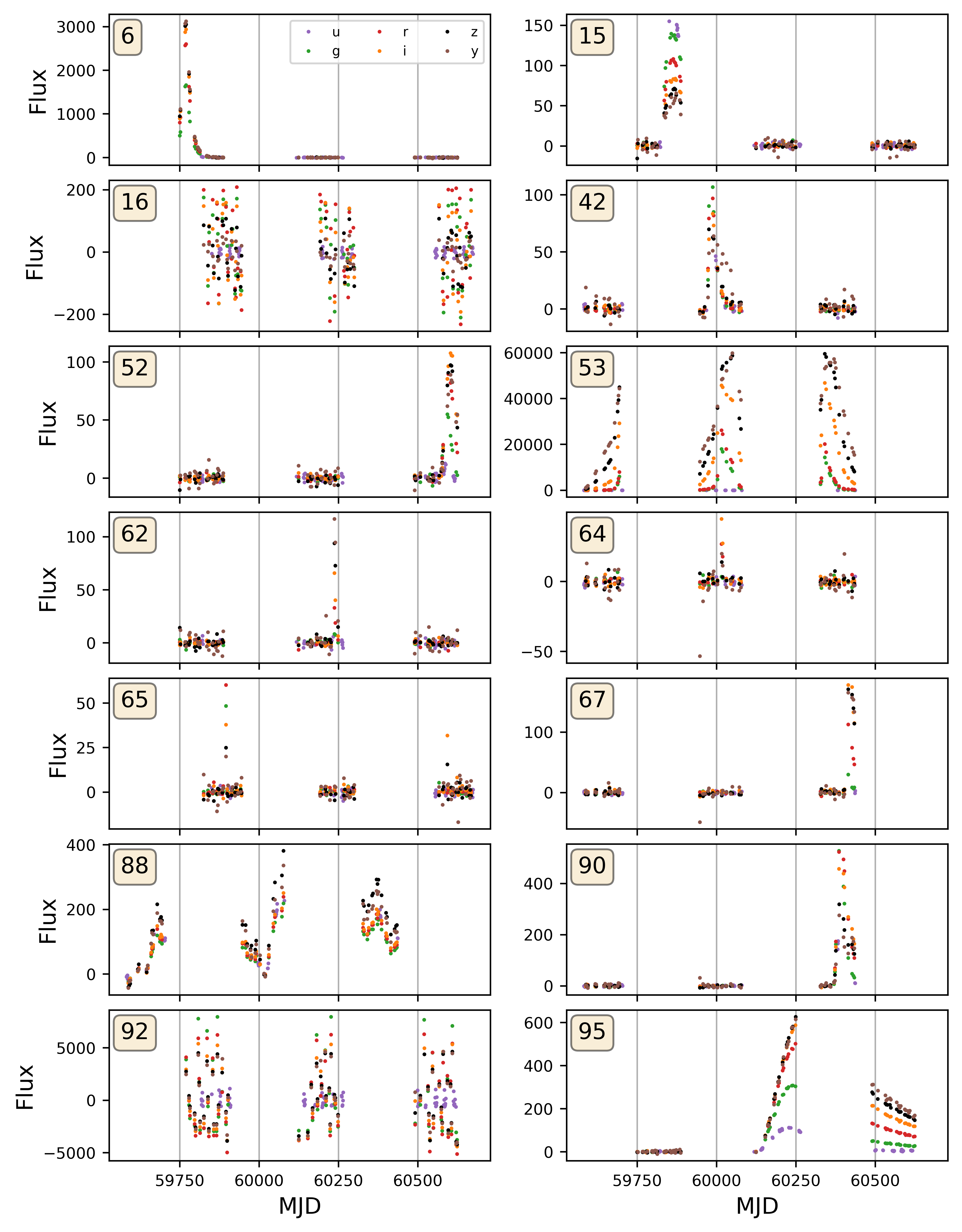
Figure 1: Examples of simulated light curves for each class for DDF mode in the passbands $ugrizy$. MDJ – Modified Julian Date in days

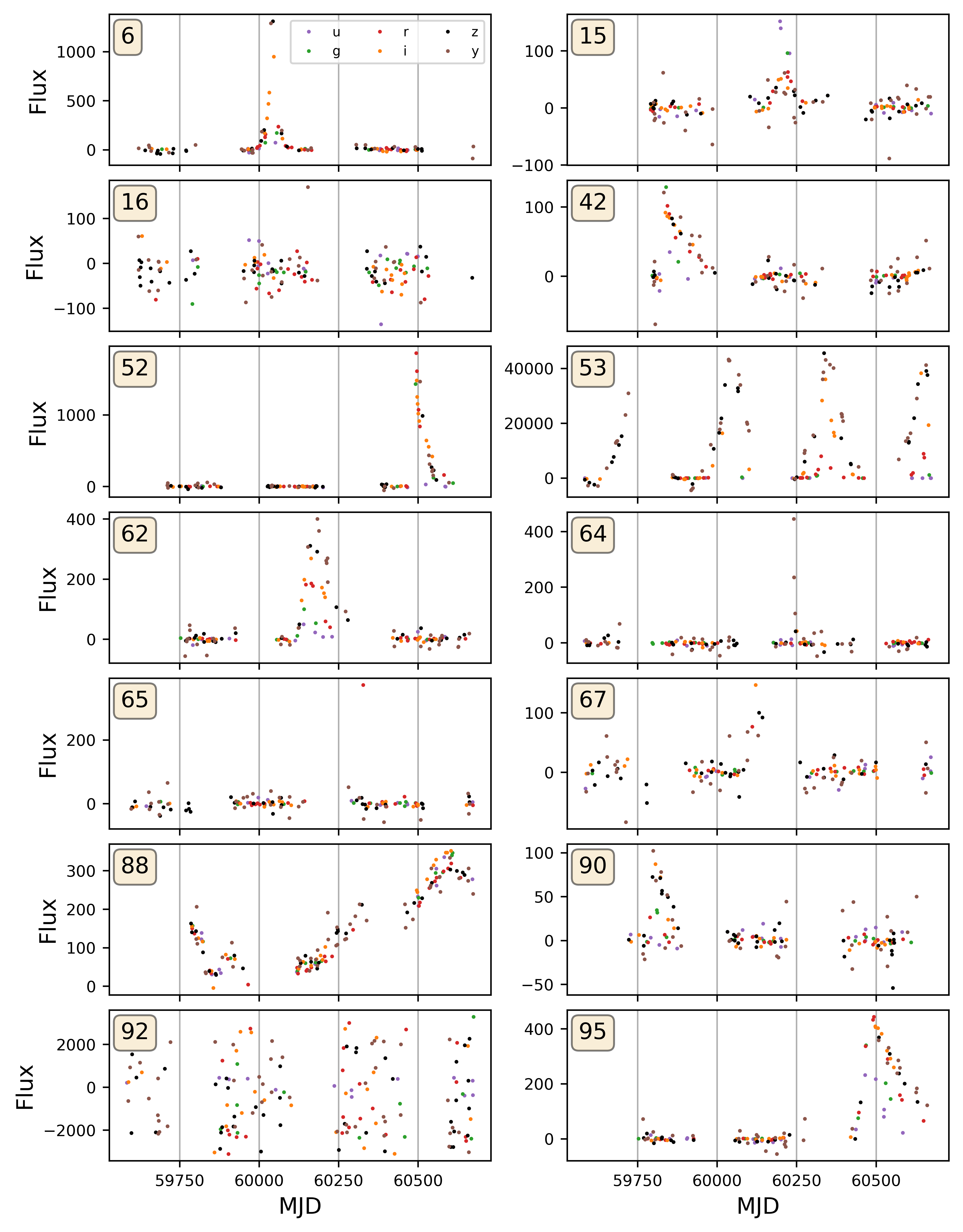
Figure 2: Examples of simulated light curves for each class for WFD mode in the passbands $ugrizy$.

Besides flux values for all 6 passbands, the dataset included flux_err values that simulate measurement errors of the flux (at the $68\%$ confidence interval of the measurement). For extragalactic classes data included the photometric redshifts of the host-galaxies, hostgal-photoz, with their uncertainty, hostgal-photoz-error, the  distance modulus, distmod, and sometimes spectroscopic redshifts, hostgal-specz, if available. Each object was provided with its galactic coordinates, right ascension and the declination, but they did not contribute to the model.

Also, each point had a boolean detected flag. LSST uses a reference image for each position on the sky, a template, and measures the astrophysical sources against the template. Objects for which the total flux from source and background is higher than that of the template have positive flux, and when the total flux is lower than the template flux, they have a negative flux. Due to this difference imaging techniques, objects have to have changed significantly with respect to the template to be detected by LSST. Whether or not they were detected with respect to the template is reported as detected=1. For more details on the metadata provided, see [3].

3 Evaluation

The models were evaluated with weighted multi-class logarithmic loss. Such an arrangement allowed for each class to have roughly equal contribution to the evaluation score. Each object has been labeled with one type. For each object one get a set of predicted probabilities for it to belong to a particular class. The formula used for the evaluation is then defined as follows:

$$\text{Log Loss}=-\left(\frac{\sum^{M}_{i=1}w_{i}\cdot\sum_{j=1}^{N_{i}}\frac{y_{ij}}{N_{i}}\cdot\ln p_{ij}}{\sum^{M}_{i=1}w_{i}}\right),$$ (1)

where $N$ is the number of objects in the class set, $M$ is the number of classes,  $y_{ij}$ is $1$ if observation $i$ belongs to class $j$ and $0$ otherwise, $p_{ij}$ is the predicted probability that observation $i$ belongs to class $j$.

In order to avoid the extremes of the log function, predicted probabilities values are clipped to:

$$\max(\min(p,1-10^{-15}),10^{-15}).$$ (2)

4 Features extraction from photometric light curves

This section details the features extracted to represent light curves. As telescope observations are not always taken at uniformly spaced intervals, the light curve features should be invariant to this non-uniformity.

4.0.1 Statistics

We calculated basic statistics from the light curves and tested all features from the cesium package [13]. The features based on ratios, $median\_absolute\_deviation$, standard deviation ($std$), and skewness ($skew$) were the most useful for classification. The time between the first and the last detected observation ($detected\_time\_diff$), suggested by Dr Grzegorz Sionkowski, is a handy feature helping to separate transient supernova events. The normalized maximum flux values, $norm\_flux\_max\_i$, defined as $max(flux\_i)/max(flux)$, where $i$ denotes the passaband number, also shown high importance for the classifier.

4.0.2 Light curves features from the FEETS package

There is a number of packages for feature extraction from time-series. We tested features from the FEETS package, specially designed for the photometric light curves [14]. $CAR\_sigma$, $CAR\_tau$, and $CAR\_mean$ [15] were particularly helpful, however, required long calculation time. We used the numba package [16] available for python along with minor vectorisation to speed up their calculation $10$x times faster than the original package.

4.0.3 Peaks analysis

For the most well-defined passbands 2, 3, 4, and 5 we look for a single peak if it exists. A peak is searched by a threshold relative to the flux maximum of a passband. We consider the certain peak intervals (with the known flux values) and estimated peak intervals (by linear approximation of flux values). Then we get the aggregated “certain” peak interval by the union of passband “certain” intervals, and wider aggregated “estimated” interval by the intersection of passband “estimated” intervals. The lengths of these two aggregated intervals, $peaks\_certain\_width$ and $peaks\_estimated\_width$, are used as features.

Another common way for peaks analysis is an autocorrelation and cross-correlation. They require equal temporal sampling; therefore, data for the light curves were first re-sampled using linear interpolation, and then the parameters of the autocorrelations were extracted. We used autocorrelation lag $0$ ($autocorrelation$) and autocorrelation peak widths. We tried to extract statistics from the interpolated and re-sampled light curves as well, but it did not bring the model improvement.

4.0.4 Magnitudes

The magnitudes, $M$, were calculated from the measured flux ($F$) and distance modulus, $\mu$, as follows:

$$m=-2.5*log_{10}(\frac{F}{F_{ref}})-\mu,$$ (3)

where $F_{ref}$ is a reference flux. Brighter objects have smaller magnitudes. For the purpose of the challenge, the reference flux was set to $F_{ref}=1$ for all the objects as the reference was not provided.

We tested two sets of magnitude features: calculated for all data points and data points with $detected=1$ only. The latter option gave better results, possibly due to better handling of outliers in the observations. We calculated statistics of magnitudes per passband ($magnitude\_min\_i$, $i=0..5$) and aggregated for all passbands together. The magnitude minimum, $magnitude\_min$, mean, $magnitude\_mean$, standard deviation, $magnitude\_std$, and also integration over the peak, $magnitude\_sum$ shown the highest importance for the classifier (see Table 3). The statistics calculated for individual passbands had a smaller contribution to the classification model accuracy than the aggregated values. The magnitudes were also corrected for the redshift using the following k-correction calculator [17]. It is only valid for relatively small redshifts [18], but the majority of data lie in this region. The k-correction of magnitudes per band did not improve the classification results.

4.0.5 Parametric curve fitting

The main challenge was to separate supernova of different types, classes: 42, 52, 62, 67, and 90. The other classes were well distinguished with the basic features listed above, therefore we focused on the special features to differentiate between supernova types. The parametric curve fitting is a commonly used technique for supernova classification [19, 20, 7, 21].

We tried models from the papers of Bazin et.al. [19], Newling et.al [20], and Karpenka et.al. [7] for features extraction. Besides that, we also calculated the Gaussian fits to define peak-width, and linear decay slope of supernova light curves in the log scale for different passbands, $supernova\_decay\_i$. The root-mean-square loss was one of the most important features in all the curves fittings.

The parametric curve fitting was made in two stages. First, we fit a Gaussian model to a light curve to define an approximate position of the light curve peak:

$$f^{(i)}(t)=f_{m}^{(i)}\cdot e^{-\dfrac{(t-t_{0})^{2}}{2s^{2}}}+f_{0},$$ (4)

where $i=0..5$ is the passband number. The Gaussian width $gauss\_s\_i$ and a root-mean-square fit error, $gauss\_error\_i$, were used as the classifier features.

We defined a penalty function to regularise $t_{0}$, so that band peaks do not wander too far off each other for different passbands:

$$p(\mathbf{t_{0}})=\dfrac{1}{6}\sum_{i}{(t^{(i)}_{0}-\dfrac{1}{6}\sum_{i}{t^{(i)}_{0}})^{2}}.$$ (5)

Secondly, we used a double-phase exponential model [19] with parameters: $f_{0}$, $t_{0}$, $f_{m}$, $\tau_{fall}$, and $\tau_{rise}$:

$$f^{(i)}(t)=f_{m}^{(i)}\cdot\dfrac{e^{-(t-t_{0}^{(i)})/\tau_{fall}}}{1+e^{-(t-t_{0}^{(i)})/\tau_{rise}}}+f_{0},$$ (6)

where $i=0..5$ is the passband number.

The examples of light curves fitted with Eqn.6 are shown in Fig.3 for DDF and WFD samples.

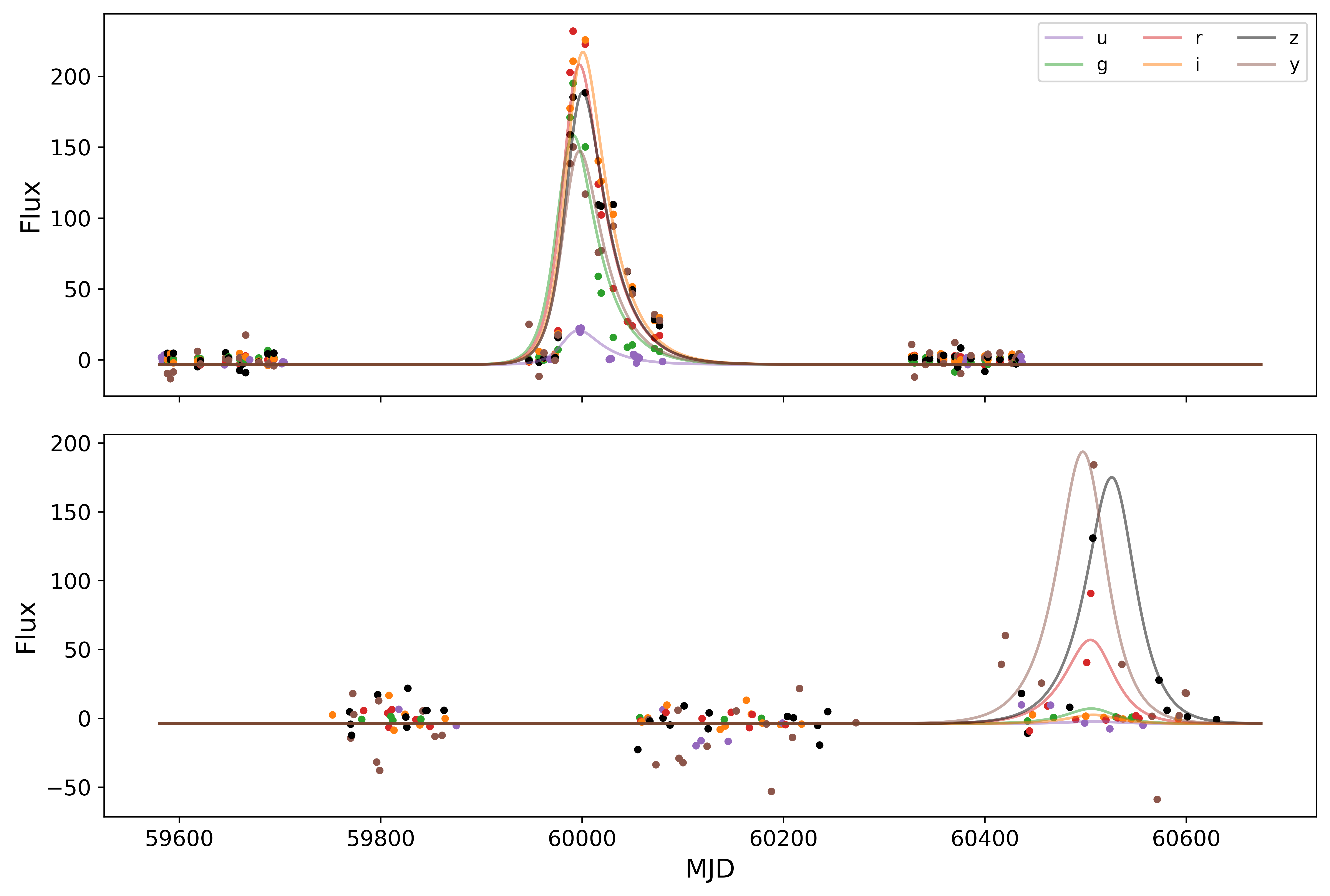
Figure 3: The light curves data (dots) and fitted curves (Eqn.6, lines) for DDF (top) and WFD (bottom) samples.

The fitted parameters, $f_{m}^{(i)}$, $\tau_{fall}$, and $\tau_{rise}$ were used as features for the classifier. The root-mean-square loss of the fits, $Bazin\_fitting\_loss$, was also added as a feature. From the Eqn.6 we derived the position of the peak maximum and found absolute magnitudes from the parametric curve fittings, $magnitude\_fitted\_i$. These fitted magnitude values are particularly useful for the incomplete light curves, where the flux maximum (the minimum of the absolute magnitude) was missed in the observations. We also calculated a range of features from the parametric fits for all 6 passbands: $log(f_{m}^{(i)})$, $m_{15}$ and $m_{-10}$ parameters [22], peak widths at three different levels of $0.2$, $0.5$ and $0.8$ of the flux peak maximum.

4.0.6 Periodograms

We used the Lomb-Scargle algorithm to extract periods from the non-periodic data [23], which is a commonly-used statistical tool designed to detect periodic signals in unevenly-spaced observations. The periods have shown high permutation importance in the features selection process (Table 3). Adding $periods$ yield minor improvement of the model accuracy, which is probably not worth computational times (around two weeks for the test set on 24 CPUs). The dataset mostly consisted of the transients, and the other classes were well defined without Lomb-Scargle periods.

4.0.7 Colours

The astronomical colours were calculated from magnitudes as suggested in [18], both from the measured detected magnitudes ($u\_r$, $u\_z$, etc.) and from the magnitude values found from the parametric curve fits (denoted as $fitted\_u\_z$).

5 Machine learning method

Boosted decision trees are, in general, excellent classifiers, commonly used for time series. Decision trees map input features to output classes using a series of decision rules [11]. The probabilities from each of the decision trees in the ensemble are averaged to produce a final probability. Averaging over a large number of classificators makes this method robust and increases the accuracy of predictions. Boosted decision trees have been successfully applied recently in photometric supernova classification [6].

In this paper, we use python boosted decision trees implementation, LightGBM [12], with $5$ folds cross-validation, stratified by classes. We used different sets of features for the input of LightGBM classifier and selected the optimal features set based on the average 5-folds cross-validation scheme. The output was then tested on a large test dataset ($3479803$ light curves samples) provided in the challenge.

The hyper-parameters optimised for the LightGBM using cross-validation are listed in Table 2.

Parameter	Value	Description
max_depth	3	Maximum tree depth
min_child_samples	50	Minimum number of samples in a child (leaf).
num_leaves	5	Maximum number of tree leaves
learning_rate	0.02	Learning rate
max_bin	40	Max number of bins that feature values will be bucketed in

Table 2: The hyper-parameters used for the LightGBM classifier.

6 Augmentations

The training dataset is relatively small, and augmentations of the light curves were beneficial to reduce overfitting of the classifier. The following augmentations were used:

• We first augmented train $10$x times using flux variation within a normal distribution of the corresponding flux-err values provided. We also applied a similar approach to augment metadata for hostgal-photoz values.

• We introduced a small time shift to bring translation symmetry.

• The train and test data had a different distribution with DDF data ratio of 30% and 1% in the train and test sets, respectively. To overcome over-fitting to the DDF samples, we down-sampled DDF in the current augmentation and re-selected features checking eli5 importance for WFD samples only.

• Finally, we augmented train more, making 30x train from WFD samples and leaving DDF samples only in the original train fold. It gave further improvement to the model performance.

7 Features selection

The features selection is important to reduce overfitting, remove redundant features, and avoid confusing the classifier. The following approaches were used to select the most relevant features for the task:

• We used an automatic tool, recursive feature elimination from sklearn library [24], for the initial optimisation. This tool provides the first approximation of the good features set; however, it requires further manual fine-tuning.

• We used permutation importance from eli5 package to rank features [25], and then removed ones with negative or small importance. The permutation importance is computed as a decrease in the score when feature values are permuted (become noise). A list of the best-ranked features and their permutation importance gain coefficients is shown in Table 3.

• We calculated the Pearson correlation between features and removed redundant one-by-one. Although decision tree models should be immune to correlated features, in practice removing highly correlated features improved the model performance.     Such a manual approach with permutation importance worked out much better than the automatic feature selection.

Rank	Feature	Weight	Rank	Feature	Weight
1	detected_time_diff	0.2140$\pm$0.0187	51	qso_log_chi2_qsonu_0	0.0031$\pm$0.0013
2	hostgal_photoz	0.1119$\pm$0.0250	52	m_15_1	0.0030$\pm$0.0015
3	magnitude_min	0.0485$\pm$0.0147	53	magnitude_sum_3	0.0030$\pm$0.0012
4	Bazin_fitting_loss	0.0280$\pm$0.0078	54	median_absolute_deviation_3	0.0030$\pm$0.0048
5	magnitude_mean	0.0249$\pm$0.0102	55	magnitude_min_2	0.0029$\pm$0.0017
6	flux_ratio_square_skew	0.0219$\pm$0.0063	56	supernova_decay_2	0.0028$\pm$0.0029
7	fm_0	0.0180$\pm$0.0022	57	magnitude_sum_4	0.0028$\pm$0.0014
8	median_absolute_deviation_5	0.0167$\pm$0.0086	58	r_i	0.0028$\pm$0.0007
9	detected_mean	0.0161$\pm$0.0049	59	qso_log_chi2_qsonu_2	0.0027$\pm$0.0010
10	magnitude_std	0.0159$\pm$0.0036	60	magnitude_fitted_5	0.0027$\pm$0.0018
11	gauss_s_2	0.0138$\pm$0.0031	61	flux_skew_1	0.0025$\pm$0.0024
12	gauss_error_5	0.0133$\pm$0.0085	62	autocorrelation	0.0025$\pm$0.0030
13	period	0.0105$\pm$0.0039	63	gauss_s_5	0.0024$\pm$0.0009
14	norm_flux_max_1	0.0102$\pm$0.0060	64	magnitude_mean_0	0.0024$\pm$0.0012
15	norm_flux_max_5	0.0093$\pm$0.0043	65	m_15_2	0.0023$\pm$0.0023
16	median_absolute_deviation_4	0.0089$\pm$0.0084	66	magnitude_mean_4	0.0023$\pm$0.0033
17	tau_fall	0.0088$\pm$0.0038	67	qso_log_chi2_qsonu_5	0.0022$\pm$0.0013
18	fitted_g_i	0.0087$\pm$0.0016	68	magnitude_min_fitted_4	0.0021$\pm$0.0011
19	g_r	0.0085$\pm$0.0016	69	magnitude_min_5	0.0021$\pm$0.0013
20	gauss_s_3	0.0074$\pm$0.0038	70	log_fm_1	0.0020$\pm$0.0028
21	peaks_certain_width	0.0072$\pm$0.0045	71	tau_rise	0.0020$\pm$0.0015
22	CAR_tau	0.0067$\pm$0.0050	72	fitted_u_r	0.0020$\pm$0.0007
23	log_fm_4	0.0064$\pm$0.0019	73	m_15_4	0.0020$\pm$0.0017
24	flux_err_min	0.0064$\pm$0.0092	74	magnitude_sum_0	0.0020$\pm$0.0010
25	magnitude_mean_2	0.0063$\pm$0.0016	75	fm_1	0.0019$\pm$0.0023
26	fitted_g_z	0.0059$\pm$0.0009	76	gauss_s_0	0.0019$\pm$0.0006
27	flux_diff	0.0056$\pm$0.0014	77	magnitude_min_fitted_1	0.0019$\pm$0.0011
28	gauss_s_4	0.0056$\pm$0.0025	78	magnitude_min_4	0.0019$\pm$0.0012
29	peaks_estimated_width	0.0054$\pm$0.0023	79	magnitude_min_fitted_2	0.0018$\pm$0.0014
30	magnitude_sum_2	0.0054$\pm$0.0019	80	freq_varrat_4	0.0018$\pm$0.0026
31	norm_flux_max_0	0.0053$\pm$0.0018	81	magnitude_min_0	0.0018$\pm$0.0008
32	median_absolute_deviation_2	0.0052$\pm$0.0025	82	g_i	0.0018$\pm$0.0009
33	gauss_error_2	0.0051$\pm$0.0026	83	stetson_k_1	0.0016$\pm$0.0010
34	m_15_5	0.0048$\pm$0.0026	84	norm_flux_max_4	0.0016$\pm$0.0005
35	log_fm_5	0.0046$\pm$0.0027	85	r_z	0.0015$\pm$0.0016
36	norm_flux_max_3	0.0045$\pm$0.0030	86	fm_3	0.0015$\pm$0.0009
37	fitted_i_z	0.0042$\pm$0.0018	87	fitted_r_i	0.0014$\pm$0.0009
38	flux_skew_2	0.0042$\pm$0.0023	88	magnitude_mean_3	0.0014$\pm$0.0008
39	gauss_error_1	0.0041$\pm$0.0043	89	g_z	0.0014$\pm$0.0011
40	fitted_r_z	0.0041$\pm$0.0018	90	freq_varrat_1	0.0014$\pm$0.0018
41	magnitude_mean_5	0.0039$\pm$0.0021	91	magnitude_min_1	0.0013$\pm$0.0007
42	fm_5	0.0036$\pm$0.0018	92	flux_skew	0.0013$\pm$0.0014
43	gauss_err_4	0.0036$\pm$0.0047	93	gauss_error_3	0.0013$\pm$0.0015
44	fm_2	0.0034$\pm$0.0016	94	qso_log_chi2_qsonu_1	0.0012$\pm$0.0005
45	i_z	0.0033$\pm$0.0014	95	magnitude_mean_1	0.0012$\pm$0.0009
46	norm_flux_max_2	0.0032$\pm$0.0028	96	CAR_sigma	0.0011$\pm$0.0017
47	m_15_3	0.0032$\pm$0.0017	97	log_fm_0	0.0010$\pm$0.0019
48	gauss_s_1	0.0032$\pm$0.0019	98	fitted_g_r	0.0010$\pm$0.0007
49	supernova_decay_3	0.0031$\pm$0.0013	99	u_r	0.0009$\pm$0.0014
50	magnitude_sum_5	0.0031$\pm$0.0019	100	flux_skew_3	0.0009$\pm$0.0017

Table 3: A list of the best ranked features and their permutation importance coefficients.

8 Results

The weighted logarithmic loss values for different sets of features used with LightGBM classifier are presented in Table 4 for 5-fold cross-validation and test data (the smaller the better).

Features set	Augmentations	Log Loss, 5 folds	Log Loss, test
All features (167)	10x augs	0.52209	0.59910
Top 50 features	10x augs	0.52756	0.60863
Top 100 features	10x augs	0.51769	0.59770
Selected features (82)	10x augs	0.51588	0.59524
Top 100 features	no augs	0.44487	0.62834
Selected features (82)	no augs	0.44036	0.63164
Selected features (82)	30x augs	0.51720	0.58788

Table 4: The model metric results for different sets of features.

The evaluation metric, logarithmic loss, depended on the number of features included for the LightGBM classifier, with all (167) and too few features (top 50) giving the worst results. Including top $100$ features from the permutation importance ranking gave nearly optimal results. Removing the redundant features using Pearson correlation helped to improve the model accuracy further. The selected features set for the best model is listed in Table 5. Train set augmentation improved significantly model loss values between $0.63164$ and $0.58788$ for the test set. The cross-validation loss values were larger with augmentations, but it reduced overfitting giving better results on the test set.

Selected features
$detected\_time\_diff$, $hostgal\_photoz$, $magnitude\_min$, $magnitude\_mean$,
$magniude\_std$, $magnitude\_min\_i,i=0..5$, $magnitude\_mean\_i,i=2..5$,
$CAR\_tau$, $flux\_err\_min$, $norm\_flux\_max\_i,i=0..5$,
$Bazin\_fitting\_loss$, $tau\_fall$, $tau\_rise$, $fm\_i,i=0..5$, $log\_fm\_i,i=1,4,5$,
$flux\_ratio\_square\_skew$, $flux\_skew$, $flux\_skew\_1$, $flux\_skew\_2$, $flux\_diff$,
$median\_absolute\_deviation\_5$, $median\_absolute\_deviation\_2$, $detected\_mean$,
$peaks\_certain\_width$, $peaks\_estimated\_width$, $percent\_close\_to\_median\_2$,
$gauss\_s\_i,i=0..5$, $gauss\_error\_i,i=0..5$, $supernova\_decay\_3$,
$qso\_log\_chi2\_qsonu\_0$, $freq\_varrat\_1$, $freq\_varrat\_4$, $stetson\_k\_3$,
$magnitude\_fitted\_i,i=1,2,4$, $autocorrelation$, $periods$
$g\_r$, $g\_i$, $r\_z$, $r\_i$, $g\_z$, $u\_r$, $i\_z$,
$fitted\_g\_r$, $fitted\_g\_i$, $fitted\_r\_z$, $fitted\_r\_i$, $fitted\_g\_z$, $fitted\_u\_r$, $fitted\_i\_z$

Table 5: The list of selected features set for the best model

The confusion matrix of the predictions for the best model with 5-folds cross-validation is shown in Fig. 4 The most problematic classes were supernova classes, showing the confusion of the classifier between different supernova types, especially for class 52 (SN Iax type). The other classes were well distinguished with the high accuracy of 88-100% using the selected set of features. The model was tested on a large test dataset, giving one of the top results in the challenge.

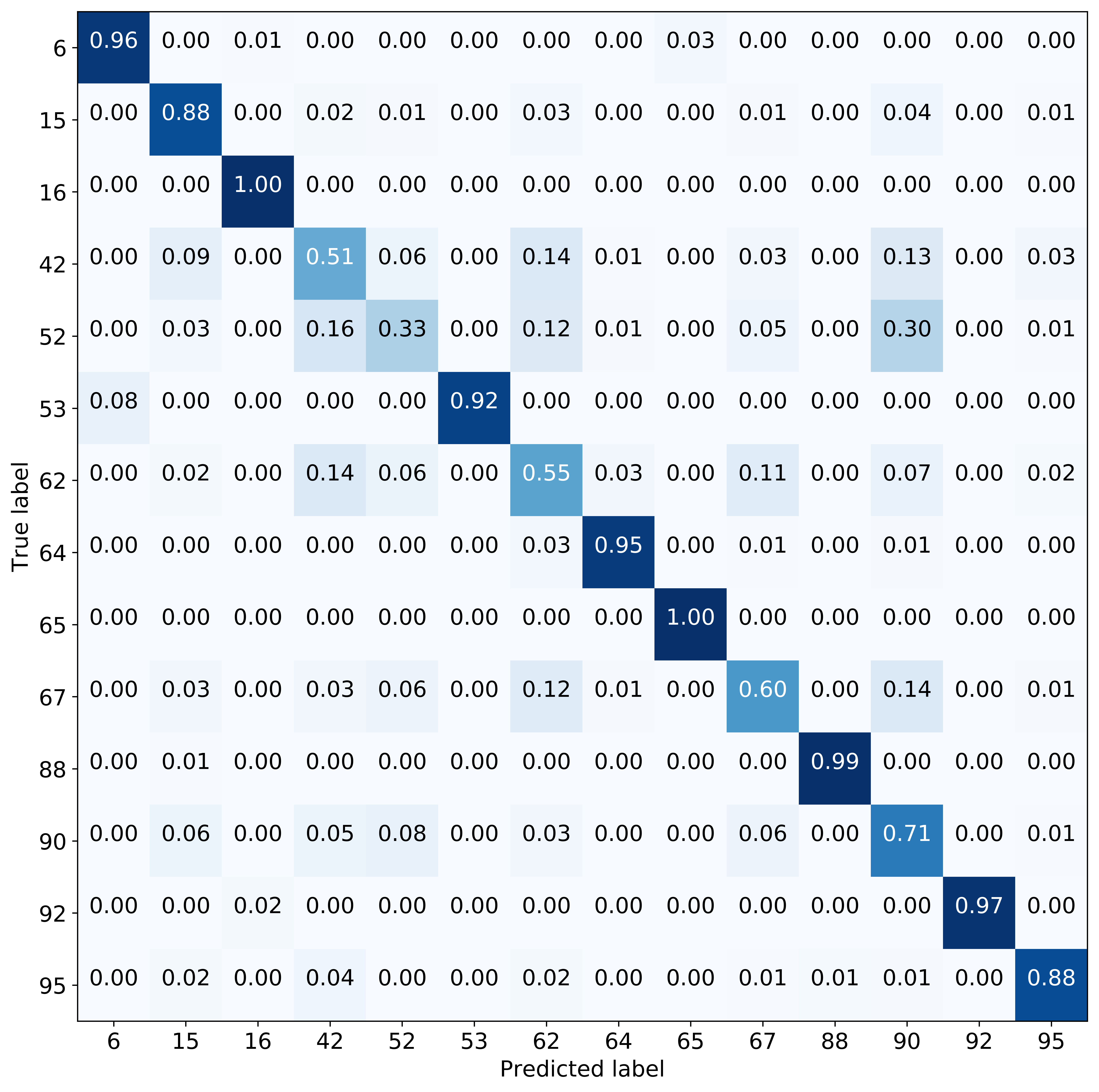
Figure 4: The confusion matrix of the predictions for the best model with 5-folds cross-validation.

9 Discussion

There was a range of other experiments that we tried, but it did not help to increase the accuracy of the model. Nevertheless, we list those unsuccessful attempts here, as we believe it might be useful information for others.

9.0.1 Autoencoders

We tried to use variational autoencoders to extract features from the light curves and use them for the classifier. We encoded the light curves in $43-50$ features; however, none of then gave improvement to the classifier when adding to the selected features set.

9.0.2 Multiple parametric curve fittings

We used several parametric fits from the papers of Bazin et.al. [19], Newling et.al. [20], and Karpenka et.al. [7] to fit supernova rise and decay times. Using the aggregated rise and decay times gave the same accuracy than using individual values per passband. Adding parameters from several different fits together (i.e., form  Bazin et.al. [19] and Karpenka et.al. [7]) did not bring improvement on classification, so that only single fit was sufficient. Based on the features selection process, we used Bazin et.al. fit [19] for the final features set.

10 Conclusion

Here we present the model for the automatic photometric classification of the various astronomical objects. The model was developed in the context of the PLAsTiCC astrological challenge and achieved one of the top results in the competition.

Often, the solutions of machine learning competitions are based on extensive and diverse ensembles, test-time augmentation, and pseudo labeling, which is not always possible and feasible in real-life applications. We propose a solution based on the simple LightGBM model, feature extraction and augmentation.

We calculated and tested numerous features from the light curves and metadata. All features were ranked with permutation importance algorithm, and the most relevant were used for the classification (see Table 3). We used the boosted decision trees LightGBM model and 5-folds cross-validation. Too many features lead to overfitting of the classifier, while too few are insufficient to achieve a good model accuracy. Selecting around $100$ features seemed to be close to the golden middle for this task. Removing redundant features manually with Pearson correlation also improved the result. The features selection process is outlined in section 7. Augmentations described in section 4 also helped to reduce overfitting and improve model accuracy. The final results and selected features are shown in Table 4 and Table 5, respectively.

We archived high accuracy of 88-100% for classification for all astronomical object, except for the supernova classes: 42, 52, 62, 67, and 90. Supernova types classification accuracy varied between 33-71%, with class 52 (SN Iax) being the most undefined. The confusion between different supernova types persisted, which indicates that other approaches would be desirable for these types. For instance, it could be beneficial to separate supernova types from the other objects and use an additional classifier for them and also introduce template fittings, similar to Type I [26], for all supernova types.

11 Acknowledgements

The authors thank the challenge organisers, Dr Olivier Grellier for the introductory baseline [27], Dr Grzegorz Sionkowski for suggesting one of the top features for the classifier, Kyle Boone, Dr Jean-François Puget (known as CPMP) and Open Data Science community (ods.ai) for useful discussions.

References

- [1] https://www.lsst.org/.
- [2] R. Kessler, G. Narayan, A. Avelino, E. Bachelet, R. Biswas, P. J. Brown, D. F. Chernoff, A. J. Connolly, M. Dai, S. Daniel, R. Di Stefano, M. R. Drout, L. Galbany, S. González-Gaitán, M. L. Graham, R. Hložek, E. E. O. Ishida, J. Guillochon, S. W. Jha, D. O. Jones, K. S. Mandel, D. Muthukrishna, A. O’Grady, C. M. Peters, J. R. Pierel, K. A. Ponder, A. Prša, S. Rodney, and V. A. Villar and. Models and simulations for the photometric LSST astronomical time series classification challenge (PLAsTiCC). Publications of the Astronomical Society of the Pacific, 131(1003):094501, jul 2019.
- [3] https://www.kaggle.com/michaelapers/the-plasticc-astronomy-starter-kit.
- [4] Alex Malz, Renée Hložek, Tarek Allam Jr, Anita Bahmanyar, Rahul Biswas, Mi Dai, Lluís Galbany, Emille Ishida, Saurabh Jha, David Jones, Rick Kessler, Michelle Lochner, Ashish Mahabal, Kaisey Mandel, Rafael Martínez-Galarza, Jason McEwen, Daniel Muthukrishna, Gautham Narayan, Hiranya Peiris, Christina Peters, Christian Setzer, The LSST Dark Energy Science Collaboration, The LSST Transients, and Variable Stars Science Collaboration. The photometric lsst astronomical time-series classification challenge (plasticc): Selection of a performance metric for classification probabilities balancing diverse science goals. 2018.
- [5] Joseph W. Richards, Dan L. Starr, Nathaniel R. Butler, Joshua S. Bloom, John M. Brewer, Arien Crellin-Quick, Justin Higgins, Rachel Kennedy, and Maxime Rischard. On machine-learned classificatiob of variable stars with sparse and noisy time-series data. The Astrophysical Journal, 733(1):10, apr 2011.
- [6] Michelle Lochner, Jason D. McEwen, Hiranya V. Peiris, Ofer Lahav, and Max K. Winter. Photometric supernova classification with machine learning. The Astrophysical Journal Supplement Series, 225(2):31, aug 2016.
- [7] N. V. Karpenka, F. Feroz, and M. P. Hobson. A simple and robust method for automated photometric classification of supernovae using neural networks. Monthly Notices of the Royal Astronomical Society, 429(2):1278–1285, dec 2012.
- [8] https://www.kaggle.com/c/PLAsTiCC-2018/overview.
- [9] The PLAsTiCC team, Tarek Allam Jr., Anita Bahmanyar, Rahul Biswas, Mi Dai, Lluís Galbany, Renée Hložek, Emille E. O. Ishida, Saurabh W. Jha, David O. Jones, Richard Kessler, Michelle Lochner, Ashish A. Mahabal, Alex I. Malz, Kaisey S. Mandel, Juan Rafael Martínez-Galarza, Jason D. McEwen, Daniel Muthukrishna, Gautham Narayan, Hiranya Peiris, Christina M. Peters, Kara Ponder, Christian N. Setzer, The LSST Dark Energy Science Collaboration, The LSST Transients, and Variable Stars Science Collaboration. The photometric lsst astronomical time-series classification challenge (plasticc): Data set, 2018.
- [10] https://www.kaggle.com/mithrillion/all-classes-light-curve-characteristics-updated.
- [11] J. Ross Quinlan. Learning efficient classification procedures and their application to chess end games. In Machine Learning, pages 463–482. Springer Berlin Heidelberg, 1983.
- [12] https://lightgbm.readthedocs.io/en/latest/Python-Intro.html.
- [13] https://github.com/cesium-ml/cesium.
- [14] https://feets.readthedocs.io/en/latest/tutorial.html.
- [15] K. Pichara, P. Protopapas, D.-W. Kim, J.-B. Marquette, and P. Tisserand. An improved quasar detection method in EROS-2 and MACHO LMC data sets. Monthly Notices of the Royal Astronomical Society, 427(2):1284–1297, nov 2012.
- [16] https://numba.pydata.org/.
- [17] http://kcor.sai.msu.ru/getthecode/.
- [18] Richard Beare, Michael J. I. Brown, and Kevin Pimbblet. An accurate new method of calculating absolute magnitudes and k-corrections applied to the sloan filter set. The Astrophysical Journal, 797(2):104, dec 2014.
- [19] G. Bazin, N. Palanque-Delabrouille, J. Rich, V. Ruhlmann-Kleider, E. Aubourg, L. Le Guillou, P. Astier, C. Balland, S. Basa, R. G. Carlberg, A. Conley, D. Fouchez, J. Guy, D. Hardin, I. M. Hook, D. A. Howell, R. Pain, K. Perrett, C. J. Pritchet, N. Regnault, M. Sullivan, P. Antilogus, V. Arsenijevic, S. Baumont, S. Fabbro, J. Le Du, C. Lidman, M. Mouchet, A. Mourão, and E. S. Walker. The core-collapse rate from the supernova legacy survey. Astronomy & Astrophysics, 499(3):653–660, apr 2009.
- [20] J. Newling, M. Varughese, B. Bassett, H. Campbell, R. Hlozek, M. Kunz, H. Lampeitl, B. Martin, R. Nichol, D. Parkinson, and M. Smith. Statistical classification techniques for photometric supernova typing. Monthly Notices of the Royal Astronomical Society, 414(3):1987–2004, apr 2011.
- [21] S. Gonzalez-Gaitan, N. Tominaga, J. Molina, L. Galbany, F. Bufano, J. P. Anderson, C. Gutierrez, F. Forster, G. Pignata, M. Bersten, D. A. Howell, M. Sullivan, R. Carlberg, T. de Jaeger, M. Hamuy, P. V. Baklanov, and S. I. Blinnikov. The rise-time of type II supernovae. Monthly Notices of the Royal Astronomical Society, 451(2):2212–2229, jun 2015.
- [22] F. Taddia, J. Sollerman, G. Leloudas, M. D. Stritzinger, S. Valenti, L. Galbany, R. Kessler, D. P. Schneider, and J. C. Wheeler. Early-time light curves of type ib/c supernovae from the SDSS-II supernova survey. Astronomy & Astrophysics, 574:A60, jan 2015.
- [23] J. D. Scargle. Studies in astronomical time series analysis. II - statistical aspects of spectral analysis of unevenly spaced data. The Astrophysical Journal, 263:835, dec 1982.
- [24] https://scikit-learn.org/stable/modules/generated/sklearn.feature_selection.RFE.html.
- [25] https://eli5.readthedocs.io/en/latest/blackbox/permutation-importance.html.
- [26] J. Guy, P. Astier, S. Baumont, D. Hardin, R. Pain, N. Regnault, S. Basa, R. G. Carlberg, A. Conley, S. Fabbro, D. Fouchez, I. M. Hook, D. A. Howell, K. Perrett, C. J. Pritchet, J. Rich, M. Sullivan, P. Antilogus, E. Aubourg, G. Bazin, J. Bronder, M. Filiol, N. Palanque-Delabrouille, P. Ripoche, and V. Ruhlmann-Kleider. SALT2: using distant supernovae to improve the use of type ia supernovae as distance indicators. Astronomy & Astrophysics, 466(1):11–21, feb 2007.
- [27] https://www.kaggle.com/ogrellier/plasticc-in-a-kernel-meta-and-data.