Effective Rankine-Hugoniot conditions for shock waves in periodic media

Abstract

Solutions of first-order nonlinear hyperbolic conservation laws typically develop shocks in finite time even from smooth initial conditions. However, in heterogeneous media with rapid spatial variation, shock formation may be delayed or avoided. When shocks do form in such media, their speed of propagation depends on the material structure. We investigate conditions for shock formation and propagation in heterogeneous media. We focus on the propagation of plane waves in two-dimensional media with a periodic structure that changes in only one direction. We propose an estimate for the speed of the shocks that is based on the Rankine-Hugoniot conditions applied to a leading-order homogenized (constant coefficient) system. We verify this estimate via numerical simulations using different nonlinear constitutive relations and layered and smoothly varying media with a periodic structure. In addition, we discuss conditions and regimes under which shocks form in this type of media.

1 Introduction

Many important physical phenomena are modeled by first-order nonlinear hyperbolic conservation laws; important examples include water waves and fluid dynamics. It is well known that solutions of such equations generically develop singularities (shocks) in finite time and eventually dissipate all energy. This was shown rigorously for unbounded homogeneous domains with compact initial data in [21, 22].

There are, however, mechanisms that can impede the formation of shocks. For instance, the effect of random topography on shallow water waves was studied in [10, 11], where it is shown to lead to an effective viscosity. As a result, waves over random topography propagate over longer distances before breaking.

For gas dynamics in a periodic domain, there seem to be solutions that remain regular for long times; see [30, 26]. Indeed, in [30] it was conjectured, based on numerical experiments, that in a periodic domain there exist nontrivial solutions in which no singularity forms. These solutions were referred to as NBAT (non-breaking for all time).

One may also consider a setting in which the medium properties vary periodically in space but the solution itself is not assumed periodic. This is what is meant by the phrase periodic medium in the present work. This situation arises naturally in applications that include photonic [12] and phononic crystals [17, 24] and even coastal engineering [5, 34]. The periodic variation in the medium leads to an effective dispersion [29] for linear waves. Nonlinear waves in a periodic medium were studied in [20], where the authors derived via asymptotic expansions an effecitve constant coefficient system of PDEs, whose leading order terms capture the macroscopic behavior of the solution. The lowest-order terms match those of the original system, but with spatially averaged coefficients, while the higher-order terms are dispersive.

In [30] and [10, 11, 29, 20], regularization seems to be the result of reflection; in the first case due to resonant interactions between characteristic fields and in the rest due to reflections caused by the medium itself, which lead to dissipative and/or dispersive effects. In all these references, the authors focused on waves in one space dimension. In the present work we consider an unbounded two-dimensional domain that varies periodically in one direction; see Figure 1. This scenario has been studied already in [28] for linear waves and in [15] for nonlinear waves. In the last reference, a different sort of regularization was observed that does not seem to be caused by reflection, showing that apparently NBAT solutions can arise even when reflective effects are essentially absent.

These mechanisms that prevent or delay the formation of shocks in [10, 11, 20, 15] depend on the initial data and the properties of the medium (i.e., the strengh of the changes in the coefficients, topography, etc.). It is, therefore, possible for shocks to still appear if the induced regularization is not strong enough. Two natural questions arise:

• What properties of the initial data and the medium determine whether solutions exhibit shocks or are NBAT?

• When shocks form, what is their speed of propagation?

For one-dimensional layered media, this was studied in [16], where it was conjectured (based on numerical experiments) that NBAT solutions also exist. The maximum amplitude of initial data leading to NBAT solutions there was related to the properties of the medium. It was also demonstrated numerically that initially discontinuous data could become regular (or almost regular) in such media if the initial discontinuities did not satisfy a certain effective Lax-entropy condition. For shocks that do satisfy this condition, the authors proposed (and verified numerically) a simple expression for the speed of propagation.

Our goal is to extend the results in [16] to the more general two-dimensional situation depicted in Figure 1. To answer question (ii), we assume that the regularization is not strong enough, which leads to the formation of shocks. We propose and test numerically a simple expression for the propagation of shocks in this type of medium. In regard to question (i), we present a range of experimental results but only a partial answer, valid in a more restricted class of media. In the conclusion we discuss a potential research path to obtain such a condition for more general media.

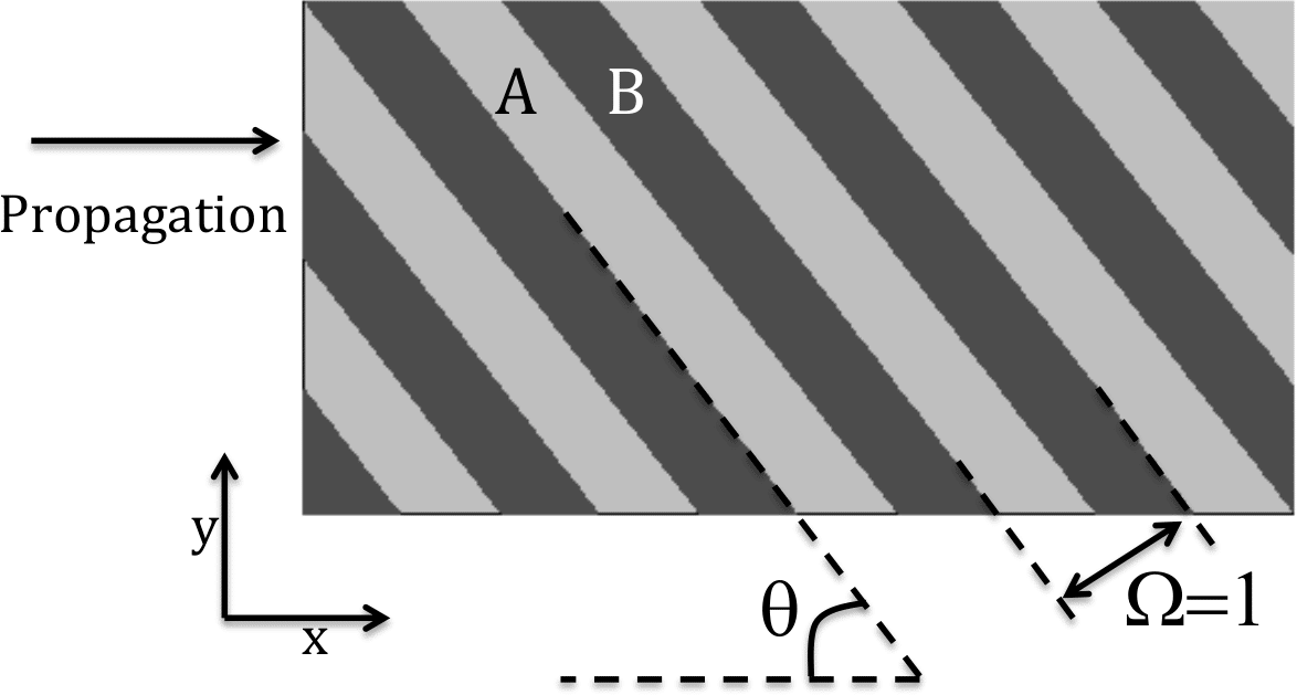
Figure 1: Wave propagation in a layered medium in two dimensions. The domain shown is repeated periodically and extends infinitely in both directions. The orientation of the medium relative to the initial plane wave is given by the angle $\theta$. If $\theta=90^{\circ}$ we refer to the propagation as transverse to the material heterogeneity and if $\theta=0^{\circ}$ we refer to the propagation as parallel.

We remark that linear wave propagation in a layered medium like that of Figure 1 is well studied. Due to the layering, the leading-order effective speed of propagation depends on the angle; see e.g. [25]. Regarding the dispersion of linear waves in layered media, see e.g. [33, 32, 29, 28, 7].

The rest of this manuscript is organized as follows. In §1.1 we present the system of equations and the type of media that we consider. In §1.2 we discuss differences between viscous and dispersive shocks. In §1.3, 1.4 and 1.5 we review the different types of dispersive effects that are induced in periodic media and, for a particular case, discuss the speed of propagation of shocks proposed in [16]. In §2 we use homogenization theory to derive a leading order constant-coefficient system that captures the main macroscopic features of the solution. In §3 we propose an effective shock speed by applying the Rankine-Hugoniot conditions to the homogenized system. This estimate agrees with [16] when $\theta=90^{\circ}$. We test this estimate via numerical experiments, considering two different nonlinearities and two types of periodic media. In §4 we discuss possible conditions for a shock to propagate without being regularized by the induced dispersion. Finally, in §5 we present some conclusions and open questions, with possible approaches to resolve them.

1.1 Governing equations and material configuration

We consider the scalar, nonlinear, variable-coefficient wave equation

$$\epsilon_{tt}-\nabla\cdot\left(\frac{1}{\rho({\bf x})}\nabla\sigma(\epsilon,{\bf x})\right) =0.$$ (1)

We use the notation of elasticity for consistency with related work [20, 16, 28, 15]. Therefore $\epsilon$ denotes strain, $\rho$ density, and $\sigma$ stress. Furthermore, let $K({\bf x})$ denote the bulk-modulus. We consider nonlinear stress-strain relations of the form

$$\sigma(\epsilon,{\bf x})=\hat{\sigma}(K({\bf x})\epsilon),$$ (2)

such that $\sigma_{\epsilon}$ can be expressed as $\sigma_{\epsilon}=G(\sigma)K$ for some function $G(\sigma)$. This condition is needed during the homogenization process in §2. Note that this can be achieved if $\hat{\sigma}\in\mathcal{C}^{1}(K\epsilon)$ (i.e., if $\hat{\sigma}$ is once differentiable with respect to $K\epsilon$) and $\hat{\sigma}$ is one-to-one.

Solutions of (1) with nonlinear stress-strain relations may involve shock singularities. In order to determine entropy-satisfying weak solutions, we write (1) as a first-order hyperbolic system in conservation form:

$${\bf q}_{t}+{\bf f}({\bf q},{\bf x})_{x}+{\bf g}({\bf q},{\bf x})_{y}={\bf 0},$$ (3a)

where

$${\bf q} =\begin{bmatrix}\epsilon\\ \rho({\bf x})u\\ \rho({\bf x})v\end{bmatrix}, {\bf f}({\bf q},{\bf x}) =\begin{bmatrix}-u\\ -\sigma(\epsilon,{\bf x})\\ 0\end{bmatrix}, {\bf g}({\bf q},{\bf x}) =\begin{bmatrix}-v\\ 0\\ -\sigma(\epsilon,{\bf x})\end{bmatrix}.$$ (3b)

Here $u$ and $v$ are the $x$- and $y$-components of velocity, ${\bf q}$ is the vector of conserved quantities, and ${\bf f},{\bf g}$ are the components of the flux in the $x$- and $y$-directions respectively. Note that (for simplicity) we concentrate on two dimensional waves but the results we present can be readily extended to three dimensions. We remark that system (3) is a two-dimensional generalization of the $p$-system from Lagrangian gas dynamics (see e.g. [19, Section 2.13]).

The medium is periodic and extends infinitely in both coordinate directions, as shown in Figure 1. We consider both layered and smoothly-varying media. The smoothly-varying medium is given by

$$K({\bf x}) =\frac{K_{A}+K_{B}}{2}+\frac{K_{A}-K_{B}}{2}\sin(2\pi\xi({\bf x})),$$ (4a)

$$\rho({\bf x}) =\frac{\rho_{A}+\rho_{B}}{2}+\frac{\rho_{A}-\rho_{B}}{2}\sin(2\pi\xi({\bf x})),$$ (4b)

where $K_{A}$, $\rho_{A}$, $K_{B}$ and $\rho_{B}$ are strictly positive constants and $\xi({\bf x})=x\sin\theta+y\cos\theta$. The layered medium, which is composed of two types of materials: $A$ and $B$, is given by

$$(K({\bf x}),\rho({\bf x})) =\begin{cases}(K_{A},\rho_{A})&\text{ if }\sin(2\pi\xi({\bf x}))\geq 0\\ (K_{B},\rho_{B})&\text{ if }\sin(2\pi\xi({\bf x}))<0.\\ \end{cases}$$ (5)

Important properties of the medium are characterized by the linearized impedance $Z({\bf x}):=\sqrt{K\rho}$ and sound speed $c({\bf x}):=\sqrt{K/\rho}$. Variations in $Z$ govern reflection, while $c$ dictates the speed of propagation of small amplitude waves. As we explain in §1.3 and 1.4, different sources of dispersion are induced due to changes in the impedance and sound speed. In some of the numerical experiments that we perform we define $K_{A}$, $\rho_{A}$, $K_{B}$ and $\rho_{B}$ by selecting the values of $Z_{A}:=\sqrt{K_{A}\rho_{A}}$, $c_{A}:=\sqrt{K_{A}/\rho_{A}}$, $Z_{B}:=\sqrt{K_{B}\rho_{B}}$ and $c_{B}:=\sqrt{K_{B}/\rho_{B}}$.

1.1.1 Normalization of the material parameters

Since the stress-strain relation $\sigma=\hat{\sigma}(K\epsilon)$ is a function of the product $K\epsilon$, we can normalize the parameters with respect to $(K_{A},\rho_{A})$. As a result, we can consider without loss of generality $(K_{A},\rho_{A})=1$. To see this, let

$$\tilde{K}({\bf x}) =K({\bf x})/K_{A},$$ (6a)

$$\tilde{\rho}({\bf x}) =\rho({\bf x})/\rho_{A}.$$ (6b)

Multiply (1) by $K_{A}$ and use (6) to obtain

$$(K_{A}\epsilon)_{tt}-\nabla\cdot\left[\frac{1}{\tilde{\rho}({\bf x})}\nabla\left(\frac{K_{A}}{\rho_{A}}\hat{\sigma}\left(\tilde{K}({\bf x})K_{A}\epsilon\right)\right)\right] =0.$$ (7)

Finally, let $\tilde{\epsilon}=K_{A}\epsilon$ and $\tilde{\sigma}=\frac{K_{A}}{\rho_{A}}\hat{\sigma}\left(\tilde{K}({\bf x})K_{A}\epsilon\right)=\frac{K_{A}}{\rho_{A}}\sigma$ to obtain

$$\tilde{\epsilon}_{tt}-\nabla\cdot\left[\frac{1}{\tilde{\rho}({\bf x})}\nabla\tilde{\sigma}\left(\tilde{K}({\bf x})\tilde{\epsilon}\right)\right]=0.$$ (8)

This equation has the same form as (1), but with $\tilde{\rho}_{A}=\tilde{K}_{A}=1$ and the parameters in the $B$-material scaled accordingly. Henceforth, we omit the tildes and assume $(K_{A},\rho_{A})=1$ whenever convenient.

1.2 Viscous versus dispersive shocks

In contrast to first-order hyperbolic conservation laws, higher-order PDE models often include viscous or dispersive terms that prevent the formation of discontinuities and lead instead to what are known as viscous shocks or dispersive shocks. Viscous and dispersive shocks have very different structures and are typically treated with different mathematical tools. Viscous shocks connect two states via a narrow, smooth transition region and generate an increase in physical entropy over time. The speed of a viscous shock is given by the Rankine-Hugoniot condition which is a consequence of the conservation laws themselves [18]. A dispersive shock, on the other hand, connects two states by an oscillatory region that expands in time. Dispersive shocks do not generate entropy. The speed of the leading edge of a dispersive shock is related to the speed of a solitary wave, while the speed of the trailing edge is related to that of small-amplitude perturbations. The regularization observed in [29, 20, 16, 28, 15] and in the present work can be related to dispersive regularization occurring in higher-order dispersive wave models. In particular, as explained in [29], the periodic structure of the medium leads to an effective dispersion of waves. We refer to [13] for a detailed discussion about viscous and dispersive shocks, to [36] for the main mathematical tools to treat dispersive shocks, and to [6] for a review of the theory of dispersive shocks. We remark that randomly varying media seem to lead to viscous, rather than dispersive, effective equations; see for example [31, 10, 11].

Numerical methods for first-order hyperbolic conservation laws are designed to approximate the vanishing-viscosity limit of a viscously-regularized system. Thus they impose the Rankine-Hugoniot conditions and attempt to approximate viscous shocks in the limit where the width of the shock region vanishes (i.e., the viscous shock becomes a discontinuity). In practice, any stable numerical method must impose some viscosity in the shock region and so the shock is approximated by a region of finite width. Hence the solutions presented herein are affected by an interplay of viscous (numerical) and dispersive (from the medium) effects. By refining the computational mesh, numerical viscosity can be reduced and thus it is possible in principle to determine whether the solution to the first-order variable-coefficient system (with no viscosity) is in fact NBAT. We follow the methodology of [16], distinguishing non-dispersive shocks by the presence of an increase in physical entropy that persists when the mesh is refined.

Figure 2 demonstrates the range of possible behaviors. Each plot shows a solution corresponding to propagation of an initial square (plane) wave in a periodic layered medium; the only difference between the plots is $\theta$, the orientation of the plane wave relative to the medium. Depending on the medium properties and angle of propagation, one may observe shock formation (top left), dispersive shock formation followed by the creation of solitary waves (top right) or more complicated behavior that lies between these extremes (bottom row).

Figure 2: Examples of wave propagation in a layered medium (5). Differences in material properties and angle of propagation can lead to behavior that is dominated by shock formation or by dispersion. The material coefficients are $c_{A}=1$, $c_{B}=4$ and $Z_{A}=Z_{B}=1$ and the angle of propagation is: (top-left) $\theta=90^{\circ}$, (top-right) $\theta=0^{\circ}$, (bottom-left) $\theta=45^{\circ}$ and (bottom-right) $\theta=67.5^{\circ}$. The dashed red line shows, for reference, the behavior in a homogeneous medium with appropriately averaged properties (see §2). The initial condition is an effective purely right-going shock given by (28) with $x_{s}=20$, $u_{l}$ given by (27), $u_{r}=0$, $\sigma_{l}=1$ and $\sigma_{r}=0$. We show the solution at $t=25$ and use the nonlinear stress-strain relation (29a).

1.3 $Z$-dispersion: effective dispersion induced by reflections

Consider a plane wave traveling transversely in a layered medium; i.e. let $\theta=90^{\circ}$ in Figure 1. In this case its propagation follows the theory developed in [16], which we briefly review here. If the impedance is mismatched, reflections occur at each interface. The net effect of these reflections is macroscopic dispersion, as shown in [29] via Bloch expansions and in [9, 4, 3, 37] via homogenization theory. When the material parameters change such that the linearized impedance remains constant, there are almost no reflections and, as a consequence, the dispersion introduced is negligible. Moreover, if the material response is linear, the dispersion vanishes completely. Therefore, having variable impedance is crucial to obtain effective dispersion in waves traveling transverse to the material heterogeneity. We show this in the left and right panels of Figure 3 by considering a linear wave traveling in a layered medium with constant and mismatched impedance, respectively. With nonlinear waves, if the variations in impedance are small, shocks may develop in finite time (like in a homogeneous medium). This is shown in the left panel of Figure 4. If the impedance mismatch is large, the effective dispersion may be strong enough to delay or avoid shock formation [16]; i.e., the induced dispersion can act as a regularization mechanism. Moreover, the nonlinear and the dispersive effects can balance each other leading to solitary wave formation [20], as seen in the right panel of Figure 4. This is similar to the formation of solitons in the KdV equation, see for instance [38]. However, it is important to remember that in the present setting the PDE being solved contains no dispersive terms.

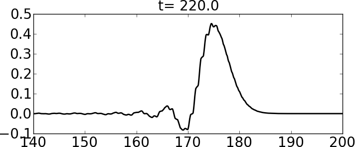
Figure 3: Transverse ($\theta=90^{\circ}$) linear wave propagation in a layered medium (5). The material coefficients are: (left) $c_{A}=1$, $c_{B}=4$ and $Z_{A}=Z_{B}=1$; (right) $c_{A}=c_{B}=1$, $Z_{A}=1$ and $Z_{B}=4$. The initial condition for both experiments is $\sigma({\bf x},t=0)=\exp(-x^{2}/10)$ and $u({\bf x},t=0)=v({\bf x},t=0)=0$.

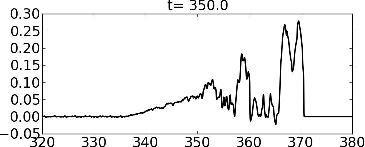
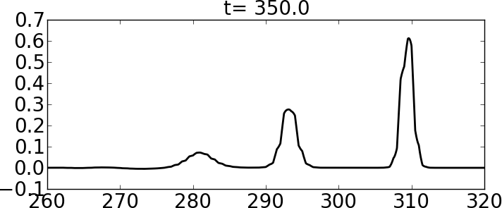
Figure 4: Transverse ($\theta=90^{\circ}$) nonlinear wave propagation in a layered medium (5). The material coefficients are: (left) $c_{A}=c_{B}=1$, $Z_{A}=1$ and $Z_{B}=1.5$; (right) $c_{A}=c_{B}=1$, $Z_{A}=1$ and $Z_{B}=4$. The initial condition for both experiments is $\sigma({\bf x},t=0)=\exp(-x^{2}/10)$ and $u({\bf x},t=0)=v({\bf x},t=0)=0$.

Up to this point we have considered dispersion induced by effective reflections at the material interfaces when the impedance varies. We refer to this effect as ‘$Z$-dispersion’ since it depends on variation in the impedance, which is commonly denoted by $Z$ in elasticity theory.

1.4 $C$-dispersion: effective dispersion induced by diffraction

In [28] the authors considered linear waves traveling in the same type of medium considered in the present work. Let us now review what was observed therein for parallel propagation; i.e. $\theta=0^{\circ}$ in Figure 1. In this case, if the sound speed differs in the $A$ and $B$ layers, effective dispersion is again introduced (even if the impedance is constant). We refer to this effect as ‘$C$-dispersion’ since it depends on variation in the sound speed, which is commonly denoted by $c$ in elasticity theory. In the nonlinear case, $C$-dispersion can also act as a regularization mechanism to delay or avoid the formation of shocks. If the dispersion is large, the nonlinear and the dispersive effects can balance each other, leading to the formation of solitary waves [15]. In Figure 5 we demonstrate this effect.

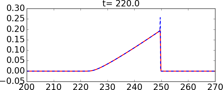
Figure 5: Parallel ($\theta=0^{\circ}$) nonlinear wave propagation in a layered medium (5). Sufficiently large variation in sound speed seems to prevent shock formation. The material coefficients are: (left) $c_{A}=1$, $c_{B}=1.1$ and $Z_{A}=Z_{B}=1$; (right) $c_{A}=1$, $c_{B}=4$ and $Z_{A}=Z_{B}=1$. We plot in solid red a slice through the middle of the $B$-layer and in dashed blue a slice through the middle of the $A$-layer. The initial condition for both experiments is $\sigma({\bf x},t=0)=\exp(-x^{2}/10)$ and $u({\bf x},t=0)=v({\bf x},t=0)=0$.

For general propagation along an arbitrary angle $\theta$, effective $Z$-dispersion and effective $C$-dispersion may both be introduced, due to variations in the impedance and the sound speed, respectively. The strength of each effect depends on the material parameters and the direction of propagation.

1.5 Shock speed

In this work we focus on a setting in which the dispersive effects are small (or the initial data is large), so that shocks may still appear. We are interested in the speed of propagation of the resulting shocks. This was studied in [16] for the case of transverse propagation (i.e., $\theta=90^{\circ}$ in Figure 1), in which case the problem is one-dimensional and there are only $Z$-dispersive effects. Following the notation therein, let $\sigma$, $\epsilon$ and $\rho$ denote stress, strain, and density, respectively. The hypothesized shock speed from [16] is then

$$s=\sqrt{\frac{1}{\rho_{m}}\left(\frac{[\sigma]}{[\epsilon]}\right)_{h}},$$ (9)

where $(\cdot)_{h}$ is the harmonic average operator (over one spatial period of the medium), $\rho_{m}$ is the mean density and $[z]=z_{r}-z_{l}$ denotes the jump in quantity $z$ across the shock. Formula (9) is just the usual Rankine-Hugoniot shock speed but with each quantity replaced by an appropriate spatial average. The choice to use an ordinary average for $\rho$ and a harmonic average for $\sigma/\epsilon$ is based on the fact that small-amplitude, long-wavelength pulses travel at an effective speed given by

$$c_{\text{eff}}=\sqrt{\frac{K_{h}}{\rho_{m}}},$$ (10)

where $K$ is the bulk-modulus; see [29]. Thus (9) is a natural extension of the Rankine-Hugoniot condition to determine the speed of shocks using effective material parameters. In Figure 6a we demonstrate the correctness of this estimate by considering a right going shock (as those we study in §3.1) propagating in a $Z$-dispersive medium with impedance in material A and B to be given by $Z_{A}=1$ and $Z_{B}=4$ respectively. The cyan dashed line represents the position of the shock as predicted by (9).

One might expect that, under the more general scenario in Figure 1, shocks would propagate with the same speed (9). However, one quickly finds that this is not the case. For example, in Figure 6b we consider propagation along $\theta=45^{\circ}$ in a medium with the same material properties as before. Again, we indicate the shock position predicted by (9) with a cyan dashed line. It is clear that the results in [16] do not apply for the more general framework that we study in this work. In Figure 6b we show with a dashed red line the position predicted by the theory developed in the present work. We propose an effective speed of propagation that is based on a leading order homogenized system.

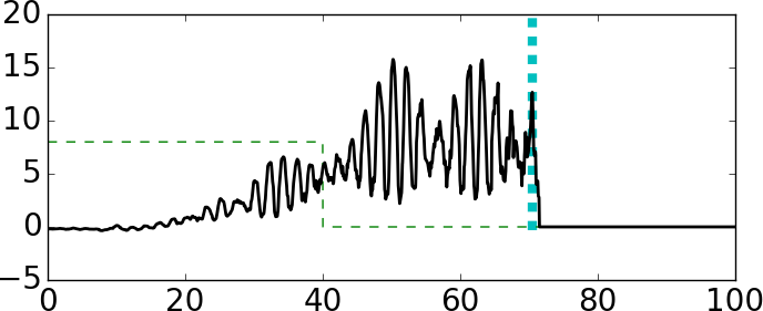
(a) Layered medium with $\theta=90^{\circ}$

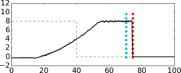
(b) Layered medium with $\theta=45^{\circ}$

Figure 6: Right-going shock in a layered medium (5) with (a) $\theta=90^{\circ}$ and (b) $\theta=45^{\circ}$. The material coefficients are $Z_{B}=1$, $Z_{A}=4$ and $c_{A}=c_{B}=1$. The initial condition is an effective purely right-going shock given by (28) with $x_{s}=40$, $u_{l}$ given by (27), $u_{r}=0$, $\sigma_{l}=8$ and $\sigma_{r}=0$. We show the solution at $t=20$ and use the nonlinear stress-strain relation (29a) In all plots, the black solid line is the solution along $y=0.5$, the cyan dashed line is the shock position predicted by (9) and the green dashed line is the initial condition. In (b), the red dashed line is the shock position predicted by our estimate (26), which we present in §3.

2 Homogenized equations

Our first goal is to generalize the proposed shock speed that was given in [16] for the case $\theta=90^{\circ}$. In order to do so, and also to place that hypothesis on a firmer mathematical footing, we perform an asymptotic analysis. Specifically, in this section we use homogenization theory to capture the macroscopic effects when waves with large wavelength travel in a periodic medium with small period $\Omega$ (relative to the wavelength). The leading-order result of this process is a constant-coefficient system with the material properties given by some average that depends on the relative angle between the propagation of the wave and the variation in the medium. We follow [15] and references therein. Recall system (3):

$$\epsilon_{t}-(u_{x}+v_{y}) =0,$$ (11a)

$$\rho u_{t}-\sigma_{x} =0,$$ (11b)

$$\rho v_{t}-\sigma_{y} =0.$$ (11c)

From §1.1 we have $\sigma_{\epsilon}=K({\bf x})G(\sigma)$. Using the chain rule, $\sigma_{t}=\sigma_{\epsilon}\epsilon_{t}$. Therefore, we can write (11) as

$$K^{-1}\sigma_{t}-G(\sigma)(u_{x}+v_{y}) =0,$$ (12a)

$$\rho u_{t}-\sigma_{x} =0,$$ (12b)

$$\rho v_{t}-\sigma_{y} =0.$$ (12c)

We start by introducing a parameter $\delta=\Omega/\lambda$, where $\Omega$ is the material period and $\lambda$ is the wave length. We restrict our attention to waves with $\lambda\gg\Omega\implies\delta\ll 1$. We recognize and introduce a fast spatial scale $\hat{\xi}=\delta^{-1}\xi$ where $\xi=x\sin\theta+y\cos\theta$ (is obtained by a simple rotation of axes and) defines the direction of the heterogeneity. We assume $\sigma=\sigma(x,y,\hat{\xi},t)$, $u=u(x,y,\hat{\xi},t)$ and $v=v(x,y,\hat{\xi},t)$ and that the material properties depend only on the fast scale; i.e., $\rho=\rho(\hat{\xi})$ and $K=K(\hat{\xi})$.

By the chain rule $\partial_{x}\mapsto\partial_{x}+\delta^{-1}\partial_{\hat{\xi}}\sin\theta$ and $\partial_{y}\mapsto\partial_{y}+\delta^{-1}\partial_{\hat{\xi}}\cos\theta$. Therefore (12) becomes

$$K^{-1}\sigma_{t}-G(\sigma)[u_{x}+v_{y}+\delta^{-1}(u_{\hat{\xi}}\sin\theta+v_{\hat{\xi}}\cos\theta)] =0,$$ (13a)

$$\rho u_{t}-(\sigma_{x}+\delta^{-1}\sigma_{\hat{\xi}}\sin\theta) =0,$$ (13b)

$$\rho v_{t}-(\sigma_{y}+\delta^{-1}\sigma_{\hat{\xi}}\cos\theta) =0.$$ (13c)

The next step is to expand $\sigma(x,y,\hat{\xi},t)$, $u(x,y,\hat{\xi},t)$ and $v(x,y,\hat{\xi},t)$ using the small parameter $\delta$. For example, $\sigma(x,y,\hat{\xi},t)=\sum_{i=0}^{\infty}\delta^{i}\sigma_{i}(x,y,\hat{\xi},t)$ and similarly for $u$ and $v$. We plug these expansions into (13) to get

$$K^{-1}\sum_{i=0}^{\infty}\delta^{i}\sigma_{i,t}-G\left(\sigma\right)\left(\sum_{i=0}^{\infty}\delta^{i}u_{i,x}+\sum_{i=0}^{\infty}\delta^{i}v_{i,y}+\sum_{i=0}^{\infty}\delta^{i-1}(u_{i,\hat{\xi}}\sin\theta+v_{i,\hat{\xi}}\cos\theta)\right) =\ 0,$$ (14a)

$$\rho\sum_{i=0}^{\infty}\delta^{i}u_{i,t}-\left(\sum_{i=0}^{\infty}\delta^{i}\sigma_{i,x}+\sum_{i=0}^{\infty}\delta^{i-1}\sigma_{i,\hat{\xi}}\sin\theta\right) =0,$$ (14b)

$$\rho\sum_{i=0}^{\infty}\delta^{i}v_{i,t}-\left(\sum_{i=0}^{\infty}\delta^{i}\sigma_{i,y}+\sum_{i=0}^{\infty}\delta^{i-1}\sigma_{i,\hat{\xi}}\cos\theta\right) =0,$$ (14c)

where $(\cdot)_{i,z}$ denotes differentiation of $(\cdot)_{i}$ with respect to $z$. The function $G(\sigma)$ is expanded around $\sigma_{0}$ using Taylor series as $G(\sigma)=G(\sigma_{0})+\delta G^{\prime}(\sigma_{0})\sigma_{1}+\dots$.

From (14), we collect the terms of order ${\mathcal{O}}(\delta^{-1})$:

$$(u_{0}\sin\theta+v_{0}\cos\theta)_{\hat{\xi}} =0,$$ (15a)

$$\sigma_{0,\hat{\xi}}\sin\theta =0,$$ (15b)

$$\sigma_{0,\hat{\xi}}\cos\theta =0,$$ (15c)

which implies that $\sigma_{0}=:\bar{\sigma}_{0}(x,y,t)$ and that $u_{0}\sin\theta+v_{0}\cos\theta$ is independent of $\hat{\xi}$. Here we use the notation that variables independent of the fast scale $\hat{\xi}$ are denoted by a bar.

From (14), we collect the terms of order ${\mathcal{O}}(\delta)$:

$$K^{-1}\bar{\sigma}_{0,t}-G(\bar{\sigma}_{0})\left(u_{0,x}+v_{0,y}+u_{1,\hat{\xi}}\sin\theta+v_{1,\hat{\xi}}\cos\theta\right) =0,$$ (16a)

$$\rho u_{0,t}-\left(\bar{\sigma}_{0,x}+\sigma_{1,\hat{\xi}}\sin\theta\right) =0,$$ (16b)

$$\rho v_{0,t}-\left(\bar{\sigma}_{0,y}+\sigma_{1,\hat{\xi}}\cos\theta\right) =0.$$ (16c)

Multiply equation (16b) by $\rho^{-1}$, apply the averaging operator

$$\left\langle\cdot\right\rangle:=\frac{1}{\Omega}\int_{0}^{\Omega}(\cdot)d\xi=\frac{1}{\lambda}\int_{0}^{\lambda}(\cdot)d\hat{\xi}$$ (17)

and multiply the resulting equation by $\cos\theta$. Similarly, multiply equation (16c) by $\rho^{-1}$, apply the averaging operator and multiply the resulting equation by $\sin\theta$. Combine the two equations to get

$$\left(\bar{u}_{0}\cos\theta-\bar{v}_{0}\sin\theta\right)_{t}-\rho_{h}^{-1}\left(\bar{\sigma}_{0,x}\cos\theta-\bar{\sigma}_{0,y}\sin\theta\right)=0,$$ (18)

where $\rho_{h}:=\left\langle\rho^{-1}\right\rangle^{-1}$ denotes the harmonic average. Here we defined $\bar{u}_{0}:=\left\langle u_{0}\right\rangle$ and $\bar{v}_{0}:=\left\langle v_{0}\right\rangle$. Multiply equation (16b) by $\sin\theta$ and equation (16c) by $\cos\theta$ and sum the two equations to obtain

$$\rho\left(u_{0}\sin\theta+v_{0}\cos\theta\right)_{t}-(\bar{\sigma}_{0,x}\sin\theta+\bar{\sigma}_{0,y}\cos\theta)-\sigma_{1,\hat{\xi}}=0.$$ (19)

Apply the averaging operator to (19) noting that by (15a) $u_{0}\sin\theta+v_{0}\cos\theta$ is independent of $\hat{\xi}$. Doing this yields

$$\left(\bar{u}_{0}\sin\theta+\bar{v}_{0}\cos\theta\right)_{t}-\rho_{m}^{-1}\left(\bar{\sigma}_{0,x}\sin\theta+\bar{\sigma}_{0,y}\cos\theta\right)=0,$$ (20)

where $\rho_{m}:=\left\langle\rho\right\rangle$ denotes the arithmetic average. Here we assumed $\sigma_{1,\hat{\xi}}$ is periodic with respect to the fast variable $\hat{\xi}$, which is a standard assumption in homogenization theory (see for instance [9, 3] and references therein). Multiply (18) by $\cos\theta$ and (20) by $\sin\theta$ and sum the two equations to obtain

$$\bar{u}_{0,t}-\left(\rho_{h}^{-1}\cos^{2}\theta+\rho_{m}^{-1}\sin^{2}\theta\right)\bar{\sigma}_{0,x}-\left(\rho_{m}^{-1}-\rho_{h}^{-1}\right)\sin\theta\cos\theta\bar{\sigma}_{0,y}=0.$$ (21)

Apply the averaging operator to (16a) (again assuming $\hat{\xi}$-periodicity of $u_{1,\hat{\xi}}$ and $v_{1,\hat{\xi}}$) to obtain

$$\overline{K}^{-1}\bar{\sigma}_{0,t}-G(\bar{\sigma}_{0})(\bar{u}_{0,x}+\bar{v}_{0,y}) =0.$$ (22)

Finally, for a plane wave propagating in the $x$-direction, we have $\bar{\sigma}_{0,y},\bar{v}_{0,y}=0$. Therefore,

$$\overline{K}^{-1}\bar{\sigma}_{0,t}-G(\bar{\sigma}_{0})\bar{u}_{0,x} =0,$$ (23a)

$$\overline{\rho}(\theta)\bar{u}_{0,t}-\bar{\sigma}_{0,x} =0,$$ (23b)

where $\overline{\rho}(\theta)=\left(\rho_{h}^{-1}\cos^{2}\theta+\rho_{m}^{-1}\sin^{2}\theta\right)^{-1}$ is the effective density in the oblique medium and $\overline{K}=\left\langle K^{-1}\right\rangle^{-1}$ is the effective bulk-modulus. Equations (23) constitute the leading order constant-coefficient homogenized system. We can now identify the effective material properties. The effective bulk-modulus is given by the harmonic average and the effective density is given by $\overline{\rho}(\theta)$. This agrees with the theory in [28] where the two cases $\theta=0^{\circ}$ and $\theta=90^{\circ}$ are considered.

3 Effective Rankine-Hugoniot conditions

The homogenized equations, which are given by (23), can be rewritten as a system of conservation laws:

$$\epsilon_{t}-u_{x} =0,$$ (24a)

$$\overline{\rho}(\theta)u_{t}-\overline{\sigma}_{x} =0.$$ (24b)

The system (24) is closed by choosing a nonlinear stress-strain relation $\overline{\sigma}(\epsilon)=\sigma(\epsilon;\overline{K})$. This leading order system is a dispersionless approximation of the original problem; i.e., it captures the effective behavior of the solution neglecting the dispersive effects. Therefore, it yields a better approximation when the dispersion is small. In this work we are interested in the case when (viscous) shocks form which is expected to happen when the effective dispersion is small. In this regime, it is reasonable to expect the shock to propagate with speed close to that given by applying the Rankine-Hugoniot conditions to (24). By doing this we obtain

$$s[\epsilon] =-[u],$$ (25a)

$$\overline{\rho}(\theta)s[u] =-[\overline{\sigma}],$$ (25b)

where $s$ is the speed of the shock and $[(\cdot)]$ is the jump of $(\cdot)$; i.e., $[(\cdot)]:=(\cdot)_{l}-(\cdot)_{r}$. Therefore, we propose an estimate for the speed of propagation of viscous shocks to be given by

$$s_{\text{eff}}=\pm\sqrt{\frac{[\overline{\sigma}]}{\overline{\rho}(\theta)[\epsilon]}},$$ (26)

where the minus and plus sign correspond to the left- and right-going shocks, respectively. Note that $\overline{\rho}(\theta)$ increases as $\theta$ gets closer to $90^{\circ}$. Therefore, the speed of the shock is reduced as $\theta$ gets closer to $90^{\circ}$. A similar result for long-wavelength linear waves is well known; see e.g. [25, 1].

3.1 Effective purely right-going shocks

The Rankine-Hugoniot conditions not only provide the speed of propagation of shocks but also the proper way to connect left and right states of a shock. Without loss of generality we consider just right-going shocks, which correspond to the positive speed $s_{\text{eff}}$ in (26). From (25), we get

$$[u]=-\sqrt{\frac{[\overline{\sigma}][\epsilon]}{\overline{\rho}(\theta)}}.$$ (27)

This expression provides the connection between the left and right state for a right-going shock. We perform experiments on different layered media with coefficients given by (5). In these experiments the nonlinear constitutive relation $\overline{\sigma}(\epsilon)$ is given by (29a) with $K=\overline{K}$, and the initial condition is

$$\sigma({\bf x},t=0)=\begin{cases}\sigma_{l},&\text{ if }x\leq x_{s}\\ \sigma_{r},&\text{ if }x>x_{s}\end{cases}, u({\bf x},t=0)=\begin{cases}u_{l},&\text{ if }x\leq x_{s}\\ u_{r},&\text{ if }x>x_{s}\end{cases}, v({\bf x},t=0)=0,$$ (28)

where $x_{s}$ defines the position of the shock, $u_{l}$ is given by (27), $\sigma_{l}=1$, $\sigma_{r}=0$ and $u_{r}=0$. For all the experiments, we solve the original variable coefficient system (1) and the leading order homogenized system (24). We consider two stress relations:

$$\sigma(\epsilon,{\bf x}) =\exp(K({\bf x})\epsilon)-1,$$ (29a)

$$\sigma(\epsilon,{\bf x}) =\alpha K({\bf x})\epsilon+\beta(K({\bf x})\epsilon)^{2}+\gamma(K({\bf x})\epsilon)^{3},$$ (29b)

with $\alpha,\beta,\gamma\in\mathbb{R}$. Both are smooth, one-to-one functions; the first has been used before in [20] while the second is important in nonlinear optics [2]. We take $\alpha=0.1,\beta=0$ and $\gamma=5$.

We first consider parallel propagation ($\theta=0^{\circ}$ in Figure 1). In this case $C$-dispersion is introduced by diffraction due to variation in the sound speed. Results are shown in Figure 7 for media with sound speed contrast of $c_{B}/c_{A}=4,\leavevmode\nobreak\ 2,\leavevmode\nobreak\ 1.25,\mbox{ and }1$. When $c_{B}/c_{A}=1$ we use $K_{A}=\rho_{A}=1$ and $K_{B}=\rho_{B}=4$; i.e., the medium is still non-homogeneous. For all other cases we use

$$K_{A} =\frac{1+c_{B}/c_{A}}{2c_{B}/c_{A}}, \qquad\rho_{A} =\frac{1}{K_{A}},$$ (30a)

$$K_{B} =\frac{1+c_{B}/c_{A}}{2}, \qquad\rho_{B} =\frac{1}{K_{B}}.$$ (30b)

In the last three cases the approximation is very good. In the first case, a train of solitons forms and no singular shock is discernible. Clearly, the approximation is better when the sound speed contrast is small. For the last two plots, we show a zoomed image of the region near the shock. Note that the effect of dispersion is still evident when $c_{B}/c_{A}=1.25$, which is not the case when $c_{B}/c_{A}=1$.

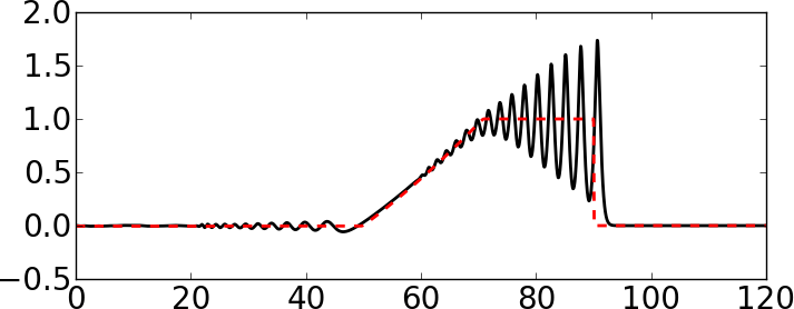
\begin{overpic}[scale={0.175}]{figures/right-going_c-dispersive_r1-25.png} \put(52.5,28.0){\includegraphics[scale={0.15}]{figures/cBcA_ratio_1p25.png}} \end{overpic}

\begin{overpic}[scale={0.175}]{figures/right-going_c-dispersive_r1.png} \put(52.5,28.0){\includegraphics[scale={0.15}]{figures/cBcA_ratio_1.png}} \end{overpic}

Figure 7: Effective right-going shocks in a layered medium with $\theta=0^{\circ}$. The material coefficients are given by (5) with sound speed contrast of (from left to right) $c_{B}/c_{A}=4,\leavevmode\nobreak\ 2,\leavevmode\nobreak\ 1.25$ and $1$. When $c_{B}/c_{A}=1$ we use $K_{A}=\rho_{A}=1$ and $K_{B}=\rho_{B}=4$. For all other cases we use (30). The red dashed line is the solution of the homogenized system (23). The initial condition is an effective purely right-going shock given by (28) with $x_{s}=30$, $u_{l}$ given by (27), $u_{r}=0$, $\sigma_{l}=1$ and $\sigma_{r}=0$. We show the solution at $t=40$ and use the nonlinear stress-strain relation (29a). For the last two plots, we show an enlarged view of the region near the shock.

For $\theta\in(0^{\circ},90^{\circ})$, both $C$- and $Z$-dispersion are introduced by diffraction and reflections due to variation in the sound speed and impedance, respectively. In Figure 8 we consider $\theta=22.5^{\circ},\leavevmode\nobreak\ 45^{\circ}$ and $67.5^{\circ}$ and media with different sound speed and impedance contrast. We use $c_{B}/c_{A}=Z_{B}/Z_{A}=4,\leavevmode\nobreak\ 2$ and $1.25$ (with $c_{A}=1$ and $Z_{A}=1$). Again, the approximation improves as the sound speed and impedance contrasts are reduced.

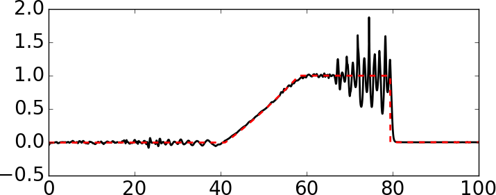
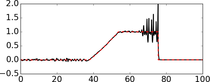
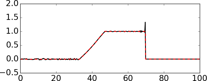
(a) $\theta=22.5^{\circ}$

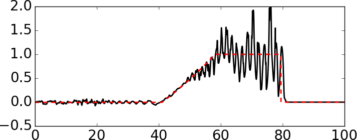
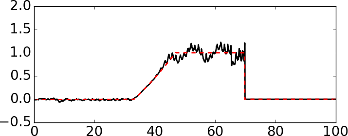
(b) $\theta=45^{\circ}$

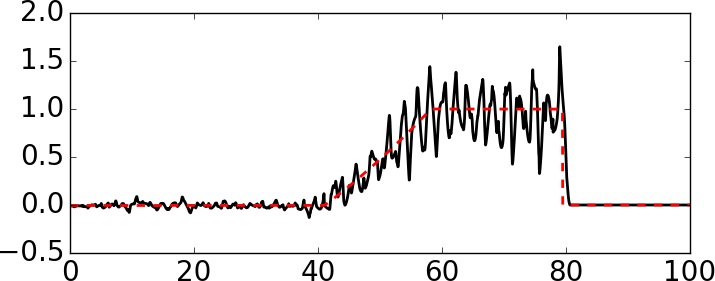
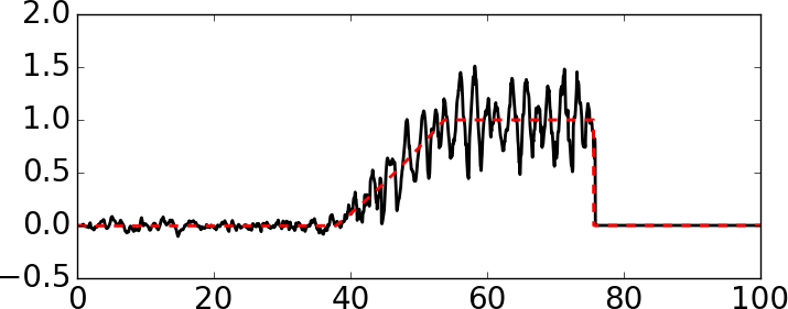
(c) $\theta=67.5^{\circ}$

Figure 8: Effective right-going shock in a layered medium with (a) $\theta=22.5^{\circ}$, (b) $\theta=45^{\circ}$ and (c) $\theta=67.5^{\circ}$. The material coefficients are given by (5) with impedance and sound speed contrast of (from left to right) $Z_{B}/Z_{A}=c_{B}/c_{A}=4,\leavevmode\nobreak\ 2$ and $1.25$ (with $c_{A}=1$ and $Z_{A}=1$). The red dashed line is the solution of the homogenized system (23). The initial condition is an effective purely right-going shock given by (28) with $x_{s}=30$, $u_{l}$ given by (27), $u_{r}=0$, $\sigma_{l}=1$ and $\sigma_{r}=0$. We show the solution at $t=30$ and use the nonlinear stress-strain relation (29a).

Finally, when $\theta=90^{\circ}$ $Z$-dispersion is introduced by reflections due to variation in the impedance. We consider media with impedance contrast of $Z_{B}/Z_{A}=4,\leavevmode\nobreak\ 2,\leavevmode\nobreak\ 1.25$ and $1$. The results are shown in Figure 9. When $Z_{B}/Z_{A}=1$ the material parameters are given by $K_{A}=\rho_{A}=1$, $K_{B}=4$ and $\rho_{B}=1/4$; i.e., the material is still non-homogeneous. For all other cases we use $K_{A}=\rho_{A}=1$ and $K_{B}=\rho_{B}=Z_{B}/Z_{A}$. As before, the leading order approximation improves as the impedance contrast is reduced.

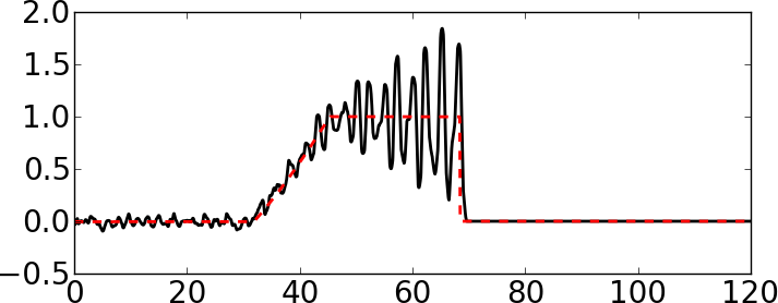
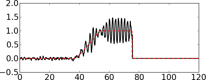
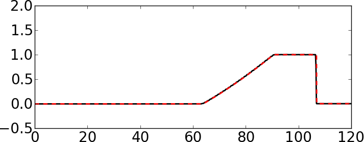
Figure 9: Effective right-going shock in a layered medium with $\theta=90^{\circ}$. The material coefficients are given by (5) with impedance contrast of (from left to right) $Z_{B}/Z_{A}=4,\leavevmode\nobreak\ 2,\leavevmode\nobreak\ 1.25$ and $1$. When $Z_{B}/Z_{A}=1$ we use $K_{A}=\rho_{A}=1$, $K_{B}=4$ and $\rho_{B}=1/4$. For all other cases we use $K_{A}=\rho_{A}=1$ and $K_{B}=\rho_{B}=Z_{B}/Z_{A}$. The red dashed line is the solution of the homogenized system (23). The initial condition is an effective purely right-going shock given by (28) with $x_{s}=30$, $u_{l}$ given by (27), $u_{r}=0$, $\sigma_{l}=1$ and $\sigma_{r}=0$. We show the solution at $t=40$ and use the nonlinear stress-strain relation (29a).

Evidently, the microscopic effects of the induced dispersion (i.e, the oscillatory behavior) cannot be described by the homogenized system (23). This is expected since it is only a leading order approximation. Indeed, one of the assumptions during the homogenization process is that the wavelength of the pulse is large compared to the periodicity in the medium, which is not the case for the right-going shock in these experiments. Nevertheless, the homogenized system seems to accurately predict not only the speed of the shock but also the macroscopic behavior of the solution.

Remark 3.1.1 (Numerical methods).

We solve the variable-coefficient system (1) and the homogenized system (23) using PyClaw [14]. Within PyClaw, we use the classic algorithm implemented in Clawpack [35], which is a second order method in space and time based on a Lax-Wendroff discretization combined with Total Variation Diminishing (TVD) limiters. This algorithm is a finite volume method for solving hyperbolic conservation laws based on the (approximate) solution of Riemann problems. The Riemann solvers can be found in [27]. The resolution in all the experiments in this work is characterized by a mesh size of $\Delta x=\Delta y=1/128$.

3.2 Effective shock-speed

In this section we perform (a total of 1620) numerical simulations to corroborate the estimate (26), which predicts the speed of propagation of shocks in periodic media. The experiments are split into four cases. For cases (a) and (b) we use a layered medium (5) with exponential (29a) and cubic (29b) nonlinearities, respectively; for cases and (c) and (d) we use a sinusoidal medium (4) with exponential (29a) and cubic (29b) nonlinearities, respectively. For each of these four cases, we consider $\theta\in\{0^{\circ},22.5^{\circ},45^{\circ},67.5^{\circ},90^{\circ}\}$. For each value of $\theta$, we perform 81 experiments all starting with a right-going shock given by (28) with $u_{l}$ given by (27), $u_{r}=0$, $K_{A}=\rho_{A}=1$ and all possible combinations of:

$$\rho_{B} =\{2,\leavevmode\nobreak\ 3.5,\leavevmode\nobreak\ 5\}, K_{B} =\{2,\leavevmode\nobreak\ 3.5,\leavevmode\nobreak\ 5\},$$ (31a)

$$\sigma_{l} =\{2,\leavevmode\nobreak\ 4,\leavevmode\nobreak\ 8\}, \sigma_{r} =\{0,\leavevmode\nobreak\ 0.5,\leavevmode\nobreak\ 1\}.$$ (31b)

For each experiment, we measure the speed of the shock and compare it with the speed predicted by (26). Each experiment is represented by a dot in Figure 10, while the predicted speed is indicated by the red dashed line. The color of the dot represents the amount of dispersion introduced by the medium; darker colors correspond to less dispersive media as predicted by [28, equation (34)].

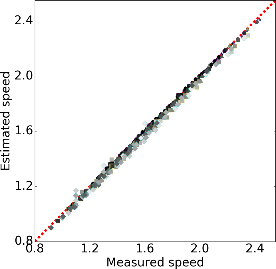
(a) Layered medium (5) with exp. nonlinearity (29a)

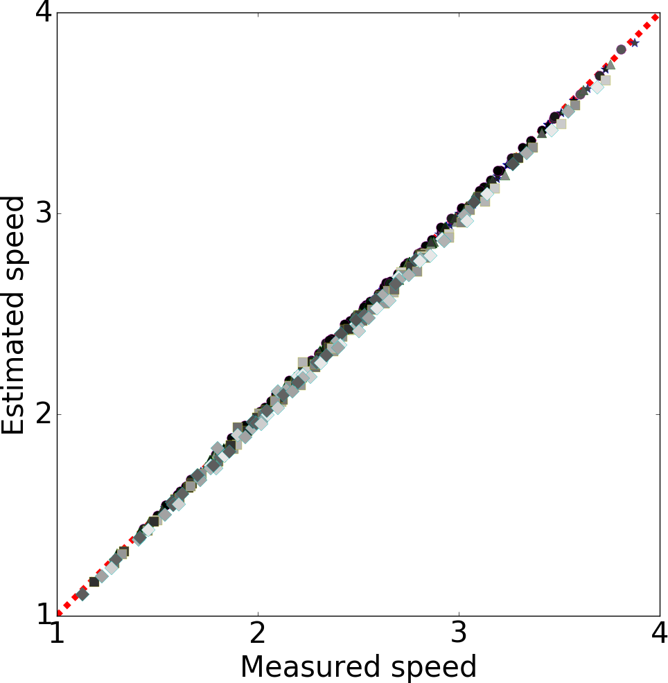
(b) Layered medium (5) with cubic nonlinearity (29b)

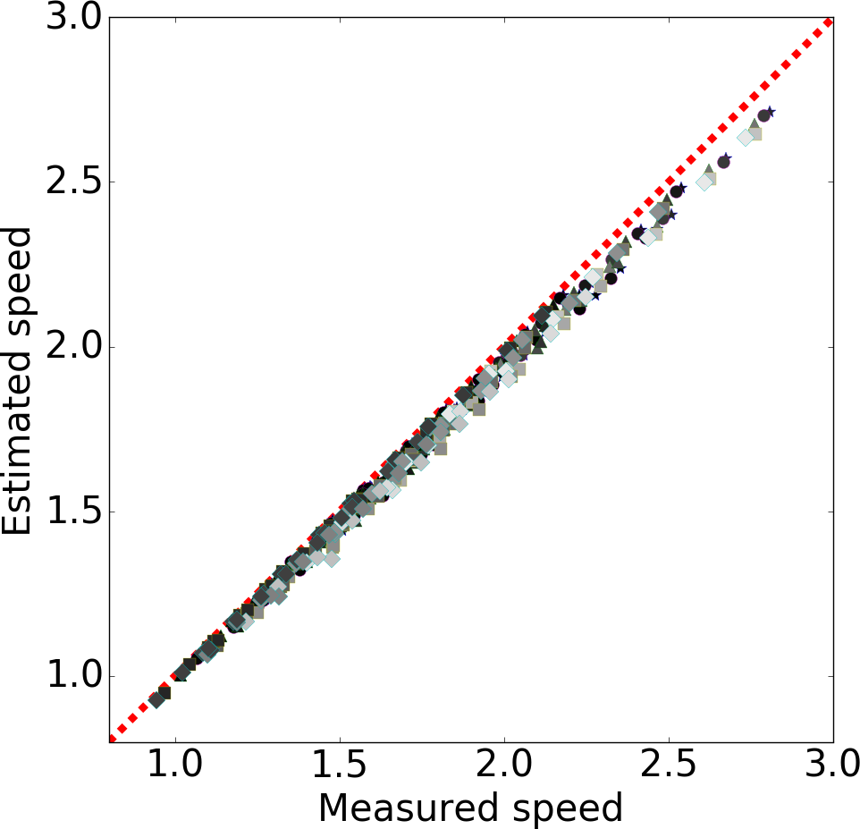
(c) Sinusoidal medium (4) with exp. nonlinearity (29a)

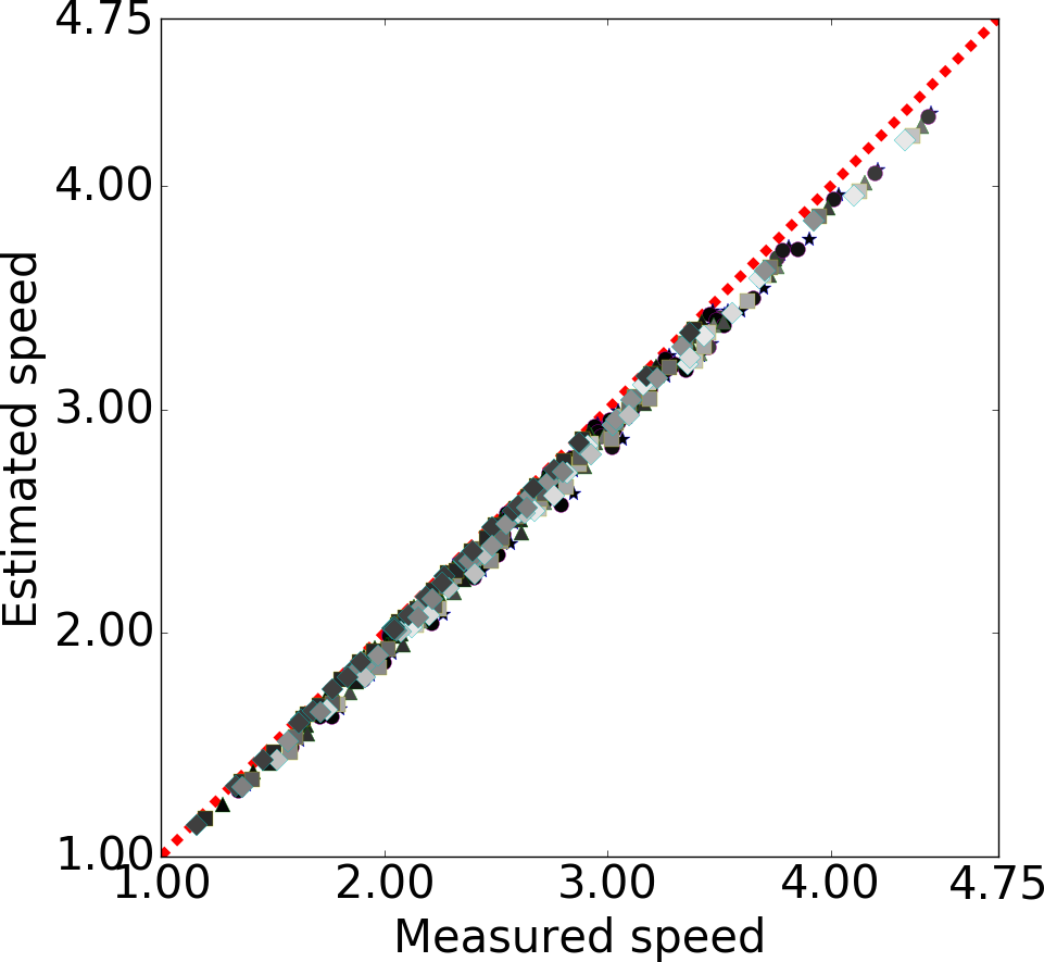
(d) Sinusoidal medium (4) with cubic nonlinearity (29b)

Figure 10: Estimated versus measured speed for 1620 experiments. We consider $\theta\in\{0^{\circ},22.5^{\circ},45^{\circ},67.5^{\circ},90^{\circ}\}$. The initial condition is an effective purely right-going shock given by (28) with $x_{s}=40$, $u_{l}$ given by (27), $u_{r}=0$, $K_{A}=\rho_{A}=1$ and all possible combinations of (31). Darker colors in the markers correspond to less dispersive media as predicted by [28, equation (34)].

4 Towards an effective Lax-entropy condition for periodic media

Consider the one-dimensional version of (1) written as a conservation law and consider only the nonlinear convex stress-strain relation (29a). A right-going shock for such system satisfies the Lax-entropy condition [18] if its speed, denoted as $s^{+}$, satisfies

$$\lambda^{+}_{l}>s^{+}>\lambda^{+}_{r},$$ (32)

which imposes that the right-going characteristics (denoted by $\lambda^{+}$) from the left and right state of the shock impinge each other. For a homogeneous medium, this condition is solely dependent upon the solution to the left and right of the shock.

In principle, it is reasonable to expect that the effective dispersion introduced in periodic media might regularize weak shocks that can otherwise propagate in homogeneous media. Therefore, it is desirable to identify a condition for a shock to be able to propagate as a stable shock in periodic media. This problem is studied in [16] for $Z$-dispersive media (i.e., media as in Figure 1 with $\theta=90^{\circ}$). The authors hypothesize that the speed $s_{\text{eff}}$ of a stable (right-going) shock must satisfy

$$s_{\text{eff}}>c_{h}(\sigma_{r}):=\left(\int_{0}^{1}\left(\frac{\sigma_{r}^{\prime}(x)}{\rho(x)}\right)^{-1/2}dx\right)^{-1}.$$ (33)

In other words, a stable right-going shock in a $Z$-dispersive medium must travel faster than the harmonic average of the sound speed. To corroborate this hypothesis, the authors perform multiple experiments monitoring the evolution of the (global) entropy

$$\eta(t)=\int_{\Omega}\left[\frac{1}{2}\rho(x)u^{2}+\int_{0}^{\epsilon}\sigma(z,x)dz\right]dx,$$ (34)

which remains constant for smooth solutions but decreases in the presence of shocks. This hypothesis, however, does not seem to accurately predict behavior in the more general situation depicted in Figure 1. We illustrate this in Figure 11, where we plot the evolution of the normalized entropy $\eta(t)/\eta(0)$ for different experiments. We consider $\theta\in\{0^{\circ},\leavevmode\nobreak\ 90^{\circ}\}$ and $K_{A}=\rho_{A}=\rho_{B}=1$, $K_{B}=16$. Note that $Z_{B}/Z_{A}=c_{B}/c_{A}=4$; i.e, both the impedance and the sound speed change in space. For each angle $\theta$, the initial condition is an effective purely right-going shock given by (28) with $x_{s}=15$, $u_{l}$ given by (27), $u_{r}=0$, $\sigma_{r}=0$ and $\sigma_{l}$ chosen so that (using (26)) $s_{\text{eff}}/c_{h}(\sigma_{r})=\{0.95,\leavevmode\nobreak\ 0.975,\leavevmode\nobreak\ 1.025,\leavevmode\nobreak\ 1.05\}$. When $\theta=90^{\circ}$ (the situation studied in [16]), shocks with speed $s_{\text{eff}}>c_{h}(\sigma_{r})$ propagate as stable viscous shocks (i.e., do not get regularized). Otherwise, the shock is regularized by the induced dispersion and the entropy remains constant. Note that some entropy is lost in all simulations due to numerical dissipation. The condition (33) clearly does not hold for $\theta=0^{\circ}$.

(a) $C$-dispersive media ($\theta=0^{\circ}$)

(b) $Z$-dispersive media ($\theta=90^{\circ}$)

Figure 11: Normalized entropy evolution for two different media with $\theta=\{0^{\circ},\leavevmode\nobreak\ 90^{\circ}\}$. The material coefficients are given by the layered medium (5) with $K_{A}=\rho_{A}=\rho_{B}=1$ and $K_{B}=16$ $\implies Z_{B}/Z_{A}=c_{B}/c_{A}=4$. The initial condition is an effective purely right-going shock given by (28) with $x_{s}=15$, $u_{l}$ given by (27), $u_{r}=0$, $\sigma_{r}=0$ and $\sigma_{l}$ chosen so that (using (26)) $s_{\text{eff}}/c_{h}(\sigma_{r})=\{0.95,\leavevmode\nobreak\ 0.975,\leavevmode\nobreak\ 1.025,\leavevmode\nobreak\ 1.05\}$.

We found empirically that for $C$-dispersive media with $Z=1$, the speed of a stable (right-going) shock satisfies

$$s_{\text{eff}}>c_{m}(\sigma_{r}):=\int_{0}^{1}\frac{\sigma_{r}^{\prime}(x)}{\rho(x)}dx.$$ (35)

We illustrate this in Figure 12, where we perform multiple experiments all with the material parameters given by $K_{A}=\rho_{A}=1$, $K_{B}=4$ and $\rho_{B}=1/4$ $\implies Z_{A}=Z_{B}=1,\leavevmode\nobreak\ c_{B}/c_{A}=4$. In all the experiments the initial condition is an effective purely right-going shock given by (28) with $x_{s}=15$, $u_{l}$ given by (27), $u_{r}=0$, $\sigma_{r}=0$ and $\sigma_{l}$ chosen so that (using (26)) $s_{\text{eff}}/c_{m}(\sigma_{r})\in[0.8,\leavevmode\nobreak\ 1.6]$. We measure the entropy lost at $t=20$, which is significant when $s_{\text{eff}}>c_{m}(\sigma_{r})$. This indicates that viscous shocks remain stable through the entire simulation; otherwise, the shocks are regularized and the entropy is roughly constant (up to numerical errors). We consider different mesh widths to demonstrate the effect of numerical dissipation in the entropy lost.

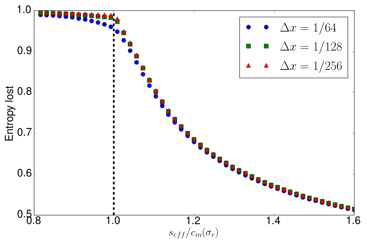
Figure 12: Entropy lost at $t=20$ in $C$-dispersive media with $Z=1$. The material coefficients are given by the layered medium (5) with $K_{A}=\rho_{A}=1$, $K_{B}=4$ and $\rho_{B}=1/4$ $\implies Z=1,\leavevmode\nobreak\ c_{B}/c_{A}=4$. The initial condition is an effective purely right-going shock given by (28) with $x_{s}=15$, $u_{l}$ given by (27), $u_{r}=0$, $\sigma_{r}=0$ and $\sigma_{l}$ chosen so that (using (26)) $s_{\text{eff}}/c_{m}(\sigma_{r})\in[0.8,\leavevmode\nobreak\ 1.6]$.

By performing experiments (not shown here) in more general media (i.e., with $Z\neq 1$) we conclude that condition (35) does not hold in general. We are interested in a generalized Lax-entropy condition for periodic media (like the one depicted in Figure 1); however, for now that problem remains open. In §5 we discuss potential alternatives to solve this problem.

5 Conclusions

Since a shock (or any wave) that propagates in a periodic medium may be influenced by effective dispersion, it is important to make the distinction between viscous shocks and dispersive shocks. Viscous shocks are characterized by the presence of (nearly) discontinuous fronts and by loss in entropy (which in this work is defined by (34)). The main result of this work is an estimate for the speed of a vanishing-viscosity shock propagating in a periodic medium, based on a leading order – dispersionless – homogenized system. Through multiple numerical experiments, we tested the validity of this estimate and found that the agreement is good. Nevertheless, it is important to remark that the estimate is expected to hold only when the dispersive effects are relatively small. These results represent a generalization of the results presented in [16].

We are also interested in finding a condition for a shock to propagate in periodic media without being regularized by the induced dispersive effects. Such a condition has been developed in [16] for the one-dimensional setting. Although in experiments we have observed similar trend (namely, that larger shocks in less-dispersive media tend to persist), we have not found an extension of the specific criterion from [16] to the 2D medium considered here. We found empirically that when $\theta=0^{\circ}$ and $Z=1$ stable (right-going) shocks propagate with speed such that $s_{\text{eff}}>c_{m}(\sigma_{r})$ where $c_{m}(\sigma_{r})$ denotes the mean value of the sound speed (to the right of the shock) in the periodic medium. Nevertheless, this condition does not hold for more general media. A general condition might be found by deriving a dispersive correction to the leading order homogenized system (23) (like the ones obtained in [20, 9, 15]) and then applying a relaxation method (like in [23, 8]) that would allow writing the dispersive homogenized system as a hyperbolic model. In such a model, the characteristic speeds would be modified by the dispersive effects via the relaxation term. Given such a hyperbolic model one could apply the standard theory of hyperbolic equations to obtain the Lax-entropy condition. One could also study this problem by deriving the dispersive homogenized system and then applying the modulation theory of [36].

References

- [1] George E Backus. Long-wave elastic anisotropy produced by horizontal layering. Journal of Geophysical Research, 67(11):4427–4440, 1962.
- [2] Robert W Boyd. Nonlinear optics. Elsevier, 2003.
- [3] Wen Chen and Jacob Fish. A dispersive model for wave propagation in periodic heterogeneous media based on homogenization with multiple spatial and temporal scales. Journal of applied mechanics, 68(2):153–161, 2001.
- [4] Carlos Conca and Muthusamy Vanninathan. Homogenization of periodic structures via Bloch decomposition. SIAM Journal on Applied Mathematics, 57(6):1639–1659, 1997.
- [5] AG Davies and AD Heathershaw. Surface-wave propagation over sinusoidally varying topography. Journal of Fluid Mechanics, 144:419–443, 1984.
- [6] GA El and MA Hoefer. Dispersive shock waves and modulation theory. Physica D: Nonlinear Phenomena, 333:11–65, 2016.
- [7] Chris L Farmer, Hilary Ockendon, and John R Ockendon. Wave propagation along periodic layers. SIAM Journal on Applied Mathematics, 78(4):2154–2175, 2018.
- [8] N Favrie and S Gavrilyuk. A rapid numerical method for solving Serre–Green–Naghdi equations describing long free surface gravity waves. Nonlinearity, 30(7):2718, 2017.
- [9] Jacob Fish and Wen Chen. Higher-order homogenization of initial/boundary-value problem. Journal of Engineering Mechanics, 127(12):1223–1230, 2001.
- [10] Jean-Pierre Fouque, Josselin Garnier, and André Nachbin. Shock structure due to stochastic forcing and the time reversal of nonlinear waves. Physica D: Nonlinear Phenomena, 195(3-4):324–346, 2004.
- [11] Josselin Garnier, Juan Carlos Munoz Grajales, and André Nachbin. Effective behavior of solitary waves over random topography. Multiscale Modeling & Simulation, 6(3):995–1025, 2007.
- [12] P Halevi, AA Krokhin, and J Arriaga. Photonic crystal optics and homogenization of 2D periodic composites. Physical Review Letters, 82(4):719, 1999.
- [13] Vladimir Iosifovich Karpman. Non-Linear Waves in Dispersive Media: International Series of Monographs in Natural Philosophy, volume 71. Elsevier, 2016.
- [14] David I. Ketcheson, Kyle T. Mandli, Aron J. Ahmadia, Amal Alghamdi, Manuel Quezada de Luna, Matteo Parsani, Matthew G. Knepley, and Matthew Emmett. PyClaw: Accessible, Extensible, Scalable Tools for Wave Propagation Problems. SIAM Journal on Scientific Computing, 34(4):C210–C231, November 2012.
- [15] David I Ketcheson and Manuel Quezada de Luna. Diffractons: solitary waves created by diffraction in periodic media. Multiscale Modeling & Simulation, 13(1):440–458, 2015.
- [16] D.I. Ketcheson and R.J. LeVeque. Shock dynamics in layered periodic media. Communications in Mathematical Sciences, 10(3):859–874, 2012.
- [17] Manvir S Kushwaha, Peter Halevi, Leonard Dobrzynski, and Bahram Djafari-Rouhani. Acoustic band structure of periodic elastic composites. Physical Review Letters, 71(13):2022, 1993.
- [18] Peter D Lax. Hyperbolic systems of conservation laws and the mathematical theory of shock waves. SIAM, 1973.
- [19] Randall J. LeVeque. Finite volume methods for hyperbolic problems. Cambridge University Press, Cambridge, 2002.
- [20] Randall J. LeVeque and Darryl H. Yong. Solitary waves in layered nonlinear media. SIAM Journal on Applied Mathematics, 63:1539–1560, 2003.
- [21] Tai-Ping Liu. Decay to N-waves of solutions of general systems of nonlinear hyperbolic conservation laws. Communications on Pure and Applied Mathematics, 30(5):585–610, 1977.
- [22] Tai-Ping Liu. Linear and nonlinear large-time behavior of solutions of general systems of hyperbolic conservation laws. Communications on Pure and Applied Mathematics, 30(6):767–796, 1977.
- [23] Alireza Mazaheri, Mario Ricchiuto, and Hiroaki Nishikawa. A first-order hyperbolic system approach for dispersion. J. Comput. Physics, 321:593–605, 2016.
- [24] Yan Pennec, Jérôme O Vasseur, Bahram Djafari-Rouhani, Leonard Dobrzyński, and Pierre A Deymier. Two-dimensional phononic crystals: Examples and applications. Surface Science Reports, 65(8):229–291, 2010.
- [25] GW Postma. Wave propagation in a stratified medium. Geophysics, 20(4):780–806, 1955.
- [26] Peng Qu and Zhouping Xin. Long time existence of entropy solutions to the one-dimensional non-isentropic Euler equations with periodic initial data. Archive for Rational Mechanics and Analysis, 216(1):221–259, 2015.
- [27] Manuel Quezada de Luna and David I. Ketcheson. Numerical simulation of cylindrical solitary waves in periodic media. Journal of Scientific Computing, 58(3):672–689, 2014.
- [28] Manuel Quezada de Luna and David I Ketcheson. Two-dimensional wave propagation in layered periodic media. SIAM Journal on Applied Mathematics, 74(6):1852–1869, 2014.
- [29] F. Santosa and W. Symes. A dispersive effective medium for wave propagation in periodic composites. SIAM Journal on Applied Mathematics, 51:984–1005, 1991.
- [30] Michael Shefter and Rodolfo R Rosales. Quasiperiodic solutions in weakly nonlinear gas dynamics. Part I. Numerical results in the inviscid case. Studies in Applied Mathematics, 103(4):279–337, 1999.
- [31] K Solna and G Papanicolaou. Ray theory for a locally layered random medium. Waves in Random Media, 10(1):151, 2000.
- [32] C-T Sun, Jan D Achenbach, and George Herrmann. Continuum theory for a laminated medium. 1968.
- [33] C-T Sun, Jan Drewes Achenbach, and G Herrmann. Time-harmonic waves in a stratified medium propagating in the direction of the layering. Journal of Applied Mechanics, 35(2):408–411, 1968.
- [34] Yunfei Tang, Yifeng Shen, Jiong Yang, Xiaohan Liu, Jian Zi, and Xinhua Hu. Omnidirectional total reflection for liquid surface waves propagating over a bottom with one-dimensional periodic undulations. Physical Review E, 73(3):035302, 2006.
- [35] Clawpack Development Team. Clawpack software, 2013. Version 5.5.0.
- [36] Gerald Beresford Whitham. Non-linear dispersive waves. Proceedings of the Royal Society of London. Series A. Mathematical and Physical Sciences, 283(1393):238–261, 1965.
- [37] Darryl H. Yong and J. Kevorkian. Solving Boundary-Value Problems for Systems of Hyperbolic Conservation Laws with Rapidly Varying Coefficients. Studies in Applied Mathematics, 108(3):259–303, 2002.
- [38] Norman J Zabusky and Martin D Kruskal. Interaction of “solitons” in a collisionless plasma and the recurrence of initial states. Physical Review Letters, 15(6):240, 1965.