New bounds on the vertical heat transport for Bénard–Marangoni convection at infinite Prandtl number

Abstract

We prove a new rigorous upper bound on the vertical heat transport for Bénard–Marangoni  convection of a two- or three-dimensional fluid layer with infinite Prandtl number. Precisely, for Marangoni number $\mbox{\it Ma}\gg 1$ the Nusselt number Nu is bounded asymptotically by $\mbox{\it Nu}\leq\text{const.}\times\mbox{\it Ma}^{2/7}(\ln\mbox{\it Ma})^{-1/7}$. Key to our proof are a background temperature field with a hyperbolic profile near the fluid’s surface and new estimates for the coupling between temperature and vertical velocity.

1 Introduction

When a layer of fluid heated from below is subject to temperature gradients along its surface, local variations in the surface tension generate a shear stress. This phenomenon, called the Marangoni effect, can set the fluid in motion when the ratio of surface tension forces to viscosity is sufficiently large. The ensuing flow, known as Bénard–Marangoni  convection, can produce beautiful surface patterns as famously observed by H. Bénard (1901), and is a paradigm for pattern formation. It also underpins a number of industrial processes, such as fusion welding (DebRoy & David, 1995) and the growth of semiconductors (Lappa, 2010). Nevertheless, Bénard–Marangoni  convection remains poorly understood especially when compared to its buoyancy-driven counterpart, Rayleigh–Bénard convection.

A fundamental open problem is to determine the vertical heat transport as a function of the thermal forcing and the material parameters of the fluid. In nondimensional terms, one is interested in how the Nusselt number Nu varies with the Marangoni number Ma, which measures the relative strength of thermally-driven surface tension to viscous forces, and the Prandtl number Pr, given by the ratio between the kinematic viscosity and the thermal diffusivity of the fluid.

For finite Prandtl numbers, a phenomenological argument by Pumir & Blumenfeld (1996) predicts $\mbox{\it Nu}\sim\mbox{\it Ma}^{\frac{1}{3}}$ with a Prandtl-dependent prefactor when $\mbox{\it Ma}\gg 1$ and the flow is turbulent. Two-dimensional direct numerical simulations (DNS) with stress-free boundaries at low Pr support this scaling (Boeck & Thess, 1998), but no-slip boundaries in either two or three dimensions yield smaller powers of Ma (Boeck, 2005). Two-dimensional free-slip DNS at both high and infinite Pr also suggest a smaller exponent. Assuming steady convection rolls are stable at arbitrarily large Ma, a boundary-layer scaling analysis predicts $\mbox{\it Nu}\sim\mbox{\it Ma}^{\frac{2}{9}}$ in the infinite-Pr limit (Boeck & Thess, 2001).

Rigorous results, derived directly from the governing equations without introducing unproven assumptions, are key to substantiate or rule out any of these heuristic scaling arguments. By expressing the temperature field in terms of fluctuations around a carefully chosen steady “background” temperature field, Hagstrom & Doering (2010) proved that $\mbox{\it Nu}\lesssim\mbox{\it Ma}^{\frac{1}{2}}$ uniformly in Pr when this is finite, and $\mbox{\it Nu}\lesssim\mbox{\it Ma}^{\frac{2}{7}}$ for $\mbox{\it Pr}=\infty$. These bounds are consistent with all aforementioned theories, but the question remains of whether they are sharp—meaning there exist convective flows that saturate them—or can be improved.

Recently, numerical optimisation of the background temperature field for $\mbox{\it Ma}\leq 10^{9}$ suggested that Hagstrom & Doering’s bound for the infinite-Pr case can be improved at least by a logarithm (Fantuzzi et al., 2018). Precisely, the best bound available to the “background method” for $\mbox{\it Ma}\gg 1$ appears to be $\mbox{\it Nu}\lesssim\mbox{\it Ma}^{\frac{2}{7}}(\ln\mbox{\it Ma})^{-\frac{1}{2}}$, although the power of the logarithm remains uncertain due to the limited range of Ma spanned by the numerical data. In this work, we prove analytically that logarithmic improvements to a power-law bound with exponent $2/7$ are indeed possible. Specifically, we show that

$$\mbox{\it Nu}\lesssim\mbox{\it Ma}^{\frac{2}{7}}(\ln\mbox{\it Ma})^{-\frac{1}{7}}\quad{\rm when}\quad\mbox{\it Ma}\gg 1.$$ (1)

We do this by combining the careful construction of an asymmetric background temperature field, inspired by the optimal profiles from Fantuzzi et al. (2018), with new estimates for the coupling between temperature and vertical velocity. These differ fundamentally from the estimates that apply to infinite-Pr Rayleigh–Bénard convection (Doering et al., 2006; Whitehead & Doering, 2011; Whitehead & Wittenberg, 2014) due to the different boundary conditions (BCs) for the velocity field.

2 The model

We consider a $d$-dimensional layer of fluid ($d=2$ or $3$) in a box domain with horizontal coordinates $\boldsymbol{x}\in\Pi_{i=1}^{d-1}[0,L_{i}]$ and vertical coordinate $z\in[0,1]$. In the infinite-Pr limit, Pearson’s equations for Bénard-Marangoni convection (Pearson, 1958) become

$$\partial_{t}T+\boldsymbol{u}\bcdot\nabla T-\Delta T=0,$$ (2a)

$$\bnabla\bcdot\boldsymbol{u}=0,$$ (2b)

$$-\Delta\boldsymbol{u}+\nabla p=0.$$ (2c)

Here, $\boldsymbol{u}(\boldsymbol{x},z,t)=(\boldsymbol{v}(\boldsymbol{x},z,t),w(\boldsymbol{x},z,t))$ is the velocity vector field with horizontal and vertical components $\boldsymbol{v}$ and $w$, respectively, $T(\boldsymbol{x},z,t)$ is the scalar temperature and $p(\boldsymbol{x},z,t)$ is the scalar pressure. We assume that all variables are periodic in the horizontal directions, while

$$T|_{z=0}=0,\qquad\partial_{z}T|_{z=1} =-1,$$ (3a)

$$\boldsymbol{u}|_{z=0}=0,\qquad\phantom{\partial_{z}}w|_{z=1} =0,$$ (3b)

$$[\partial_{z}\boldsymbol{v}+\mbox{\it Ma}\,\nabla_{\boldsymbol{x}}T]_{z=1} =0,$$ (3c)

where $\nabla_{\boldsymbol{x}}$ denotes the horizontal gradient. The steady solution $\boldsymbol{u}=0$, $T=-z$, $p={\rm const.}$ corresponds to a purely conductive state; it is globally asymptotically stable for $\mbox{\it Ma}\leq 66.84$ (Fantuzzi & Wynn, 2017) and linearly stable for $\mbox{\it Ma}\leq 79.61$ (Pearson, 1958).

For larger Marangoni numbers convection ensues, and the velocity field can be completely slaved to the temperature. Precisely, let $\hat{w}_{\boldsymbol{k}}$ and $\hat{T}_{\boldsymbol{k}}$ be any Fourier modes of the vertical velocity and temperature, respectively, with horizontal wavevector $\boldsymbol{k}$ of magnitude $k$. (These are unique when $d=2$ but not when $d=3$.) One finds (Hagstrom & Doering, 2010)

$$\hat{w}_{\boldsymbol{k}}(z)=-\mbox{\it Ma}\,f_{k}(z)\,\hat{T}_{\boldsymbol{k}}(1),$$ (4)

where, setting $h(x):=\frac{\sinh x}{x}$ for convenience,

$$f_{k}(z)=\frac{1}{2}k^{2}z(z-1)\left\{\frac{h(k)h(kz)-h[k(1-z)]}{h(2k)-1}\right\}.$$ (5)

Key to proving (1) are the following new bounds for the temperature-velocity coupling in (4). They are proven in Appendix A and hold for any fixed $0\leq\beta<1$ and $k\geq 0$. First, for $0\leq z\leq\beta$ we have

$$\left|f_{k}(z)\right|\leq\frac{1}{6}\,\alpha(\beta,k)\,z^{2},\qquad\alpha(\beta,k):=k^{4}\frac{h(k)h(k\beta)}{h(2k)-1}.$$ (6)

Further, for $\beta\leq z\leq 1$ we can bound

$$\frac{\left|f_{k}(\beta)\right|}{1-\beta}(1-z)\leq\left|f_{k}(z)\right|\leq\frac{k}{2}(1-z)e^{-k(1-z)}.$$ (7)

3 Bound on the Nusselt number

Denote the horizontal and long-time average of a quantity $q(\boldsymbol{x},z,t)$ by

$$\langle q\rangle(z)=\limsup_{\mathcal{T}\rightarrow\infty}\frac{1}{\mathcal{T}L_{1}\cdots L_{d-1}}\int_{0}^{\mathcal{T}}\!\int_{0}^{L_{1}}\cdots\int_{0}^{L_{d-1}}q(\boldsymbol{x},z,t)\,{\rm d}\boldsymbol{x}\,{\rm d}t.$$

Our interest is to derive a Marangoni-dependent upper bound on the Nusselt number, i.e., the ratio of the total vertical heat flux to the purely conductive one:

$$\mbox{\it Nu}:=\frac{\int_{0}^{1}\langle wT-\partial_{z}T\rangle{\rm d}z}{\int_{0}^{1}\langle-\partial_{z}T\rangle{\rm d}z}.$$

To bound Nu, we follow Hagstrom & Doering (2010) and write the temperature field as the sum of a steady background field $\tau(z)$, which satisfies the inhomogeneous BCs in (3a) but is otherwise arbitrary, and a fluctuation $\theta(\boldsymbol{x},z,t)$ satisfying

$$T(y,z,t)=\tau(z)+\theta(y,z,t),$$ (8a)

$$\tau(0)=0,\quad\tau^{\prime}(1)=-1,$$ (8b)

$$\theta|_{z=0}=0,\quad\partial_{z}\theta|_{z=1}=0.$$ (8c)

Primes denote differentiation in $z$. It is shown by Hagstrom & Doering (2010) that

$$\mbox{\it Nu}^{-1}=\int_{0}^{1}\langle\left|\nabla\theta\right|^{2}+2\tau^{\prime}w\theta\rangle\,{\rm d}z-\|\tau^{\prime}\|_{2}^{2}-2\tau(1)\,,$$

where $\|\bcdot\|_{2}$ denotes the usual $L^{2}$-norm. At this stage, suppose that $\tau$ is chosen such that

$$\mathcal{Q}^{\tau}\{\theta\}:=\int_{0}^{1}\langle\left|\nabla\theta\right|^{2}+2\tau^{\prime}w\theta\rangle\,{\rm d}z\geq 0$$ (9)

for all time-independent trial fields $\theta=\theta(\boldsymbol{x},z)$ that are horizontally periodic and satisfy (8c), with $w=w(\boldsymbol{x},z)$ being a function of $\theta$ defined in Fourier space according to (4). This can be interpreted as a nonlinear stability condition for $\tau$ as if it were a solution to (2a)–(2c) (see, e.g., Malkus, 1954). Then,

$$\mbox{\it Nu}^{-1}\geq-\|\tau^{\prime}\|_{2}^{2}-2\tau(1)=1-\|\tau^{\prime}+1\|_{2}^{2},$$ (10)

where $\tau(0)=0$ is used to obtain the second equality. If the right-hand side is positive, inverting this lower bound produces a finite upper bound on Nu. A background field $\tau$ is now constructed which gives (1) when $\mbox{\it Ma}\gg 1$.

4 Proof of the main result

The boundary condition $\tau(0)=0$ can be dropped because $\tau$ can always be shifted by a constant without affecting (9) and (10), which depend only on $\tau^{\prime}$. Moreover, the boundary condition $\tau^{\prime}(1)=-1$ can formally be ignored because it can be enforced at the end by modifying $\tau^{\prime}$ in a infinitesimally thin layer near $1$ without affecting our bound on Nu. Given these observations, and motivated by the numerically optimal profiles computed by Fantuzzi et al. (2018, see Figure 4), we choose

$$\tau^{\prime}(z):=\begin{cases}\displaystyle-1+\left(\frac{z}{\delta}\right)^{\frac{1}{s}}=:\eta(z)&{\rm for~{}}0\leq z\leq\delta,\\ \xi(z)&{\rm for~{}}\delta\leq z\leq 1,\end{cases}$$ (11)

where $\delta<\frac{1}{2}$, $s>0$, and $\xi(z)$ is a non-negative function to be specified later. With $\xi(z)=0$ and $s\rightarrow 0$ this choice yields the piecewise constant profiles already studied by Hagstrom & Doering (2010) and Fantuzzi et al. (2018).

By expanding $\theta$ and $w$ as Fourier series in the horizontal directions, using (4), and noting that $\left|f_{k}(z)\right|=-f_{k}(z)$ for $0\leq z\leq 1$, it can be shown (Hagstrom & Doering, 2010) that the marginal stability condition (9) holds if and only if the quadratic form

$$\mathcal{Q}^{\tau}_{\boldsymbol{k}}\{\hat{\theta}_{\boldsymbol{k}}\}:=\int_{0}^{1}\big{[}\,|\hat{\theta}_{\boldsymbol{k}}^{\prime}(z)|^{2}+k^{2}|\hat{\theta}_{\boldsymbol{k}}(z)|^{2}+2\mbox{\it Ma}\,\tau^{\prime}(z)\,\left|f_{k}(z)\right|\,\hat{\theta}_{\boldsymbol{k}}(z)\hat{\theta}_{\boldsymbol{k}}(1)\big{]}\,{\rm d}z$$

is non-negative for all $k>0$ and all real-valued functions $\hat{\theta}_{\boldsymbol{k}}(z)$ subject to

$$\hat{\theta}_{\boldsymbol{k}}(0)=0,\qquad\hat{\theta}_{\boldsymbol{k}}^{\prime}(1)=0.$$ (12)

Since $\mathcal{Q}^{\tau}_{\boldsymbol{k}}\{\hat{\theta}_{\boldsymbol{k}}\}$ is homogeneous, we may assume without loss of generality that $\hat{\theta}_{\boldsymbol{k}}(1)\geq 0$.

Using (11) and dropping the non-negative term $k^{2}|\hat{\theta}_{\boldsymbol{k}}(z)|^{2}$ we obtain

$$\mathcal{Q}^{\tau}_{\boldsymbol{k}}\{\hat{\theta}_{\boldsymbol{k}}\}\geq\|\hat{\theta}_{\boldsymbol{k}}^{\prime}\|_{2}^{2}+2\mbox{\it Ma}\,\hat{\theta}_{\boldsymbol{k}}(1)\!\int_{0}^{\delta}\eta(z)|f_{k}(z)|\hat{\theta}_{\boldsymbol{k}}(z)\,{\rm d}z+2\mbox{\it Ma}\,\hat{\theta}_{\boldsymbol{k}}(1)\!\int_{\delta}^{1}\xi(z)|f_{k}(z)|\hat{\theta}_{\boldsymbol{k}}(z)\,{\rm d}z.$$

The fundamental theorem of calculus, the BCs (12) and the Cauchy–Schwarz inequality imply

$$\hat{\theta}_{\boldsymbol{k}}(z)=\int_{0}^{z}\hat{\theta}_{\boldsymbol{k}}^{\prime}(\zeta)d\zeta\leq\|\hat{\theta}_{\boldsymbol{k}}^{\prime}\|_{2}\sqrt{z},$$

$$\hat{\theta}_{\boldsymbol{k}}(z)=\hat{\theta}_{\boldsymbol{k}}(1)-\int_{z}^{1}\hat{\theta}_{\boldsymbol{k}}^{\prime}(\zeta)\,d\zeta\geq\hat{\theta}_{\boldsymbol{k}}(1)-\|\hat{\theta}_{\boldsymbol{k}}^{\prime}\|_{2}\sqrt{1-z}.$$

Since the boundary value $\hat{\theta}_{\boldsymbol{k}}(1)$ and the function $\xi(z)$ are non-negative by assumption, we can use these inequalities to bound

$$\mathcal{Q}_{\boldsymbol{k}}^{\tau}\{\hat{\theta}_{\boldsymbol{k}}\}\geq\|\hat{\theta}_{\boldsymbol{k}}^{\prime}\|_{2}^{2} +2\mbox{\it Ma}\,I_{0}(\xi,k)\hat{\theta}_{\boldsymbol{k}}(1)^{2}$$

$$\quad-2\mbox{\it Ma}\,\hat{\theta}_{\boldsymbol{k}}(1)\|\hat{\theta}_{\boldsymbol{k}}^{\prime}\|_{2}\left[\int_{0}^{\delta}\!|\eta(z)f_{k}(z)|\sqrt{z}\,{\rm d}z+I_{\frac{1}{2}}(\xi,k)\right],$$ (14)

where we have introduced the notation

$$I_{\beta}(\xi,k)=\int_{\delta}^{1}\xi(z)|f_{k}(z)|\,(1-z)^{\beta}\,{\rm d}z.$$

Let us now estimate the terms inside the square brackets in (4). For the integral over $(0,\delta)$, we use estimate (6) with $\beta=\delta$ and the definition of $\eta(z)$ from (11) to obtain

$$\int_{0}^{\delta}\left|\eta(z)f_{k}(z)\right|\sqrt{z}\,{\rm d}z \leq\int_{0}^{\delta}\left|-1+\left(\frac{z}{\delta}\right)^{\frac{1}{s}}\right|\,\frac{1}{6}\alpha(\delta,k)z^{2}\sqrt{z}\,{\rm d}z$$

$$=\frac{1}{6}\alpha(\delta,k)\int_{0}^{\delta}\left(z^{\frac{5}{2}}-\delta^{-\frac{1}{s}}z^{\frac{1}{s}+\frac{5}{2}}\right){\rm d}z$$

$$=\frac{2}{21(2+7s)}\,\alpha(\delta,k)\,\delta^{\frac{7}{2}}.$$

To bound $I_{\frac{1}{2}}(\xi,k)$, instead, we use the Cauchy–Schwarz inequality:

$$I_{\frac{1}{2}}(\xi,k) =\int_{\delta}^{1}\xi(z)|f_{k}(z)|\,\sqrt{1-z}\,{\rm d}z$$

$$=\int_{\delta}^{1}\sqrt{\xi(z)|f_{k}(z)|}\sqrt{\xi(z)|f_{k}(z)|(1-z)}\,{\rm d}z$$

$$\leq\left(\int_{\delta}^{1}\xi(z)|f_{k}(z)|\,{\rm d}z\right)^{\frac{1}{2}}\left(\int_{\delta}^{1}\xi(z)|f_{k}(z)|\,(1-z)\,{\rm d}z\right)^{\frac{1}{2}}$$

$$=\sqrt{I_{0}(\xi,k)}\sqrt{I_{1}(\xi,k)}.$$

Substituting these two estimates into (4) we arrive at

$$\mathcal{Q}_{\boldsymbol{k}}^{\tau}\{\hat{\theta}_{\boldsymbol{k}}\}\geq\|\hat{\theta}_{\boldsymbol{k}}^{\prime}\|_{2}^{2} +2\mbox{\it Ma}\,I_{0}(\xi,k)\hat{\theta}_{\boldsymbol{k}}(1)^{2}$$

$$\quad-2\mbox{\it Ma}\,\hat{\theta}_{\boldsymbol{k}}(1)\|\hat{\theta}_{\boldsymbol{k}}^{\prime}\|_{2}\left[\frac{2\,\alpha(\delta,k)\,\delta^{\frac{7}{2}}}{21(2+7s)}+\sqrt{I_{0}(\xi,k)}\sqrt{I_{1}(\xi,k)}\right].$$

The right-hand side of this estmate is a quadratic form of type $ax^{2}-2bxy+cy^{2}$ with $x=\|\hat{\theta}_{\boldsymbol{k}}^{\prime}\|_{2}$ and $y=\hat{\theta}_{\boldsymbol{k}}(1)$. Quadratic forms are non-negative when their discriminant is negative, meaning $\left|b\right|\leq\sqrt{ac}$, so $\mathcal{Q}_{\boldsymbol{k}}^{\tau}\{\hat{\theta}_{\boldsymbol{k}}\}\geq 0$ for all admissible fields $\hat{\theta}_{\boldsymbol{k}}$ if

$$\mbox{\it Ma}\left(\frac{2\,\alpha(\delta,k)\,\delta^{\frac{7}{2}}}{21(2+7s)}+\sqrt{I_{0}(\xi,k)}\sqrt{I_{1}(\xi,k)}\right)\leq\sqrt{2\mbox{\it Ma}\,I_{0}(\xi,k)}.$$

For simplicity, we rewrite this condition as

$$\frac{2\,\alpha(\delta,k)\,\delta^{\frac{7}{2}}}{21(2+7s)\sqrt{I_{0}(\xi,k)}}+\sqrt{I_{1}(\xi,k)}\leq\sqrt{\frac{2}{\mbox{\it Ma}}}.$$ (15)

To prove a bound on the Nusselt number Nu  we require inequality (15) to hold for all $k>0$. A sufficient condition for this is that $\xi(z)$ and $\delta$ be chosen such that, for some constant $c\in(0,1)$,

$$\sup_{k>0}\;\sqrt{I_{1}(\xi,k)}\leq(1-c)\,\sqrt{\frac{2}{\mbox{\it Ma}}},$$

$$\sup_{k>0}\;\frac{2\,\alpha(\delta,k)\,\delta^{\frac{7}{2}}}{21(2+7s)\sqrt{I_{0}(\xi,k)}}\leq c\,\sqrt{\frac{2}{\mbox{\it Ma}}}.$$

Equivalently, after squaring both sides of each condition and rearranging,

$$\sup_{k>0}\;I_{1}(\xi,k)\leq\frac{2(1-c)^{2}}{\mbox{\it Ma}},$$ (16a)

$$\delta^{7}\leq\frac{441(2+7s)^{2}c^{2}}{2\mbox{\it Ma}}\times\inf_{k>0}\;\frac{I_{0}(\xi,k)}{\alpha(\delta,k)^{2}}.$$ (16b)

We will now show that (16a,b) can be satisfied by a suitable choice of $\xi(z)$. Inspired by the numerically optimal background fields in Fantuzzi et al. (2018, Figure 4) we consider

$$\xi(z):=\begin{cases}\displaystyle\frac{\omega\varepsilon^{2}}{(1-z)^{2}}&{\rm for~{}}1-\gamma\leq z\leq 1-\varepsilon,\\[4.30554pt] 0&{\rm otherwise}.\end{cases}$$ (17)

Here, $\varepsilon$, $\gamma$ and $\omega$ are strictly positive parameters, to be determined as a function of the Marangoni number Ma subject to the constraint $\varepsilon<\gamma\leq\frac{1}{2}$.

Upon combining this choice with the upper bound on $\left|f_{k}\right|$ in (7) and the elementary inequality $e^{-k\varepsilon}-e^{-k\gamma}\leq 1$ we can estimate

$$I_{1}(\xi,k)\leq\frac{k\omega\varepsilon^{2}}{2}\int_{1-\gamma}^{1-\varepsilon}e^{-k(1-z)}\,{\rm d}z=\frac{\omega\varepsilon^{2}}{2}\left(e^{-k\varepsilon}-e^{-k\gamma}\right)\leq\frac{\omega\varepsilon^{2}}{2}.$$

This estimate holds for all $k$, so we can bound the left-hand side of (16a) from above as

$$\sup_{k>0}\;I_{1}(\xi,k)\leq\frac{\omega\varepsilon^{2}}{2}.$$ (18)

To estimate the right-hand side of (16b) from below, instead, observe that the lower bound on $\left|f_{k}\right|$ in (7) with $\beta=1-\gamma$ implies

$$I_{0}(\xi,k)=\int_{1-\gamma}^{1-\varepsilon}\left|f_{k}(z)\right|\frac{\omega\varepsilon^{2}}{(1-z)^{2}}{\rm d}z\geq\int_{1-\gamma}^{1-\varepsilon}\frac{\omega\varepsilon^{2}\left|f_{k}(1-\gamma)\right|}{\gamma(1-z)}{\rm d}z=\frac{\omega\varepsilon^{2}}{\gamma}\left|f_{k}(1-\gamma)\right|\ln\!\left(\frac{\gamma}{\varepsilon}\right).$$

Thus,

$$\inf_{k>0}\;\frac{I_{0}(\xi,k)}{\alpha(\delta,k)^{2}}\geq\inf_{k>0}\;\frac{\omega\varepsilon^{2}\left|f_{k}(1-\gamma)\right|}{\gamma\alpha(\delta,k)^{2}}\ln\!\left(\frac{\gamma}{\varepsilon}\right).$$ (19)

After substituting the expressions for $\left|f_{k}(1-\gamma)\right|=-f_{k}(1-\gamma)$ and $\alpha(\delta,k)$ from (5) and (6) into the right-hand side of the last inequality and rearranging, we conclude from (18) and (19) that conditions (16a) and (16b) hold, respectively, if

$$\omega\varepsilon^{2}\leq\frac{4(1-c)^{2}}{\mbox{\it Ma}},$$ (20a)

$$\delta^{7}\leq\frac{441}{4\mbox{\it Ma}}(1-\gamma)\omega\varepsilon^{2}\left(2+7s\right)^{2}c^{2}\ln\left(\frac{\gamma}{\varepsilon}\right)\varphi(\gamma,\delta),$$ (20b)

where

$$\varphi(\gamma,\delta):=\inf_{k>0}\frac{\{h(k)h[k(1-\gamma)]-h(k\gamma)\}[h(2k)-1]}{k^{6}h(k)^{2}h(k\delta)^{2}}.$$

Observe that the right-hand side of (20b) is strictly positive because the function ${z\mapsto h(z)}$ is increasing, so for all $\gamma,\delta\in\left[0,\tfrac{1}{2}\right]$ the quantity $\varphi(\gamma,\delta)$ satisfies

$$0<\varphi\!\left(\tfrac{1}{2},\tfrac{1}{2}\right)\leq\varphi\!\left(\gamma,\tfrac{1}{2}\right)\leq\varphi(\gamma,\delta)\leq\varphi(0,0).$$ (21)

The analysis we have just carried out shows that the background temperature field $\tau(z)$ defined through (11) satisfies the marginal stability constraint (9) when $\xi(z)$ is as in (17), provided that (20a,b) hold. Let us now turn the attention to the bound on the Nusselt number produced by $\tau$. Substituting (11) and (17) into (10) gives

$$\mbox{\it Nu}^{-1}\geq\frac{2}{2+s}\delta-\frac{\omega^{2}\varepsilon}{3}\left(1-\frac{\varepsilon}{\gamma}\right)\left(\frac{6}{\omega}+1+\frac{\varepsilon}{\gamma}+\frac{\varepsilon^{2}}{\gamma^{2}}\right).$$ (22)

Maximising the right-hand side of (22) over $\delta$, $\varepsilon$, $\gamma$, $s$, $\omega$ and $c$ subject to (20a,b) and the constraints $\delta<\frac{1}{2}$, $\varepsilon<\gamma\leq\frac{1}{2}$ and $0<c<1$ is hard analytically, but can be done numerically. The results, plotted in figure 1, strongly suggest that the optimal upper bound on Nu provable via (22) and (20a,b) is proportional to $\mbox{\it Ma}^{\frac{2}{7}}(\ln\mbox{\it Ma})^{-\frac{1}{7}}$ as $\mbox{\it Ma}\to\infty$, even though not all of the parameters $\delta$, $\varepsilon$, $\gamma$, $\omega$, $s$, and $c$ exhibit a simple scaling behaviour. Optimisation of these parameters in the limit of infinite Marangoni number is also not easy and will not be pursued in this work. Instead, we prove that

$$\mbox{\it Nu}\lesssim\mbox{\it Ma}^{\frac{2}{7}}(\ln\mbox{\it Ma})^{-\frac{1}{7}}\quad{\rm as}\quad\mbox{\it Ma}\to\infty$$ (23)

if we set either $\gamma=\frac{1}{2}$ or $\gamma=(\ln\mbox{\it Ma})^{-1}$ (the latter gives a better prefactor) and

$$s=\frac{2}{5},\qquad c=\frac{1}{2},\qquad\varepsilon=\mbox{\it Ma}^{-\frac{1}{2}},\qquad\omega=1,$$ (24a)

$$\delta=\bigg{[}\left(\frac{126}{5\mbox{\it Ma}}\right)^{2}(1-\gamma)\ln\left(\gamma\mbox{\it Ma}^{\frac{1}{2}}\right)\varphi\left(\gamma,\tfrac{1}{2}\right)\bigg{]}^{\frac{1}{7}}.$$ (24b)

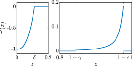
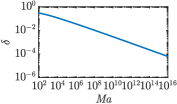
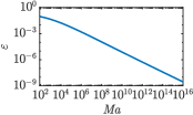
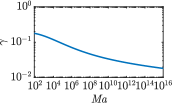
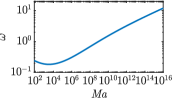
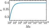
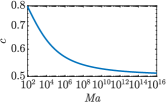
Figure 1: (a) Bounds on Nu obtained with (22) for optimised $\delta$, $\varepsilon$, $\gamma$, $s$, $\omega$, $c$ (           ), and with (27) for $\varepsilon=\mbox{\it Ma}^{-1/2}$, $s=\frac{2}{5}$, $c=\frac{1}{2}$ and either $\gamma=\frac{1}{2}$ ( ) or $\gamma=(\ln\mbox{\it Ma})^{-1}$ (     ). Also plotted are the analytical bound $\mbox{\it Nu}\leq 0.838\mbox{\it Ma}^{2/7}$ by Hagstrom & Doering (2010) (     ), the numerical bound by Fantuzzi et al. (2018) ( ), and DNS data by Boeck & Thess (2001) (x). (b–c) Optimised boundary layers of $\tau^{\prime}$ for $\mbox{\it Ma}=10^{4}$. (d–i) Values of $\delta$, $\varepsilon$, $\gamma$, $\omega$, $s$ and $c$ that optimise (22) subject to (20a,b), $\delta<\frac{1}{2}$, $\varepsilon<\gamma\leq\frac{1}{2}$ and $0<c<1$, as a function of Ma.

First, for simplicity we strengthen (20b) by estimating $\varphi(\gamma,\delta)\geq\varphi(\gamma,\frac{1}{2})$, cf. (21). Then, it follows from (22) that $\delta$ should be taken as large as the resulting inequality allows. Upon insisting that

$$\omega\varepsilon^{2}=\frac{4(1-c)^{2}}{\mbox{\it Ma}}$$ (25)

at all Ma, which is the case for the optimal parameters obtained numerically, we find

$$\delta=\left[\frac{441}{\mbox{\it Ma}^{2}}c^{2}(1-c)^{2}(2+7s)^{2}(1-\gamma)\ln\left(\frac{\gamma}{\varepsilon}\right)\varphi\left(\gamma,\tfrac{1}{2}\right)\right]^{\frac{1}{7}}.$$ (26)

Substituting this expression back into (22) and using (25) to eliminate $\omega$ yields

$$\mbox{\it Nu}^{-1}\geq A(\gamma,\varepsilon,c,s)-B(\gamma,\varepsilon,c),$$ (27)

where

$$A(\gamma,\varepsilon,c,s):=\frac{2}{2+s}\left[\frac{441}{\mbox{\it Ma}^{2}}c^{2}(1-c)^{2}(2+7s)^{2}(1-\gamma)\ln\left(\frac{\gamma}{\varepsilon}\right)\varphi\left(\gamma,\tfrac{1}{2}\right)\right]^{\frac{1}{7}},$$

$$B(\gamma,\varepsilon,c):=\frac{16(1-c)^{4}}{3\mbox{\it Ma}^{2}\varepsilon^{3}}\left(1-\frac{\varepsilon}{\gamma}\right)\left(\frac{3\mbox{\it Ma}\,\varepsilon^{2}}{2(1-c)^{2}}+1+\frac{\varepsilon}{\gamma}+\frac{\varepsilon^{2}}{\gamma^{2}}\right).$$

To proceed, we make two suboptimal but simple choices. First, to simplify the dependence of $B(\gamma,\varepsilon,c)$ on Ma we set $\varepsilon=\mbox{\it Ma}^{-\frac{1}{2}}.$ This gives $\omega=4(1-c)^{2}$ by (25). Second, motivated by our computational results we assume that $\gamma/\varepsilon=\gamma\mbox{\it Ma}^{\frac{1}{2}}\to\infty$ as Ma tends to infinity. Then, $B(\gamma,\mbox{\it Ma}^{-\frac{1}{2}},c)$ decays to zero faster than $A(\gamma,\mbox{\it Ma}^{-\frac{1}{2}},c,s)$ as Ma is raised and we conclude from (27) that, asymptotically, $\mbox{\it Nu}\leq 1/A(\gamma,\mbox{\it Ma}^{-\frac{1}{2}},c,s)$. Minimising this asymptotic bound over $s$ and $c$ simply requires maximising $A(\gamma,\mbox{\it Ma}^{-\frac{1}{2}},c,s)$. This is straightforward and yields $s=\frac{2}{5}$ and $c=\frac{1}{2}$, the same values approached by the optimal parameters in figure 1(h,i). With these values, (26) reduces to the value in (24b) and the asymptotic bound on Nu becomes

$$\mbox{\it Nu}\leq\frac{6}{5}\left[\frac{126^{2}}{25}\frac{1}{\mbox{\it Ma}^{2}}(1-\gamma)\ln\left(\gamma\mbox{\it Ma}^{\frac{1}{2}}\right)\varphi\left(\gamma,\tfrac{1}{2}\right)\right]^{-\frac{1}{7}}\quad{\rm as}\quad\mbox{\it Ma}\to\infty.$$ (28)

Minimising this expression over $\gamma$ is not possible analytically, but is also not necessary in order to prove (23). For instance, simply setting $\gamma=\frac{1}{2}$ gives

$$\mbox{\it Nu}\leq\frac{6}{5}\left[\frac{126^{2}}{100}\varphi\left(\tfrac{1}{2},\tfrac{1}{2}\right)\right]^{-\frac{1}{7}}\times\frac{\mbox{\it Ma}^{\frac{2}{7}}}{(\ln\mbox{\it Ma})^{\frac{1}{7}}}\quad{\rm as}\quad\mbox{\it Ma}\to\infty.$$

Moreover, in light of (21) the prefactor can be improved by letting $\gamma\to 0$ as $\mbox{\it Ma}\to\infty$, which asymptotically optimises the term $(1-\gamma)\varphi(\gamma,\tfrac{1}{2})$ in (28). The decay of $\gamma$ must be sufficiently slow to ensure that $\gamma\mbox{\it Ma}^{\frac{1}{2}}\to\infty$, as assumed above. With $\gamma=(\ln\mbox{\it Ma})^{-1}$, for instance,

$$\mbox{\it Nu}\leq\frac{6}{5}\left[\frac{126^{2}}{50}\varphi\left(0,\tfrac{1}{2}\right)\right]^{-\frac{1}{7}}\times\frac{\mbox{\it Ma}^{\frac{2}{7}}}{(\ln\mbox{\it Ma})^{\frac{1}{7}}}\quad{\rm as}\quad\mbox{\it Ma}\to\infty.$$

The exact bounds on Nu obtained from (27) at finite Ma for ${\varepsilon=\mbox{\it Ma}^{-\frac{1}{2}}}$, $c=\frac{1}{2}$, $s=\frac{2}{5}$ and either $\gamma=\frac{1}{2}$ or $\gamma=(\ln\mbox{\it Ma})^{-1}$ are plotted in figure 1(a).

5 Conclusion

In this paper we have derived a new rigorous bound for the Nusselt number in Pearson’s model of Bénard–Marangoni convection at infinite Prandtl number. Specifically, we have proven that $\mbox{\it Nu}\lesssim\mbox{\it Ma}^{2/7}(\ln\mbox{\it Ma})^{-1/7}$ at asymptotically high Ma, thereby refining a pure power-law bound with exponent 2/7 by Hagstrom & Doering (2010). The quantitative improvement on this previous result is not large for realistic values of the Marangoni number, but our logarithmic correction is significant for two reasons.

First, its proof relies on a subtle balance between the width of the bottom boundary layer of our background temperature field, which drives the asymptotic scaling of Nu, and the stabilising effect – with respect to the marginal stability constraint (9) – of a thin layer near the fluid’s surface where the temperature increases. Qualitatively similar layers characterise the mean vertical temperature profiles observed in DNS by Boeck & Thess (2001, Figure 2) and their coupling underpins the phenomonological scaling theory proposed by those authors. It is therefore tempting to conjecture that the heat transport in physically realised flows indeed depends on a subtle interplay between the thermal boundary layers. In order to test this hypothesis thoroughly, it would be desirable to perform numerical simulations at higher Marangoni numbers than those considered by Boeck & Thess (2001). Further DNS would also enable one to check if our rigorous bound is sharp and if the assumptions in Boeck & Thess’ scaling argument (most notably, the stability of simple steady convection rolls) should be revised.

Second, our result is the first upper bound proven with the background method that has a logarithmic correction with negative exponent. This is reminiscent of scaling laws obtained for wall-bounded flows through “mixing length” turbulent theories (see, e.g., chapter 3 in Doering & Gibbon, 1995). While we are not aware of any such theories being applied to Bénard–Marangoni convection, they have historically motivated the development of rigorous upper-bounding theory in general, and the background method in particular (Doering & Constantin, 1992). In the future, it would be interesting to see if bounds with logarithmic corrections with negative exponent are provable for other flows, starting with extensions of the basic model considered in this work to more general types of thermal boundary conditions (e.g., Pearson, 1958; Fantuzzi & Wynn, 2017).

Declaration of Interests. The authors report no conflict of interest.

Appendix A Estimates on $f_{k}(z)$

For the lower bound on $f_{k}(z)$ in (7), observe that the functions $h(kz)$ and $h[k(1-z)]$ are, respectively, increasing and decreasing on $[\beta,1]$ for any fixed $k>0$ . This means that the function $|f_{k}(z)|(1-z)^{-1}$ increases on $[\beta,1]$, which yields the lower bound.

For the upper bound in (7), instead, rewrite (5) as

$$\left|f_{k}(z)\right|=\frac{k(1-z)}{2}e^{-k(1-z)}g_{k}(z)$$ (29)

with

$$g_{k}(z):=\frac{h(k)h(kz)-h(k(1-z))}{h(2k)-1}\,kze^{k(1-z)}.$$

Differentiation gives

$$g_{k}^{\prime}(z)=\frac{e^{2k(1-z)}\ell_{k}(z)}{2(h(2k)-1)(1-z)^{2}},$$

with $\ell_{k}(z):=e^{-2k}\left(e^{2kz}\!\!\!-\!(1\!-\!z)^{2}\right)+z^{2}(1\!-\!2k)+2z(k\!-\!1).$ Now, $\ell_{k}(0)=0=\ell_{k}(1)$ and $\ell_{k}^{\prime}(0)>0$. Further, $\ell_{k}^{\prime}$ is the sum of a convex and a linear function, meaning that $\ell_{k}$ has at most two stationary points. Since $\ell_{k}^{\prime}(1)=0$, there is at most one stationary point in $0<z<1$. Thus, both $\ell_{k}(z)\geq 0$ and $g_{k}^{\prime}(z)\geq 0$ for $z\in[0,1]$. From this we conclude that

$$g_{k}(z)\leq g_{k}(1)=k\left[h(k)^{2}-1\right]\left[h(2k)-1\right]^{-1}\leq 1,$$

which, by (29), proves the upper bound in (7).

Finally, to show (6), use the definition of $h$ and the inequalities $1\leq x\coth x\leq 1+\frac{x^{2}}{3},$ which are valid for $x\geq 0$, to obtain

$$(z-1)\frac{h[k(1-z)]}{h(k)h(kz)}=kz\left[\coth(k)-\coth(kz)\right]\leq z\left(1+\tfrac{1}{3}k^{2}\right)-1.$$

Combining this estimate with equation (5) and the identity $\left|f_{k}\right|=-f_{k}$ gives

$$\left|f_{k}(z)\right|\leq\frac{1}{2}k^{2}z\frac{h(k)h(kz)}{h(2k)-1}\left[1-z+z\left(1+\tfrac{1}{3}k^{2}\right)-1\right]=\frac{1}{6}k^{4}\frac{h(k)h(kz)}{h(2k)-1}z^{2}.$$

Since $h$ is increasing, so $h(kz)\leq h(k\beta)$ for all $z\in[0,\beta]$, the upper bound (6) follows.

References

Bénard (1901)Bénard, H. 1901 Les tourbillons cellulaires dans une
nappe liquide—méthodes optiques d’observation et d’enregistrement.
J. Phys. Theor. Appl.10 (1), 254–266.
Boeck (2005)Boeck, T. 2005 Bénard–Marangoni convection at
large Marangoni numbers: Results of numerical simulations. Adv. Space
Res.36 (1), 4–10.
Boeck & Thess (1998)Boeck, T. & Thess, A. 1998 Turbulent
Bénard–Marangoni Convection: Results of Two-Dimensional Simulations.
Phys. Rev. Lett.80 (6), 1216–1219.
Boeck & Thess (2001)Boeck, T. & Thess, A. 2001 Power-law scaling in
Bénard–Marangoni convection at large Prandtl numbers. Phys.
Rev. E64 (2), 027303.
DebRoy & David (1995)DebRoy, T. & David, S. A. 1995 Physical processes
in fusion welding. Rev. Modern Phys.67 (1), 85–112.
Doering & Constantin (1992)Doering, C. R. & Constantin, P. 1992 Energy
dissipation in shear driven turbulence. Phys. Rev. Lett.69 (11), 1648–1651.
Doering & Gibbon (1995)Doering, C. R. & Gibbon, J. D. 1995 Applied
analysis of the Navier–Stokes equations. Cambridge Texts in Applied
Mathematics 12. Cambridge University Press.
Doering et al. (2006)Doering, C. R., Otto, F. & Reznikoff, M. G. 2006
Bounds on vertical heat transport for infinite Prandtl number
Rayleigh–Bénard convection. J. Fluid Mech.560,
229–241.
Fantuzzi et al. (2018)Fantuzzi, G., Pershin, A. & Wynn, A. 2018
Bounds on heat transfer for Bénard–Marangoni convection at infinite
Prandtl number. J. Fluid Mech.837, 562–596.
Fantuzzi & Wynn (2017)Fantuzzi, G. & Wynn, A. 2017 Exact energy stability
of Bénard–Marangoni convection at infinite Prandtl number. J.
Fluid Mech.822, R1.
Hagstrom & Doering (2010)Hagstrom, G. I. & Doering, C. R. 2010 Bounds on
heat transport in Bénard–Marangoni convection. Phys. Rev. E81 (4), 047301.
Lappa (2010)Lappa, M. 2010 Thermal Convection: Patterns, Evolution
and Stability. John Wiley & Sons Ltd.
Malkus (1954)Malkus, W. V. R. 1954 The heat transport and spectrum of
thermal turbulence. Proc. Roy. Soc. London Ser. A225 (1161),
196–212.
Pearson (1958)Pearson, J. R. A. 1958 On convection cells induced by
surface tension. J. Fluid Mech.4 (5), 489–500.
Pumir & Blumenfeld (1996)Pumir, A. & Blumenfeld, L. 1996 Heat transport in a
liquid layer locally heated on its free surface. Phys. Rev. E54 (5), R4528–R4531.
Whitehead & Doering (2011)Whitehead, J. P. & Doering, C. R. 2011 Internal
heating driven convection at infinite Prandtl number. J. Math. Phys.52 (9), 093101.
Whitehead & Wittenberg (2014)Whitehead, J. P. & Wittenberg, R. W. 2014 A
rigorous bound on the vertical transport of heat in Rayleigh-Bénard
convection at infinite Prandtl number with mixed thermal boundary
conditions. J. Math. Phys.55 (9), 093104.