Anomaly Detection with Inexact Labels

Abstract

We propose a supervised anomaly detection method for data with inexact anomaly labels, where each label, which is assigned to a set of instances, indicates that at least one instance in the set is anomalous. Although many anomaly detection methods have been proposed, they cannot handle inexact anomaly labels. To measure the performance with inexact anomaly labels, we define the inexact AUC, which is our extension of the area under the ROC curve (AUC) for inexact labels. The proposed method trains an anomaly score function so that the smooth approximation of the inexact AUC increases while anomaly scores for non-anomalous instances become low. We model the anomaly score function by a neural network-based unsupervised anomaly detection method, e.g., autoencoders. The proposed method performs well even when only a small number of inexact labels are available by incorporating an unsupervised anomaly detection mechanism with inexact AUC maximization. Using various datasets, we experimentally demonstrate that our proposed method improves the anomaly detection performance with inexact anomaly labels, and outperforms existing unsupervised and supervised anomaly detection and multiple instance learning methods.

1 Introduction

Anomaly detection is an important machine learning task, which is a task to find the anomalous instances in a dataset. Anomaly detection has been used in a wide variety of applications (Chandola et al., 2009; Patcha and Park, 2007; Hodge and Austin, 2004), such as network intrusion detection for cyber-security (Dokas et al., 2002; Yamanishi et al., 2004), fraud detection for credit cards (Aleskerov et al., 1997), defect detection in industrial machines (Fujimaki et al., 2005; Idé and Kashima, 2004) and disease outbreak detection (Wong et al., 2003).

Many unsupervised anomaly detection methods have been proposed (Breunig et al., 2000; Schölkopf et al., 2001; Liu et al., 2008; Sakurada and Yairi, 2014). When anomaly labels, which indicate whether each instance is anomalous, are given, the anomaly detection performance can be improved (Singh and Silakari, 2009; Mukkamala et al., 2005; Rapaka et al., 2003; Nadeem et al., 2016; Gao et al., 2006; Das et al., 2016, 2017). However, it is difficult to attach exact anomaly labels in some situations. Consider such example in server system failure detection. System operators often do not know the exact time of failures; they only know that a failure occurred within a certain period of time. In this case, anomaly labels can be attached to instances in a certain period of time, in which non-anomalous instances might be included. Another example is detecting anomalous IoT devices connected to a server. Even when the server displays unusual behavior, we sometimes cannot identify which IoT devices are anomalous. In these situations, only inexact anomaly labels are available.

In this paper, we propose a supervised anomaly detection method for data with inexact anomaly labels. An inexact anomaly label is attached to a set of instances, indicating that at least one instance in the set is anomalous. We call this set an inexact anomaly set. First, we define an extension of the area under the ROC curve (AUC) for performance measurement with inexact labels, which we call an inexact AUC. Then we develop an anomaly detection method that maximizes the inexact AUC. With the proposed method, a function, which outputs an anomaly score given an instance, is modeled by the reconstruction error with autoencoders, which are a successfully used neural network-based unsupervised anomaly detection method (Sakurada and Yairi, 2014; Sabokrou et al., 2016; Chong and Tay, 2017; Zhou and Paffenroth, 2017). Note that the proposed method can use any unsupervised anomaly detection methods with learnable parameters instead of autoencoders, such as variational autoencoders (Kingma and Wellniga, 2014), energy-based models (Zhai et al., 2016), and isolation forests (Liu et al., 2008). The parameters of the anomaly score function are trained so that the anomaly scores for non-anomalous instances become low while the smooth approximation of the inexact AUC becomes high. Since our objective function is differentiable, the anomaly score function can be estimated efficiently using stochastic gradient-based optimization methods.

The proposed method performs well even when only a few inexact labels are given since it incorporates an unsupervised anomaly detection mechanism, which works without label information. In addition, the proposed method is robust to class imbalance since our proposed inexact AUC maximization is related to AUC maximization, which achieved high performance on imbalanced data classification tasks (Cortes and Mohri, 2004). Class imbalance robustness is important for anomaly detection since anomalous instances occur more rarely than non-anomalous instances.

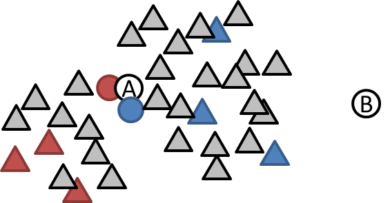
Figure 1: Example of anomalous (circle) and non-anomalous (triangle) instances, and inexact anomaly sets (red or blue) in an instance space. Instances with identical color (red or blue) are contained in the same inexact anomaly set. White circles are test anomalous instances.

Figure 1 shows an example of anomalous and non-anomalous instances, and inexact anomaly sets in a two-dimensional instance space. For unsupervised methods, it is difficult to detect test anomalous instance ‘A’ since some instances are located around it. Unsupervised methods consider that an instance is anomalous when there are few instances around it. Since supervised methods can use label information, they can correctly detect test anomalous instance ‘A’. However, they might not detect test anomalous instance ‘B’ since there are no labeled instances near it. In addition, with supervised methods that consider all the instances in inexact anomaly sets are anomaly, non-anomalous instances around training instances in the inexact anomaly sets (colored triangles in Figure 1) would be misclassified as anomaly. On the other hand, the proposed method detects ‘A’ using label information and ‘B’ by incorporating an unsupervised anomaly detection mechanism. Also, it would not detect non-anomalous instances as anomaly since it can handle inexact information.

The remainder of the paper is organized as follows. In Section 2, we briefly review related work. In Section 3, we introduce AUC, which is the basis of the inexact AUC. In Section 4, we present the inexact AUC, define our task, and propose our method for supervised anomaly detection using inexact labels. In Section 5, we experimentally demonstrate the effectiveness of our proposed method using various datasets by comparing with existing anomaly detection and multiple instance learning methods. Finally, we present concluding remarks and discuss future work in Section 6.

2 Related work

Inexact labels in classification tasks have been considered in multiple instance learning methods (Dietterich et al., 1997; Maron and Lozano-Pérez, 1998; Babenko et al., 2009; Wu et al., 2015; Cinbis et al., 2017), where labeled sets are given for training. For a binary classification task, a set is labeled negative if all the instances in it are negative, and it is labeled positive if it contains at least one positive instance. An advantage of the proposed method over existing multiple instance learning methods is that the proposed method works well with a small number of inexact anomaly labels using inexact AUC maximization and incorporating an unsupervised anomaly detection mechanism, where we exploit the characteristics of anomaly detection tasks. Existing multiple instance learning methods are not robust to class imbalance (Herrera et al., 2016; Carbonneau et al., 2018).

Anomaly detection is also called outlier detection (Hodge and Austin, 2004) or novelty detection (Markou and Singh, 2003). Many unsupervised methods have been proposed, such as the local outlier factor (Breunig et al., 2000), one-class support vector machines (Schölkopf et al., 2001), isolation forests (Liu et al., 2008), and density estimation based methods (Shewhart, 1931; Eskin, 2000; Laxhammar et al., 2009). However, these methods cannot use label information. Although supervised anomaly detection methods have been proposed to exploit label information (Nadeem et al., 2016; Gao et al., 2006; Das et al., 2016, 2017; Munawar et al., 2017; Pimentel et al., 2018; Akcay et al., 2018; Iwata and Yamanaka, 2019), they cannot handle inexact anomaly labels. A number of AUC maximization methods have been proposed (Cortes and Mohri, 2004; Brefeld and Scheffer, 2005; Ying et al., 2016; Fujino and Ueda, 2016; Narasimhan and Agarwal, 2017; Sakai et al., 2018) for training on class imbalanced data. However, these methods do not consider inexact labels.

3 Preliminaries: AUC

Let $\mathcal{X}$ be an instance space, and let $p_{\mathrm{A}}$ and $p_{\mathrm{N}}$ be probability distributions over anomalous and non-anomalous instances in $\mathcal{X}$. Suppose that $a:\mathcal{X}\to\mathbb{R}$ is an anomaly score function, and anomaly detection is carried out based on its sign:

$$\mathrm{sign}(a(\mathbf{x})-h),$$ (1)

where $\mathbf{x}$ is an instance and $h$ is a threshold. The true positive rate (TPR) of anomaly score function $a(\mathbf{x})$ is the rate that it correctly classifies a random anomaly from $p_{\mathrm{A}}$ as anomalous,

$$\mathrm{TPR}(h)=\mathbb{E}_{\mathbf{x}^{\mathrm{A}}\sim p_{\mathrm{A}}}[I(a(\mathbf{x}^{\mathrm{A}})>h)],$$ (2)

where $\mathbb{E}$ is the expectation and $I(\cdot)$ is the indicator function; $I(A)=1$ if $A$ is true, and $I(A)=0$ otherwise. The false positive rate (FPR) is the rate that it misclassifies a random non-anomalous instance from $p_{\mathrm{N}}$ as anomalous,

$$\mathrm{FPR}(h)=\mathbb{E}_{\mathbf{x}^{\mathrm{N}}\sim p_{\mathrm{N}}}[I(a(\mathbf{x}^{\mathrm{N}})>h)].$$ (3)

The ROC curve is the plot of $\mathrm{TPR}(h)$ as a function of $\mathrm{FPR}(h)$ with different threshold $h$. The area under this curve (AUC) (Hanley and McNeil, 1982) is computed as follows (Dodd and Pepe, 2003):

$$\mathrm{AUC}=\int_{0}^{1}\mathrm{TPR}(\mathrm{FPR}^{-1}(s))ds=\mathbb{E}_{\mathbf{x}^{\mathrm{A}}\sim p_{\mathrm{A}},\mathbf{x}^{\mathrm{N}}\sim p_{\mathrm{N}}}[I(a(\mathbf{x}^{\mathrm{A}})>a(\mathbf{x}^{\mathrm{N}}))],$$ (4)

where $\mathrm{FPR}^{-1}(s)=\inf\{h\in\mathbb{R}|\mathrm{FPR}(h)\leq s\}$. AUC is the rate where a randomly sampled anomalous instance has a higher anomaly score than a randomly sampled non-anomalous instance.

Given sets of anomalous instances $\mathcal{A}=\{\mathbf{x}^{\mathrm{A}}_{i}\}_{i=1}^{|\mathcal{A}|}$ drawn from $p_{\mathrm{A}}$ and non-anomalous instances $\mathcal{N}=\{\mathbf{x}^{\mathrm{N}}_{j}\}_{j=1}^{|\mathcal{N}|}$ drawn from $p_{\mathrm{N}}$, an empirical AUC is calculated by

$$\widehat{\mathrm{AUC}}=\frac{1}{|\mathcal{A}||\mathcal{N}|}\sum_{\mathbf{x}_{i}^{\mathrm{A}}\in\mathcal{A}}\sum_{\mathbf{x}_{j}^{\mathrm{N}}\in\mathcal{N}}I(a(\mathbf{x}_{i}^{\mathrm{A}})>a(\mathbf{x}_{j}^{\mathrm{N}})),$$ (5)

where $|\mathcal{A}|$ represents the size of set $\mathcal{A}$.

4 Proposed method

4.1 Inexact AUC

Let $\mathcal{B}=\{\mathbf{x}^{\mathrm{B}}_{i}\}_{i=1}^{|\mathcal{B}|}$ be a set of instances drawn from probability distribution $p_{\mathrm{S}}$, where at least one instance is drawn from anomalous distribution $p_{\mathrm{A}}$, and the other instances are drawn from non-anomalous distribution $p_{\mathrm{N}}$. We define inexact true positive rate (inexact TPR) as the rate where anomaly score function $a(\mathbf{x})$ classifies at least one instance in a random instance set from $p_{\mathrm{S}}$ as anomalous:

$$\mathrm{iTPR}(h)=\mathbb{E}_{\mathcal{B}\sim p_{\mathrm{S}}}\left[I\left(\bigvee_{\mathbf{x}_{i}^{\mathrm{B}}\in\mathcal{B}}\left[a(\mathbf{x}_{i}^{\mathrm{B}})>h)\right]\right)\right]=\mathbb{E}_{\mathcal{B}\sim p_{\mathrm{S}}}\left[I(\max_{x_{i}^{\mathrm{B}}\in\mathcal{B}}a(\mathbf{x}_{i}^{\mathrm{B}})>h)\right].$$ (6)

We then define the inexact AUC by the area under the curve of $\mathrm{iTPR}(h)$ as a function of $\mathrm{FPR}(h)$ with different threshold $h$ in a similar way with the AUC (4) as follows:

$$\mathrm{iAUC}=\int_{0}^{1}\mathrm{iTPR}(\mathrm{FPR}^{-1}(s))ds=\mathbb{E}_{\mathcal{B}\sim p_{\mathrm{S}},\mathbf{x}^{\mathrm{N}}\sim p_{\mathrm{N}}}[I(\max_{\mathbf{x}_{i}^{\mathrm{B}}\in\mathcal{B}}a(\mathbf{x}_{i}^{\mathrm{B}})>a(\mathbf{x}^{\mathrm{N}}))].$$ (7)

Inexact AUC is the rate where at least one instance in a randomly sampled inexact anomaly set has a higher anomaly score than a randomly sampled non-anomalous instance. When the label information is exact, i.e., every inexact anomaly set $\mathcal{B}$ contains only a single anomalous instance, the inexact AUC (7) is equivalent to AUC (4). Therefore, the inexact AUC is a natural extension of the AUC for inexact labels.

Given a set of inexact anomaly sets $\mathcal{S}=\{\mathcal{B}_{k}\}_{k=1}^{|\mathcal{S}|}$, where $\mathcal{B}_{k}=\{\mathbf{x}^{\mathrm{B}}_{ki}\}_{i=1}^{|\mathcal{B}_{k}|}$, drawn from $p_{\mathrm{S}}$, and a set of non-anomalous instances $\mathcal{N}=\{\mathbf{x}^{\mathrm{N}}_{j}\}_{j=1}^{|\mathcal{N}|}$ drawn from $p_{\mathrm{N}}$, we calculate an empirical inexact AUC as follows:

$$\widehat{\mathrm{iAUC}}=\frac{1}{|\mathcal{S}||\mathcal{N}|}\sum_{\mathcal{B}_{k}\in\mathcal{S}}\sum_{\mathbf{x}_{j}^{\mathrm{N}}\in\mathcal{N}}I[\max_{\mathbf{x}^{\mathrm{B}}_{ki}\in\mathcal{B}_{k}}a(\mathbf{x}^{\mathrm{B}}_{ki})>a(\mathbf{x}_{j}^{\mathrm{N}})].$$ (8)

The maximum operator has been widely used for multiple instance learning methods (Maron and Lozano-Pérez, 1998; Andrews et al., 2003; Pinheiro and Collobert, 2015; Zhu et al., 2017; Feng and Zhou, 2017; Ilse et al., 2018). The proposed inexact AUC can evaluate score functions properly even with class imbalanced data by incorporating the maximum operator into the AUC framework.

4.2 Task

Suppose that we are given a set of inexact anomaly sets $\mathcal{S}$ and a set of non-anomalous instances $\mathcal{N}$ for training. Our task is to estimate anomaly scores of test instances, which are not included in the training data, so that the anomaly score is high when the test instance is anomalous, and low when it is non-anomalous.

Table 1: Our notation

Symbol	Description
$\mathcal{S}$	set of inexact anomaly sets, $\{\mathcal{B}_{k}\}_{k=1}^{|\mathcal{S}|}$
$\mathcal{B}_{k}$	$k$th inexact anomaly set, where at least one instance is anomaly, $\{\mathbf{x}^{\mathrm{B}}_{ki}\}_{i=1}^{|\mathcal{B}_{k}|}$
$\mathcal{A}$	set of anomalous instances, $\{\mathbf{x}^{\mathrm{A}}_{i}\}_{i=1}^{|\mathcal{A}|}$
$\mathcal{N}$	set of non-anomalous instances, $\{\mathbf{x}^{\mathrm{N}}_{j}\}_{j=1}^{|\mathcal{N}|}$
$a(\mathbf{x})$	anomaly score of instance $\mathbf{x}$

4.3 Anomaly scores

For the anomaly score function, we use the following reconstruction error with deep autoencoders:

$$a(\mathbf{x};\bm{\theta})=\parallel\mathbf{x}-g(f(\mathbf{x};\bm{\theta}_{\mathrm{f}});\bm{\theta}_{\mathrm{g}})\parallel^{2},$$ (9)

where $f(\cdot;\bm{\theta}_{\mathrm{f}})$ is an encoder modeled by a neural network with parameters $\bm{\theta}_{\mathrm{f}}$, $g(\cdot;\bm{\theta}_{\mathrm{g}})$ is a decoder modeled by a neural network with parameters $\bm{\theta}_{\mathrm{g}}$, and $\bm{\theta}=\{\bm{\theta}_{\mathrm{f}},\bm{\theta}_{\mathrm{g}}\}$ is the parameters of the anomaly score function. The reconstruction error of an instance is likely to be low when instances similar to it often appear in the training data, and the reconstruction error is likely to be high when no similar instances are contained in the training data. With the proposed method, we can use other anomaly score functions that are differentiable with respect to parameters, such as Gaussian mixtures (Eskin, 2000; An and Cho, 2015; Suh et al., 2016; Xu et al., 2018), variational autoencoders (Kingma and Wellniga, 2014), energy-based models (Zhai et al., 2016), and isolation forests (Liu et al., 2008).

4.4 Objective function

With the proposed method, parameters $\bm{\theta}$ are trained by minimizing the anomaly scores for non-anomalous instances while maximizing the empirical inexact AUC (8). To make the empirical inexact AUC differentiable with respect to the parameters, we use sigmoid function $\sigma(A-B)=\frac{1}{1+\exp(-(A-B))}$ instead of step function $I(A>B)$, which is often used for a smooth approximation of the step function. Then the objective function to be minimized is given:

$$E=\frac{1}{|\mathcal{N}|}\sum_{\mathbf{x}_{j}^{\mathrm{N}}\in\mathcal{N}}a(\mathbf{x}_{j}^{\mathrm{N}})-\lambda\frac{1}{|\mathcal{S}||\mathcal{N}|}\sum_{\mathcal{B}_{k}\in\mathcal{S}}\sum_{\mathbf{x}_{j}^{\mathrm{N}}\in\mathcal{N}}\sigma\left(\max_{\mathbf{x}^{\mathrm{B}}_{ki}\in\mathcal{B}_{k}}a(\mathbf{x}^{\mathrm{B}}_{ki})-a(\mathbf{x}_{j}^{\mathrm{N}})\right),$$ (10)

where $\lambda\geq 0$ is a hyperparameter that can be tuned using the inexact AUC on the validation data. When there are no inexact anomaly sets or $\lambda=0$, the second term becomes zero, and the first term on the non-anomalous instances remains with the objective function, which is the same objective function with a standard autoencoder. By the unsupervised anomaly detection mechanism of the first term in (10), the proposed method can detect anomalous instances even when there are few inexact anomaly sets. The computational complexity of calculating the objective function (10) is $O(|\mathcal{S}||\mathcal{B}|+|\mathcal{S}||\mathcal{N}|)$, where $|\mathcal{B}|$ is the average number of instances in an inexact anomaly set, the first term is for finding the maximum of anomaly scores in every inexact anomaly set, and the second term is for calculating the difference of scores between inexact anomalous instances and non-anomalous instances in the second term in (10).

5 Experiments

5.1 Data

We evaluated our proposed supervised anomaly detection method with a synthetic dataset and nine datasets used for unsupervised anomaly detection (Campos et al., 2016) .

The synthetic dataset was generated from a two-dimensional Gaussian mixture model shown in Figure 2(a,b). The non-anomalous instances were generated from two unit-variance Gaussian distributions with mean at (-2,0) and (2,0), as shown by blue triangles in Figure 2(a). The anomalous instances were generated from a Gaussian distribution with mean (0,-1.5) with a small variance and a Gaussian distribution with mean (0,3) with a wide variance as shown by red circles in Figure 2(a). The latter anomalous Gaussian was only used for test data, and it was not used for training and validation data as shown in Figure 2(b). We generated 500 instances from the non-anomalous Gaussians, and 200 instances from the anomalous Gaussians.

Table 2 shows the following values of the nine anomaly detection datasets: the number of anomalous instances $|\mathcal{A}|$, the number of non-anomalous instances $|\mathcal{N}|$, anomaly ratio $\frac{|\mathcal{A}|}{|\mathcal{N}|}$, and the number of attributes $D$. Each attribute was linearly normalized to range $[0,1]$, and duplicate instances were removed. The original datasets contained only exact anomaly labels (Campos et al., 2016). We constructed inexact anomaly sets by randomly sampling non-anomalous instances and an anomalous instance for each set.

We used 70% of the non-anomalous instances and ten inexact anomaly sets for training, 15% of the non-anomalous instances and five inexact anomaly sets for validation, and the remaining instances for testing. The number of instances in an inexact anomaly set was five with training and validation data, and one with test data; the test data contained only exact anomaly labels. For each inexact anomaly set, we included an anomalous instance, and the other instances were non-anomalous. For the evaluation measurement, we used AUC on test data. For each dataset, we randomly generated ten sets of training, validation and test data, and calculated the average AUC over the ten sets.

Table 2: Statistics of datasets used in our experiments. $|\mathcal{A}|$ is the number of anomalous instances, $|\mathcal{N}|$ is the number of non-anomalous instances, and $D$ is the number of attributes.

Data	$|\mathcal{A}|$	$|\mathcal{N}|$	$\frac{|\mathcal{A}|}{|\mathcal{N}|}$	$D$
Annthyroid	350	6666	0.053	21
Cardiotocography	413	1655	0.250	21
InternetAds	177	1598	0.111	1555
KDDCup99	246	60593	0.004	79
PageBlocks	258	4913	0.053	10
Pima	125	500	0.250	8
SpamBase	697	2788	0.250	57
Waveform	100	3343	0.030	21
Wilt	93	4578	0.020	5

5.2 Comparing methods

We compared our proposed method with the following 11 methods: LOF, OSVM, IF, AE, KNN, SVM, RF, NN, MIL, SIF and SAE. LOF, OSVM, IF and AE are unsupervised anomaly detection methods, where attribute $\mathbf{x}$ is used for calculating the anomaly score, but the label information is not used for training. KNN, SVM, RF, NN, MIL, SIF, SAE and our proposed method are supervised anomaly detection methods, where both the attribute $\mathbf{x}$ and the label information are used. Since KNN, SVM, RF, NN, SIF and SAE cannot handle inexact labels, they assume that all the instances in the inexact anomaly sets are anomalous. For hyperparameter tuning, we used the AUC scores on the validation data with LOF, OSVM, IF, AE, KNN, SVM, RF, NN, SIF and SAE, and inexact AUC with MIL and our proposed method. We used the scikit-learn implementation (Pedregosa et al., 2011) with LOF, OSVM, IF, KNN, SVM, RF and NN.

LOF, which is the local outlier factor method (Breunig et al., 2000), unsupervisedly detects anomalies based on the degree of isolation from the surrounding neighborhood. The number of neighbors was tuned from $\{1,3,5,15,35\}$ using the validation data.

OSVM is the one-class support vector machine (Schölkopf et al., 2001), which is an extension of the support vector machine (SVM) for unlabeled data. OSVM finds the maximal margin hyperplane, which separates the given non-anomalous data from the origin by embedding them in a high-dimensional space by a kernel function. We used the RBF kernel, its kernel hyperparameter was tuned from $\{10^{-3},10^{-2},10^{-1},1\}$, and hyperparameter $\nu$ was tuned from $\{10^{-3},5\times 10^{-3},10^{-2},5\times 10^{-2},10^{-1},0.5,1\}$.

IF is the isolation forest method (Liu et al., 2008), which is a tree-based unsupervised anomaly detection scheme. IF isolates anomalies by randomly selecting an attribute and randomly selecting a split value between the maximum and minimum values of the selected attribute. The number of base estimators was chosen from $\{1,5,10,20,30\}$.

AE calculates the anomaly score by the reconstruction error with the autoencoder, which is also used with the proposed method. We used the same parameter setting with the proposed method for AE, which is described in the next subsection. Although the model of the proposed method with $\lambda=0$ is the same with that of AE, early stopping criteria were different, where the proposed method used the inexact AUC, and AE used the AUC.

KNN is the $k$-nearest neighbor method, which classifies instances based on the votes of neighbors. The number of neighbors was selected from $\{1,3,5,15\}$.

SVM is a support vector machine (Schölkopf et al., 2002), which is a kernel-based binary classification method. We used the RBF kernel, and the kernel hyperparameter was tuned from $\{10^{-3},10^{-2},10^{-1},1\}$.

RF is the random forest method (Breiman, 2001), which is a meta estimator that fits a number of decision tree classifiers. The number of trees was chosen from $\{5,10,20,30\}$.

NN is a feed-forward neural network classifier. We used three layers with rectified linear unit (ReLU) activation, where the number of hidden units was selected from $\{5,10,50,100\}$.

MIL is a multiple instance learning method based on an autoencoder, which is trained by maximizing the inexact AUC. We used the same parameter setting with the proposed method for the autoencoder. The proposed method with $\lambda=\infty$ corresponds to MIL.

SIF is a supervised anomaly detection method based on the isolation forest (Das et al., 2017), where the weights of the isolation forest are adjusted by maximizing the AUC.

SAE is a supervised anomaly detection method based on an autoencoder, where the neural networks are learned by minimizing the reconstruction error while maximizing the AUC. We used the same parameter setting with the proposed method for the autoencoder.

5.3 Settings of the proposed method

We used three-layer feed-forward neural networks for the encoder and decoder, where the hidden unit size was 128, and the output layer of the encoder and the input layer of the decoder was 16. Hyperparameter $\lambda$ was selected from $\{0,10^{-3},10^{-2},10^{-1},1,10,10^{2},10^{3}\}$ using the inexact AUC on the validation data. The validation data were also used for early stopping, where the maximum number of training epochs was 1000. We optimized the neural network parameters using ADAM (Kingma and Ba, 2015) with learning rate $10^{-3}$, where we randomly sampled eight inexact anomaly sets and 128 non-anomalous instances for each batch. We implemented all the methods based on PyTorch (Paszke et al., 2017).

5.4 Results

Figure 2 shows the estimated anomaly scores by AE (c), SAE (d), MIL (e) and the proposed method (f) on the synthetic dataset. Figure 3 shows the ROC curve and test AUC by the AE (a), SAE (b), MIL (c) and the proposed method (d) on the synthetic dataset. The test AUCs were 0.919 with AE, 0.790 with SAE, 0.905 with MIL, and 0.982 with the proposed method. The AE successfully gave relatively high anomaly scores to the test anomalous instances at the top in Figure 2(c). However, since the AE is an unsupervised method and cannot use label information, some anomalous instances at the bottom center were misclassified as non-anomaly. The SAE is a supervised method, therefore the anomalous instances at the bottom center in Figure 2(d) were identified as anomaly more appropriately than the AE. However, since the SAE cannot handle inexact labels, some test non-anomalous instances, that were located around non-anomalous instances in the training inexact anomaly sets, were falsely classified as anomaly. The MIL correctly gave lower anomaly scores to test non-anomalous instances by handling inexact labels than the SAE in Figure 2(e). However, the MIL failed to correctly give high anomaly scores to unseen anomalous instances at the top. On the other hand, because the proposed method is trained by minimizing the anomaly scores for non-anomalous instances while maximizing the inexact AUC, the proposed method succeeded to detect unseen anomalous instances at the top as well as anomalous instances at the bottom center, and correctly classified test non-anomalous instances as non-anomaly in Figure 2(f).

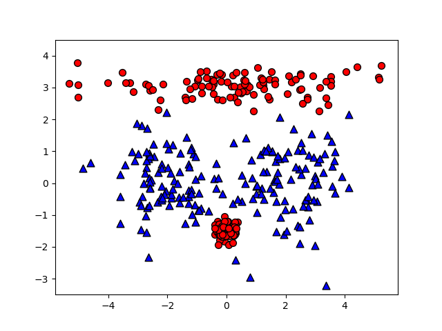
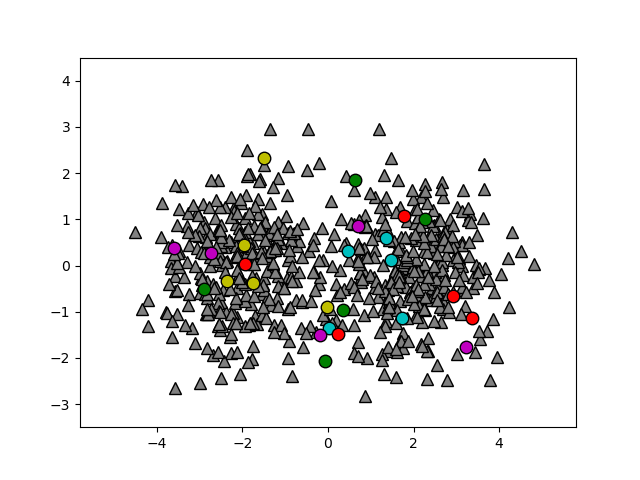
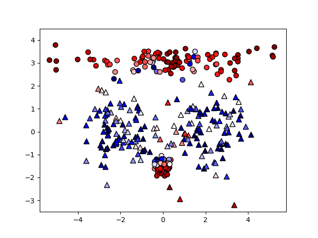
(a) Test data with true labels	(b) Training data	(c) AE
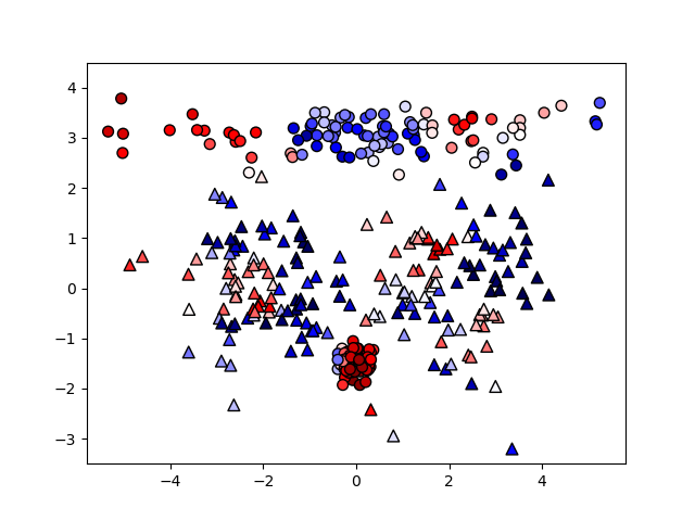
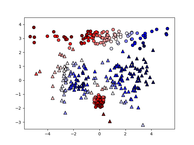
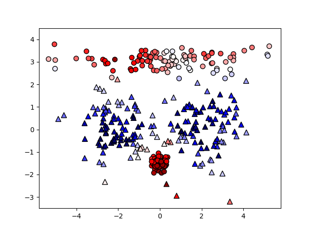
(d) SAE	(e) MIL	(f) Ours

Figure 2: Synthetic dataset and the estimated anomaly scores in the two-dimensional instance space. (a) Test data: anomalous instances are represented by red circles and non-anomalous instances are represented by blue triangles. (b) Training data: instances in the same inexact anomalous set are represented by circles with identical color, and non-anomalous instances are represented by gray triangles. Note that anomalous instances at the top in the test data are not contained in the training data. (c–f) Estimated anomaly scores by the AE (c), SAE (d), MIL (e) and the proposed method (f). The shape indicates the true label (circle: anomalous, triangle: non-anomalous), the color indicates the estimated anomaly score; the darker red indicates the higher anomaly score, and the darker blue indicates lower anomaly score.

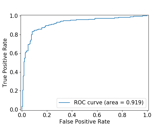
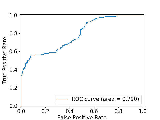
(a) AE	(b) SAE
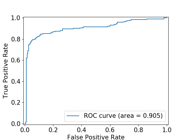
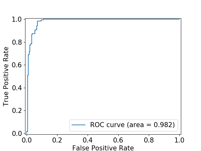
(c) MIL	(d) Ours

Figure 3: ROC curve and AUC on the test synthetic dataset by (a) AE, (b) SAE, (c) MIL, and (d) the proposed method. X-axis is the false positive rate, and y-axis is the true positive rate.

Table 3 shows AUC on the nine anomaly detection datasets with ten inexact anomaly sets and five instances per set. Our proposed method achieved the highest AUC in most cases. Since the number of supervised labels was small, the performance of the supervised methods, KNN, SVM, RF and MIL, was not high. The proposed method outperformed them by incorporating an unsupervised method (AE) in a supervised framework. SIF and SAE also used both unsupervised and supervised anomaly detection frameworks. However, the performance was worse than the proposed method because SIF and SAE cannot handle inexact labels. Although MIL can handle inexact labels, AUC with MIL was low since it does not have an unsupervised training mechanism, i.e., it does not minimize anomaly scores for non-anomalous instances. The average computational time for training the proposed method was 1.0, 0.4, 1.4, 8.1, 0.7, 0.2, 0.5, 0.6 and 0.7 minutes with Annthyroid, Cardiotocography, InternetAds, KDDCup99, PageBlocks, Pima, SpamBase, Waveform and Wilt datasets, respectively, on computers with 2.60GHz CPUs.

Table 3: AUC on nine anomaly detection datasets with ten inexact anomaly sets and five instances per set. Values in bold typeface are not statistically different (at 5% level) from the best performing method in each dataset according to a paired t-test. The Average column shows the average AUC over all datasets, and the value in bold indicates the best average AUC.

	Annthyroid	Cardiotocography	InternetAds	KDDCup99	PageBlocks
LOF	0.652	0.544	0.728	0.576	0.754
OSVM	0.525	0.845	0.814	0.974	0.877
IF	0.768	0.809	0.549	0.973	0.924
AE	0.754	0.768	0.839	0.995	0.915
KNN	0.546	0.639	0.602	0.804	0.672
SVM	0.751	0.725	0.864	0.708	0.599
RF	0.868	0.806	0.622	0.895	0.862
NN	0.622	0.702	0.783	0.975	0.462
MIL	0.590	0.801	0.824	0.714	0.609
SIF	0.829	0.843	0.622	0.992	0.932
SAE	0.836	0.768	0.832	0.924	0.926
Ours	0.867	0.846	0.828	0.992	0.914

	Pima	SpamBase	Waveform	Wilt	Average
LOF	0.601	0.546	0.680	0.709	0.643
OSVM	0.686	0.639	0.622	0.571	0.728
IF	0.714	0.703	0.660	0.617	0.746
AE	0.678	0.757	0.671	0.895	0.808
KNN	0.536	0.617	0.627	0.557	0.622
SVM	0.495	0.573	0.729	0.665	0.679
RF	0.649	0.751	0.711	0.774	0.771
NN	0.396	0.782	0.724	0.619	0.674
MIL	0.670	0.660	0.640	0.474	0.665
SIF	0.706	0.808	0.723	0.703	0.795
SAE	0.662	0.765	0.728	0.863	0.812
Ours	0.713	0.791	0.746	0.895	0.844

Figure 4 shows test AUCs averaged over the nine anomaly detection datasets by changing the number of training inexact anomaly sets (a), and by changing the number of instances per inexact anomaly set (b). The proposed method achieved the best performance in all cases. As the number of training inexact anomaly sets increased, the performance with supervised methods was improved. As the number of instances per inexact anomaly set increased, AUC was decreased since the rate of non-anomalous instances in an inexact anomaly set increased. AUC with unsupervised methods also decreased since they used inexact anomaly sets in the validation data.

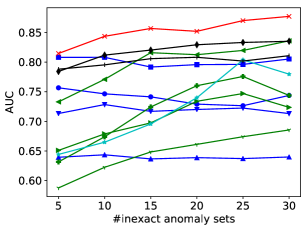
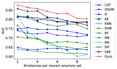
(a) number of inexact anomaly sets	(b) number of instances per inexact anomaly set

Figure 4: AUC averaged over the nine anomaly detection datasets (a) with different numbers of training inexact anomaly sets and five instances per inexact anomaly set, and (b) with different numbers of instances per inexact anomaly set and ten training inexact anomaly sets.

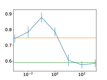
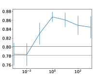
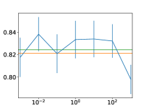
Annthyroid	Cardiotocography	InternetAds
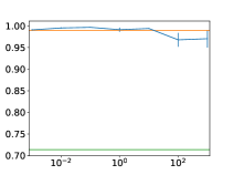
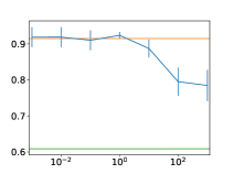
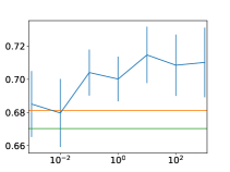
KDDCup99	PageBlocks	Pima
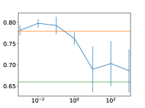
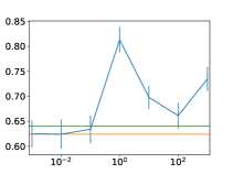
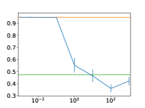
SpamBase	Waveform	Wilt

Figure 5: AUC by the proposed method with different hyperparameters $\lambda$ trained on data with ten inexact anomaly sets with five instances per set. The x-axis is hyperparameter $\lambda$ and the y-axis is AUC. Errorbar shows standard error. The green and orange horizontal lines are AUC by the proposed method with $\lambda=\infty$ and $\lambda=0$, respectively.

Figure 5 shows test AUC on the nine anomaly detection datasets by the proposed method with different hyperparameters $\lambda$. The best hyperparameters were different across datasets. For example, a high $\lambda$ was better with the Pima dataset, a low $\lambda$ was better with the PageBlocks and Wilt datasets, and an intermediate $\lambda$ was better with the Annthyroid and Waveform datasets. The proposed method achieved high performance with various datasets by automatically adapting $\lambda$ using the validation data to control the balance of the anomaly score minimization for non-anomalous instances and inexact AUC maximization.

6 Conclusion

We proposed an extension of the AUC for inexact labels, and developed a supervised anomaly detection method for data with inexact labels. With our proposed method, we trained a neural network-based anomaly score function by maximizing the inexact AUC while minimizing the anomaly scores for non-anomalous instances. We experimentally confirmed its effectiveness using various datasets. For future work, we would like to extend our framework for semi-supervised settings (Blanchard et al., 2010), where unlabeled instances, labeled anomalous and labeled non-anomalous instances are given for training.

References

- Akcay et al. (2018) S. Akcay, A. Atapour-Abarghouei, and T. P. Breckon. Ganomaly: Semi-supervised anomaly detection via adversarial training. In 14th Asian Conference on Computer Vision, 2018.
- Aleskerov et al. (1997) E. Aleskerov, B. Freisleben, and B. Rao. Cardwatch: A neural network based database mining system for credit card fraud detection. In IEEE/IAFE Computational Intelligence for Financial Engineering, pages 220–226, 1997.
- An and Cho (2015) J. An and S. Cho. Variational autoencoder based anomaly detection using reconstruction probability. Special Lecture on IE, 2:1–18, 2015.
- Andrews et al. (2003) S. Andrews, I. Tsochantaridis, and T. Hofmann. Support vector machines for multiple-instance learning. In Advances in Neural Information Processing Systems, pages 577–584, 2003.
- Babenko et al. (2009) B. Babenko, M.-H. Yang, and S. Belongie. Visual tracking with online multiple instance learning. In IEEE Conference on Computer Vision and Pattern Recognition, pages 983–990. IEEE, 2009.
- Blanchard et al. (2010) G. Blanchard, G. Lee, and C. Scott. Semi-supervised novelty detection. Journal of Machine Learning Research, 11(Nov):2973–3009, 2010.
- Brefeld and Scheffer (2005) U. Brefeld and T. Scheffer. AUC maximizing support vector learning. In Proceedings of the ICML Workshop on ROC Analysis in Machine Learning, 2005.
- Breiman (2001) L. Breiman. Random forests. Machine learning, 45(1):5–32, 2001.
- Breunig et al. (2000) M. M. Breunig, H.-P. Kriegel, R. T. Ng, and J. Sander. LOF: identifying density-based local outliers. ACM SIGMOD Record, 29(2):93–104, 2000.
- Campos et al. (2016) G. O. Campos, A. Zimek, J. Sander, R. J. Campello, B. Micenková, E. Schubert, I. Assent, and M. E. Houle. On the evaluation of unsupervised outlier detection: measures, datasets, and an empirical study. Data Mining and Knowledge Discovery, 30(4):891–927, 2016.
- Carbonneau et al. (2018) M.-A. Carbonneau, V. Cheplygina, E. Granger, and G. Gagnon. Multiple instance learning: A survey of problem characteristics and applications. Pattern Recognition, 77:329–353, 2018.
- Chandola et al. (2009) V. Chandola, A. Banerjee, and V. Kumar. Anomaly detection: A survey. ACM Computing Surveys, 41(3):15, 2009.
- Chong and Tay (2017) Y. S. Chong and Y. H. Tay. Abnormal event detection in videos using spatiotemporal autoencoder. In International Symposium on Neural Networks, pages 189–196. Springer, 2017.
- Cinbis et al. (2017) R. G. Cinbis, J. Verbeek, and C. Schmid. Weakly supervised object localization with multi-fold multiple instance learning. IEEE Transactions on Pattern Analysis and Machine Intelligence, 39(1):189–203, 2017.
- Cortes and Mohri (2004) C. Cortes and M. Mohri. AUC optimization vs. error rate minimization. In Advances in Neural Information Processing Systems, pages 313–320, 2004.
- Das et al. (2016) S. Das, W.-K. Wong, T. Dietterich, A. Fern, and A. Emmott. Incorporating expert feedback into active anomaly discovery. In 16th International Conference on Data Mining, pages 853–858. IEEE, 2016.
- Das et al. (2017) S. Das, W.-K. Wong, A. Fern, T. G. Dietterich, and M. A. Siddiqui. Incorporating feedback into tree-based anomaly detection. In KDD Workshop on Interactive Data Exploration and Analytics, 2017.
- Dietterich et al. (1997) T. G. Dietterich, R. H. Lathrop, and T. Lozano-Pérez. Solving the multiple instance problem with axis-parallel rectangles. Artificial intelligence, 89(1-2):31–71, 1997.
- Dodd and Pepe (2003) L. E. Dodd and M. S. Pepe. Partial AUC estimation and regression. Biometrics, 59(3):614–623, 2003.
- Dokas et al. (2002) P. Dokas, L. Ertoz, V. Kumar, A. Lazarevic, J. Srivastava, and P.-N. Tan. Data mining for network intrusion detection. In NSF Workshop on Next Generation Data Mining, pages 21–30, 2002.
- Eskin (2000) E. Eskin. Anomaly detection over noisy data using learned probability distributions. In International Conference on Machine Learning, 2000.
- Feng and Zhou (2017) J. Feng and Z.-H. Zhou. Deep miml network. In Thirty-First AAAI Conference on Artificial Intelligence, 2017.
- Fujimaki et al. (2005) R. Fujimaki, T. Yairi, and K. Machida. An approach to spacecraft anomaly detection problem using kernel feature space. In International Conference on Knowledge Discovery in Data Mining, pages 401–410, 2005.
- Fujino and Ueda (2016) A. Fujino and N. Ueda. A semi-supervised AUC optimization method with generative models. In 16th International Conference on Data Mining, pages 883–888. IEEE, 2016.
- Gao et al. (2006) J. Gao, H. Cheng, and P.-N. Tan. A novel framework for incorporating labeled examples into anomaly detection. In Proceedings of the 2006 SIAM International Conference on Data Mining, pages 594–598. SIAM, 2006.
- Hanley and McNeil (1982) J. A. Hanley and B. J. McNeil. The meaning and use of the area under a receiver operating characteristic (ROC) curve. Radiology, 143(1):29–36, 1982.
- Herrera et al. (2016) F. Herrera, S. Ventura, R. Bello, C. Cornelis, A. Zafra, D. Sánchez-Tarragó, and S. Vluymans. Multiple instance learning: foundations and algorithms. Springer, 2016.
- Hodge and Austin (2004) V. Hodge and J. Austin. A survey of outlier detection methodologies. Artificial Ntelligence Review, 22(2):85–126, 2004.
- Idé and Kashima (2004) T. Idé and H. Kashima. Eigenspace-based anomaly detection in computer systems. In International Conference on Knowledge Discovery and Data Mining, pages 440–449, 2004.
- Ilse et al. (2018) M. Ilse, J. Tomczak, and M. Welling. Attention-based deep multiple instance learning. In International Conference on Machine Learning, pages 2132–2141, 2018.
- Iwata and Yamanaka (2019) T. Iwata and Y. Yamanaka. Supervised anomaly detection based on deep autoregressive density estimators. arXiv preprint arXiv:1904.06034, 2019.
- Kingma and Ba (2015) D. P. Kingma and J. Ba. ADAM: A method for stochastic optimization. In International Conference on Learning Representations, 2015.
- Kingma and Wellniga (2014) D. P. Kingma and M. Wellniga. Auto-encoding variational Bayes. In 2nd International Conference on Learning Representations, 2014.
- Laxhammar et al. (2009) R. Laxhammar, G. Falkman, and E. Sviestins. Anomaly detection in sea traffic - a comparison of the Gaussian mixture model and the kernel density estimator. In International Conference on Information Fusion, pages 756–763, 2009.
- Liu et al. (2008) F. T. Liu, K. M. Ting, and Z.-H. Zhou. Isolation forest. In Proceeding of the 8th IEEE International Conference on Data Mining, pages 413–422. IEEE, 2008.
- Markou and Singh (2003) M. Markou and S. Singh. Novelty detection: a review. Signal processing, 83(12):2481–2497, 2003.
- Maron and Lozano-Pérez (1998) O. Maron and T. Lozano-Pérez. A framework for multiple-instance learning. In Advances in Neural Information Processing Systems, pages 570–576, 1998.
- Mukkamala et al. (2005) S. Mukkamala, A. Sung, and B. Ribeiro. Model selection for kernel based intrusion detection systems. In Adaptive and Natural Computing Algorithms, pages 458–461. Springer, 2005.
- Munawar et al. (2017) A. Munawar, P. Vinayavekhin, and G. De Magistris. Limiting the reconstruction capability of generative neural network using negative learning. In 27th International Workshop on Machine Learning for Signal Processing. IEEE, 2017.
- Nadeem et al. (2016) M. Nadeem, O. Marshall, S. Singh, X. Fang, and X. Yuan. Semi-supervised deep neural network for network intrusion detection. In KSU Conference on Cybersecurity Education, Research and Practice, 2016.
- Narasimhan and Agarwal (2017) H. Narasimhan and S. Agarwal. Support vector algorithms for optimizing the partial area under the ROC curve. Neural Computation, 29(7):1919–1963, 2017.
- Paszke et al. (2017) A. Paszke, S. Gross, S. Chintala, G. Chanan, E. Yang, Z. DeVito, Z. Lin, A. Desmaison, L. Antiga, and A. Lerer. Automatic differentiation in PyTorch. In NIPS Autodiff Workshop, 2017.
- Patcha and Park (2007) A. Patcha and J.-M. Park. An overview of anomaly detection techniques: Existing solutions and latest technological trends. Computer Networks, 51(12):3448–3470, 2007.
- Pedregosa et al. (2011) F. Pedregosa, G. Varoquaux, A. Gramfort, V. Michel, B. Thirion, O. Grisel, M. Blondel, P. Prettenhofer, R. Weiss, V. Dubourg, et al. Scikit-learn: Machine learning in python. Journal of Machine Learning Research, 12:2825–2830, 2011.
- Pimentel et al. (2018) T. Pimentel, M. Monteiro, J. Viana, A. Veloso, and N. Ziviani. A generalized active learning approach for unsupervised anomaly detection. arXiv preprint arXiv:1805.09411, 2018.
- Pinheiro and Collobert (2015) P. O. Pinheiro and R. Collobert. From image-level to pixel-level labeling with convolutional networks. In Proceedings of the IEEE Conference on Computer Vision and Pattern Recognition, pages 1713–1721, 2015.
- Rapaka et al. (2003) A. Rapaka, A. Novokhodko, and D. Wunsch. Intrusion detection using radial basis function network on sequences of system calls. In International Joint Conference on Neural Networks, volume 3, pages 1820–1825, 2003.
- Sabokrou et al. (2016) M. Sabokrou, M. Fathy, and M. Hoseini. Video anomaly detection and localisation based on the sparsity and reconstruction error of auto-encoder. Electronics Letters, 52(13):1122–1124, 2016.
- Sakai et al. (2018) T. Sakai, G. Niu, and M. Sugiyama. Semi-supervised AUC optimization based on positive-unlabeled learning. Machine Learning, 107(4):767–794, 2018.
- Sakurada and Yairi (2014) M. Sakurada and T. Yairi. Anomaly detection using autoencoders with nonlinear dimensionality reduction. In Proceedings of the MLSDA 2nd Workshop on Machine Learning for Sensory Data Analysis. ACM, 2014.
- Schölkopf et al. (2001) B. Schölkopf, J. C. Platt, J. Shawe-Taylor, A. J. Smola, and R. C. Williamson. Estimating the support of a high-dimensional distribution. Neural Computation, 13(7):1443–1471, 2001.
- Schölkopf et al. (2002) B. Schölkopf, A. J. Smola, et al. Learning with kernels: support vector machines, regularization, optimization, and beyond. MIT press, 2002.
- Shewhart (1931) W. A. Shewhart. Economic control of quality of manufactured product. ASQ Quality Press, 1931.
- Singh and Silakari (2009) S. Singh and S. Silakari. An ensemble approach for feature selection of cyber attack dataset. arXiv preprint arXiv:0912.1014, 2009.
- Suh et al. (2016) S. Suh, D. H. Chae, H.-G. Kang, and S. Choi. Echo-state conditional variational autoencoder for anomaly detection. In International Joint Conference on Neural Networks, pages 1015–1022, 2016.
- Wong et al. (2003) W.-K. Wong, A. W. Moore, G. F. Cooper, and M. M. Wagner. Bayesian network anomaly pattern detection for disease outbreaks. In International Conference on Machine Learning, pages 808–815, 2003.
- Wu et al. (2015) J. Wu, Y. Yu, C. Huang, and K. Yu. Deep multiple instance learning for image classification and auto-annotation. In Proceedings of the IEEE Conference on Computer Vision and Pattern Recognition, pages 3460–3469, 2015.
- Xu et al. (2018) H. Xu, W. Chen, N. Zhao, Z. Li, J. Bu, Z. Li, Y. Liu, Y. Zhao, D. Pei, Y. Feng, et al. Unsupervised anomaly detection via variational auto-encoder for seasonal kpis in web applications. In World Wide Web Conference, pages 187–196, 2018.
- Yamanishi et al. (2004) K. Yamanishi, J.-I. Takeuchi, G. Williams, and P. Milne. On-line unsupervised outlier detection using finite mixtures with discounting learning algorithms. Data Mining and Knowledge Discovery, 8(3):275–300, 2004.
- Ying et al. (2016) Y. Ying, L. Wen, and S. Lyu. Stochastic online AUC maximization. In Advances in Neural Information Processing Systems, pages 451–459, 2016.
- Zhai et al. (2016) S. Zhai, Y. Cheng, W. Lu, and Z. Zhang. Deep structured energy based models for anomaly detection. In International Conference on Machine Learning, pages 1100–1109, 2016.
- Zhou and Paffenroth (2017) C. Zhou and R. C. Paffenroth. Anomaly detection with robust deep autoencoders. In Proceedings of the 23rd ACM SIGKDD International Conference on Knowledge Discovery and Data Mining, pages 665–674. ACM, 2017.
- Zhu et al. (2017) W. Zhu, Q. Lou, Y. S. Vang, and X. Xie. Deep multi-instance networks with sparse label assignment for whole mammogram classification. In International Conference on Medical Image Computing and Computer-Assisted Intervention, pages 603–611, 2017.