The real and imaginary parts of a weak value appearing as back-actions via a post-selection

Abstract

In a weak measurement the real and imaginary parts of a weak value participate in the shifts of the complementary variables of a pointer. While the real part represents the value of an observable in the limit of zero measurement strength, the imaginary one is regarded as the back-action due to the measurement with a post-selection, which has an influence on the post-selection probability. In this paper I give a case in which a real part could also appear as such a back-action in a post-selection probability on an equal footing with an imaginary one. It is also shown that both of the real and imaginary parts can be inferred by observing the probability in practice, which has an advantage that an additional system of a pointer is not needed.

I Introduction

Recently a weak value has attracted attention in both of the foundation and the application of quantum mechanics. The value was originally introduced as a result of a weak measurement Aharonov et al. (1988), which gives us a value of an observable, $\hat{O}$, as an ensemble average without disturbing the measured system. When the system is initially in $|\psi\rangle$ (pre-selection), and is finally found in $|\phi\rangle$ (post-selection), a weak measurement performed between the pre-post-selection shows the weak value of $\hat{O}$ as follows,

$$\langle\hat{O}\rangle_{\bf w}=\langle\phi|\hat{O}|\psi\rangle/\langle\phi|\psi\rangle.$$ (1)

Although a pre-post-selection has been often seen as in quantum information processing, the concept of a weal value was inspired by a time symmetric description of quantum mechanics Aharonov et al. (1964); Aharonov and Vaidman (1991). Actually a weak measurement has offered a new approach to the foundation of quantum mechanics, for example, in the Leggett-Garg inequality Williams and Jordan (2008); Dressel et al. (2011); Goggin et al. (2011), the contextuality Tollaksen (2007); Pusey (2014); Piacentini et al. (2016); Waegell et al. (2017); Kunjwal et al. (2018) and so on, since we can access a quantum system without disturbance. In particular a weak measurement has been performed experimentally for observation of a quantum paradox Aharonov and Vaidman (1991); Resch et al. (2004); Aharonov et al. (2002); Lundeen and Steinberg (2009); Yokota et al. (2009); Vaidman (2013); Danan et al. (2013); Aharonov et al. (2013); Denkmayr et al. (2014); Aharonov et al. (2016, 2017); Elitzur et al. (2018). It has been also shown that a weak value itself plays an important role in a quantum phenomenon irrespective of a weak measurement Steinberg (1995a); Rohrlich and Aharonov (2002); Yokota and Imoto (2012, 2014).

The large shift of a pointer could be produced in a weak measurement by choosing a pre-post-selection on purpose as $\langle\phi|\psi\rangle\rightarrow 0$ in equation (1). Using such an amplification effect, an application for precision measurement has been actually demonstrated Hosten and Kwiat (2008); Dixon et al. (2009); Hallaji et al. (2017); Lee and Tsutsui (2014); Ferrie and Combes (2014); Jordan et al. (2014); Knee and Gauger (2014); Mori et al. (2019). As another application, a weak measurement has been also expected in sensing science Howland et al. (2014); Mirhosseini et al. (2014) beyond the fundamental issue of direct measurement of a quantum state Lundeen et al. (2011); Kocsis et al. (2011).

According to the definition in equation (1), a weak value is generally a complex number. In a weak measurement the real and imaginary parts of a weak value appear as the shifts in the complementary variables of a pointer: For example, the position of the pointer, $x$, shifts in response to the real part, while the imaginary one participates in the shift of the momentum, $p$ ($[x,p]=i\hbar$).

Despite of such a similarity the interpretation of each parts has been actively discussed: While the real part has been naively considered as the value of the measured observable in the limit of zero disturbance, the imaginary one seems to represent the disturbance (back-action) due to the measurement with a postselection Dressel and Jordan (2012); Steinberg (1995b); Aharonov and Botero (2005).

Roughly speaking, the real part of a weak value has mostly played a significant role in a fundamental issue as in a quantum paradox so far. On the other hand, an imaginary part has been found to be practically useful in the application of an amplification for precision measurement Brunner and Simon (2010); Kedem (2012), while recently it was reported that an appearance of an imaginary part can be associated with contextuality Kunjwal et al. (2018).

In this paper I show a case that the real part of a weak value also could have an influence on the post-selection probability as a back-action in the same manner as the imaginary one. While I expect such a suggestion to open up a new approach for deeper understanding of a weak value as trying to treat both of the parts on an equal footing, I would like to discuss an application for estimating a weak value experimentally on this occasion: Without preparing an additional system of a measurement apparatus, both of the real and imaginary parts can be inferred by observing the post-selection probability affected by their back-actions.

II The real and imaginary parts of a weak value in a weak measurement

First I would like to review a weak measurement by using von Neumann measurement model as originally proposed in Aharonov et al. (1988), and introduce the real and imaginary parts of a weak value.

A measurement apparatus is prepared as in the state of $|\Psi(Q)\rangle$, where $Q$ represents the position of a pointer which gives us a result of measurement. I assume the distribution of the position is provided by a Gaussian function as follows,

$$\langle Q|\Psi(Q)\rangle={\rm exp}\bigg{(}-\frac{Q^{2}}{2\sigma^{2}}\bigg{)}$$ (2)

up to normalization, where $\sigma^{2}$ presents the variance. To observe $\hat{O}$ on a quantum system, $|\psi\rangle$, the system is interacted with the pointer by the interacting Hamiltonian as follows,

$$\hat{H}=g(t)\hat{O}\hat{P},$$ (3)

with the momentum of the pointer, $\hat{P}$; the coupling function, $g(t)$, satisfying $\int dtg(t)=G$ for the duration of the interaction. As a result the system is correlated with the pointer as follows,

$$|\psi\rangle\otimes|\Psi(Q)\rangle\rightarrow\sum_{k}\langle o_{k}|\psi\rangle|o_{k}\rangle\otimes|\Psi(Q-Go_{k})\rangle,$$ (4)

where I have assumed $\hat{O}$ has the discrete spectrum of an eigenvalue, $o_{k}$, with an eigenstate of $|o_{k}\rangle$.

The coupling strength can be controlled by $G$, which corresponds to the measurement strength. Actually, when $G$ is large enough, we can certainly discriminate which eigenstate the system is in by reading the shift of the pointer in response to the eigenvalue, $\Delta Q=Go_{k}$. Then the system is utterly disturbed by the measurement, as the system results in one of the eigenstates, $|o_{k}\rangle$. As such an observation of the eigenstate appears with a probability, $|\langle o_{k}|\psi\rangle|^{2}$, the average of the pointer shift gives us the ensemble average, $\bar{O}=\langle\psi|\hat{O}|\psi\rangle$. In this case the measurement model well represents a conventional measurement process, which is so-called a strong measurement.

On the other hand, given $\sigma$, a weak measurement is achieved in $G\rightarrow 0$. The system is not disturbed due to the almost no correlation, which seems a failure of measurement. Even in this case, however, the pointer contains a piece of information on the system. Actually, if the ensemble average is taken, the probability distribution of the pointer position is given by $Prob(Q)\sim|\Psi(Q-G\bar{O})|^{2}$. Unlike a strong measurement, the ensemble average, $\bar{O}$, is obtained without disturbance on the system.

Furthermore, when the system is finally post-selected in $|\phi\rangle$, the shift of the pointer is given by the weak value as follows,

$$\langle\phi|e^{-\frac{i}{\hbar}G\hat{O}\hat{P}}|\psi\rangle\otimes|\Psi(Q)\rangle$$ (5)

$$\sim \langle\phi|(1-\frac{i}{\hbar}G\hat{O}\hat{P})|\psi\rangle\otimes|\Psi(Q)\rangle$$

$$\sim \langle\phi|\psi\rangle e^{-\frac{i}{\hbar}G\langle\hat{O}\rangle_{\bf w}\hat{P}}|\Psi(Q)\rangle.$$

As shown in equation (1), the weak value is generally a complex number; The real and imaginary parts of the weak value appear in the shifts of the position, $\Delta Q=G{\rm Re}\langle\hat{O}\rangle_{\bf w}$, and the momentum, $\Delta P=2G{\rm Im}\langle\hat{O}\rangle_{\bf w}/\sigma^{2}$, respectively Jozsa (2007). Then, as in the case of a conventional strong measurement, the real part is simply obtained by the shift of the position, $\Delta Q$, normalized by the measurement strength, $G$, i.e. $\Delta Q/G$. On the imaginary part, the momentum shift contains the variance of the pointer $\sigma^{2}$ unlike the real one.

Actually, without reference to von Neumann measurement model, it has been known that the shift corresponding to the imaginary part depends on the details of the pointer. As a result it gives rise to the different interpretations of the real and imaginary parts of a weak value. While the real part can be regarded as the conditioned average of $\hat{O}$ in the limit of zero disturbance, the imaginary one can not be naively associated with the measurement of $\hat{O}$; Rather the imaginary part is interpreted as disturbance (back-action) Dressel and Jordan (2012), which could be confirmed in the success probability of the post-selection as discussed in the next section.

III A weak value appearing as a back-action via a post-selection

In Dressel and Jordan (2012) it was clarified what the imaginary part of a weak value represents in a weak measurement: An imaginary part provides information about how the initial state is disturbed by the observable operator, which could be confirmed in the change of post-selection probability.

To see this, I re-describe the Hamiltonian of equation (3) with $\int dtg(t)\hat{P}/\hbar=G\hat{P}/\hbar\equiv\theta$ as in Kedem (2014) without referring to a pointer. As the momentum, $P$, is a constant of motion under the Hamiltonian, I have regarded $\theta$ as just a parameter. Then the post-selection probability is given as follows,

$$Prob(\phi) = |\langle\phi|e^{-i\theta\hat{O}}|\psi\rangle|^{2}$$ (6)

$$\sim |\langle\phi|\psi\rangle|^{2}(1+2\theta{\rm Im}\langle\hat{O}\rangle_{\bf w}),$$

in $\theta<<1$ corresponding to weak measurement. I refer to the change of the post-selection probability due to the weak value as ‘back-action.’ In fact I will show that such a back-action in the post-selection probability could be also come into by not only the imaginary part of a weak value but also the real part.

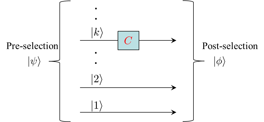
Figure 1: A photon takes the superposition of the path state, $|k\rangle$, which is pre-post-selected in $|\psi\rangle$ and $|\phi\rangle$.

When deriving equation (6), I have payed attention to only the measured system. Actually the back-action given by a weak value does not need to rely on the context of a weak measurement any longer. To clarify this point, it will be helpful to treat a specific case of a photon.

Suppose that a photon can take paths, $\{|k\rangle\}$, and the initial state is in the superposition as follows,

$$|\psi\rangle=\sum_{k}\langle k|\psi\rangle|k\rangle.$$ (7)

Additionally the path state is finally post-selected in $|\phi\rangle$, and I would like to discuss one of the weak values of the projectors, $|k\rangle\langle k|$. As shown in figure 1, an optical component is placed on the path, $|k\rangle$, by which the corresponding term is multiplied by a c-number, $C$: $|k\rangle\rightarrow C|k\rangle$.

In this case the back-action in the post-selection probability in equation (6) can be imitated by setting the phase shifter, $C=e^{-i\theta}$, on the path of $|k\rangle$: the probability changes as follows,

$$Prob(\phi) = |\langle\phi|e^{-i\theta}|k\rangle\langle k|\psi\rangle|^{2}$$ (8)

$$\sim |\langle\phi|\psi\rangle|^{2}(1+2\theta{\rm Im}\langle|k\rangle\langle k|\rangle_{\bf w}),$$

in $\theta<<1$.

On the other hand, when the optical component is an attenuator with the transmittance, $T=1-R$, i.e. $C=\sqrt{T}\equiv e^{-\alpha}$ ($\alpha\geq 0$), the post-selection probability is given as follows,

$$Prob(\phi) = |\langle\phi|e^{-\alpha}|k\rangle\langle k|\psi\rangle|^{2}$$ (9)

$$\sim |\langle\phi|\psi\rangle|^{2}(1-2\alpha{\rm Re}\langle|k\rangle\langle k|\rangle_{\bf w})$$ (10)

$$\sim |\langle\phi|\psi\rangle|^{2}(1-R{\rm Re}\langle|k\rangle\langle k|\rangle_{\bf w}),$$ (11)

where I have assumed $\alpha<<1$ ($R<<1$).

Generally when a c-number, $C_{k}$, is applied to the path, $|k\rangle$, the post-selection probability is given as follows,

$$Prob(\phi)=|\langle\phi|\psi\rangle|^{2}\bigg{|}\sum_{k}C_{k}\langle|k\rangle\langle k|\rangle_{\bf w}\bigg{|}^{2};$$ (12)

If $C_{k}$ satisfies the condition of a weak disturbance like $\theta,\alpha<<1$, a weak value of each path explicitly appears as in equations (8) and (10).

In Yokota and Imoto (2018a) it was already shown that a real weak value is useful in estimating how the post-selection probability is change by dissipations which are placed between the pre-post-selection: A negative real weak value well represents a negation of a dissipation against a positive one. Especially, when $\langle|k\rangle\langle k|\rangle_{\bf w}=1$ in equation (9) without the approximation, the post-selection probability decreases as if a photon has passed the attenuator with certainty, i.e. $Prob(\phi)=T|\langle\phi|\psi\rangle|^{2}$. In addition the same attenuator is added on another path of $\langle|k^{\prime}\rangle\langle k^{\prime}|\rangle_{\bf w}=-1$, the probability restores to $|\langle\phi|\psi\rangle|^{2}$, according to equation (12).

In this discussion of Yokota and Imoto (2018a), the negative weak value of $-1$ by itself does not make sense, since the negative value cannot be related to ‘negation’ without the positive value. In other words the negative weak value of $-1$ is meaningful in the equation, $1-1=0$.

However, under the weak condition of $R<<1$ in equation (11), the negative weak value itself can be a counterpart of the positive weak value: While the positive weak value of $1$ gives the post-selection probability of $Prob(\phi)=(1-R)|\langle\phi|\psi\rangle|^{2}$, the negative value of $-1$ gives the probability, $Prob(\phi)=(1+R)|\langle\phi|\psi\rangle|^{2}$. Although such a symmetric relation of the positive weak value $1$ and the negative one $-1$ was also confirmed as linear-polarization shift in Yokota and Imoto (2016), I have shown that the symmetric relation is also found in the post-selection probability without another system of polarization. Actually the supplementary result of Figure.5(b) in Yokota and Imoto (2018a) implies such a symmetric relation when $T$ is large (i.e. $R<<1$).

Another point to note is when the component on the path of $|k\rangle$ provides a c-number, $C=e^{-\alpha}e^{-i\theta}$. In this case the probability is simply given by

$$Prob(\phi)\sim|\langle\phi|\psi\rangle|^{2}(1+2\theta{\rm Im}\langle|k\rangle\langle k|\rangle_{\bf w}$$

$$\ \ \ \ \ \ \ \ \ \ \ \ \ \ \ \ \ \ \ \ \ \ \ \ \ \ \ \ -2\alpha{\rm Re}\langle|k\rangle\langle k|\rangle_{\bf w}),$$ (13)

with $\theta,\alpha$ $<<1$. Both of the real and imaginary parts of a weak value appear in an equal footing. Clearly such equivalent contributions to the post-selection probability by both of the parts are also found in another situation, for example, when components are set on some paths (not only on one path). As shown in equation (12), the c-number on each path is weighted by the corresponding weak value. Under the weak condition ($\theta,\alpha<<1$), the real and imaginary parts of a c-number are weighted by the real and imaginary parts of the corresponding weak value respectively.

IV An application of the back-action by a weak value

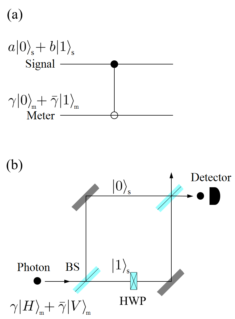
Figure 2: (a)A CNOT operation for a weak measurement on a qubit. The signal qubit is correlated with the meter qubit, whose strength is controlled by the input state of the meter, namely $\gamma$ and $\bar{\gamma}$. (b)A weak measurement on the path state of a photon, $\langle|1\rangle_{s}\langle 1|\rangle_{\bf w}$ and $1-\langle|1\rangle_{s}\langle 1|\rangle_{\bf w}=\langle|0\rangle_{s}\langle 0|\rangle_{\bf w}$. The pre-post-selection on the path state is accomplished by the interferometer composed of the beam splitters (BS) and the detection of one of the output ports. The horizontal (vertical) polarization, $|H\rangle_{m}$ ($|V\rangle_{m}$) corresponds to $|0\rangle_{m}$ ($|1\rangle_{m}$) of the meter qubit. The CNOT operation is achieved by the half wave plate (HWP), by which the polarization is changed as $|H\rangle_{m}\leftrightarrow|V\rangle_{m}$.

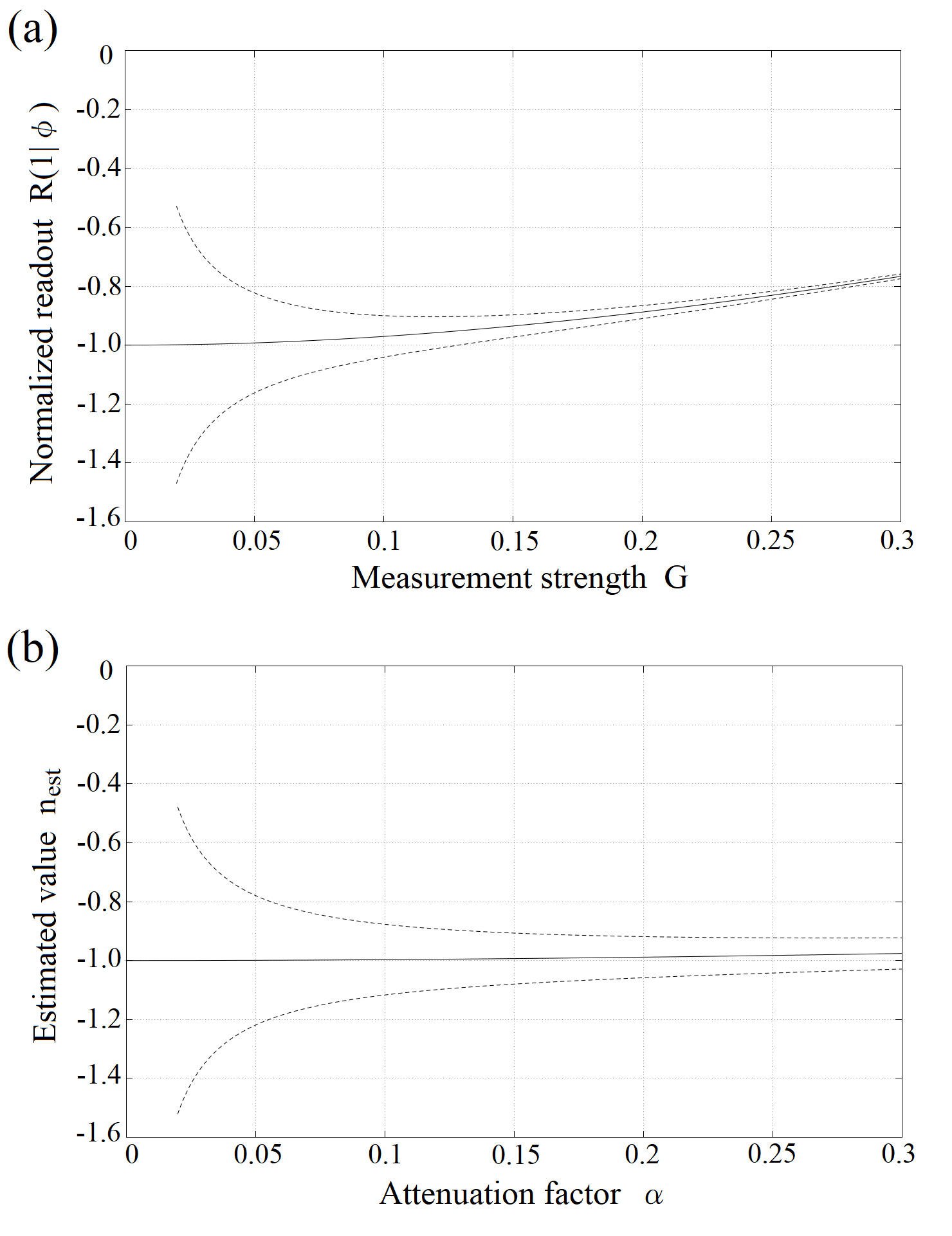
Figure 3: (a)The normalized readout. (b)The estimated value from the post-selection probability. In the limit of the measurement strength $G$ $\rightarrow$ $0$ and the attenuation factor $\alpha$ $\rightarrow$ $0$, they show the real part of a weak value, $-1$. The solid lines correspond to the ideal values of equation (14) and (16), while the dashed lines represent the errors stemming from the Poisson statistics of the photon counts: the photon counts of the post-selection, $|\langle\phi|\psi\rangle|^{2}$, is assumed to be $10000$, based on which the other counts are considered to calculate the probabilities, $Prob(1|\phi)$ and $Prob(\phi)$.

I have shown that both of the real and imaginary parts of a weak value could contribute to the post-selection probability. In this section I would like to discuss an application of this result, that is, whether it is practical to estimate both of the parts by observing the post-selection probability in equations (8) and (10).

For experimentally observing a weak value, it is straightforward to use a weak measurement as reading the pointer shift in equation (5). There are also experimental approaches to measure the real and imaginary weak values simultaneously Kobayashi et al. (2014); Hariri et al. (2019). Significantly a recent work has clarified a weak measurement is not always a good strategy in estimating a weak value: Rather a strong measurement can be efficient to determine a weak value experimentally Vallone and Dequal (2016); Cohen and Pollak (2018). Nonetheless, for an experimental verification of a fundamental issue like observation of a quantum paradox, it would be essential to perform measurement without disturbance on the quantum system.

In the previous case of the path state of a photon, a weak measurement on a qubit system is available (i.e. which-way measurement, $|k\rangle\langle k|$ or $1-|k\rangle\langle k|$). Actually it has been known that a CNOT operation with another qubit of a meter (measurement apparatus) achieves a weak measurement Pryde et al. (2005) as shown in figure 2(a). The qubit to be measured (signal) in $a|0\rangle_{s}+b|1\rangle_{s}$ is correlated with the meter qubit in $\gamma|0\rangle_{m}+\bar{\gamma}|1\rangle_{m}$ ($\gamma\geq\bar{\gamma}\geq 0$) by the CNOT, which results in $(a\gamma|0\rangle_{s}+b\bar{\gamma}|1\rangle_{s})|0\rangle_{m}+(a\bar{\gamma}|0\rangle_{s}+b\gamma|1\rangle_{s})|1\rangle_{m}$. The correlation strength (measurement strength) is represented by $G=\gamma^{2}-\bar{\gamma}^{2}$ ($0\leq G\leq 1$).

In this setup the normalized readout, $R(1|\phi)$, corresponding to the pointer of the measurement apparatus, gives the weak value as follows,

$$R(1|\phi) = \frac{Prob(1|\phi)-\bar{\gamma}^{2}}{G},$$ (14)

$$\rightarrow {\rm Re}\langle|1\rangle\langle 1|\rangle_{\bf w}\ (G\rightarrow 0),$$ (15)

where $Prob(1|\phi)$ represents the probability of observing the meter as $|1\rangle_{m}$ under the success of the post-selection, $|\phi\rangle_{s}$. Actually a polarization has been often used as the meter for a weak measurement on the path state of a photon Yokota et al. (2009); Yokota and Imoto (2018a, 2016) as shown in figure 2 (b).

On the other hand, the estimation of a weak value from the post-selection probability, equations (8) and (10), has an advantage that we need not prepare an ancilla system to play a role of a meter; As mentioned later, saving the physical resource will be beneficial in a joint weak measurement. It also achieves no disturbance in the limit of $\theta,\alpha\rightarrow 0$, albeit such an inference of a weak value is different from a weak measurement straightforwardly.

For example, according to equation (10), the real part of a weak value can be inferred as follows,

$$n_{\rm est} = \frac{1}{2\alpha}\bigg{(}1-\frac{Prob(\phi)}{|\langle\phi|\psi\rangle|^{2}}\bigg{)}$$ (16)

$$\rightarrow {\rm Re}\langle|1\rangle\langle 1|\rangle_{\bf w}\ (\alpha\rightarrow 0).$$ (17)

So as to show the above estimation is comparable to a weak measurement in practice, I calculated equations (14) and (16) when a weak value is $\langle|k\rangle\langle k|\rangle_{\bf w}=-1$ for the path state of a photon as shown in figure 3 (a) and (b) respectively. Clearly the inference of a weak value from the post-selection probability is adequate for practical use.

A weak value in the system more than 2 qubits is called a joint weak value, say $\langle|kl\rangle\langle kl|\rangle_{\bf w}$. It is known that a joint weak value can be estimated from a correlation of pointers in the higher order on the measurement strength like $G^{2}$ Lundeen and Steinberg (2009); Resch and Steinberg (2004); Kobayashi et al. (2012); Kumari et al. (2017). Be that as it may, to perform a joint weak measurement straightforwardly, entangled meter qubits are generally needed Yokota et al. (2009); Yokota and Imoto (2018b) as long as considering local operations, where ‘local’ means a signal qubit is interacted with only the corresponding meter qubit (not the other meter qubits).

However such an entangled meter is not needed in inferring a weak value from the post-selection probability; Alternatively the c-number acts on only the corresponding term: $|kl\rangle\rightarrow C|kl\rangle$. For example, the polarization can be free for a signal qubit in the case of a photon in figure 2 (b). Then it will practically be easy to perform an experiment involving a joint weak value by using such hybrid signals (the path and the polarization) of a single photon with experimental determination of the joint weak value.

V Summary

The characteristic of the imaginary part of a weak value has been regarded as be different from the one of the real part, especially, in the context of a weak measurement. However I have shown that the real and imaginary parts could appear in an equal footing as the back-action in a post-selection probability. By observing the post-selection probability, both of the real and imaginary parts can be experimentally inferred in the limit of no disturbance on the system. Such an estimation of a weak value has an advantage because of saving an additional system of a measurement apparatus. Actually the back-action itself have no direct relation to weak measurement: In my discussion just an optical component to provide a c-number has been assumed, which has no observable variables to show some result of measurement, namely, a pointer. It relies on a weak value how the component participates in the post-selection probability.

Besides an application of estimating a weak value, I also expect that the significance of a weak value will be more clarified: Since the real and imaginary parts could be discussed in an equal footing, the imaginary one could serve with newfound reality, as a real one has been an affinity to a probability.

References

- Aharonov et al. (1988) Y. Aharonov, D. Z. Albert, and L. Vaidman, “How the result of a measurement of a component of the spin of a spin-1/2 particle can turn out to be 100,” Phys. Rev. Lett. 60, 1351 (1988).
- Aharonov et al. (1964) Y. Aharonov, P. G. Bergmann, and J. L. Lebowitz, “Time symmetry in the quantum process of measurement,” Phys. Rev. 134, B1410 (1964).
- Aharonov and Vaidman (1991) Y. Aharonov and L. Vaidman, “Complete description of a quantum system at a given time,” J. Phys. A: Math. Gen. 24, 2315 (1991).
- Williams and Jordan (2008) N. S. Williams and A. N. Jordan, “Weak values and the leggett-garg inequality in solid-state qubits,” Phys. Rev. Lett. 100, 026804 (2008).
- Dressel et al. (2011) J. Dressel, C. J. Broadbent, J. C. Howell, and A. N. Jordan, “Experimental violation of two-party leggett-garg inequalities with semiweak measurements,” Phys. Rev. Lett. 106, 040402 (2011).
- Goggin et al. (2011) M. E. Goggin, M. P. Almeida, M. Barbieri, B. P. Lanyon, J. L. O’Brien, A. G. White, and G. J. Pryde, “Violation of the leggett-garg inequality with weak measurements of photons,” Proc. Natl. Acad. Sci. USA 108, 1256 (2011).
- Tollaksen (2007) J. Tollaksen, “Pre- and post-selection, weak values and contextuality,” J. Phys. A: Math. Theor. 40, 9033 (2007).
- Pusey (2014) M. F. Pusey, “Anomalous weak values are proofs of contextuality,” Phys. Rev. Lett. 113, 200401 (2014).
- Piacentini et al. (2016) F. Piacentini, A. Avella, M. P. Levi, R. Lussana, F. Villa, A. Tosi, F. Zappa, M. Gramegna, G. Brida, I. P. Degiovanni, and M. Genovese, “Experiment investigating the connection between weak values and contextuality,” Phys. Rev. Lett. 116, 180401 (2016).
- Waegell et al. (2017) M. Waegell, T. Denkmayr, H. Geppert, D. Ebner, T. Jenke, Y. Hasegawa, S. Sponar, J. Dressel, and J. Tollaksen, “Confined contextuality in neutron interferometry: Observing the quantum pigeonhole effect,” Phys. Rev. A 96, 052131 (2017).
- Kunjwal et al. (2018) R. Kunjwal, M. Lostaglio, and M. F. Pusey, “Anomalous weak values and contextuality: robustness, tightness, and imaginary parts,” arXiv:1812.06940 (2018).
- Resch et al. (2004) K. J. Resch, J. S. Lundeen, and A. M. Steinberg, “Experimental realization of the quantum box problem,” Phys. Lett. A 324, 125 (2004).
- Aharonov et al. (2002) Y. Aharonov, A. Botero, S. Popescu, B. Reznik, and J. Tollaksen, “Revisiting hardy’s paradox: counterfactual statements, real measurements, entanglement and weak values,” Phys. Lett. A 301, 130 (2002).
- Lundeen and Steinberg (2009) J. S. Lundeen and A. M. Steinberg, “Experimental joint weak measurement on a photon pair as a probe of hardy’s paradox,” Phys. Rev. Lett. 102, 020404 (2009).
- Yokota et al. (2009) K. Yokota, T. Yamamoto, M. Koashi, and N. Imoto, “Direct observation of hardy’s paradox by joint weak measurement with an entangled photon pair,” New J. Phys. 11, 033011 (2009).
- Vaidman (2013) L. Vaidman, “Past of a quantum particle,” Phys. Rev. A 87, 052104 (2013).
- Danan et al. (2013) A. Danan, D. Farfurnik, S. Bar-Ad, and L. Vaidman, “Asking photons where they have been,” Phys. Rev. Lett. 111, 240402 (2013).
- Aharonov et al. (2013) Y. Aharonov, S. Popescu, D. Rohrlich, and P. Skrzypczyk, “Quantum cheshire cats,” New J. Phys. 15, 113015 (2013).
- Denkmayr et al. (2014) T. Denkmayr, H. Geppert, S. Sponar, H. Lemmel, A. Matzkin, J. Tollaksen, and Y. Hasegawa, “Observation of a quantum cheshire cat in a matter-wave interferometer experiment,” Nat. Commun. 5, 4492 (2014).
- Aharonov et al. (2016) Y. Aharonov, F. Colombo, S. Popescu, I. Sabadini, D. C. Struppa, and J. Tollaksen, “Quantum violation of the pigeonhole principle and the nature of quantum correlations,” Proc. Natl. Acad. Sci. USA 113, 532 (2016).
- Aharonov et al. (2017) Y. Aharonov, E. Cohen, A. Landau, and A. C. Elitzur, “The case of the disappearing (and re-appearing) particle,” Sci. Rep. 7, 531 (2017).
- Elitzur et al. (2018) A. C. Elitzur, E. Cohen, R. Okamoto, and S. Takeuchi, “Nonlocal position changes of a photon revealed by quantum routers,” Sci. Rep. 8, 7730 (2018).
- Steinberg (1995a) A. M. Steinberg, “How much time does a tunneling particle spend in the barrier region?” Phys. Rev. Lett. 74, 2405 (1995a).
- Rohrlich and Aharonov (2002) D. Rohrlich and Y. Aharonov, “Cherenkov radiation of superluminal particles,” Phys. Rev. A 66, 042102 (2002).
- Yokota and Imoto (2012) K. Yokota and N. Imoto, “A strange weak value in spontaneous pair productions via a supercritical step potential,” New J. Phys. 14, 083021 (2012).
- Yokota and Imoto (2014) K. Yokota and N. Imoto, “A weak-value model for virtual particles supplying the electric current in graphene: the minimal conductivity and the schwinger mechanism,” New J. Phys. 16, 073003 (2014).
- Hosten and Kwiat (2008) O. Hosten and P. Kwiat, “Observation of the spin hall effect of light via weak measurements,” Science 319, 787 (2008).
- Dixon et al. (2009) P. B. Dixon, D. J. Starling, A. N. Jordan, and J. C. Howell, “Ultrasensitive beam deflection measurement via interferometric weak value amplification,” Phys. Rev. Lett. 102, 173601 (2009).
- Hallaji et al. (2017) M. Hallaji, A. Feizpour, G. Dmochowski, J. Sinclair, and A. M. Steinberg, “Weak-value amplification of the nonlinear effect of a single photon,” Nat. Phys. 13, 540 (2017).
- Lee and Tsutsui (2014) J. Lee and I. Tsutsui, “Merit of amplification by weak measurement in view of measurement uncertainty,” Quantum Stud.: Math. Found. 1, 65 (2014).
- Ferrie and Combes (2014) C. Ferrie and J. Combes, “Weak value amplification is suboptimal for estimation and detection,” Phys. Rev. Lett. 112, 040406 (2014).
- Jordan et al. (2014) A. N. Jordan, J. Martínez-Rincón, and J. C. Howell, “Technical advantages for weak-value amplification: When less is more,” Phys. Rev. X 4, 011031 (2014).
- Knee and Gauger (2014) G. C. Knee and E. M. Gauger, “When amplification with weak values fails to suppress technical noise,” Phys. Rev. X 4, 011032 (2014).
- Mori et al. (2019) Y. Mori, J. Lee, and I. Tsutsui, “On the validity of weak measurement applied for precision measurement,” arXiv:1901.06831 (2019).
- Howland et al. (2014) G. A. Howland, D. J. Lum, and J. C. Howell, “Compressive wavefront sensing with weak values,” Opt. Express 22, 18870 (2014).
- Mirhosseini et al. (2014) M. Mirhosseini, O. S. Magaa-Loaiza, S. M. H. Rafsanjani, and R. W. Boyd, “Compressive direct measurement of the quantum wave function,” Phys. Rev. Lett. 113, 090402 (2014).
- Lundeen et al. (2011) J. S. Lundeen, B. Sutherland, A. Patel, C. Stewart, and C. Bamber, “Direct measurement of the quantum wavefunction,” Nature 474, 188 (2011).
- Kocsis et al. (2011) S. Kocsis, B. Braverman, S. Ravets, M. J. Stevens, R. P. Mirin, L. K. Shalm, and A. M. Steinberg, “Observing the average trajectories of single photons in a two-slit interferometer,” Science 332, 1170 (2011).
- Dressel and Jordan (2012) J. Dressel and A. N. Jordan, “Significance of the imaginary part of the weak value,” Phys. Rev. A 85, 012107 (2012).
- Steinberg (1995b) A. M. Steinberg, “Conditional probabilities in quantum theory and the tunneling-time controversy,” Phys. Rev. A 52, 32 (1995b).
- Aharonov and Botero (2005) Y. Aharonov and A. Botero, “Quantum averages of weak values,” Phys. Rev. A 72, 052111 (2005).
- Brunner and Simon (2010) N. Brunner and C. Simon, “Measuring small longitudinal phase shifts: Weak measurements or standard interferometry?” Phys. Rev. Lett. 105, 010405 (2010).
- Kedem (2012) Y. Kedem, “Using technical noise to increase the signal-to-noise ratio of measurements via imaginary weak values,” Phys. Rev. A 85, 060102(R) (2012).
- Jozsa (2007) R. Jozsa, “Complex weak values in quantum measurement,” Phys. Rev. A 76, 044103 (2007).
- Kedem (2014) Y. Kedem, “Obtaining imaginary weak values with a classical apparatus: Applications for the time and frequency domains,” Phys. Lett. A 378, 2096 (2014).
- Yokota and Imoto (2018a) K. Yokota and N. Imoto, “Negation of photon loss provided by negative weak value,” J. Phys. Commun. 2, 065013 (2018a).
- Yokota and Imoto (2016) K. Yokota and N. Imoto, “When a negative weak value -1 plays the counterpart of a probability 1,” New J. Phys. 18, 123002 (2016).
- Kobayashi et al. (2014) H. Kobayashi, K. Nonaka, and Y. Shikano, “Stereographical visualization of a polarization state using weak measurements with an optical-vortex beam,” Phys. Rev. A 89, 053816 (2014).
- Hariri et al. (2019) A. Hariri, D. Curic, L. Giner, and J. S. Lundeen, “Experimental simultaneous read out of the real and imaginary parts of the weak value,” arXiv:1906.02263 (2019).
- Vallone and Dequal (2016) G. Vallone and D. Dequal, “Strong measurements give a better direct measurement of the quantum wave function,” Phys. Rev. Lett. 116, 040502 (2016).
- Cohen and Pollak (2018) E. Cohen and E. Pollak, “Determination of weak values of quantum operators using only strong measurements,” Phys. Rev. A 98, 042112 (2018).
- Pryde et al. (2005) G. J. Pryde, J. L. O’Brien, A. G. White, T. C. Ralph, and H. M. Wiseman, “Measurement of quantum weak values of photon polarizatoin,” Phys. Rev. Lett. 94, 220405 (2005).
- Resch and Steinberg (2004) K. J. Resch and A. M. Steinberg, “Extracting joint weak values with local, single-particle measurements,” Phys. Rev. Lett. 92, 130402 (2004).
- Kobayashi et al. (2012) H. Kobayashi, G. Puentes, and Y. Shikano, “Extracting joint weak values from two-dimensional spatial displacements,” Phys. Rev. A 86, 053805 (2012).
- Kumari et al. (2017) A. Kumari, A. K. Pan, and P. K. Panigrahi, “Joint weak value for all order coupling using continuous variable and qubit probe,” Eur. Phys. J D 71, 275 (2017).
- Yokota and Imoto (2018b) K. Yokota and N. Imoto, “Linear optics for direct observation of quantum violation of pigeonhole principle by joint weak measurement,” arXiv:1812.04887 (2018b).