PREMA: A Predictive Multi-task Scheduling Algorithm
For Preemptible Neural Processing Units

Abstract

To amortize cost, cloud vendors providing DNN acceleration as a service to end-users employ consolidation and virtualization to share the underlying resources among multiple DNN service requests. This paper makes a case for a “preemptible” neural processing unit (NPU) and a “predictive” multi-task scheduler to meet the latency demands of high-priority inference while maintaining high throughput. We evaluate both the mechanisms that enable NPUs to be preemptible and the policies that utilize them to meet scheduling objectives. We show that preemptive NPU multi-tasking can achieve an average $7.8\times$, $1.4\times$, and $4.8\times$ improvement in latency, throughput, and SLA satisfaction, respectively.

I Introduction

To meet the demands of computation-hungry deep neural network (DNN) based machine learning (ML) algorithms, researchers have put enormous efforts into developing DNN accelerators [1, 2, 3, 4], also known as neural processing units (NPUs). As the demands for DNN acceleration skyrocket, cloud vendors are offering the computation for DNN inference/training as a “service” to end users (e.g., Google Cloud ML, Amazon SageMaker, and Microsoft Azure ML) using custom designed NPUs or off-the-shelf CPUs/GPUs. While throughput is the primary figure-of-merit for training scenarios, ensuring low latency responsiveness for high-priority tasks is a fundamental requirement for inference. Nonetheless, achieving high resource utilization and system throughput is still vital for cost-effectively maintaining these consolidated/virtualized datacenters. Consequently, ML frameworks such as TensorRT Inference Server [5] or TensorFlow Serving [6] provide runtime features for a single NPU to handle multiple DNN inference queries (i.e., multi-tasking DNNs). By “co-locating” multiple DNN instances within a single GPU/NPU, the accelerator utilization and throughput can be improved significantly (Figure 1). NVIDIA for instance states that TensorRT Inference Server improves GPU resource utilization in datacenters by more than $5\times$ when multiple DNNs time-share a single GPU [7]. As such, it becomes vital for NPUs to be able to satisfy the latency demands of high-priority inference tasks while also maintaining high throughput as “Machine Learning-as-a-service (MLaaS)” gains momentum.

Given this landscape, this paper explores the architectural support for NPUs that helps satisfy the aforementioned design objectives for multi-tasked DNNs. Figure 2(a) illustrates a key limitation of a non-preemptive, first-come first-serve (NP-FCFS) scheduling policy of TensorRT Inference Server [5]. Due to the fairness-oriented, priority-unaware NP-FCFS, a time-critical, high-priority inference task (I3) cannot be scheduled until the previously issued tasks (I1 and I2) finished execution, aggravating average response time (Figure 1). A non-preemptive, but priority-aware scheduler (Figure 2(b)) can reduce the waiting time of I3 by prioritizing I3’s execution over I2. However, I3 must be scheduled after the long-running I1’s completion so the latency reduction I3 achieves is marginal. Because the execution time of I3 is dependent on the previously issued I1 and I2’s latency, satisfying the latency demands of I3 can be challenging. Overall, our study reveals that baseline NP-FCFS scheduler [5, 6] increases the $95\%$-ile tail latency of high-priority tasks by up to $85\times$ (average $21\times$) when compared against its isolated execution (Section VI-C).

Figure 1: Effect of co-locating both GoogLeNet and ResNet in a single V100 GPU [9]. Evaluation is conducted using TensorRT Inference Server [5], which utilizes a NP-FCFS scheduler. Compared to when each of these models are executed in isolation, co-locating both DNNs within the GPU improves throughput by $51\%$ (left-axis) at the cost of aggravating average latency by $23\%$ (right-axis). As we co-locate more DNNs within the GPU, the inference tasks experience an even worse latency degradation [7].

To this end, we argue that NPUs require hardware-software mechanisms that can preempt the execution of a low-priority task (rather than waiting for it to voluntarily release the NPU) and allow high-priority, latency-critical tasks to be prioritized for execution. As shown in Figure 2(c), a preemptible NPU enables the higher priority I3 to finish earlier by proactively terminating a low-priority (I1) task. Such preemption mechanism would enable intelligent scheduling policies that flexibly coordinate the allocation of shared resources among multiple inference tasks and meet target scheduling objectives. Following standard practice in computer systems design, we separate the mechanisms from the policies that utilize them. The key objective of this paper is twofold: 1) development of efficient preemption mechanisms tailored for multi-tasked NPU inference, and 2) a multi-task scheduling policy that effectively utilizes the preemptible NPU. Without loss of generality, we use Google’s systolic-array based NPU architecture [4] as a proof-of-concept example and explore three NPU preemption mechanisms tailored for the application characteristics of DNNs. We show that the chosen preemption mechanism has dramatic impact on the size of the checkpointed context state, which leads to a preemption latency up to several tens of microseconds. Nevertheless, we observe that the performance overhead of checkpointing a preempted task’s context state is mostly negligible. This is because DNNs nowadays are typically complex and deep with its end-to-end inference time in the order of several milliseconds. As such, our first important contribution is the design of lightweight NPU preemption mechanisms and demonstrating its practicality for multi-tasked DNN inference.

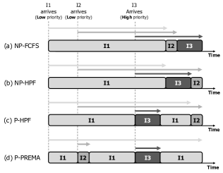
Figure 2: Timeline of three inference tasks (I1$-$I3) using (a) non-preemptive FCFS (NP-FCFS), (b) non-preemptive, high-priority first (NP-HPF), (c) preemptive, high-priority first (P-HPF), and (d) our preemptive and predictive PREMA schdeuler (P-PREMA).

Building upon our preemptible NPU, we propose our predictive multi-task scheduling algorithm (PREMA) that effectively balances latency, fairness, throughput, and SLA (service level agreement) satisfaction. A key challenge of a preemptive, high-priority first (Figure 2(c)) policy is that short-running low-priority tasks (I2) can be starved from scheduling and experience a relatively much severe performance slowdown. If we were to be able to estimate the job length of I2, a better scheduling decision would be to have I2 preempt I1, quickly finish its execution and have I1 resume execution as shown in Figure 2(d). This allows the average latency all tasks experience to be minimized while allowing the high-priority I3 to receive high-quality service. Interestingly, while knowing a given job’s remaining work a priori is very challenging, we make the unique observation that the computation and memory access behavior of a DNN algorithm as well as the NPU architecture that executes it are both highly deterministic and predictable. This allows us to develop a prediction model that reliably estimates the job size of each inference task (i.e., network-wide DNN execution time), which is utilized to meet latency demands while not sacrificing throughput or SLA. To summarize our key contributions:

• To the best of our knowledge, our work is the first to explore multi-tasked DNNs, an important and emerging problem space that has not been addressed by prior work.

• This paper is the first to provide an in-depth, quantitative analysis on the architectural support required for enabling preemption on NPUs.

• We propose PREMA, which utilizes preemption and the ability to estimate end-to-end DNN inference time to intelligently balance latency, throughput, and SLA satisfaction for multi-tasked DNNs.

II Background

II-A DNN Computation and Memory Accesses

Today’s most widely deployed DNNs can broadly be categorized as convolutional and recurrent neural networks (CNNs and RNNs). Both of these are designed by combining multiple layers, the most notable ones being the convolutional (CONV), activation (ACTV), pooling (POOL), fully-connected (FC), and recurrent layer (RECR). Inter-layer data dependencies are extracted at compile-time using the DNN topology and is encapsulated as a direct acyclic graph (DAG), each graph node representing a layer. For inference, a layer-wise computation is performed sequentially from the first layer to the last layer. Each layer applies a mathematical operation to the input activations (X) and stores the results as the output activations (Y). Certain layers such as CONV/FC/RECR have layer-specific weights (W), the values of which change during the training process, but are statically fixed for inference.

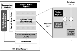
(a)

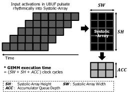
(b)

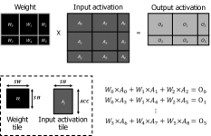
(c)

Figure 3: (a) Systolic-array based microarchitecture, (b) the weight-stationary dataflow that multiplies the incoming activations with the weights latched inside the PEs in fixed number of clock cycles, and (c) a tiled GEMM operation. Note that the outer-tiles located in the rightmost/bottommost edges of the weight matrix (W_2-5) and input activation matrix (A_2,5-8) can be smaller in size than the inner-tiles.

II-B Baseline NPU Architecture

Following the co-processor model as employed in today’s NPUs, our baseline NPU is attached to the I/O bus as a slave device (Figure 3). The set of operations to conduct for a given layer is compiled down into multiple CISC instructions, which are populated into the NPU instruction buffer by the CPU. The ISA we assume in our NPU is as follows:

• LOAD_TILE: loads input activations (weights) from DRAM to the unified activation (weight) buffer.

• GEMM_OP: performs a matrix-multiplication between the weight tile (SW$\times$SH) and input activation tile (SH$\times$ACC) using the GEMM unit, generating the output activation tile (SW$\times$ACC) that is stored into the accumulator queue.

• CONV_OP: convolution operation is first lowered into a matrix-multiplication operation [10, 11], and then the GEMM_OP operation is conducted to generate the output activation tile.

• VECTOR_OP: performs element-wise operations to the input using the vector unit, for instance, applying activation functions (e.g., ReLU, sigmoid, tanh) to the output activations generated by GEMM_OP, CONV_OP, or conducting vector additions.

• STORE_TILE: stores the output activations from the unified activation buffer to DRAM.

The NPU microarchitecture is based on Google TPU [4] as it executes both CNNs and RNNs (Figure 3(a)). The GEMM unit is based on systolic-arrays, containing $128\times 128$ Processing Elements (PEs), each of which performs a $16$-bit MAC operation per cycle. Each PE contains a weight register storing a single $16$-bit value. The weight registers are staged through a weight buffer directly from DRAM using the LOAD_TILE instruction during the weight load process. Input activations are stored inside the unified activation buffer (UBUF) using LOAD_TILE and are streamed into the GEMM unit for matrix-multiplication. The output activations computed by the GEMM unit via GEMM_OP or CONV_OP instructions are stored into the accumulator queue (ACCQ). The NPU architecture employs Google TPU’s weight-stationary dataflow [1] as shown in Figure 3(b): the values latched inside the PE weight registers remain stationary during the GEMM_OP execution and the input activations in the UBUF pulsate rhythmically through the GEMM unit, sequentially storing the output activations into ACCQ. Once GEMM unit’s operation is complete, the output activations can be stored back into the UBUF or can optionally be stationary inside ACCQ for another round of accumulation if the overall matrix-multiplication is tiled across multiple iterations of GEMM_OP. This is because the GEMM unit can only hold as much as 128$\times$128 weights at any given point, so for those layers having weights (and activations) larger than what can be buffered, the GEMM operation is tiled across multiple GEMM_OP/CONV_OP operations (Figure 3(c)). Intelligently overlapping DMA-invoked LOAD_TILE/STORE_TILE operations while the compute engine is busy executing GEMM_OP/CONV_OP instructions is key in efficient hardware utilization. Using the deterministic DNN dataflow, the baseline NPU utilizes task-level parallelism using double-buffering to concurrently utilize compute and memory resources.

II-C Research Scope

To optimize server compute density, cloud inference servers typically contain multiple GPUs/NPUs within a single node. Kubernetes [12] is a popular framework for managing system-node user requests and cloud ML inference systems. Per scheduling policy as implemented in Kubernetes, user requests are routed to each inference server. Requests queued inside each GPU/NPU is then handled by the runtime system like TensorRT Inference Server (i.e., our baseline NP-FCFS scheduler, see Figure 1). As this work is the first to explore multi-tasked DNNs, we focuse on how to best schedule user requests “after” Kubernetes routes incoming requests to each NPU. Exploration of efficient system-node level scheduling policy under a multi-NPU system (using our preemptible NPUs) will be interesting, but it is beyond the scope of this work and we leave it as future work.

II-D Related Work

GPUs employ a SIMT execution model and thread scheduling is managed in thread-block granularity, which previously studied GPU preemption solutions [13, 14] are primarily founded upon. As GPU’s SIMT programming abstraction, the underlying GPU microarchitecture, and task scheduling granularity significantly differs to how NPUs are programmed and executed (e.g., single-threaded, vector/matrix based execution), a direct, quantitative comparison between our NPU preemption architecture and prior GPU preemption solutions is challenging, if not impossible. Below we qualitatively summarize relevant prior studies. Preemptive CPU multi-tasking is traditionally supported using context switching, which has reasonable preemption latency and performance overheads [15]. Providing preemptive multi-tasking support in GPUs however is non-trivial as brute-force context switching can incur significant performance loss. This is because a significant fraction of on-chip SRAM is dedicated to preserving thread contexts such as register-files or scratchpads. Such massively sized execution context (which is in the orders of several tens of MBs) comes at a cost of high preemption latency, which can take several tens of $\mu$secs and cause severe performance loss. As such, prior GPU preemption studies have focused on alleviating the performance overheads of preemption, proposing various preemption mechanisms such as GPU core draining [13], flushing (re-execute for idempotent kernels) [14], compiler-optimizations that help reduce the size of the checkpointed context states (e.g., removing dead registers) [16], and various software optimizations [17, 18, 19]. There have been a series of pioneering work by Chen et al. [20, 21] that studies QoS issues for latency-sensitive DNN workloads assuming non-preemptive GPUs for inference, whereas our work focuses on ML acceleration using preemptible NPUs.

Aside from these closely related prior work, there has been a large body of studies exploring the design of architectures for ML [22, 23, 24, 25, 26, 27, 28, 29, 30, 31, 32, 33, 34, 35, 36, 37, 38, 39, 40, 41, 42] with recent interest on sparsity-optimized solutions for further energy-efficiency improvements [43, 2, 44, 45, 46, 47, 48, 49, 50, 3, 51, 52].

III Methodology

TABLE I: NPU configuration parameter.

Processor architecture
Systolic-array dimension	$128\times 128$
PE operating frequency	$700$ MHz
On-chip SRAM size (activations)	$8$ MB
On-chip SRAM size (weights)	$4$ MB
Memory subsystem
Number of memory channels	$8$
Memory bandwidth	$358$ GB/sec
Memory access latency	$100$ cycles

Simulation methodology. We developed a cycle-level performance model based on Google’s TPU as described in [4] and public patents from Google [53, 54, 55, 56] (Table I). The performance model has been cross-validated against both SCALE-Sim [57] and Google Cloud TPUv2 [58]. As DNN’s computation and memory access characteristic exhibit high data locality and a deterministic dataflow, system performance is less sensitive to the underlying behavior of the DRAM microarchitecture (e.g., row/bank conflicts). To reduce simulation time, we follow the methodology from prior work [3, 2, 45] where the memory subsystem is modeled as having fixed memory bandwidth and latency, rather than employing a cycle-level DRAM simulator [59, 60, 61].

Benchmarks. Constructing multi-tasked DNNs representative of real-world cloud inference is challenging for two reasons. First, existing ML benchmarks [62, 63] focus on a single DNN application. Second, the set of inference applications deployed at the cloud, the user request rate, and its priority levels are vendor-specific, proprietary information not publicly disclosed. We therefore take the following approach in constructing our workloads. Based on recent studies from several hyperscalars [64, 65], a total of eight DNN models considered representative of cloud inference are selected. Specifically, four CNN models with diverse convolution configurations (e.g., various filter dimension sizes, separable/depth-wise convolutions) have been chosen, namely AlexNet, GoogLeNet, VGGNet, and MobileNet (CNN-AN/GN/VN/MN [66, 67, 68, 69]). We also include four LSTM RNN models developed for cloud inference as follows. Two RNN topologies from MLPerf cloud inference suite [62], developed for sentiment analysis (RNN-SA) and machine translation are chosen. We instantiate two instances of the machine translation model (RNN-MT(1$-$2)), which is (randomly) chosen for usage as “English-to-(German/Korean/Chinese)” translation service (Figure 9). We also include one automatic speech recognition (RNN-ASR) application based on the well-known “Listen, Attend and Spell” model [70]. Using these eight DNNs, we construct multi-tasked DNN workloads based on the methodology suggested by prior GPU preemption studies [13, 14] as described below. First, we randomly select N inference tasks among the eight DNNs in order to construct a multi-tasked workload. We then assume uniform random distribution on when each task can be dispatched to the NPU. The dispatched task is randomly assigned with a priority level among low, medium, and high. Upon the arrival of a given task to the NPU scheduler, the preemption mechanism (Section IV-D) and preemption policy (Section V-C) chosen dictate the dynamics of whether any one of the schedulable task can preempt the executing task or not (i.e., depending on the execution context, any given task can be preempted more than once or not at all). The following sections further detail our methodology as necessary (e.g., the number of co-scheduled tasks (N) chosen per each workload, batch size, number of time-unrolled sequence length for each RNN, $\ldots$).

Metrics. We use the metrics as suggested by Eyerman et al. [71] (Equation $1$$-$$2$). Concretely, we derive normalized turnaround time (NTT) of each task, its arithmetic average across all multi-tasked workloads (Average NTT, ANNT), system throughput (STP), and fairness. NTT is a measure of a task’s performance slowdown when executing with other tasks ($C_{i}^{multi}$), compared to its isolated execution ($C_{i}^{single}$). Rather than single-handedly measuring how much useful work was done, STP as defined in [71] considers each task’s performance slowdown under a multi-programmed execution, so optimizing STP requires maximizing per-program progress when co-executing multiple programs. Fairness is a measurement of equal progress of tasks under a multi-tasked context, relative to their isolated execution.

$$ANTT=\frac{1}{n}\sum_{i=1}^{n}\frac{C_{i}^{multi}}{C_{i}^{single}},\hskip 10.00002ptSTP=\sum_{i=1}^{n}\frac{C_{i}^{single}}{C_{i}^{multi}}$$ (1)

$$Fairness=\min_{i,j}\frac{PP_{i}}{PP_{j}},\hskip 10.00002ptPP_{i}=\frac{(\frac{C_{i}^{single}}{C_{i}^{multi}})}{(\frac{Priority_{i}}{\sum_{j=1}^{n}Priority_{j}})}$$ (2)

IV Designing A Preemptible NPU Architecture

This section details our first key contribution, which is the development of several generic preemption mechanisms tailored for the architectural characteristics of NPUs.

IV-A Preemption Architecture

A preemptible NPU should track the context of the multiple DNN tasks inside the job scheduler. We extend the NPU to include a preemption module (Figure 3(a)) that uses the inference task context table to track each task’s ID (TaskID), task priority, and any other state that is utilized by our scheduling framework (Figure 4). The task queue inside the preemption module receives new inference service requests by the CPU. Depending on the chosen preemption mechanism and scheduling policy, the preemption module takes the necessary action to meet target scheduling objectives such as latency, fairness, and throughput. As the scope of this work is on temporal multi-tasking, the multiple inference tasks do not spatially share the NPU substrate concurrently. Accordingly, the on-chip memory hierarchy need not have to distinguish between different tasks and the preemption handler routine can safely checkpoint or flush the preempted task’s on-chip context state (the size of which is governed by the chosen DNN dataflow and preemption mechanism, detailed in following sections) to memory as appropriate. Note that the multiple inference tasks inside the NPU job scheduler do share memory. The MMU therefore utilizes each task’s TaskID, which functions as an ASID, to check for protection violations for reads and writes to memory.

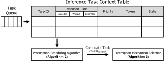
Figure 4: PREMA inference task context table. Detailed usage of each entry field in our scheduler is discussed in Section V-C.

IV-B Checkpointing Requirements

A key requirement for preemption is to determine what is the distinct context state that the NPU must preserve to resume execution in the future. For inference, the weight values (W) do not change, so any on-chip space dedicated for storing weights need not be checkpointed. In terms of activations, the CONV/FC/RECR layers conduct an out-of-place operation so the on-chip storage for input activations (X) and output activations (Y) are distinctively separated (i.e., two separate mallocs for X and Y). The ACTV and POOL layers, on the other hand, are designed as an in-place operation to save memory space, where the output activation values are derived on-the-fly and stored back into the original storage space allocated for input activations (i.e., X and Y are identical). Note that ACTV/POOL layers can be fused with the preceding CONV/FC/RECR layers through a VECTOR_OP operation using the vector unit to save memory bandwidth consumption and latency for fast inference [72]. Consequently, upon a preemption request, the context state that is checkpointed is the newly derived output activations potentially stored inside the UBUF and ACCQ. Overall, the major checkpointing overhead comes from the output activations that have been derived up to the point the preemption request is to be serviced. Below, we discuss three preemption mechanisms that trade-off checkpointed state size, preemption latency, fairness, and system throughput.

IV-C Preemption Mechanisms for NPUs

The basic principle of preemption in OS is to first checkpoint the execution contexts of the preempted process to memory and then context switch to the preempting process. The first preemption mechanism we explore follows this basic preemption technique (called CHECKPOINT) and checkpoints the context of the preempted task to memory. The preempted context preservation, restoration, and context switching to the preempting inference task is implemented with a software trap routine. Because a single matrix-multiplication operation between an input activation tile (streamed in from the UBUF) and the weight tile (latched inside the GEMM unit) is conducted via a single GEMM_OP instruction under our CISC ISA, the preemption trap routine under CHECKPOINT is called upon after the currently issued GEMM_OP instruction is completely executed and committed the output activation values into the ACCQ. Accordingly, the execution context that is checkpointed is the output activations temporarily stored inside the UBUF and the ACCQ. The trap routine uses the DMA unit to maximally utilize memory bandwidth for storing the context state back to main memory, similar to how STORE_TILE operations are executed.

To alleviate the preemption latency overhead of CHECKPOINT, our second preemption mechanism termed KILL is aimed at providing the fastest user-responsiveness by immediately terminating the current task’s execution without checkpointing the execution context. While an obvious limitation of KILL is that it can harm system throughput (i.e., the computations done up to the preemption point are wasted as execution must restart from scratch), it is possible for KILL to present a good tradeoff point than CHECKPOINT if KILL is invoked during the early phases of an inference execution. The last preemption mechanism we explore is DRAIN, a design point located at the other end of the spectrum of KILL. Using DRAIN, the preempting task cannot get scheduled until the current inference task completely finishes the remaining network-wide computations. Strictly speaking, DRAIN does not preempt the current task’s execution and arguably should not be categorized under a preemption mechanism. However, as detailed in Section V, our PREMA scheduler leverages DRAIN as a powerful tool for intelligently coordinating job scheduling in multi-tasked inference. We therefore study DRAIN as part of our preemption mechanisms.

(a)

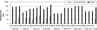
(b)

Figure 5: (a) Preemption latency (i.e., time to checkpoint the execution context) for each preemption mechanism, and (b) the preempting task’s wait time from when it was first requested until it gets serviced. The reported result (y-axis) is averaged across multiple experiments where the preempting, high-priority task and its batch size are both chosen randomly among the eight DNNs (Section III) and three possible batch size ($1$/$4$/$16$). As the checkpointed state size (and accordingly the preemption latency and wait time) is a function of both the preempted task and its batch size, we separately plot the evaluted metrics depending on these two parameters in the x-axis.

IV-D Effect of the Preemption Mechanisms

To evaluate the effectiveness of our three preemption mechanisms while isolating the effect of the scheduling policy that utilizes them, we use two simple scheduling policies as discussed in Figure 2: the baseline, non-preemptive first-come first-serve scheduler (NP-FCFS) and a preemptive, high-priority first scheduler (P-HPF). A multi-tasked workload containing two DNN inference tasks is constructed where the low-priority task is first executed but is later preempted by a high-priority task using P-HPF. We assume uniform random distribution on the possible preemption point across the low-priority task’s execution time. Figure 5 shows the effect of our preemption mechanisms on preemption latency and the preempting task’s waiting time before it gets serviced. Note that DRAIN serves as a baseline comparison point for our studied mechanisms as it is not able to preempt a running task’s execution, having zero preemption latency with a long wait time for the preempting task. Following the intuitions as discussed in Section IV-C, KILL incurs no preemption latency whereas CHECKPOINT suffers from a sizeable preemption overhead, leading to an average $12$ $\mu$sec additional latency. The effect of these preemption mechanisms on STP and the preempting task’s NTT improvement however is rather surprising (Figure 6). KILL achieves the highest improvements in NTT as the preempting task can be serviced immediately under P-HPF. KILL however suffers from a larger STP degradation than CHECKPOINT. Despite such differences in preemption overheads between KILL and CHECKPOINT, its effect on NTT is marginal, showing an average $3.08\times$ and $3.06\times$ NTT improvement for KILL and CHECKPOINT, respectively. Such (rather counter-intuitive) result is due to the recent trends in ML algorithms where state-of-the-art DNNs contain tens to hundreds of layers across the network. Across the benchmarks we study, the preemption latency is usually in the orders of $\mu$secs (worst case latency being $59$ $\mu$sec when the entire $8$ MB of UBUF/ACCQ is checkpointed) and accounts for less than $2.6\%$ of the overall execution time (i.e., network-wide inference time is usually in the orders of several msecs, $0.5$ to $45$ msecs among the eight DNNs we considered in this study, Section III). Consequently, our analysis shows the key observation that the effect of preemption mechanisms on preemption latency is practically negligible for NPUs as the overhead is amortized over the (relatively) long inference time. That being said, preemption mechanisms do have a significant impact on system throughput and the preempting task’s waiting time. For instance, while KILL and CHECKPOINT cause zero to negligible waiting time relative to the network-wide inference time, the waiting time of DRAIN is sensitive to when the preemption request is made (e.g., close to zero wait time if preemption request is made near the end of network’s execution), showing an average $5.3$ msec of wait time.

(a)

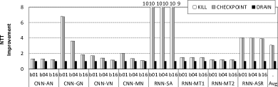
(b)

Figure 6: (a) System throughput and (b) the preempting task’s NTT improvement, normalized to NP-FCFS. Methodology follows that of Figure 5 but we now plot STP and NTT as a function of what the preempting task and its batch size was on the x-axis. This is because the overall execution time of the preempting task plays a key role on the dynamics of STP and NTT. For instance, CNN-GN and RNN-SA is relatively short-running, so it is beneficial in terms of STP (Equation 1) to have these workloads preempt the current task and quickly finish execution via KILL/CHECKPOINT. We detail how PREMA utilize such behavior in Section V (Algorithm 3).

IV-E NPUs: To Preempt or Not To Preempt?

Overall, we observe that preemption latency (i.e., checkpointing overhead of preemption) itself only causes secondary effects on the preempted/preempting task because of the long-running nature of DNN inference nowadays. The choice of preemption mechanism does however dramatically impact the preempting task’s waiting time and system throughput, so the job scheduler must consider its implication in making scheduling decisions. As we quantitatively demonstrate in Section VI-E, CHECKPOINT shows superior performance and robustness than KILL on all our evaluations because CHECKPOINT provides comparable latency guarantees of KILL while achieving much higher STP. For brevity and clarity of explanation, the next section assumes CHECKPOINT as the primary NPU preemption mechanism for our PREMA scheduler. We re-visit the sensitivity of our proposal on the selection of preemption mechanism (i.e., CHECKPOINT vs. KILL) in Section VI-E.

V PREMA: A Predictive Multi-Task Scheduler

This section details the next key contribution of our study: a predictive multi-tasked DNN scheduling algorithm (PREMA) for preemptible NPU architectures.

V-A Key Challenges and Proposed Approach

One key limitation of a preemptive, high-priority first scheduler (P-HPF) is that short-running low-priority tasks can be starved from scheduling and suffer from severe performance penalties. For scenarios as illustrated in Figure 2(c), a better scheduling decision would be to allow the low-priority, but short-running I2 to preempt the execution of I1 and quickly finish its execution and resume I1’s execution afterwords (Figure 2(d)). While this lengthens the latency of I1, the relative performance slowdown I1 receives is much smaller when compared against the slowdown I2 would have experienced had I2 not preempted I1 (Figure 2(c)). In practical scenarios however, the remaining size of any given job (i.e., job length) is not known a priori so developing a scheduler that intelligently utilizes preemption as described above becomes challenging. We propose PREMA, a “preemptive” and “predictive” NPU scheduler that considers both the task size and its priority level to balance latency, throughput, and SLA satisfaction. A prediction model that estimates the network-wide DNN latency for each task is proposed, which is utilized by PREMA to meet target scheduling objectives. A DNN is expressed as a DAG where each graph node corresponds to a DNN layer. Accurately estimating the end-to-end, network-wide DNN latency requires methods to predict 1) the node-level execution time but more importantly 2) how many nodes are executed overall during the course of inference. We detail our prediction algorithm below.

V-B PREMA Prediction Model

Our predictor consists of two components: 1) node-level execution time estimation (i.e., predicting the latency incurred per each DNN layer), and 2) predicting how many nodes are executed overall to infer end-to-end network-wide latency. To the best of our knowledge, this work is the first to suggest a practical solution in estimating the input-dependent, dynamically determined seq2seq style DNN sequence length in a static manner.

Node-level Latency Prediction. We make the key observation that the behavior of both the target algorithm and the architecture that executes it are highly regular and deterministic. As discussed in Section II-A, any given layer’s configuration is constructed at compile time and the DNN weight values are statically fixed upon deployment. As the layer computation and its memory access behavior are highly deterministic, an effective way to predict node-level latency is to profile the average latency of a target DNN layer and bookkeep it to utilize later for network-wide latency prediction. We empirically validate such key observation through a thorough characterization study on both NPUs and GPUs as detailed below:

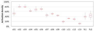
Figure 7: Changes in VGGNet’s per-layer activation density during $1000$ inference tests in ImageNet. Similar observations were made for AlexNet/GoogleNet but we omit the results due to space constraints.

1. We profiled four off-the-shelf GPUs ([73, 74, 9, 75]) executing $50$ different layer types and configurations (Section II-A) using cuDNN/cuBLAS [76, 77]. For a given layer configuration, the measured latency across $1000$ inference tests always fall within $4\%$ of the average. This is expected as these GPU kernels are not input data-dependent, exhibiting no to little branch or memory divergence [78].

2. Similar observations were made for Google Cloud TPUv2 when profiling the latency of $100$ different layer configurations, showing an average $0.2\%$ standard deviation in terms of execution time.

3. We also profiled the inference time over sparsity optimized NPUs by implementing a cycle-level performance model of the state-of-the-art SCNN design [3]. When profiled across $500$ ImageNet images using pruned version of CNN-AN/GN/VN, the execution time never deviated more than $14\%$ (average $6\%$) of the average latency. The reason behind its predictable execution time is twofold: (1) weight sparsity is fixed once pruned and retrained for deployment, so weight sparsity itself causes no variation in latency, (2) activation sparsity, which is input data-dependent, was shown to exhibit small per-layer variation at inference time (Figure 7).

Given such high determinism, our initial proposal is to profile the average per-layer latency of a target DNN and utilize it for predicting the network-wide inference time – an approach applicable for both GPUs and NPUs. Our study however is based on a simulated version of TPU, so utilizing the profiled measurements of the (blackbox) Google Cloud TPUv2 as-is for predicting per-layer latency is less meaningful under our evaluation setting. Interestingly, another unique observation we make is that state-of-the-art NPUs [29, 23, 24, 4, 79, 80] commonly leverage the deterministic dataflow to manually orchestrate computations with memory accesses to maximally utilize compute and memory resources. A common design practice in NPUs [29, 22, 23, 2, 3] is to utilize this deterministic dataflow to leverage task-level parallelism to overlap the compute phase and memory phase for maximum efficiency. Naturally, the underlying NPU microarchitecture causes differences in how computation itself will be carried out (e.g., systolic-array based vs. spatial architectures). Consequently, as an alternative to the profile-based node-level predictor, we propose an architecture-aware analytical model that estimates the NPU’s node-level execution latency using the deterministic dataflow. As a proof-of-concept, we describe the inference time prediction model tailored for our baseline systolic-array NPU architecture below (Algorithm 1).

Algorithm 1 Inference Time Prediction Model

1:$Time_{estimated}=0$

2:for $\textbf{each}\ (m,k,n)\ \textbf{in}\ Layers$ do

3:    $C_{1}=ACC+SH+2\times SW$

4:    $M_{1}=(SH\times SW+SH\times ACC)/{BW_{DRAM}}$

5:    $Time_{innertile}=\max(C_{1},\ M_{1})$

6:    $C_{2}=(n-\lfloor{\frac{n}{ACC}}\rfloor\times ACC)+SH+2\times SW$

7:    $M_{2}=(SH\times SW+SH\times(n-\lfloor{\frac{n}{ACC}}\rfloor\times ACC))/BW_{DRAM}$

8:    $Time_{outertile}=\max(C_{2},\ M_{2})$

9:    $\phi=if(n-\lfloor{\frac{n}{ACC}}\rfloor\times ACC=0)\ then\ 0\ else\ 1$

10:    $Time_{estimated}\ \mathrel{+}=$

11:$\qquad\qquad(\lfloor\frac{m}{SW}\rfloor\times\lfloor\frac{k}{SH}\rfloor\times\lfloor\frac{n}{ACC}\rfloor\times Time_{innertile}\$

12:$\qquad\qquad+(\lfloor\frac{m}{SW}\rfloor\times\lfloor\frac{k}{SH}\rfloor\times\phi)\times Time_{outertile})\$

13:end for

14:return $Time_{estimated}$

Case Study: Prediction Model for Systolic-Arrays. A GEMM_OP between a (m$\times$k) weight and a (k$\times$n) input activation is first tiled to be compatible with the systolic-array microarchitecture as illustrated in Figure 3(c). The (SH$\times$ACC) input activation tile is streamed into the GEMM unit in a rhythmic fashion and is multiplied with the (SH$\times$SW) weight tile, which stores the (SW$\times$ACC) output activation tile inside ACCQ in fixed number of clock cycles as summarized in Figure 3(b). Because the compute phase of the current GEMM_OP (C₁, line 3) is overlapped with the memory phase spent in fetching the two input tile matrices for the next GEMM_OP (M₁, where BW_DRAM refers to the off-chip memory bandwidth, line 4), the time spent in any given inner-tile’s GEMM_OP can be estimated as shown in the pseudo-code in line 5 (Figure 3(c) describes inner vs. outer tiles). The prediction model similarly takes into account the compute and memory phases spent in handling the outer-tiles around the edges (line 6$-$9). By accounting for the total number of inner/outer-tiles within a given layer, the prediction model is able to estimate the (node-level) layer-wise execution time (line 10). We next discuss our practical prediction mechanism for estimating the total number of nodes to execute in the DAG (i.e., number of layers in line $2$), enabling a network-wide execution time prediction (line 12).

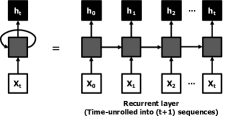
(a)

(b)

(c)

Figure 8: (a) Recurrent layer time-unrolled into variable sequence length, and RNN applications with (b) linear and (c) non-linear relationship between input and time-unrolled output sequence lengths.

(a) Translation (English-German)

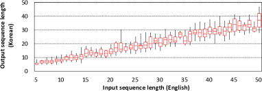
(b) Translation (English-Korean)

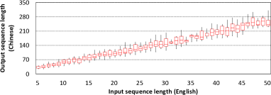
(c) Translation (English-Chinese)

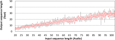
(d) Automatic speech recognition

Figure 9: Profile-driven characterization graph for non-linear RNNs. The total number of time-unrolled recurrence length (y-axis) is shown as a function of the length of the input sequence (x-axis). (a-c) We used Google Translate [81] and WMT-2016 Evaluation Campaign Training data [82] test set to translate 1500 English sentences into target languages. (d) Python Google Speech Recognition API [83] and the LibriSpeech ASR corpus [84] were used to profile 1500 speech recognition data. We omit the characterization graph for linear RNNs (e.g., sentiment analysis, language models) for brevity as the output sequence length of these applications are statically determined by the input sequence length.

Predicting Total Number of Executed Nodes in DNNs. CNNs have a static DAG structure so the total number of nodes to execute is statically known (line $2$ in Algorithm 1). RNNs however have variable number of graph nodes to traverse within the DAG because the size of time-unrolled recurrence length (a.k.a output sequence length) is input data-dependent, rendering a static estimation of RNN’s network-wide latency challenging (Figure 8(a)). Nonetheless, the unrolled recurrence length is, by design, correlated with the input sequences because RNNs are trained to extract temporal relationship across input sequences and utilize it for generating output sequences. Also, while RNNs can receive any variable length input sequence, the length of the input sequence itself is statically known before inference takes place, a property of which is utilized by several GPU backend libraries to increase parallelism and thread occupancy [76]. Consider the RNN-based sentiment analysis application [85, 86, 87] in Figure 8(b). Here we know beforehand that the input sequence length is $5$ (including the end-of-sequence (EOS) token), before the RNN is executed for inference. Additionally, note that the total number of recurrence unrolled is identical to the number of input sequence as the final RNN output gets generated as a softmax vector right after the $5$ unrolled recurrent layers are executed. Similar usage of RNNs that exhibit a static, linear relationship between the input and output sequence length include language models [88, 89] and many others. Predicting the time-unrolled recurrence length for these RNN applications is trivial as it is statically determined by the input sequence length. There are however applications such as machine translation [90, 91] or speech recognition [92, 93] exhibiting a dynamic, non-linear relationship between the input and output sequence lengths. These applications are commonly implemented using the sequence-to-sequence (seq2seq) DNN architectures where a variable-length input sequence is mapped to a variable-length output sequence [94]. Consider the RNN model in Figure 8(c) which translates an English sentence into German. The translated output words start getting generated after a sequence of input words are fed into the encoder-decoder architecture, terminating the translation process once the decoder outputs the EOS token. While this example illustrates a simple, one-to-one translation of each English word into German, the number of translated output words is a function of the target language’s vocabulary, grammer, translation context, and others (e.g., translation of the same $4$-word English sentence into Korean/Chinese/Spanish results in a $3$/$7$/$4$-word output sentence, respectively). Nevertheless, what holds true even for these non-linear RNN applications is that the output sentence length is highly correlated with the size of the input sentence length. Figure 9 shows our chracterization study where the time-unrolled recurrence length (y-axis) is depicted as a function of the number of input sequence length (x-axis). While some outliers do exists (represented by the minimum-maximum range in this boxplot figure), the 25$-$75$\%$ interquartile range consistently falls within a narrow boundary. Across a wide range of applications, we observe two unique characteristics of RNN inference:

1. The time-unrolled recurrence length is a function of how the model has been trained so the number of unrolled sequence at inference time will likely fall within the profiled set of output sequence lengths.

2. The profiling overhead to construct the RNN characterization graph is paid once per each model and is amortized over all future inferences to this model (e.g., NVIDIA V100 has an inference throughput of $70,002$ RNN input samples per second when tested for OpenNMT [91], meaning it is able to test one million inputs within $15$ seconds [95]).

Based on such key observations, we propose to construct the characterization graph as exhibited in Figure 9 using the inference test results across the training and/or validation dataset. Such profile-driven characterization graph is effectively a regression model that predicts the time-unrolled output sequence length. As such, we propose to build this regression model as a software-level lookup table, which is indexed by the number of input sequence length (x-axis in Figure 9, a value that is statically known before inference begins) and returns the geometric mean value of the profiled recurrence length across the inference test dataset.

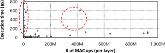
Figure 10: Each data point represents a given layer’s total number of MAC operations required (x-axis) and the resulting execution time (y-axis). All the layers that are part of our $8$ benchmarks are considered and are sorted in the x-axis based on the number of MAC operations per each layer. The data points inside the red circled region are layers that underutilizes the systolic-array’s math operators (e.g., $1\times 1$ CONV layers from MobileNet/GoogLeNet), suffering from low effective throughput and long execution time.

Putting Everything Together. As the parameters used to calculate the network-wide Time_estimated are either known a priori or estimated using our profile-driven regression model, the CPU can derive this value before sending it as part of the context state when requesting inference to the NPU. We expect the latency of deriving Time_estimated in software will be negligible, but if necessary a lightweight FSM logic that implements Algorithm 1 can be synthesized in hardware. Note that blindly using the absolute number of MAC operations conducted per DNN as a proxy for estimating an inference task’s execution time will lead to misleading results as it does not consider how the application is actually mapped into the underlying NPU architecture. As shown in Figure 10, the actual execution time of any given layer is not necessarily proportional to the total number of MAC operations that are part of a layer’s execution, underscoring the importance of an architecture-aware prediction model.

V-C “Token”-based Scheduling Framework

Building upon the preemption mechanism (Section IV) and predictor model (Section V-B), we now present our token-based PREMA scheduling framework. The PREMA scheduler consists of the following two-step procedure: (1) the scheduling policy (Algorithm 2) determines which candidate inference task to execute next (which can potentially preempt the currently executing task), and (2) once the candidate task is chosen, a preemption mechanism (Algorithm 3) is selected that is most appropriate for the current execution context (Figure 4). The aformentioned two-step procedure is undertaken whenever PREMA scheduler wakes up under the following three conditions: (1) a new task is dispatched to the NPU, (2) an already executing task finishes execution, or (3) a pre-determined scheduling period time-quota (line $5$ in Algorithm 2) has elapsed.

Algorithm 2 PREMA Scheduling Algorithm

1:Initialization

2:for $\textbf{each}\ Task_{i}\ \textbf{in}\ ReadyQueue$ do

3:    $Token_{i}\leftarrow UserDefinedPriority_{i}$

4:end for

5:Each scheduling period

6:for $\textbf{each}\ Task_{i}\ \textbf{in}\ ReadyQueue$ do

7:    $Token_{i}+=UserDefinedPriority_{i}\times Slowdown_{normalized}$

8:end for

9:$Candidates=[Task_{i}\ \textbf{if}\ Token_{i}\ >\ Threshold]$

10:$TaskID_{candidate}\leftarrow FindShortestEstimatedJob(Candidates)$

11:return $TaskID_{candidate}$

PREMA scheduling policy. Under PREMA, each task is assigned with tokens which determine its opportunity to get picked up by the scheduler for execution. Algorithm 2 provides a pseudo-code of our PREMA algorithm. Whenever a new task is dispatched from CPU to NPU, the task is assigned with a fixed, user-defined priority level (UserDefinedPriority) and PREMA grants an initial number of tokens per its priority level, which is statically pre-determined as a configuration parameter (line $3$, Table II). Among all the tasks that have been dispatched to the scheduler (ReadyQueue in line $6$), the scheduler selects a group of candidate tasks (Candidates) that are in urgent need for scheduling. A task can be selected as part of the candidate group when the number of tokens it possess is above a certain threshold (line $9$): this threshold value is dynamically determined by the task within the ReadyQueue that accumulated the largest number of tokens, where its number of tokens is rounded down (not up) to the closest UserDefinedPriority token value (i.e., $1$, $3$, or $9$). For instance, when the largest token value any given task possessed within all tasks inside the ReadyQueue is $8$, the threshold is set as $3$ not $9$ (i.e., if threshold is $9$, no single tasks can be categorized under Candidates for this given example). Our key novelty and innovation is the ability to dynamically adjust the number of tokens (not each task’s priority itself), using the task length prediction model as detailed in Section V-B, so that tasks with low priority can still receive scheduling opportunities. Specifically, PREMA implements the following token assignment (line $7$) and final candidate selection algorithm (line $10$) as means to balance latency, fairness, and SLA goals.

TABLE II: PREMA scheduler configuration.

Scheduling period time-quota	$0.25$ ms
Tokens assigned per UserDefinedPriority	$1/3/9$ (low/medium/high)

1. PREMA periodically assigns additional tokens to each tasks, proportional to the performance slowdown each task experienced ($Slowdown_{normalized}$) and its priority level (line $7$). $Slowdown_{normalized}$ is derived by comparing the amount of time it was left idle inside the ReadyQueue against its $Time_{isolated}$, which refers to a DNN task’s uninterrupted, isolated execution time. Because short-running tasks will experience a larger $Slowdown_{normalized}$ than longer ones, it will proportionally be assigned with more tokens within a given timeframe. This allows even low priority tasks to gradually accumulate more tokens and get more chances to be part of the Candidates group for execution.

2. Among the Candidates group, PREMA selects the final candidate that is estimated to be the “shortest” length job to optimize average latency (line $10$). Compared to blindly choosing the shortest job among all the tasks inside ReadyQueue, our token-based, priority-aware PREMA policy effectively services high-priority jobs’ latency requirements while also guaranteeing scheduling opportunities for short-running, low priority jobs.

3. It is worth pointing out that, without our task length prediction model (Section V-B), neither the dynamic token assignment policy (line $7$) nor the latency-optimal candidate selection algorithm (line $10$) can be implemented. Our PREMA provides an innovative way of utilizing the predictor to balance latency, fairness, and SLA goals.

Preemption mechanism selection. Once the next candidate task is chosen, our scheduling framework decides which preemption mechanism (between DRAIN and CHECKPOINT) is more advantageous for the current execution context (Algorithm 3). In certain cases, our dynamic mechanism selection algorithm chooses to override the scheduling policy’s recommendation (which is to preempt the running task and schedule Task_candidate) and let the currently running task complete execution uninterrupted via DRAIN (line $6$). At first glance, such decision appears to be counter-intuitive to the conclusions from Section IV-E as DRAIN could significantly lengthen the preempting task’s wait time. However, if the currently running task is nearing the end of execution (line $1$) and the preempting task still has a relatively long execution time (line $2$), it would be more productive to first finish execution of the current task to optimize ANNT (line $5$$-$$6$). Our prediction model is able to detect such scenario by comparing a task’s Time_estimated with how much it has actually executed so far (Time_executed). The dynamic preemption mechanism selection process is designed to leverage the prediction model to detect such scenarios and try to improve average latency as summarized in Algorithm 3.

Algorithm 3 Dynamic Preemption Mechanism Selection

1:$Task_{current}.Time_{remaining}\leftarrow$

2:$\qquad Task_{current}.Time_{estimated}-Task_{current}.Time_{executed}$

3:$Task_{candidate}.Time_{remaining}\leftarrow$

4:$\qquad Task_{candidate}.Time_{estimated}-Task_{candidate}.Time_{executed}$

5:$Degradation_{current}\leftarrow$

6:$\qquad Task_{candidate}.Time_{remaining}/Task_{current}.Time_{estimated}$

7:$Degradation_{candidate}\leftarrow$

8:$\qquad Task_{current}.Time_{remaining}/Task_{candidate}.Time_{estimated}$

9:if $Degradation_{current}>Degradation_{candidate}$ then

10:    return $Drain$

11:else

12:    return $Checkpoint$

13:end if

VI Evaluation

Multi-tasked workloads containing $8$ DNNs are constructed as discussed in Section III. To model the dynamic execution length of RNNs (Figure 8), we set the actual and predicted time-unrolled recurrent length as follows. For a target RNN, the input sequence length is randomly chosen among the profiled/tested set of input sentence lengths which were used to derive the PREMA regression model. The actual time-unrolled length of a given RNN is then randomly selected among all possible output sequence lengths as observed for that (chosen) input sequence length while constructing the profile-driven regression model (i.e., Figure 9). In this section, we report the averaged results across $25$ simulation runs of these multi-tasked DNN workloads per each policy.

VI-A Prediction Model Effectiveness

To quantify the usefulness of our prediction model while isolating the effect of preemption itself, we evaluate several scheduling policies on top of a non-preemptive multi-task scheduler (Figure 11). We first establish three scheduling policies that do not use our prediction model, namely 1) baseline first-come first-serve (FCFS), 2) round-robin among the multiple DNN models (RRB), and 3) high-priority first (HPF). We then include the three schedulers that use our prediction model, 1) a token-based scheduler (TOKEN) as discussed in Section V-C but schedules among the candidate groups in naive FCFS, 2) simply sorting the jobs based on task length and do shortest-estimated-job-first scheduling (SJF), and 3) our PREMA that combines the benefits of TOKEN and SJF. While HPF and TOKEN’s priority-awareness can help improve fairness than the naive FCFS and RRB, the non-preemptive scheduling algorithm and its inability to effectively utilize job length renders them suboptimal in terms of ANTT and fairness. Scheduling jobs that can complete the soonest is well-known to be optimal for average latency, so SJF achieves the highest ANTT. PREMA successfully balances ANTT, fairness, and STP, reaching $92\%$ of the ANTT of the latency-optimal SJF while maintaining fairness and its priority-awareness. The reason behind SJF and PREMA’s superior performance is clear: our prediction model effectively estimates the length of co-scheduled tasks (showing only $1.6\%$ estimation error) and helps reduce the wait time of short jobs, improving ANTT and fairness.

(a)

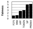
(b)

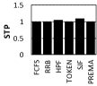
(c)

Figure 11: Improvements in (a) ANTT, (b) fairness, and (c) STP using the six schedulers over a non-preemptive NPU. TOKEN, SJF, and PREMA uses our predictor to estimate a task’s length.

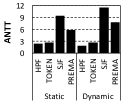
(a)

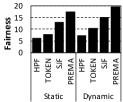
(b)

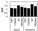
(c)

Figure 12: Effect of (static vs. dynamic) preemption mechanism on (a) ANTT, (b) fairness, and (c) STP on top of a preemptive scheduler. Preemption mechanism is statically fixed to CHECKPOINT (Section IV-C) for all static configurations whereas dynamic uses Algorithm 3 to adaptively choose between CHECKPOINT and DRAIN. All results are normalized to NP-FCFS.

VI-B Benefits of PREMA “and” Preemption

Figure 12 shows the benefits of our dynamic preemption mechanism (Algorithm 3) on top of the four preemption-enabled scheduling policies in Figure 11, when compared against statically choosing to always preempt via CHECKPOINT. Overall, our dynamic preemption mechanism provides superb ANTT, fairness, and STP for all scenarios. In particular, our PREMA coupled with dynamic preemption effectively balances ANTT, fairness, and STP, achieving $7.8\times$, $19.6\times$, $1.4\times$ improvement, respectively. The robustness of PREMA comes from its ability to adaptively and intelligently choose both the preemption mechanism and the scheduling policy that is most appropriate for the execution context. It is worth pointing out that the results in Figure 12 are averaged across all inference tasks without differentiating the priorities assigned to them, so the priority-aware PREMA provides much higher improvements for high-priority tasks, as opposed to the priority-unaware SJF which significantly degrades QoS for high-priority inference. We discuss PREMA’s efficiency on QoS below.

VI-C Quality-of-Service (QoS)

Service Level Agreement (SLA). Vendor-specific SLA targets are unique to each workload’s characteristics and are proprietary information not publicly disclosed. We therefore define the SLA target of our system as ($Time_{isolated}$$\times$N), where $Time_{isolated}$ refers to a DNN task’s uninterrupted, isolated execution time. By sweeping the value of N from $2$ to $20$ (i.e., SLA target with N equal or less than $1$ is practically an impossible QoS goal), we measure the fraction of SLA violated tasks for “all” inference requests as a function of the chosen preemption policy. As summarized in Figure 13, our PREMA significantly reduces the SLA violated rate below $10\%$ beyond an SLA target of N=4, a significant improvement over the $36\%$ SLA violation under NP-FCFS. Although SJF does better than PREMA in terms of SLA violation for all tasks, SJF significantly worsens the tail latency of high-priority requests as discussed below.

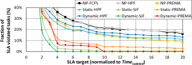
Figure 13: SLA violation rate for all tasks as a function of SLA target (x-axis, normalized to $Time_{isolated}$) and the scheduling policy. As SLA targets are set loose (from left to right in the x-axis), the violation rate monotonically decreases for all policies.

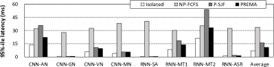
Figure 14: $95\%$-ile tail latency of high-priority inference tasks, assuming a single batch size.

Tail latency. Figure 14 shows the tail latency of high-priority inference tasks. Compared to when each task is executed in isolation, NP-FCFS significantly worsens tail latency by up to $85\times$ (average $21\times$). Preemptive SJF does better than NP-FCFS but still incurs up to $2.6\times$ higher tail latency. PREMA only incurs an average $40\%$ tail latency overhead (no more than $60\%$) compared to an isolated execution environment.

VI-D PREMA Prediction Accuracy vs. Oracle

We developed an oracular PREMA which utilizes each DNN’s exact execution time for scheduling. The predicted latency achieved over an average $98\%$ correlation with the simulated inference time, reaching $99\%$/$99\%$/$99\%$ of the STP/ANTT/SLA of oracle. Our prediction model shows competitive accuracy even compared to oracle because the ability to estimate relative latency differences (rather than absolute differences) robustly is key for PREMA scheduling objectives.

VI-E Sensitivity Study

Figure 15 shows the sensitivity of CHECKPOINT vs. KILL on the effect of (static vs. dynamic) preemption mechanisms. While KILL does improve ANTT and fairness in some cases (especially when combined with PREMA), KILL almost always performs poorly than CHECKPOINT. This is expected, as KILL does not show noticeable benefits than CHECKPOINT for ANTT while harming STP. Overall, CHECKPOINT achieve $87\%$/$24\%$/$77\%$ improvement in average ANTT/STP/fairness compared to KILL. Having the NPU be specialized to a single type of inference (e.g., CNN/RNN inferences are not mixed on a single server) also does not impact our proposal’s effectiveness. We also examined the sensitivity of PREMA on: 1) different batch sizes, 2) different preemption points (e.g., earlier/latter layers), and 3) different PREMA scheduler configuration (Table II). The effectiveness of PREMA generally remained intact, providing a minimum of $6.7\times$, $6.2\times$, and $1.4\times$ improvement in ANTT/fairness/STP for all sensitivity studies.

(a)

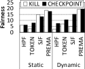
(b)

(c)

Figure 15: PREMA sensitivity to “CHECKPOINT vs. KILL”.

VI-F Implementation Overhead and Energy

PREMA requires additional on-chip SRAM to track the per-task execution context (Figure 4). Assuming each table entry field is $64$-bits, keeping track of a single task requires ($64\times 7$)$=$$448$-bits. An NPU that co-locates $16$ tasks will require ($448\times 16$)-bits of additional SRAM, which amounts to only $0.01$ mm² in $32$ nm using CACTI 6.5 [96]. The PREMA regression model is implemented as a lightweight software-level lookup table, but even a hardware implementation of it requires a handful of logic for the FSM control which is also insignificant. As the overhead of PREMA is practically negligible, overall energy consumption is dominated by the execution time and overall throughput. PREMA significantly improves these metrics, which directly (and proportionally) translate into improved energy-efficiency.

VI-G Storage Overhead of Preemption

The major storage overhead comes from the checkpointed output activations (Section IV-B), which amounts to hundreds of MBs for the DNNs we study with a batch size $16$. As such, the (GBs of) NPU local memory will be large enough to preserve tens of preempted task’s context state. If the multiple checkpointed state oversubscribes NPU memory, the approach taken by Rhu et al. [39] can similarly be employed to handle memory oversubscription via copying overflowing data to the CPU memory. Concretely, when the runtime observes that NPU memory usage is nearing its limit, the DMA unit can proactively migrate some of the checkpointed state from NPU to CPU memory while the inference request is being serviced to hide migration overhead.

VII Conclusion

This paper argues for a preemptible NPU and a predictive multi-task DNN scheduler to meet latency demands while maintaining high throughput. To our knowledge, we are the first to propose and evaluate preemption mechanisms that facilitate NPUs to become preemptible and the policies that utilize our mechanisms to meet scheduling objectives. Compared to a baseline, non-preemptive scheduler, PREMA provides $7.8\times$, $19.6\times$, $1.4\times$ improvements in ANNT, fairness, and throughput, while significantly reducing SLA violations.

References

- [1] Y. Chen, J. Emer, and V. Sze, “Eyeriss: A Spatial Architecture for Energy-Efficient Dataflow for Convolutional Neural Networks,” in Proceedings of the International Symposium on Computer Architecture (ISCA), June 2016.
- [2] J. Albericio, P. Judd, T. Hetherington, T. Aamodt, N. E. Jerger, and A. Moshovos, “Cnvlutin: Ineffectual-Neuron-Free Deep Convolutional Neural Network Computing,” in Proceedings of the International Symposium on Computer Architecture (ISCA), June 2016.
- [3] A. Parashar, M. Rhu, A. Mukkara, A. Puglielli, R. Venkatesan, B. Khailany, J. Emer, S. W. Keckler, and W. J. Dally, “SCNN: An Accelerator for Compressed-sparse Convolutional Neural Networks,” in Proceedings of the International Symposium on Computer Architecture (ISCA), June 2017.
- [4] N. P. Jouppi, C. Young, N. Patil, D. Patterson, G. Agrawal, R. Bajwa, S. Bates, S. Bhatia, N. Boden, A. Borchers, R. Boyle, P. Cantin, C. Chao, C. Clark, J. Coriell, M. Daley, M. Dau, J. Dean, B. Gelb, T. V. Ghaemmaghami, R. Gottipati, W. Gulland, R. Hagmann, C. R. Ho, D. Hogberg, J. Hu, R. Hundt, D. Hurt, J. Ibarz, A. Jaffey, A. Jaworski, A. Kaplan, H. Khaitan, D. Killebrew, A. Koch, N. Kumar, S. Lacy, J. Laudon, J. Law, D. Le, C. Leary, Z. Liu, K. Lucke, A. Lundin, G. MacKean, A. Maggiore, M. Mahony, K. Miller, R. Nagarajan, R. Narayanaswami, R. Ni, K. Nix, T. Norrie, M. Omernick, N. Penukonda, A. Phelps, J. Ross, M. Ross, A. Salek, E. Samadiani, C. Severn, G. Sizikov, M. Snelham, J. Souter, D. Steinberg, A. Swing, M. Tan, G. Thorson, B. Tian, H. Toma, E. Tuttle, V. Vasudevan, R. Walter, W. Wang, E. Wilcox, and D. H. Yoon, “In-datacenter Performance Analysis of a Tensor Processing Unit,” in Proceedings of the International Symposium on Computer Architecture (ISCA), June 2017.
- [5] NVIDIA, “TensorRT Inference Server User Guide,” 2018.
- [6] Google, “TensorFlow Serving for Model Deployment in Production,” 2018.
- [7] T. Singhal, “Maximizing GPU Utilization For Datacenter Inference with NVIDIA TensorRT Inference Server,” 2019.
- [8] Google, “Google Cloud: Online versus Batch Prediction.” https://cloud.google.com/ml-engine/docs/tensorflow/online-vs-batch-prediction, 2019.
- [9] NVIDIA, “NVIDIA Tesla V100,” 2018.
- [10] S. Chetlur, C. Woolley, P. Vandermersch, J. Cohen, J. Tran, B. Catanzaro, and E. Shelhamer, “cuDNN: Efficient Primitives for Deep Learning,” in Proceedings of the International Conference on Neural Information Processing Systems (NIPS), December 2014.
- [11] K. Kiningham, M. Graczyk, and A. Ramkumar, “Design and Analysis of a Hardware CNN Accelerator,” 2017.
- [12] Kubernetes, “Production-Grade Container Orchestration,” 2018.
- [13] I. Tanasic, I. Gelado, J. Cabezas, A. Ramirez, N. Navarro, and M. Valero, “Enabling Preemptive Multiprogramming on GPUs,” in Proceedings of the International Symposium on Computer Architecture (ISCA), 2014.
- [14] J. Park, Y. Park, and S. Mahlke, “Chimera: Collaborative Preemption for Multitasking on a Shared GPU,” in Proceedings of the International Conference on Architectural Support for Programming Languages and Operation Systems (ASPLOS), March 2015.
- [15] J. E. Smith and A. R. Pleszkun, “Implementing Precise Interrupts in Pipelined Processors,” IEEE Transactions on computers, 1988.
- [16] Z. Lin, L. Nyland, and H. Zhou, “Enabling Efficient Preemption for SIMT Architectures with Lightweight Context Switching,” in Proceedings of the International Conference on High Performance Computing, Networking, Storage and Analysis (SC), November 2016.
- [17] C. Gregg, J. Dorn, K. Hazelwood, and K. Skadron, “Fine-grained Resource Sharing for Concurrent GPGPU Kernels,” in HotPar, 2012.
- [18] L. Wang, M. Huang, and T. El-Ghazawi, “Exploiting Concurrent Kernel Execution on Graphic Processing Units,” in HPCS, 2011.
- [19] S. Pai, M. J. Thazhuthaveetil, and R. Govindarajan, “Improving GPGPU Concurrency with Elastic Kernels,” in Proceedings of the International Conference on Architectural Support for Programming Languages and Operation Systems (ASPLOS), March 2013.
- [20] Q. Chen, H. Yang, J. Mars, and L. Tang, “Baymax: Qos awareness and increased utilization for non-preemptive accelerators in warehouse scale computers,” ACM SIGARCH Computer Architecture News, vol. 44, no. 2, pp. 681–696, 2016.
- [21] Q. Chen, H. Yang, M. Guo, R. S. Kannan, J. Mars, and L. Tang, “Prophet: Precise qos prediction on non-preemptive accelerators to improve utilization in warehouse-scale computers,” ACM SIGARCH Computer Architecture News, vol. 45, no. 1, pp. 17–32, 2017.
- [22] T. Chen, Z. Du, N. Sun, J. Wang, C. Wu, Y. Chen, and O. Temam, “DianNao: A Small-footprint High-throughput Accelerator for Ubiquitous Machine-learning,” in Proceedings of the International Conference on Architectural Support for Programming Languages and Operation Systems (ASPLOS), March 2014.
- [23] Y. Chen, T. Luo, S. Liu, S. Zhang, L. He, J. Wang, L. Li, T. Chen, Z. Xu, N. Sun, and O. Temam, “DaDianNao: A Machine-Learning Supercomputer,” in Proceedings of the International Symposium on Microarchitecture (MICRO), December 2014.
- [24] Z. Du, R. Fasthuber, T. Chen, P. Ienne, L. Li, T. Luo, X. Feng, Y. Chen, and O. Temam, “ShiDianNao: Shifting Vision Processing Closer to the Sensor,” in Proceedings of the International Symposium on Computer Architecture (ISCA), June 2015.
- [25] D. Liu, T. Chen, S. Liu, J. Zhou, S. Zhou, O. Temam, X. Feng, X. Zhou, and Y. Chen, “PuDianNao: A Polyvalent Machine Learning Accelerator,” in Proceedings of the International Conference on Architectural Support for Programming Languages and Operation Systems (ASPLOS), April 2015.
- [26] Z. Du, D. Rubin, Y. Chen, L. He, T. Chen, L. Zhang, C. Wu, and O. Temam, “Neuromorphic Accelerators: A Comparison Between Neuroscience and Machine-Learning Approaches,” in Proceedings of the International Symposium on Microarchitecture (MICRO), December 2015.
- [27] B. Reagen, P. Whatmough, R. Adolf, S. Rama, H. Lee, S. Lee, J. Miguel, H. Lobato, G. Wei, and D. Brooks, “Minerva: Enabling Low-Power, High-Accuracy Deep Neural Network Accelerators,” in Proceedings of the International Symposium on Computer Architecture (ISCA), June 2016.
- [28] P. Chi, S. Li, C. Xu, T. Zhang, J. Zhao, Y. Liu, Y. Wang, and Y. Xie, “A Novel Processing-in-memory Architecture for Neural Network Computation in ReRAM-based Main Memory,” in Proceedings of the International Symposium on Computer Architecture (ISCA), June 2016.
- [29] Y. Chen, T. Krishna, J. Emer, and V. Sze, “Eyeriss: An Energy-Efficient Reconfigurable Accelerator for Deep Convolutional Neural Networks,” in Proceedings of the International Solid State Circuits Conference (ISSCC), February 2016.
- [30] S. Liu, Z. Du, J. Tao, D. Han, T. Luo, Y. Xie, Y. Chen, and T. Chen, “Cambricon: An Instruction Set Architecture for Neural Networks,” in Proceedings of the International Symposium on Computer Architecture (ISCA), 2016.
- [31] A. Shafiee, A. Nag, N. Muralimanohar, R. Balasubramonian, J. P. Strachan, M. Hu, R. S. Williams, and V. Srikumar, “ISAAC: A Convolutional Neural Network Accelerator with In-Situ Analog Arithmetic in Crossbars,” in Proceedings of the International Symposium on Computer Architecture (ISCA), June 2016.
- [32] D. Kim, J. Kung, S. Chai, S. Yalamanchili, and S. Mukhopadhyay, “Neurocube: A Programmable Digital Neuromorphic Architecture with High-Density 3D Memory,” in Proceedings of the International Symposium on Computer Architecture (ISCA), June 2016.
- [33] R. LiKamWa, Y. Hou, M. Polansky, Y. Gao, and L. Zhong, “RedEye: Analog ConvNet Image Sensor Architecture for Continuous Mobile Vision,” in Proceedings of the International Symposium on Computer Architecture (ISCA), June 2016.
- [34] D. Mahajan, J. Park, E. Amaro, H. Sharma, A. Yazdan-bakhsh, J. Kim, and H. Esmaeilzadeh, “TABLA: A unified Template-based Framework for Accelerating Statistical Machine Learning,” in Proceedings of the International Symposium on High-Performance Computer Architecture (HPCA), February 2016.
- [35] H. Sharma, J. Park, D. Mahajan, E. Amaro, J. Kim, C. Shao, A. Misra, and H. Esmaeilzadeh, “From High-level Deep Neural Models to FPGAs,” in Proceedings of the International Symposium on Microarchitecture (MICRO), 2016.
- [36] D. Moss, E. Nurvitadhi, J. Sim, A. Mishra, D. Marr, S. Subhaschandra, and P. Leong, “High Performance Binary Neural Networks on the Xeon+FPGA Platform,” in Proceedings of the International Conference on Field Programmable Logic and Applications (FPL), 2017.
- [37] M. Gao, J. Pu, X. Yang, M. Horowitz, and C. Kozyrakis, “TETRIS: Scalable and Efficient Neural Network Acceleration with 3D Memory,” in Proceedings of the International Conference on Architectural Support for Programming Languages and Operation Systems (ASPLOS), 2017.
- [38] D. Moss, S. Krishnan, E. Nurvitadhi, P. Ratuszniak, C. Johnson, J. Sim, A. Mishra, D. Marr, S. Subhaschandra, and P. Leong, “A Customizable Matrix Multiplication Framework for the Intel HARPv2 Xeon+FPGA Platform: A Deep Learning Case Study,” in Proceedings of the ACM International Symposium on Field-Programmable Gate Arrays (FPGA), 2018.
- [39] M. Rhu, N. Gimelshein, J. Clemons, A. Zulfiqar, and S. W. Keckler, “vDNN: Virtualized Deep Neural Networks for Scalable, Memory-Efficient Neural Network Design,” in Proceedings of the International Symposium on Microarchitecture (MICRO), October 2016.
- [40] Y. Kwon and M. Rhu, “A Case for Memory-Centric HPC System Architecture for Training Deep Neural Networks,” in IEEE Computer Architecture Letters, 2018.
- [41] Y. Kwon and M. Rhu, “Beyond the Memory Wall: A Case for Memory-Centric HPC System for Deep Learning,” in Proceedings of the International Symposium on Microarchitecture (MICRO), 2018.
- [42] Y. Kwon, Y. Lee, and M. Rhu, “TensorDIMM: A Practical Near-Memory Processing Architecture for Embeddings and Tensor Operations in Deep Learning,” in Proceedings of the International Symposium on Microarchitecture (MICRO), 2019.
- [43] S. Han, X. Liu, H. Mao, J. Pu, A. Pedram, M. Horowitz, and W. Dally, “EIE: Efficient Inference Engine on Compressed Deep Neural Network,” in Proceedings of the International Symposium on Computer Architecture (ISCA), June 2016.
- [44] S. Zhang, Z. Du, L. Zhang, H. Lan, S. Liu, L. Li, Q. Guo, T. Chen, and Y. Chen, “Cambricon-X: An Accelerator for Sparse Neural Networks,” in Proceedings of the International Symposium on Microarchitecture (MICRO), October 2016.
- [45] P. Judd, J. Albericio, T. Hetherington, T. Aamodt, and A. Moshovos, “Stripes: Bit-serial Deep Neural Network Computing,” in Proceedings of the International Symposium on Microarchitecture (MICRO), October 2016.
- [46] J. Albericio, A. Delmas, P. Judd, S. Sharify, G. O’Leary, R. Genov, and A. Moshovos, “Bit-pragmatic Deep Neural Network Computing,” in Proceedings of the International Symposium on Microarchitecture (MICRO), October 2017.
- [47] G. Venkatesh, E. Nurvitadhi, and D. Marr, “Accelerating Deep Convolutional Networks using Low-precision and Sparsity,” in Proceedings of the IEEE International Conference on Acoustics, Speech and Signal Processing (ICASSP), 2017.
- [48] E. Nurvitadhi, G. Venkatesh, J. Sim, D. Marr, R. Huang, J. Ong, Y. Liew, K. Srivatsan, D. Moss, S. Subhaschandra, and G. Boudoukh, “Can FPGAs Beat GPUs in Accelerating Next-Generation Deep Neural Networks?,” in Proceedings of the ACM International Symposium on Field-Programmable Gate Arrays (FPGA), 2017.
- [49] P. Whatmough, S. Lee, H. Lee, S. Rama, D. Brooks, and G. Wei, “A 28nm SoC with a 1.2 GHz 568nJ/Prediction Sparse Deep-Neural-Network Engine with 0.1 Timing Error Rate Tolerance for IoT Applications,” in Proceedings of the International Solid State Circuits Conference (ISSCC), February 2017.
- [50] P. Whatmough, S. Lee, N. Mulholland, P. Hansen, S. Kodali, D. Brooks, and G. Wei, “DNN ENGINE: A 16nm Sub-uJ Deep Neural Network Inference Accelerator for the Embedded Masses,” in Hot Chips: A Symposium on High Performance Chips, August 2017.
- [51] A. Delmas, P. Judd, D. Stuart, Z. Poulos, M. Mahmoud, S. Sharify, M. Nikolic, and A. Moshovos, “Bit-Tactical: Exploiting Ineffectual Computations in Convolutional Neural Networks: Which, Why, and How.” https://arxiv.org/abs/1803.03688, 2018.
- [52] M. Rhu, M. O’Connor, N. Chatterjee, J. Pool, Y. Kwon, and S. W. Keckler, “Compressing DMA Engine: Leveraging Activation Sparsity for Training Deep Neural Networks,” in Proceedings of the International Symposium on High-Performance Computer Architecture (HPCA), February 2018.
- [53] J. Ross, N. Jouppi, A. Phelps, R. Young, T. Norrie, G. Thorson, and D. Luu, “Neural Network Processor.” Patent, 05 2015. US 9747546B2.
- [54] J. Ross and A. Phelps, “Computing Convolutions Using a Neural Network Processor.” Patent, 05 2015. US 9697463B2.
- [55] J. Ross, “Prefetching Weights for Use in a Neural Network Processor.” Patent, 05 2015. US 9805304B2.
- [56] J. Ross and G. Thorson, “Rotating Data for Neural Network Computations.” Patent, 05 2015. US 9747548B2.
- [57] A. Samajdar, Y. Zhu, P. Whatmough, M. Mattina, and T. Krishna, “SCALE-Sim: Systolic CNN Accelerator Simulator,” in arxiv.org, 2018.
- [58] Google, “Cloud TPU.” https://cloud.google.com/tpu, 2018.
- [59] P. Rosenfeld, E. Cooper-Balis, and B. Jacob, “DRAMSim2: A Cycle Accurate Memory System Simulator,” 2011.
- [60] N. Chatterjee, R. Balasubramonian, M. Shevgoor, S. Pugsley, A. Udipi, A. Shafiee, K. Sudan, M. Awasthi, and Z. Chishti, “USIMM: the Utah SImulated Memory Module,” 2012.
- [61] Y. Kim, W. Yang, and O. Mutlu, “Ramulator: A Fast and Extensible DRAM Simulator,” 2015.
- [62] MLPerf, “MLPerf: A broad ML benchmark suite for measuring performance of ML software frameworks, ML hardware accelerators, and ML cloud platforms.” https://github.com/mlperf/inference/tree/master/cloud, 2019.
- [63] Baidu, “DeepBench: Benchmarking Deep Learning Operations on Different Hardware.” https://github.com/baidu-research/DeepBench, 2017.
- [64] J. Park, M. Naumov, P. Basu, S. Deng, A. Kalaiah, D. Khudia, J. Law, P. Malani, A. Malevich, S. Nadathur, J. Pino, M. Schatz, A. Sidorov, V. Sivakumar, A. Tulloch, X. Wang, Y. Wu, H. Yuen, U. Diril, D. Dzhulgakov, K. H. an B. Jia, Y. Jia, L. Qiao, V. Rao, N. Rotem, S. Yoo, and M. Smelyanskiy, “Deep Learning Inference in Facebook Data Centers: Characterization, Performance Optimizations and Hardware Implications,” in arxiv.org, 2018.
- [65] J. Hestness, N. Ardalani, and G. Diamos, “Beyond Human-Level Accuracy: Computational Challenges in Deep Learning,” in Proceedings of the Symposium on Principles and Practice of Parallel Programming (PPOPP), February 2019.
- [66] A. Krizhevsky, I. Sutskever, and G. Hinton, “ImageNet Classification with Deep Convolutional Neural Networks,” in Proceedings of the International Conference on Neural Information Processing Systems (NIPS), December 2012.
- [67] C. Szegedy, W. Liu, Y. Jia, P. Sermanet, S. Reed, D. Anguelov, D. Erhan, V. Vanhoucke, and A. Rabinovich, “Going Deeper with Convolutions,” in Proceedings of the Conference on Computer Vision and Pattern Recognition (CVPR), June 2015.
- [68] K. Simonyan and A. Zisserman, “Very Deep Convolutional Networks for Large-Scale Image Recognition,” arXiv preprint, 2015.
- [69] A. G. Howard, M. Zhu, B. Chen, D. Kalenichenko, W. Wang, T. Weyand, M. Andreetto, and H. Adam, “Mobilenets: Efficient convolutional neural networks for mobile vision applications,” arXiv preprint arXiv:1704.04861, 2017.
- [70] W. Chan, N. Jaitly, Q. V. Le, and O. Vinyals, “Listen, Attend, and Spell,” in arxiv.org, 2015.
- [71] S. Eyerman and L. Eeckhout, “System-level performance metrics for multiprogram workloads,” IEEE micro, vol. 28, no. 3, 2008.
- [72] NVIDIA, “NVIDIA TensorRT: Programmable Inference Accelerator,” 2018.
- [73] NVIDIA, “GeForce GTX Titan Xp (Pascal).” https://www.nvidia.com/en-us/geforce/products/10series/titan-xp, 2017.
- [74] NVIDIA, “GeForce GTX Titan V (Volta).” https://www.nvidia.com/en-us/titan/titan-v/, 2018.
- [75] NVIDIA, “GeForce GTX 1070.” https://www.nvidia.com/en-in/geforce/products/10series/geforce-gtx-1070/, 2018.
- [76] NVIDIA, “cuDNN: GPU Accelerated Deep Learning,” 2016.
- [77] NVIDIA, “cuBLAS Library,” 2008.
- [78] NVIDIA, “NVIDIA CUDA Programming Guide,” 2016.
- [79] Microsoft, “Microsoft Unveils Project Brainwave for Real-time AI,” 2017.
- [80] Intel-Nervana, “Intel Nervana Hardware: Neural Network Processor (Lake Crest),” 2018.
- [81] Google, “Google Translate.” https://translate.google.com/.
- [82] WMT, “WMT-2016 Evaluation Campaign Training Data, News Crawl:articles.” http://www.statmt.org/wmt16/translation-task.html, 2016.
- [83] PyPI, “SpeechRecognition 3.8.1.” https://pypi.org/project/SpeechRecognition/.
- [84] Open SLR, “LibriSpeech ASR corpus.” http://www.openslr.org/12/.
- [85] Towards Data Science, “A Beginner’s Guide on Sentiment Analysis with RNN,” 2018.
- [86] K. Liu, W. Li, and M. Guo, “Emoticon Smoothed Language Models for Twitter Sentiment Analysis,” in Proceedings of the AAAI Conference on Artificial Intelligence, 2012.
- [87] S. Poria, E. Cambria, D. Hazarika, N. Mazumder, A. Zadeh, and L. Morency, “Context-Dependent Sentiment Analysis in User-Generated Videos,” in Proceedings of the ACL (Association for Computational Linguistics), 2017.
- [88] A. Karpathy, “Multi-layer Recurrent Neural Networks (LSTM, GRU, RNN) for character-level language models in Torch,” 2016.
- [89] A. Karpathy, J. Johnson, and F. Li, “Visualizing and Understanding Recurrent Networks,” in Proceedings of the International Conference on Learning Representations (ICLR), May 2016.
- [90] D. Britz, A. Goldie, M. Luong, and Q. Le, “Massive exploration of neural machine translation architectures,” arXiv preprint, 2017.
- [91] Harvard NLP, “Open-source Neural Machine Translation.” http://opennmt.net, 2018.
- [92] A. Hannun, C. Case, J. Casper, B. Catanzaro, G. Diamos, E. Elsen, R. Prenger, S. Satheesh, S. Sengupta, A. Coates, and A. Y. Ng, “Deep Speech: Scaling Up End-To-End Speech Recognition.” https://arxiv.org/abs/1412.5567, 2014.
- [93] D. Amodei, R. Anubhai, E. Battenberg, C. Case, J. Casper, B. Catanzaro, J. Chen, M. Chrzanowski, A. Coates, G. Diamos, E. Elsen, J. Engel, L. Fan, C. Fougner, T. Han, A. Hannun, B. Jun, P. LeGresley, L. Lin, S. Narang, A. Ng, S. Ozair, R. Prenger, J. Raiman, S. Satheesh, D. Seetapun, S. Sengupta, Y. Wang, Z. Wang, C. Wang, B. Xiao, D. Yogatama, J. Zhan, and Z. Zhu, “Deep Speech 2: End-To-En Speech Recognition in English and Mandarin.” https://arxiv.org/abs/1512.02595, 2015.
- [94] I. Sutskever, O. Vinyals, and Q. Le, “Sequence to Sequence Learning with Neural Networks,” in Proceedings of the International Conference on Neural Information Processing Systems (NIPS), 2014.
- [95] NVIDIA, “NVIDIA AI Inference Platform,” 2018.
- [96] HP Labs, “CACTI: An Integrated Cache and Memory Access Time, Cycle Time, Area, Leakage, and Dynamic Power Model.” http://www.hpl.hp.com/research/cacti/, 2016.