Jonas Pfeiffer1 , Aishwarya Kamath2∗, Iryna Gurevych1, Sebastian Ruder3,4 1 Technische Universität Darmstadt
2 New York University
3 Insight Centre, NUI Galway
4 Aylien Ltd., Dublin
{pfeiffer,gurevych}@ukp.informatik.tu-darmstadt.de ask762@nyu.edu Both authors contributed equally to this work. Sebastian is now affiliated with DeepMind.
Abstract
Recent research towards understanding neural networks probes models in a top-down manner, but is only able to identify model tendencies that are known a priori.
We propose Susceptibility Identification through Fine-Tuning (SIFT), a novel abstractive method that uncovers a model’s preferences without imposing any prior. By fine-tuning an autoencoder with the gradients from a fixed classifier, we are able to extract propensities that characterize different kinds of classifiers in a bottom-up manner. We further leverage the SIFT architecture to rephrase sentences in order to predict the opposing class of the ground truth label, uncovering potential artifacts encoded in the fixed classification model.
We evaluate our method on three diverse tasks with four different models. We contrast the propensities of the models as well as reproduce artifacts reported in the literature.
1 Introduction
Recent research on understanding and interpreting neural networks in natural language processing has progressed in two main directions: 1) Approaches to probe particular capabilities of models based on synthetic datasets
Adi et al. (2017); Conneau et al. (2018); Zhu et al. (2018); Peters et al. (2018), e.g. if they capture information regarding the length of a sequence;
and 2) approaches that extract or assign weight to rationales, such as n-grams in the input that are indicative of the final prediction Lei et al. (2016); Ribeiro et al. (2016, 2018); Murdoch et al. (2018); Bao et al. (2018). While such rationales can help motivate individual predictions, they fall short of uncovering a model’s inherent preferences.
To fill this gap, we propose an abstractive method for understanding neural networks applied to text in a bottom-up fashion.
Inspired by recent work on understanding convolutional neural networks in computer vision Palacio et al. (2018), we propose Susceptibility Identification through Fine-Tuning (SIFT).
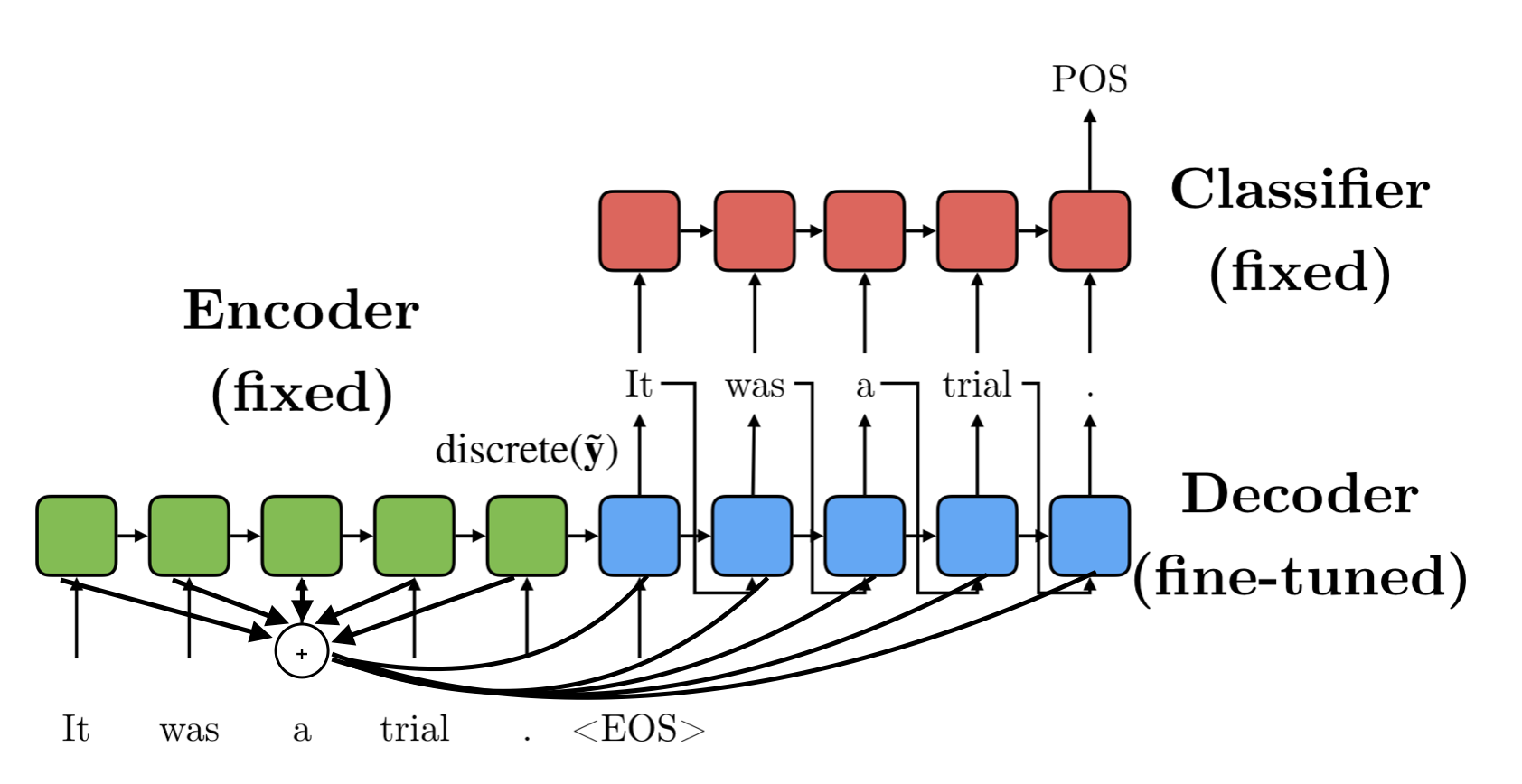
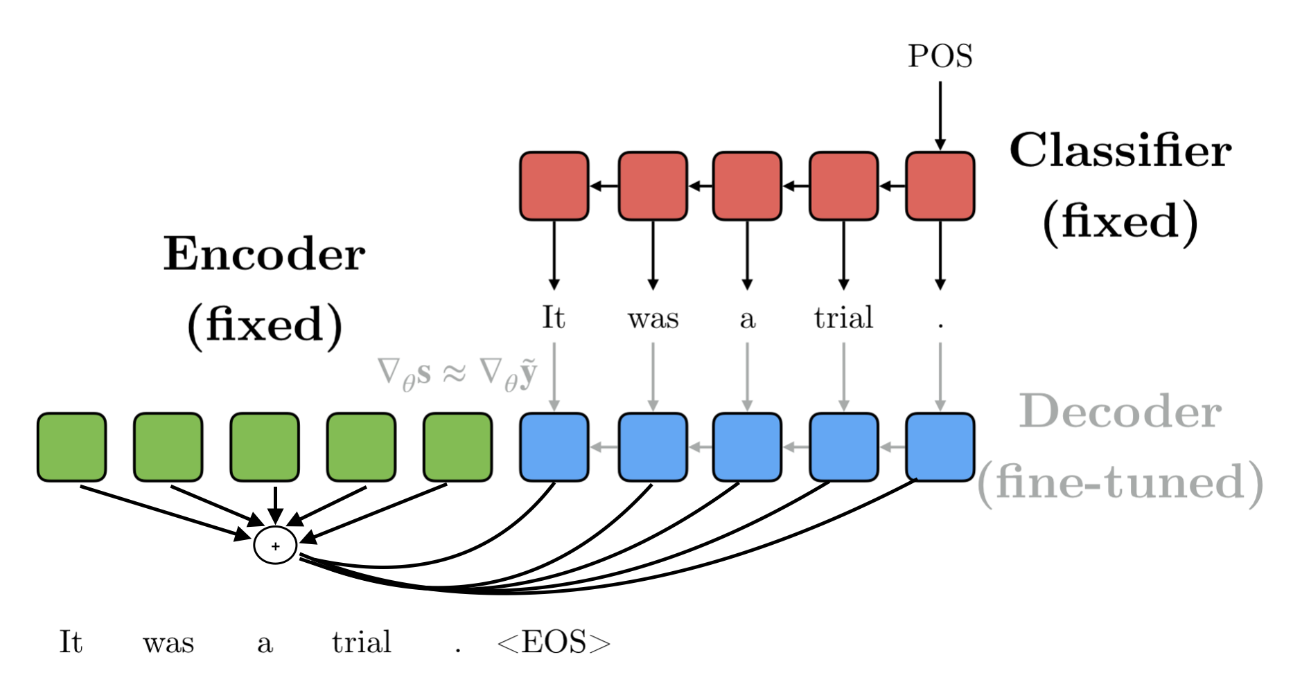
SIFT passes the output of an autoencoder (AE) into a pretrained classifier with frozen weights. We fine-tune the AE with the gradients from the classifier using the Straight-Through Gumbel-Softmax estimator Jang et al. (2017).
During fine-tuning, the AE learns to reformulate parts of the input that are irrelevant to the classifier and to only retain information that it deems useful. Inspecting the reconstructed samples thus gives us a window into what the classifier likes to read.
In contrast to extractive approaches, SIFT is able to leverage information from large amounts of unlabelled data via pretraining, allowing us to make use of a broader vocabulary of words and knowledge for model introspection.
Contributions
We conduct a multi-pronged analysis of three popular sentence classification models—an LSTM-based text classifier, a CNN variant Kim (2014) and a Deep Averaging Network (DAN; Iyyer et al., 2015)—to facilitate comparison between their preferences (§4.1). We are able to extract patterns, which are correlated with the respective model architecture. In an attempt to extract propensities of the pre-trained classification models, we
uncover terms and phrases whose presence in the input causes the classifier to predict a given class (§4.2). Besides the sentence classification tasks, we additionally report results for a two-sentence setup on Natural Language Inference with the model of Bowman et al. (2015).
In all cases we implement simple models and focus on uncovering fundamental dependencies instead of trying to disentangle the various moving parts in more complex models.
2 Related work
Understanding neural networks
Most recent research on understanding neural networks utilizes challenge sets, test suites that seek to evaluate particular properties of a model; see Belinkov and Glass (2019) for an overview. Among these, Adi et al. (2017) investigate if different sentence representations can encode sequence length, word content, and order, while Conneau et al. (2018) test for simple syntactic properties such as constituency tree depth, tense, and subject number.
Zhu et al. (2018) generate triplets of sentences to explore how changes in the syntactic structure or semantics affect the similarities between the embeddings.
Peters et al. (2018) use part-of-speech tagging and constituency parsing for probing contextual representations at different layers.
The drawback of these challenge sets is that they only allow for inspecting characteristics that have to be defined a priori.
A contrasting approach is to investigate the behaviour of individual neurons Li et al. (2016); Bau et al. (2019). This process, however, can quickly become cumbersome as the role of individual neurons differs between models and only yields local insights.
In contrast, our model produces reformulations at a global level for the target model making it easier to inspect. Our model is inspired by the work of Palacio et al. (2018) who also fine-tune an AE with a fixed classifier. Their model however, is only able to deal with continuous inputs and outputs. On the other had, our model learns to reconstruct discrete sequences.
Interpreting model predictions
Much work on interpreting model predictions focuses on extracting rationales—subsets of words from the input that are short, coherent, and suffice to produce a prediction.
Lei et al. (2016) jointly train a generator with the model and extract rationales by forcing the model’s prediction based on the rationale to be close to the model’s prediction on the original input. Ribeiro et al. (2016) propose LIME, which approximates a model locally with a sparse linear model, focusing on keywords that are strongly associated with a class. Ribeiro et al. (2018) propose Anchors, high-precision rules that represent local, ’sufficient’ conditions for predictions and an algorithm to compute them for black-box models. Murdoch et al. (2018) proposes contextual decomposition, a method to decompose the output of LSTMs and identify words and phrases that are associated with different classes.
Bao et al. (2018) use annotated rationales as supervision for attention.
In contrast to these approaches, our method is not limited to extracting words or phrases from the input, but learns to paraphrase and condense relevant information.
Of these extractive methods, the methods by Lei et al. (2016) and Bastings et al. (2019) are most similar to ours as they also train a generator in tandem with a model.
Our approach can also be seen as a way to elicit desired behaviour from an algorithm, similar to Buck et al. (2018) who learn to reformulate questions. While their method is restricted to question answering, our framework is potentially applicable to any arbitrary NLP task.
Data set artifacts
Recent work has shown that data set artifacts, which are introduced as a by-product of crowd-sourced annotations, leak information about the target label Gururangan et al. (2018); Poliak et al. (2018); Tsuchiya (2018). Machine learning algorithms are able to exploit these artifacts to predict the correct class without actually solving the task at hand Sakaguchi et al. (2019). Recent works mostly apply adversarial filtering approaches Zellers et al. (2018); Sakaguchi et al. (2019) to reduce the consequences of the aforementioned bias but have not focused on identifying the artifacts that have been encoded by the model, which we investigate in this work.
3 SIFT
Our proposed Susceptibility Identification through Fine-Tuning (SIFT) framework can be used to analyze any sentence-level pre-trained model. It consists of two stages: Pretraining and Fine-tuning.
Pretraining
We define our autoencoder as an LSTM-based sequence-to-sequence model Sutskever et al. (2014) augmented with attention Bahdanau et al. (2015) that is trained to reliably reconstruct the 1B Word Benchmark Chelba et al. (2013) and the IMDb movie review dataset Maas et al. (2011). We initialize the word embeddings of all models (both AEs and classifiers) with the top 30k 100-dimensional GloVe embeddings Pennington et al. (2014). The encoder (bidirectional, hidden size ) and decoder (uni-directional, hidden size ) of the AE both have one layer.
The encoder’s last hidden states are maxpooled to initialize the decoder.
Prior to fine-tuning, we make a preliminary run of the trained AE on data from the respective classification task in order to adapt it.
Fine-tuning the AE
To achieve our objective of deducing preferences of the classifier,
we fine-tune the decoder of our pre-trained AE using gradients from the pre-trained classifier. We hypothesize that this would have the effect of bring the text produced by the decoder into a form that makes it more amenable to the specific classifier, thus revealing its preferences and idiosyncrasies.
In order to update the parameters of the decoder, we must propagate the gradient through the non-differentiable operation of sampling from a categorical distribution. To overcome this, we employ the Straight-Through Gumbel-Softmax estimator Jang et al. (2017) defined as:
(1)
(a) Autoencoder fine-tuning (forward pass)
(b) Autoencoder fine-tuning (backward pass)
Figure 1: Fine-tuning the decoder of the AE with the gradients of the fixed classifier. During the forward pass (a), the Gumbel-Softmax sample of the AE is discretized
as input for the classifier. During the backward pass (b), gradients are back-propagated through the classifier, through the generated output—using the gradient of the Gumbel-Softmax estimator—to the decoder. Arrows indicate how the gradient is propagated; only parameters with gray arrows are updated.
where is the target position of vocabulary , are logits from the final layer, is a temperature parameter, and corresponds to samples from the Gumbel distribution
with being the uniform distribution. As , the softmax becomes an and the Gumbel-Softmax distribution approximates more closely the categorical distribution.
During the forward pass as shown in Figure 1(a), we discretize this continuous sample using
which is then used to lookup the corresponding word embedding to be passed forward to the classifier.
During the backward pass depicted in Figure 1(b), we approximate the gradient of the discrete sample with the gradient of our continuous approximation .
We found the fine-tuning of the decoder to be extremely sensitive to the choice of hyper-parameters and find that a learning rate of and Gumbel-Softmax temperature of work well for most tasks. We found that including word dropout Iyyer et al. (2015) on the output of the decoder greatly improved stability of training.
4 Experimental Setup
We perform experiments on three sentence classification tasks:
1) Sentiment analysis
(SST-2; Socher et al., 2013);
2) Natural language inference,
(SNLI; Bowman et al., 2015); and
3) PubMed classification
(PubMed; Dernoncourt and Lee, 2017).
We ensure that the pre-trained AE achieves token-level accuracy on the respective data sets establishing that it is able to adequately reproduce the input in the initial pretraining phase.
Orig
<u> turns in a <u> screenplay that <u> at the
edges ; it ’s so clever you want to hate it .
DAN
<u> turns in a <u> screenplay screenplay
screenplay of <u> edges edges edges shapes so
clever easy want hate hate hate hate hate hate
hate hate hate hate
\hdashlineCNN
she turns on a on ( ( in in the the the edges ’s so
clever “ want to hate it ”
\hdashlineRNN
<u> turns in a <u> screenplay was <u> <u>
<u> edges edges edges curves <u> clever
clever you want hate hate it .
Table 1: Example sentences of the different classifiers compared to the original on SST-2. We report further examples in the Appendix. <u> use
for <UNK>.
4.1 SIFT for Classifier Inspection
In contrast to Lei et al. (2016) who extract rationales by enforcing a constraint that actively reduces the number of words, we do not impose any prior in an abstractive attempt to understand the model’s preferences.
Using SIFT we observed substantial differences in the text generated by our fine-tuned decoder when trained with each of the different models.
In order to identify differences, we conducted an automated study of the reconstructed text by inspecting changes in the proportion of part-of-speech tags111NLTK Loper and Bird (2002) was used for POS tagging.
and an increase or decrease in word polarity for sentiment compared to the original input. Examples are in Table 1, results in 2 and 3.
RNN
CNN
DAN
Nouns
DT
Verbs
Adj.
Prep.
Punct.
<U>
RNP
Table 2: Part-of-Speech (POS) changes in SST-2: , , and indicate that the number of occurrences have increased, decreased or stayed the same through fine-tuning respectively. The symbols are purely analytic without any notion of goodness. The numbers indicate the changes in percentage points with respect to the original sentence. A score of 0 thus means that fine-tuning has not changed the number of words. The last row indicates the overlap with the extractive RNP approach. We report results for PubMed in the Appendix.
RNN
CNN
DAN
Positive
+
+
+
Negative
+
+
+
Flipped to Positive
+
+
Flipped to Negative
+
+
+
Table 3: Sentiment score changes in SST-2. The numbers indicate the changes in percentage points with respect to the original sentence. The last two rows correspond to the case where negative labels are flipped to positive and vice versa. and indicate that the score increases in positive and negative sentiment.
Similar to the extractive approach of Lei et al. (2016), who actively mask out terms by extracting them, we find that all three classifiers implicitly mask out words. While the RNN primarily employs UNK tokens or repeats previous words, the CNN masks out UNK tokens using determiners or prepositions. In contrast, DAN masks out punctuation and determiners using words indicative of the class label (i.e. nouns, verbs, adjectives). We hypothesize that these patterns stem from the inductive biases of the classifiers. DAN receives a stronger signal by repeating words with a higher sentiment value due to its averaging, while the CNN does not repeat words (thus having the least amount of changes) and removes uninformative words as its max-pooling layer selects only the most important ones.
Similarly, the gates of the LSTM may allow the model to ignore the random and thus noisy UNK embeddings, which enables it to use this token as a masking operation to ignore unimportant words.
To compare our abstractive with an extractive approach (RNP; Lei et al., 2016), we compute the overlap of retained terms in Table 2 (bottom row). We can see that the DAN has the highest overlap, indicating that it retains words, while the CNN and RNN reformulate sentences. These scores highlight the differences of our approach, as our model does not solely extract indicative words, but reformulates the original sentence.
In order to automatically identify if SIFT retains the sentiment of the sentences, we analyze the output using SentiWordNet Baccianella et al. (2010). By considering only adjectives, we obtain a measure of the positive and negative score for each sentence before and after fine-tuning. The difference of these scores averaged over all examples provides us with a sense of whether the fine-tuning increases the polarity of the sentences (Table 3). We see a constant increase in sentiment value in both directions across all three models after fine-tuning demonstrating that the framework is able to pick up on words that are indicative of sentiment. This is especially true in the case of DAN where we see a large increase as the decoder repeatedly predicts words having high sentiment value. Overall, these results indicate that SIFT is able to highlight certain inductive biases of the model and is able to reformulate and amplify the meaning of the original text based on the classifier’s preferences.
4.2 SIFT for Artifact Detection
Much recent work has focused on detecting artifacts, i.e. in data generated and annotated by humans, with findings that suggest supervised models heavily rely on their existence Levy et al. (2015); Gururangan et al. (2018); May et al. (2019). While e.g. pointwise mutual information (PMI) has been used to identify terms indicative of a specific class Gururangan et al. (2018), it is unclear if a model actually encodes these terms.
Intuitively, such terms may be a source of bias if their presence in the input causes the classifier to change its prediction to their respective class.
To uncover these encoded artifacts we fine-tune SIFT on data where the ground truth label of all examples of a particular class are changed to that of the other class, and this is done subsequently in the other direction.
Since the weights of the classifier are fixed during the fine-tuning phase, our framework forces the decoder to update its parameters to produce text that causes the classifier to reverse the label for the data point. To ensure coherent sentences that are comparable to the original versions, we enforce an additional loss that encourages similarity
by penalizing a large cosine distance (cos) between the average embedding of the sentences:
(2)
with X and being the word embeddings of the original and generated sentence of lengths , .
For this setting we apply SIFT to a sentence pair classification task, i.e. SNLI Bowman et al. (2015) and examine the case where we flip the labels of data points from entailment to contradiction.
SST-2
PubMed
Positive
Negative
Objective
Conclusion
PMI
best
too
compare
should
love
bad
investigate
suggest
fun
n’t
evaluate
findings
SIFT
but
nothing
to
larger
come
awkward
whether
confirm
it
lacking
clarify
concluded
\hdashlineAcc
98%
98%
98%
99%
Corr
0.486
0.5415
0.398
0.00089
Table 4: Top 3 PMI and SIFT terms for a subset of classes with SIFT on the RNN model. The second last row depicts the SIFT accuracy on the test set for the flipped label setting. The last row indicates the correlation of the PMI and SIFT list using weighted Kendall’s tau correlation Shieh (1998) .
We compare the most frequent SIFT terms with the most indicative words w.r.t. a class using PMI with 100 smoothing, following Gururangan et al. (2018). We list the most frequently used words in Table 4. To understand how similar the SIFT terms are to the PMI terms we calculate the weighted Kendall’s tau correlation Shieh (1998), which weights terms higher in the list as more important.
In the case of high correlation, we hypothesize that the classifier has memorized the artifacts of the data set, which in turn SIFT has leveraged to “fool” the classifier. This “fooling” in the case of sentiment analysis is due to the terms being indicative of the respective class and having high sentiment (cf. Table 3). For SNLI, we find that many of the top PMI and SIFT terms overlap, and slightly correlate (). We find terms (as reported in Appendix A2), e.g. ‘sleeping’, ‘cats’, ‘cat’, that were identified as artifacts by Gururangan et al. (2018).
In the PubMed task where the aim is to classify sentences as belonging to one of five classes—background, objective, methods, results, conclusions—the top terms in the setting where we change ground truth from “objective” to “conclusion” are intuitively relevant terms for that class. They do not, however, correlate with PMI, which might indicate that pretraining on large unlabelled data has enabled SIFT to capture these relations.
Overall, this shows that SIFT is able to identify both previously known as well as novel artifacts. In contrast to PMI, SIFT uncovers the propensities of the trained model and not only the data set, giving insight into what the model has actually encoded.
5 Conclusion
We have proposed a bottom-up approach for extracting a model’s preferences and consequently understanding opaque neural network architectures better. We have sought to overcome the difficulty of evaluating an abstractive unsupervised approach by means of a multi-pronged analysis, highlighting how our approach can be used to analyze examples, compare classifiers, and generate sentences with opposite labels. We were able to uncover significant differences of what the respective architectures want to read by sifting out what models have encoded in order to understand their limits and create fair representations in the future.
We believe that our approach is an important first step towards abstractive interpretability methods and bottom-up bias identification in NLP.
Baccianella et al. (2010)
Stefano Baccianella, Andrea Esuli, and Fabrizio Sebastiani. 2010.
Sentiwordnet 3.0: an enhanced lexical resource for sentiment analysis
and opinion mining.
In Lrec, volume 10, pages 2200–2204.
Bahdanau et al. (2015)
Dzmitry Bahdanau, Kyunghyun Cho, and Yoshua Bengio. 2015.
Neural Machine Translation by Jointly Learning to Align and
Translate.
In Proceedings of ICLR 2015.
Bastings et al. (2019)
Joost Bastings, Wilker Aziz, and Ivan Titov. 2019.
Interpretable
neural predictions with differentiable binary variables.
In Proceedings of the 57th Conference of the Association for
Computational Linguistics, ACL 2019, Florence, Italy, July 28- August 2,
2019, Volume 1: Long Papers, pages 2963–2977.
Bowman et al. (2015)
Samuel R. Bowman, Gabor Angeli, Christopher Potts, and Christopher D. Manning.
2015.
A large annotated corpus for learning natural language inference.
In Proceedings of the 2015 Conference on Empirical Methods in
Natural Language Processing (EMNLP). Association for Computational
Linguistics.
Buck et al. (2018)
Christian Buck, Jannis Bulian, Massimiliano Ciaramita, Wojciech Gajewski,
Andrea Gesmundo, Neil Houlsby, and Wei Wang. 2018.
Ask the Right Questions: Active Question Reformulation with
Reinforcement Learning.
In Proceedings of ICLR 2018.
Chelba et al. (2013)
Ciprian Chelba, Tomas Mikolov, Mike Schuster, Qi Ge, Thorsten Brants, Phillipp
Koehn, and Tony Robinson. 2013.
One billion word benchmark for measuring progress in statistical
language modeling.
arXiv preprint arXiv:1312.3005.
Dernoncourt and Lee (2017)
Franck Dernoncourt and Ji Young Lee. 2017.
Pubmed 200k rct: a dataset for sequential sentence classification in
medical abstracts.
arXiv preprint arXiv:1710.06071.
Gururangan et al. (2018)
Suchin Gururangan, Swabha Swayamdipta, Omer Levy, Roy Schwartz, Samuel R.
Bowman, and Noah A. Smith. 2018.
Annotation artifacts in natural language inference data.
In Proceedings of the 2018 Conference of the North American
Chapter of the Association for Computational Linguistics: Human Language
Technologies, NAACL-HLT, New Orleans, Louisiana, USA, June 1-6, 2018, Volume
2 (Short Papers), pages 107–112.
Iyyer et al. (2015)
Mohit Iyyer, Varun Manjunatha, Jordan L. Boyd-Graber, and Hal Daumé
III. 2015.
Deep
unordered composition rivals syntactic methods for text classification.
In Proceedings of the 53rd Annual Meeting of the Association
for Computational Linguistics and the 7th International Joint Conference on
Natural Language Processing of the Asian Federation of Natural Language
Processing, ACL 2015, July 26-31, 2015, Beijing, China, Volume 1: Long
Papers, pages 1681–1691.
Kim (2014)
Yoon Kim. 2014.
Convolutional
neural networks for sentence classification.
In Proceedings of the 2014 Conference on Empirical Methods in
Natural Language Processing, EMNLP 2014, October 25-29, 2014, Doha, Qatar,
A meeting of SIGDAT, a Special Interest Group of the ACL, pages
1746–1751.
Lei et al. (2016)
Tao Lei, Regina Barzilay, and Tommi Jaakkola. 2016.
Rationalizing Neural
Predictions.
In Proceedings of EMNLP 2016.
Levy et al. (2015)
Omer Levy, Steffen Remus, Chris Biemann, and Ido Dagan. 2015.
Do supervised distributional methods really learn lexical inference
relations?
In Proceedings of the 2015 Conference of the North American
Chapter of the Association for Computational Linguistics: Human Language
Technologies, pages 970–976.
Li et al. (2016)
Jiwei Li, Xinlei Chen, Eduard H. Hovy, and Dan Jurafsky. 2016.
Visualizing
and understanding neural models in NLP.
In NAACL HLT 2016, The 2016 Conference of the North
American Chapter of the Association for Computational Linguistics: Human
Language Technologies, San Diego California, USA, June 12-17, 2016, pages
681–691.
Loper and Bird (2002)
Edward Loper and Steven Bird. 2002.
Nltk: the natural language toolkit.
arXiv preprint cs/0205028.
Maas et al. (2011)
Andrew L. Maas, Raymond E. Daly, Peter T. Pham, Dan Huang, Andrew Y. Ng, and
Christopher Potts. 2011.
Learning word
vectors for sentiment analysis.
In The 49th Annual Meeting of the Association for Computational
Linguistics: Human Language Technologies, Proceedings of the Conference,
19-24 June, 2011, Portland, Oregon, USA, pages 142–150.
Palacio et al. (2018)
Sebastian Palacio, Joachim Folz, Jörn Hees, Federico Raue, Damian Borth,
and Andreas Dengel. 2018.
What do Deep
Networks Like to See?In Proceedings of CVPR 2018.
Pennington et al. (2014)
Jeffrey Pennington, Richard Socher, and Christopher D. Manning. 2014.
Glove: Global Vectors
for Word Representation.
In Proceedings of the 2014 Conference on Empirical Methods in
Natural Language Processing, pages 1532–1543.
Poliak et al. (2018)
Adam Poliak, Jason Naradowsky, Aparajita Haldar, Rachel Rudinger, and Benjamin
Van Durme. 2018.
Hypothesis only baselines in natural language inference.
In Proceedings of the Seventh Joint Conference on Lexical and
Computational Semantics, pages 180–191.
Ribeiro et al. (2016)
Marco Tulio Ribeiro, Sameer Singh, and Carlos Guestrin. 2016.
”Why Should I Trust You ?” Explaining the Predictions of Any
Classifier.
In Proceedings of the 22nd ACM SIGKDD International Conference
on Knowledge Discovery and Data Mining. ACM.
Ribeiro et al. (2018)
Marco Tulio Ribeiro, Sameer Singh, and Carlos Guestrin. 2018.
Anchors: High-Precision Model-Agnostic Explanations.
In Proceedings of AAAI 2018.
Sakaguchi et al. (2019)
Keisuke Sakaguchi, Ronan Le Bras, Chandra Bhagavatula, and Yejin Choi. 2019.
Winogrande: An adversarial winograd schema challenge at scale.
arXiv preprint arXiv:1907.10641.
Shieh (1998)
Grace S Shieh. 1998.
A weighted kendall’s tau statistic.
Statistics & probability letters, 39(1):17–24.
Socher et al. (2013)
Richard Socher, Alex Perelygin, Jean Wu, Jason Chuang, Christopher D. Manning,
Andrew Y. Ng, and Christopher Potts. 2013.
Recursive
deep models for semantic compositionality over a sentiment treebank.
In Proceedings of the 2013 Conference on Empirical Methods in
Natural Language Processing, EMNLP 2013, 18-21 October 2013, Grand Hyatt
Seattle, Seattle, Washington, USA, A meeting of SIGDAT, a Special Interest
Group of the ACL, pages 1631–1642.
Sutskever et al. (2014)
Ilya Sutskever, Oriol Vinyals, and Quoc V Le. 2014.
Sequence to sequence learning with neural networks.
In Z. Ghahramani, M. Welling, C. Cortes, N. D. Lawrence, and K. Q.
Weinberger, editors, Advances in Neural Information Processing Systems
27, pages 3104–3112. Curran Associates, Inc.
Tsuchiya (2018)
Masatoshi Tsuchiya. 2018.
Performance impact caused by hidden bias of training data for
recognizing textual entailment.
In Proceedings of the Eleventh International Conference on
Language Resources and Evaluation (LREC-2018).
Zellers et al. (2018)
Rowan Zellers, Yonatan Bisk, Roy Schwartz, and Yejin Choi. 2018.
Swag: A large-scale adversarial dataset for grounded commonsense
inference.
In Proceedings of the 2018 Conference on Empirical Methods in
Natural Language Processing, pages 93–104.
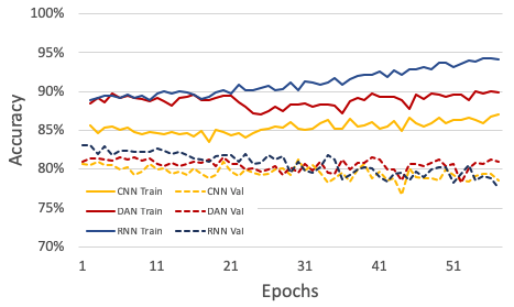
Figure 2: Train and validation accuracy of SIFT in the Classifier Inspection setting for CNN, RNN, and DAN models on SST-2.
RNN
CNN
DAN
Nouns
DT
Verbs
Adj.
Prep.
Punct.
<U>
Table A1: Part-of-Speech (POS) changes in PubMed: , , and indicate that the number of occurrences have increased, decreased or stayed the same through fine-tuning respectively. The numbers indicate the changes in percentage points wrt to the original sentece. A score of 0 would thus mean that fine-tuning has not changed the number of words.
SNLI
Neutral
Contradiction
PMI
winning
nobody
vacation
cats
favorite
sleeping
sad
cat
owner
tv
SIFT
one
sitting
out
cave
batman
women
on
hand
with
one
\hdashlineAccuracy
30%
70%
Corr
-0.0059
0.366
Table A2: Top 5 PMI and SIFT terms for SNLI in the Artifact Detection setting. The second last row depicts the SIFT accuracy on the test set for the one class, flipped label setting. The last row indicates the correlation of the PMI and SIFT list using weighted Kendall’s tau correlation Shieh (1998). Note that this setting is very difficult for the current SIFT architecture as the decoders do not have access to the information of the paired sentence. While Entailment to Contradiction works well reaching accuracy, Contradiction to Neutral is only able to fool the classifier in of the cases. We hypothesize that the good results for Entailment to Contradiction result from the fact that for a sentence pair and , if we find a reformulation such that contradicts , will most likely also contradict . Thus the decoder simply needs to generate a sentence which contradicts its input.
O P
adults with their kids are riding on a small red train .
G P
adults with people are riding small are train on on sleeping on on
H
there are people on the train .
O P
a black and white dog running through shallow water .
G P
with black white cat it water a small bed a on surface water
H
two dogs running through water .
O P
two boys in green and white uniforms play basketball with two boys in blue and white
uniforms .
G P
with girls in white uniforms . and girls black white women in women black cats black sitting
two
H
two different teams are playing basketball .
O P
very large group of old people riding in boats down a river .
G P
the small large group old riding boats the in in sitting a on on
H
mob of elderly riding water crafts .
Table A3: Examples of premise sentences generated when controlled to produce a contradiction from and entailment with O standing for Original, G for generated H for Hypothesis and P for Premise. In this setting we only fine-tune the Premise as to not confuse SIFT by moving two independent parts. We highlight the terms we find most likely have fooled the classifier. Although many sentence pairs do not actually contradict each other, the classifier labels it as such, indicating that it has fixated on artifacts i.e. ‘sleeping’, ‘cats’, ‘sitting’
Orig
it ’s a great deal of <u> and very little steak .
DAN
it ’s ’s great yet of <u> and very good makes while
\hdashlineCNN
it ’s a great it of it and very good it . <u> . a . makes , so
\hdashlineRNN
it ’s a great deal of <u> and very good sweet .
Orig
fails to bring as much to the table .
DAN
fails help bring as much to the coming .
\hdashlineCNN
take to bring it this to at you <u> . a . makes , so
\hdashlineRNN
manages to bring as much to the table .
Orig
now it ’s a bad , embarrassing movie .
DAN
now it ’s a bad , embarrassing movie .
\hdashlineCNN
now it ’s a good , enough movie . this it makes it makes , makes , makes <u> . a . makes , so
\hdashlineRNN
now it ’s a good , unexpected movie .
Orig
an often - deadly boring , strange reading of a classic whose witty dialogue is treated with a
<u> casual approach
DAN
an often - full boring , strange reading of a theme whose witty dialogue is treated with a
<u> casual yet
\hdashlineCNN
an often - a pleasant , strange reading of a classic whose charming dialogue is taking with a
. life
\hdashlineRNN
an often - deadly hilarious , strange reading of a classic whose witty dialogue is treated with
a <u> perspective come
Orig
a gimmick in search of a movie : how to get <u> into as many silly costumes and deliver as
many silly voices as possible , plot mechanics be damned .
DAN
a gimmick in search of a theme : see to get <u> into as many good costumes and deliver as
many good voices as possible , plot mechanics be damned while
\hdashlineCNN
a offers in search of a film : how to take <u> up also many fun costumes and deliver also
many good and as this , one skills be this this on to a . makes often
\hdashlineRNN
a riveting in connection of a movie : how to get <u> into as many silly costumes and deliver
as many silly voices as possible , plot mechanics be damned come
Table A4: Example output for SIFT in the Artifact Detection setting of the different classifiers compared to the original on SST-2. In this case we have flipped the labels from negative to positive.
Orig
invincible is a wonderful movie .
DAN
invincible is a wonderful movie however
\hdashlineCNN
this is a little movie
\hdashlineRNN
wes is a pathetic movie .
Orig
sharp , lively , funny and ultimately sobering film .
DAN
sharp , lively , funny and ultimately sobering film .
\hdashlineCNN
and , little , little and which this film
\hdashlineRNN
sharp , awkward , joke and ultimately puzzling film .
Orig
an exciting and involving rock music doc , a smart and satisfying look inside that
tumultuous world .
DAN
an interesting and involving rock music doc , another wise and satisfying things inside that
tumultuous series however
\hdashlineCNN
an course and this rock music doc , a little and kind even inside that half this .
\hdashlineRNN
an boring and involving rock music doc , a smart and predictable looking inside that
dilapidated world .
Table A5: Example output for SIFT in the Artifact Detection setting of the different classifiers compared to the original on SST-2. In this case we have flipped the labels from positive to negative.
Orig
rates an ‘ e ’ for effort – and a ‘ b ’ for boring .
DAN
rates ‘ e e effort effort – – – ‘ b b b boring boring boring boring boring
\hdashlineCNN
rates on ‘ bad on on on in in in ’ an ‘ ’ a boring ”
\hdashlineRNN
rates called ‘ 8 <u> from <u> while , of ‘ b b of boring boring
Orig
if your senses have n’t been <u> by <u> films and <u> , if you ’re
a <u> of psychological horror , this is your ticket .
DAN
if senses senses have n’t n’t been <u> <u> <u> films films films , <u> , you ’re
psychological psychological horror this is your ticket ticket ticket ticket
\hdashlineCNN
but your how hard out on in in in ( ( ( ( ( ( ( on about about about about horror this this
your ticket ”
\hdashlineRNN
it your desire <u> n’t been <u> by <u> <u> , <u> , <u> you you <u> <u> of
psychological horror , this is your bet bet limit limit
Orig
<u> turns in a <u> screenplay that <u> at the edges ; it ’s so clever you want to hate it .
DAN
<u> turns in a <u> screenplay screenplay screenplay of <u> edges edges edges shapes
so clever easy want hate hate hate hate hate hate hate hate hate hate
\hdashlineCNN
she turns on a on ( ( in in the the the edges ’s so clever “ want to hate it ”
\hdashlineRNN
<u> turns in a <u> screenplay was <u> <u> <u> edges edges edges curves <u> clever
clever you want hate hate it .
Orig
a pleasant <u> through the sort of <u> terrain that <u> morris has often dealt with … it
does possess a loose , <u> charm .
DAN
a pleasant <u> through the sort kind <u> terrain terrain terrain terrain <u> morris
a pleasant <u> through on on in in ( ( ( ( ( ( ( on on that that about about about a <u>
charm ”
\hdashlineRNN
a pleasant <u> through the idea of <u> woven of <u> <u> <u> often <u> <u>
<u> which may can a loose , <u> wit charm
Table A6: Example output for SIFT in the Classifier Inspection setting of the different classifiers compared to the original on SST-2. We can see that DAN keeps repeating words that have high sentiment value. CNN masks out words with ‘(’ and stop-words (‘about’, ‘on’, etc.). RNN uses <u> or repeats previous words as masking operators.
Orig
there was no significant difference in overall survival between groups ( median overall
survival 128 months [ <u> % ci 105 - 143 ] in the <u> group vs 143 months [ 125 - 165 ]
in the <u> and <u> group ; hazard ratio [ hr ] <u> [ <u> % ci <u> - 103 ] ; <u> log -
rank test p = <u> ) .
DAN
there was no significant difference by overall survival between groups ( median overall
individual [ [ [ <u> % ci 105 - 143 ] in the <u> group vs 143 months [ 125 - 165 ] in the
<u> and <u> group ; hazard ratio [ hr ] <u> [ <u> % ci <u> - 103 ] ; <u> log - rank
test p = <u> ) .
\hdashlineCNN
there was no significant difference in overall survival between groups : median overall [ =
- - - , , ] , , ] <u> <u> group group , 161 months [ 125 - 165 ] in the <u> and <u> group ;
hazard ratio [ hr ] <u> [ <u> % ci <u> - 103 ] ; <u> log - rank test p = <u> ) .
\hdashlineRNN
there was no significant difference in overall survival <u> <u> - <u> <u> <u> <u> vs
<u> - <u> ] in the <u> group vs <u> <u> [ 125 - 165 ] in the <u> and <u> group ;
<u> group <u> hazard ratio hr ] <u> [ <u> <u> ci <u> ci <u> <u> - <u> ] ; <u>
log - rank p = <u>
Orig
study 1 : under <u> conditions , a separation between <u> and placebo on minute
ventilation was observed by 6.1 ( 3.6 to 8.6 ) l / min ( p < 0.01 ) and 3.6 ( 1.5 to 5.7 ) l / min
( p < 0.01 ) at low - dose <u> plus high - dose <u> and high - dose - <u> plus high - dose
DAN
study 1 or by <u> conditions , a separation between <u> and placebo on minute
ventilation was observed by mis ( 3.6 to 8.6 ) l / min ( p < 0.01 ) and 3.6 ( 1.5 to 5.7 ) l / min
( p < 0.01 ) at low - dose <u> plus high - dose <u> and high - dose - <u> plus high - dose
\hdashlineCNN
study 1 : under <u> conditions , a separation between <u> and placebo at 8.2 , : 3.6 ,
3.6 , 3.4 ) = , l , min , p < 0.01 ) and 3.6 ( 1.5 to 6.3 ) l / min ( p < 0.01 ) at low - dose <u>
plus high - dose <u> and high - dose - <u> plus high - dose
\hdashlineRNN
study 1 : by <u> conditions , a <u> and <u> and <u> - <u> , , <u> <u> min / min ,
min , <u> min , p < 0.01 , and 3.6 - 1.5 - <u> <u> min / min ( p < 0.01 ) at low - dose
<u> plus high - <u> <u> and high - dose - <u> plus <u> -
Table A7: Example output for SIFT in the Classifier Inspection setting of the different classifiers compared to the original on PubMed. Similar to SST-2 we can see that CNN masks out words with punctuation and RNN uses <u>.