Differential equations as models of deep neural networks
Abstract
In this work we systematically analyze general properties of differential equations used as machine learning models. We demonstrate that the gradient of the loss function with respect to to the hidden state can be considered as a generalized momentum conjugate to the hidden state, allowing application of the tools of classical mechanics. In addition, we show that not only residual networks, but also feedforward neural networks with small nonlinearities and the weights matrices deviating only slightly from identity matrices can be related to the differential equations. We propose a differential equation describing such networks and investigate its properties.
Baltic Institute of Advanced Technology (BPTI), Pilies 16-8, LT-01403,
Vilnius, Lithuania
julius.ruseckas@bpti.lt
1 Introduction
Deep learning is a form of machine learning that uses neural networks with many hidden layers [1, 2]. Deep learning models have dramatically improved speech recognition, visual object recognition, object detection and many other domains [2]. Since the number of layers in deep neural networks become large, it is possible to consider the layer number as a continuous variable [3] and represent the neural network by an differential equation.
The connection between the neural networks and differential equations first appeared with an additive model for continuous time recurrent neural networks, described by the differential equations [4]
| (1) |
Cohen and Grossberg applied the Liapunov method to prove that global limits exist in a class of dynamical systems with symmetric interaction coefficients, which includes the additive and shunting models [5]. Hopfield’s work [6] pioneered the analog computation of continuous time recurrent neural networks instead of digital computation using complex numerical algorithms on a digital computer. A Hopfield network has a quadratic form as an Lyapunov function for the activity dynamics. As a consequence, the state of the network evolves to a final state that is a minimum of the Lyapunov function when started in any initial state [7]. Continuous time recurrent neural networks have been applied to address vision [8], cognitive behavior [9], and cooperation [10].
New relations between neural network and differential equation appeared after proposal of residual networks (ResNets) [11]. Forward propagation of discrete vector through residual network can be written as
| (2) |
where are the parameters that need to be determined by the training of the neural network. In [12] a connection of residual network with recurrent neural network, which is known as an approximation of a dynamical system, has been made. Furthermore, equation (2) can be seen as an Euler discretization
| (3) |
of an ordinary differential equation (ODE)
| (4) |
Such a link between residual neural networks and nonlinear differential equations has been first proposed in [13, 14]. This interpretation of neural network as a discretization of differential equation has been applied to analyze stability properties of deep learning [15] and to derive reversible neural network architectures [16]. The view of ResNets as an Euler discretization of ODEs allowed to construct invertible ResNets (i-ResNets) [17]. Related to this interpretation is a view of a finite deep neural network as a broken line approximation of a continuous trajectory [3] and the formulation of the training process of ResNet as an control problem of a transport equation [18]. Subsequently it has been demonstrated [19] that many networks, such as ResNet, PolyNet, FractalNet and RevNet, can be interpreted as different numerical discretizations of differential equations and linear multi-step architecture has been proposed. In addition to interpreting the layer depth as a continuous variable, the input to the neural network can also be represented as being continuous. Such a view has been taken in [20], where residual convolutional neural networks have been interpreted as a discretization of a space-time partial differential equation (PDE). In [21, 22] a new feed-forward deep network, PDE-Net, has been proposed to predict dynamics of complex systems and to uncover the underlying hidden PDE models. Further connection between RNNs and ODEs has been revealed in [23]. It has been shown that the temporal dynamics of RNN architectures can be represented by a specific numerical integration method for ODEs of a given order.
Using differential equations a family of models called Neural ODEs has been proposed in [24]. The output of the network is computed using a black-box differential equation solver and the gradients are computed by solving a second, augmented ODE backwards in time [24]. These models have shown great promise on a number of tasks including modeling continuous time data and building normalizing flows with low computational cost. In particular, ODEs have been applied to model time series with non-uniform intervals by generalizing state transitions in RNNs to continuous-time dynamics [25]. However, neural ODEs learn representations that preserve the topology of the input space, therefore there exist functions that neural ODEs cannot represent [26]. Usual ResNets, being a discretization of the ODE, allow the trajectories to make discrete jumps to cross each other and do not have this limitation. To address the limitations of neural differential equations, Augmented Neural ODEs are introduced by adding additional dimensions [26].
In this work we first systematically analyze general properties of differential equations used as machine learning models. We demonstrate that the gradient of the loss function with respect to to the hidden state can be considered as a generalized momentum conjugate to the hidden state, allowing application of the tools of classical mechanics. In addition, we show that not only residual networks, but also feedforward neural networks with small nonlinearities and the weights matrices deviating only slightly from identity matrices can be related to the differential equations. We propose a differential equation describing such networks and investigate its properties.
This paper is organized as follows. In section 2 we investigate general properties of first-order nonlinear differential equations as models in machine learning. In section 3 we propose a differential equation describing feedforward neural networks and in section 4 we analyze its properties. In section 5 we apply the proposed differential equation for a couple of simple problems. Finally, section 6 summarizes our results.
2 Ordinary differential equations as machine learning models
In this section we investigate nonlinear ordinary differential equations used as machine learning models. We assume the differential equations of the form
| (5) |
where are nonlinear functions and are arbitrary parameters that are functions of . Equation (5) is more general than the differential equations considered in [24], where the parameters do not depend on . Starting from the input , the output is the solution at to the initial value problem of the differential equation (5). The output corresponds to the features learned by the model. The parameters are adjusted such that equation (5) transforms the input to a which is close to true label .
2.1 Backward propagation for differential equations
Let us consider a loss function that is a function of a final output . The minimum of the loss can be found by applying the gradient descent method. When is a continuous variable, the loss function is a functional of functions and should be minimized with the constraint , where for the brevity we use the notation . A general method how to find such a minimum by introducing backpropagating dynamics is given by Pontryagin’s minimum principle [27]. In this section we briefly sketch the derivation of the backpropation corresponding to equation (5). In order to derive update rule for for the parameters one needs to use calculus of variations and compute the functional derivatives [28]. For the minimization with constraints we can employ the method of Lagrange multipliers. Thus we will consider the functional
| (6) |
where is a vector of Lagrange multipliers. Since the constraint is satisfied by construction, we are free to set the values of . We need to calculate the functional derivative . Using equation (6) we obtain
| (7) |
The last term we integrate by parts:
| (8) |
The initial condition does not depend on the parameters , therefore . Inserting into equation (7) we have
| (9) |
Since can be arbitrary, we can set the coefficients in equation (9) to be zero:
| (10) |
and
| (11) |
Equation (11), representing the differential equation for backward propagation, is adjoint to the equation (5) [27]. It is a continuous-time analog to the usual backporpagation algorithm [29]. In contrast to the non-linear equation (5) for the forward propagation, equation (11) for the backward propagation of the gradient is linear. The remaining term in equation (9) gives
| (12) |
An alternative derivation of equation (11) that does not involve variational calculus is presented in the Appendix A.
If the functions depend on parameters that do not depend on , , then the gradient of the loss can be calculated as
| (13) |
Using equation (12) we get
| (14) |
In particular, if the parameters do not depend on then we can take and from equation (14) obtain
| (15) |
The total time can also be interpreted as one of the parameters of the model. The gradient of the loss with respect to the total time is
| (16) |
2.2 Euler-Lagrange and Hamiltonian form of the equations
Equations (5) and (11) can be written in the form of the Euler-Lagrange equations
| (17) | ||||
| (18) |
with the Lagrangian
| (19) |
Here and play the role of generalized coordinates. Lagrangian of this type for differential equations considered together with adjoint equations has been proposed in [30]. This Lagrangian (19) appears in equation (6). The Lagrangian (19) yields the generalized momentum
| (20) |
leading to the corresponding Hamiltonian
| (21) |
Then the equations (5) and (11) take the form of the Hamilton equations
| (22) | ||||
| (23) |
The Hamiltonian (21) is the same as in Pontryagin’s principle [27].
2.3 Probability density functions
Let us assume that initial data is characterized by a probability density function . The solution of the differential equation (5) has a transformed probability density . Since the transformation of the variable is described by a differential equation, the probability density obeys the continuity equation [3]
| (26) |
Computing partial derivatives we obtain the partial differential equation
| (27) |
This equation can be written in the form of the instantaneous change of variables formula of [24]:
| (28) |
Now let us consider the probability density of features together with the gradient of the loss. From the existence of the Hamiltonian follows that the Liouville’s theorem holds: the total derivative of the probability density function is zero:
| (29) |
or, explicitly,
| (30) |
The distribution is constant along any trajectory in phase space .
The information entropy associated with the data is defined as
| (31) |
Since obeys the differential equation (27), for the information entropy we have
| (32) |
With increasing the model should discard the features that are unnecessary for the prediction of true label . Thus one can argue that the information entropy should decrease with , . This also follows from the requirement of the stability of differential equations (5) [15].
2.4 Symmetric equations
Let us consider the case where the function satisfies the condition
| (33) |
that is, the matrix is symmetric. Then the vector field is conservative and, therefore, it can be expressed as a gradient of of scalar function:
| (34) |
In such a case the differential equation (5) can be written as
| (35) |
If the parameters do not depend on , the function does not increase with with . Indeed, we have
| (36) |
The existence of an energy function that decrease along trajectories is a property of Cohen-Grossberg model [5] and Hopfield’s [6] continuous time recurrent neural networks.
2.5 Gradient descent updates of the parameters
If the parameters are changed by , the change of the loss function due to the change of the parameters is
| (37) |
Let us find the optimal updates of the parameters in the gradient descent step, leading to a largest change of the loss. In order to fix a learning rate we will keep the norm of fixed, . Then the optimal change can be found using Lagrange multipliers by maximizing the functional
| (38) |
This gives the optimal change
| (39) |
leading to the change of the loss function
| (40) |
Using equation (12) we get the updates of the parameters in the gradient descent step
| (41) |
When the function is parameterized by parameters , then the change is
| (42) |
with
| (43) |
The change of the loss function becomes
| (44) |
In particular, if the parameters do net depend on then
| (45) |
and the change of the loss function is
| (46) |
One can see that in the equation (40) the integral is taken of the non-negative quantity. Each infinitesimal segment has a positive contribution to the change of the loss. On the other hand, in equation (46) the integration is performed of the quantities that can have various signs and different segments of can partially cancel each other, resulting in smaller change of the loss. The parameters that depend on can lead to faster training of the model.
3 Ordinary differential equation as a model of feedforward neural networks
3.1 Heuristic derivation of differential equation
In this section we present a non-strict derivation of a differential equation that captures essential properties of feedforward neural networks. Let us consider a feedforward neural network consisting of a large number of layers. The -th layer () applies a nonlinear transform on its input to produce its output , where the nonlinear transform is an affine transform
| (47) |
followed by a non-linear activation function :
| (48) |
Here in the equation (47) is a matrix of weights and is a bias vector. For simplicity at first we assume that the vector has the same number of dimensions as ; the situation when the dimensions are different will be discussed below (subsection 3.2). In order to obtain a differential equation we require that the vector differ only slightly from . Small difference between the input and the output of a layer can occur when the matrix has the form
| (49) |
where is an identity matrix and is a small parameter. In addition, the bias also should be proportional to the small parameter,
| (50) |
In such a case the affine transform reads
| (51) |
Thus the affine transform is a sum of two terms, the first term being an unchanged input and the second term being proportional to the small parameter . The first term resembles a shortcut connection in highway networks [32, 33] and residual networks [11].
Furthermore, to get small difference between the input and the output of a layer, the non-linear function should be almost linear. We can obtain such a nonlinear function by adding a small cubic term to the linear function:
| (52) |
where is a parameter of nonlinearity. One can interpret this non-linear function as a generalization of a hyperbolic tangent activation, because the first two terms in the Taylor series of are . Note, that Taylor series of arbitrary function should have also a quadratic term , however the quadratic term can be eliminated by the shift of . If one considers non-analytic functions, equation (48) can be generalized as
| (53) |
where is the exponent of nonlinearity.
Combining the equations (48), (51), (52) and keeping only the terms up to the first order in we obtain
| (54) |
Instead of the layer number we will use and write instead of , rewriting the equation (54) as
| (55) |
Interpreting as a continuous variable and taking the limit we obtain a differential equation
| (56) |
Note, that the equation (56) is non-linear, the non-linear term plays the role of a non-linear activation function. Using the non-linear activation function (53) the differential equation becomes
| (57) |
Since the non-linear differential equation (56) has been obtained starting from a discrete neural network, we expect that the proposed equation can reflect some properties of deep neural networks.
Equation (56) can be further generalized to the case of continuous indices, yielding an integro-differential equation
| (58) |
Such double continuum limit of neural networks has been proposed in [3]. Taking a singular kernel in equation (58) one can get a partial differential equation instead of an integral one [20, 21, 22].
3.2 Different number of dimensions in input and output
When the number of dimensions in the output differs form the number of dimensions in the input , the structure of the weights (49) is not possible and the transition to the differential equation is not straightforward. However, when the number of dimensions is increased, at some , we can interpret this increase as the presence of units with the activation equal to zero in the -th layer. Then we can require the structure of the weights that can be described by an equation similar to (49), where the identity matrix is replaced by a rectangular matrix with ones on the main diagonal and zeros elsewhere. Equation (54) then becomes
| (59) |
This equation keeps the norm of equal to the norm of when . In the limit we get the differential equation (56) with an additional boundary condition if .
When the number of dimensions in the output is decreased, a rectangular matrix that keeps the norm of a vector equal to the norm of does not exist. Thus decreasing the number of units necessarily leads to the change of the norm of the signal.
3.3 Backward propagation for the proposed model
The general equations obtained in the previous section 2 can be applied to the proposed differential equation (56), which corresponds to the function
| (60) |
Thus,
| (61) |
and the differential equation for the backward propagation becomes
| (62) |
The last term on the right hand side of equation (62) represents a decay of the gradient with the decay rate that increases with increasing signal . In a similar way, starting with the forward propagation equation (57), we get the differential equation
| (63) |
In the case of continuous indices this backward propagation equation has the form
| (64) |
According to the equation (12), the gradients (functional derivatives) of the loss function with respect to the parameters and are
| (65) | ||||
| (66) |
These gradients lead to the updates of the parameters in the gradient descent step
| (67) | ||||
| (68) |
Here the function should be obtained by solving equation (62) first. However, from equations (56) and (62) follows that we can obtain the updates to the parameters and by directly solving the following differential equations:
| (69) | ||||
| (70) |
We can consider the parameter of nonlinearity as an additional parameter to be learned instead of having a fixed value. The learnable parameter of nonlinearity is similar to the idea of Parametric ReLUs [34]. From the equation (15) we can obtain the gradient of the loss with respect to the parameter :
| (71) |
3.4 Convolutional neural networks
Equation (56) can be easily adapted to model convolutional neural networks. For convolutional neural networks the affine transformation (47) reads
| (72) |
Here for simplicity we write the equation as one-dimensional cross-correlation with only one feature channel. The generalization to more dimensions and more channels is straightforward. In addition, we assume that input is zero padded so that the size of the output is the same as the size of the input. Requiring that
| (73) |
and
| (74) |
in the limit we obtain the differential equation
| (75) |
When there are more than one channel we assume that the number of channels in each layer remains the same. In this case the forward propagation is described by differential equations that are similar to the equations (75), only with summation over channels added.
Proceeding similarly as in subsection 3.3, from equation (75) we get the differential equation
| (76) |
describing the backward propagation for the convolutional networks. When there are more than one channel, the backward propagation is described by differential equations that are similar to the equations (76) with added summation over channels. Finally, the gradients of the loss function with respect to the parameters are
| (77) | ||||
| (78) |
and lead to the updates of the parameters in the gradient descent step
| (79) | ||||
| (80) |
Here the functions are the solutions of equation (76).
3.5 Regularization
Deep neural networks with a large number of learnable parameters are prone to overfitting when trained on a relatively small training set. The learned weights become adjusted only for the training set and the network lacks the generalization ability to the unseen data. One of the causes of the the overfitting problem is the co-adaptation of the neurons that results in the neural network dependent on the joint response instead of each neuron learning a useful feature representation [35]. To prevent overfitting during the training of the network a number of regularization methods have been introduced. These methods include data augmentation [36], and regularization [37], early stopping [38], and random dropout [39]. Description of the forward propagation by a differential equation provides yet another method of regularization: one can prefer the weights that vary smoothly with . The variation of the parameters can be minimized by using the regularization functional
4 Properties of the proposed differential equation
In this section we will examine the differential equation (56), proposed in the previous section. This equation has several scaling properties. We can eliminate the parameter by rescaling the variable to a scaled variable and introducing scaled weights and biases, , . Therefore, without losing generality one can set . In addition, rescaled activations , where is some constant, obey the same equation (56) only with scaled weights and biases , and scaled variable . It follows that the characteristic scale in the dependence of the solutions of the equation (56) on is influenced by the norm of the vector .
4.1 Some solutions of the proposed equation
It is instructive to solve the differential equation (56) for a some particular values of the parameters , . In all the cases we will take symmetric matrix , and consider parameters that do not depend on . Then, according to the results of section 2.4, the quantity
| (83) |
does not increase with with . The solution of the differential equation approach minima of when .
When the weights matrix is diagonal and does not depend on , biases are zero , the forward propagation is described by the equation
| (84) |
The solution obeying the initial condition is
| (85) |
If , at large values of , , the solution (85) exponentially approaches zero. If , at large values of depending on the sign of the initial value the solution approaches one of the two fixed values
| (86) |
In the particular case of the solution (85) is
| (87) |
At large values of , , the solution (87) approaches
| (88) |
The activation decays to zero but as a power-law, , not exponentially. We can interpret the model with the parameters equal to zero as a situation when the model does not have any information about the possible inputs. Inserting the solution (85) into the backward propagation equation (62) we obtain the gradients
| (89) |
This solution can be obtained without solving the adjoint equation by utilizing the conservation law (24). When , the gradient at large decays exponentially with decreasing as . When , the gradient also decays exponentially, as . When , equation (89) becomes
| (90) |
This equation shows that the gradients decay as a power-law function of when decreases toward zero.
When weights are zero, and biases do not depend on , the solution of the equation for the forward propagation
| (91) |
with increasing approaches a stationary value
| (92) |
This means that the backward propagation equation (62) at large becomes
| (93) |
which has a solution
| (94) |
We see that in this case the gradient decays exponentially with decreasing .
4.2 Effect of weights matrix
The weights matrix in the first term of the equation (56) can be separated into symmetric and antisymmetric (or skew-symmetric) parts:
| (95) |
where
| (96) | ||||
| (97) |
The matrix transposition operation leaves the symmetric matrix unchanged, , the antisymmetrix matrix changes the sign, . In terms of the matrix elements these properties read and . In convolutional neural networks the antisymmetric property of the weights matrix corresponds to the kernel that changes sign when the indices are reversed,
| (98) |
The symmetric part of the weights matrix can be diagonalized by a properly chosen orthogonal matrix, that is by a rotation in a space of activation vectors . If is an eigenvector of the symmetric matrix then it is multiplied by the corresponding eigenvalue in equation (56).
The antisymmetric part of the weights matrix causes a rotation in the -dimensional space of activation vectors around the point ; the rotation plane determined by the coefficients . This can easily be seen in the case of two-dimensional activation vectors. Assuming that the antisymmetric weights matrix does not depend on , the bias and the activations are small, , so that the term can be neglected, the forward propagation equations become
| (99) | ||||
| (100) |
The solution of the equations is
| (101) | ||||
| (102) |
From this solution we see that causes rotation of the vector . In order to obtain stable forward propagation it was proposed to use only antisymmetric weight matrices in [15].
4.3 Physical interpretation of the proposed equation
Let us consider the dependence of norm of the activation vector on the variable . Introducing the quantity
| (103) |
that is proportional to the square of the norm and using the equation (56) we get the derivative
| (104) | ||||
| (105) |
where
| (106) | ||||
| (107) | ||||
| (108) |
Equations (104)–(108) suggest the following physical interpretation of the equation (56): we can interpret the vector as a “velocity” in -dimensional space and the variable as “time”. The three terms on the right hand side of the equation (56) represent “forces” that change the velocity. The first velocity-dependent term containing the antisymmetric matrix can be interpreted as an action of a “magnetic field” in -dimensional space, the strength of this magnetic field given by . Continuing with the electric analogy, the bias vector can be interpreted as an “electric field”. The velocity-dependent term containing the symmetric matrix represents a linear friction or gain. Finally, the last term corresponds to a “friction force” that is proportional to the velocity cubed. The quantity corresponds to the “kinetic energy”, whereas the equation (104) represents the energy balance: the energy is lost due to non-linear friction with the power of friction losses given by and can be increased by the action of a “force” producing the added power . The “magnetic field” does not change the energy. Note, that the sign of depends on the angle between the vectors and and can be positive as well as negative.
4.4 Initialization of weights
For efficient training of deep neural networks a proper initialization of weights becomes important, since a bad initialization can impede the learning of a highly non-linear system. The difficulty arises because in the deep networks the variance of the backpropagated gradient can vanish or explode due to the multiplicative effects through layers [40]. A proper initialization method should avoid this exponential reduction or growth of the magnitudes of input signals, such methods have been proposed in [40] and [34]. In our model described by the differential equation (56) such an initialization is not necessary and one can set initially . Indeed, as equations (87), (90) show, setting leads to a power-law decay of signals and gradients due to the non-linear activations, which is much slower than an exponential decay. The initial values of the weights in the neural networks are usually chosen randomly (as has been done, for example, in [41]) to break the unwanted initial symmetry. As it is evident from the equations (87), (90) and the update rule (67), even the initial setting leads to different updates for different weights thus it is not necessary to start from unequal weights .
5 Examples
The numerical approximation to the solutions of the differential equation for the forward propagation (56) can be obtained using various numerical methods [42]. The simplest is the forward Euler method, although more complex methods are also possible. Discretizing the variable with the step and using the Euler method we obtain the numerical solution scheme given by the equation (54),
| (109) |
where and
| (110) |
are the scaled parameters. Explicit linear multi-step method with the number of steps equal to two gives the structure [19, 42]
| (111) |
where are the trainable parameters for each layer .

In this section we will investigate the simplest forward Euler method, given by the equation (109). The numerical solution scheme for the backward propagation equation (62) is
| (112) |
The structure of the equation (109) can be graphically represented by figure 1. As equation (109) shows, the output is a sum of a non-linear transformation of the input and an affine transformation . One can look at the figure 1 as a building block of a residual network [11] with a residual function containing only a non-linear transform and a shortcut connection containing an affine transform.
The discretized equation (109) retains some of the scaling properties of the differential equation (56). Rescaled activations , where is some constant, lead to the same equation (109) only with scaled biases and scaled parameter of nonlinearity . Thus we can set by taking .
5.1 Planar data classification
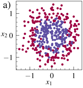
In order to demonstrate the behavior of the model described by the differential equation (56) it is convenient to consider data described by only two features and , because such data can be visualized as points in the Euclidean plane. We limit the number of classes to two and will consider a dataset shown in figure 2 a). The dataset consist samples of a Gaussian noise with standard deviation added to the two concentric circles where the outer circle has two times larger radius than the inner circle.
In the first model the differential equation (56) is solved on the space, giving the solutions , . According to [26], the dataset is hard to learn using such an equation, because the differential equation can only continuously deform the input space. Using the forward Euler method, described by the equation (109), we discretize the continuous variable into steps, producing a neural network with layers, each layer containing units. Softmax of the output of the final layer is calculated to get the predicted probabilities of the two classes. Similar to learnable parameter of nonlinearity in Parametric ReLUs [34], we consider the nonlinearity as an additional parameter to be learned. Thus the neural network has trainable parameters. Employing the regularization method described in section 3.5 we minimize the changes of the parameters between the neighboring layers and use the loss function
| (113) |
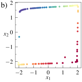
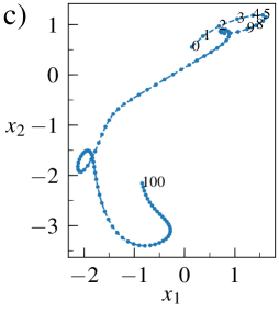
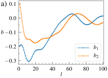
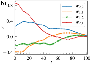
where is the usual cross entropy loss. We take the regularization parameter in the loss (113). All trainable parameters of the neural network are initialized to zero, as described in section 4.4, and optimized using the stochastic gradient descent. The parameters and of the trained model are shown in figure 3 a) and b), respectively. We see that indeed the loss (113) produces smooth variations of the parameters with the layer number . The nonlinearity parameter acquires the value . Since each layer of the network has two units, we can interpret all activations as points in the same plane. After training, the transformed data in the output of the network is shown in the figure 2 b). As one can see, the points from the inner circle are moved to the upper left part of the plane, the points from the outer circle are moved to the lower right part. Plotting activations of each layer in the same plane we can draw the gradual transformation of an input by the differential equation (56) as a trajectory. Sample trajectory is shown in the figure 2 c). The trajectory has several parts that look like rotations of the point in the - plane, consistent with the description in section 4.2. However, the trajectory is complicated, reflecting the difficulty to learn the dataset.
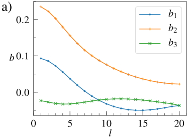
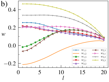
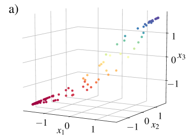
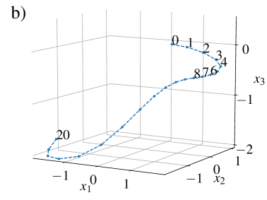
In the second model we solve the differential equation on the extended space, taking the initial condition . We discretize the continuous variable into steps, producing a neural network with layers, each layer containing units. The predicted probability of the first class is calculated as sigmoid of . We use loss (113) with the regularization parameter and fixed nonlinearity parameter . Consequently, the neural network has trainable parameters. The parameters and of the trained model are shown in figure 4 a) and b), respectively. After training, the transformed data in the output of the network is shown in the figure 5 a). As one can see, the points from the inner circle are moved to the upper part , the points from the outer circle are moved to the lower part . Sample trajectory, showing the gradual transformation of an input by the differential equation (56) is shown in the figure 5 b). We see that, compared with the first model, the trajectory is much simpler, indicating that the dataset is easier to learn using the second model. This fact that wider models are superior to thin and deep counterparts has been noticed for ResNets [43].
5.2 MNIST digit recognition
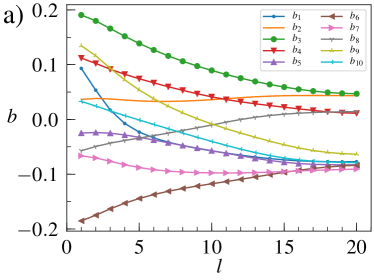
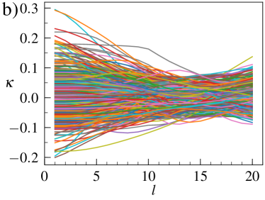
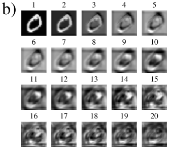
To demonstrate the behavior of the convolutional model described by the differential equation (75) we will consider recognition of digits from MNIST dataset. As is suggested in [26], we augment the solution space by adding new channels of zeros to the input image. We choose the number of additional channels equal to thus making the total number of channels equal to , which also is the number of classes. In the model we use convolutions with filter size. We discretize the continuous variable into steps, producing a neural network with convolutional layers. After the last convolutional layer we perform global max pooling and take softmax of the resulting numbers as the predicted probabilities of the classes. We consider the nonlinearity as an additional parameter to be learned. The resulting neural network has trainable parameters. As in previous subsection, we use the regularization method that minimize the changes of the parameters between the neighboring layers, taking the regularization parameter . All trainable parameters of the neural network are initialized to zero, as described in section 4.4, and optimized using the stochastic gradient descent. After training the network achieves 97.8% accuracy. The nonlinearity parameter acquires the value .
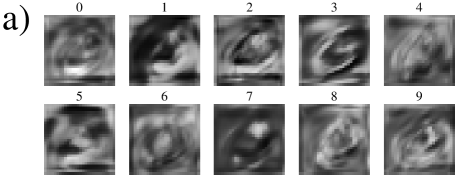
The parameters and of the trained model are shown in figure 6 a) and b), respectively. As in the previous subsection we see smooth variations of the parameters with the layer number . Sample activations of the final layer of the network when the initial image contains digit “0” are shown in the figure 7 a) and the corresponding activations in the first channel after each layer are shown in figure 7 b). As we can see in figure 7 b), the input image is gradually transformed by the neural network to the output activations.
6 Conclusions
To summarize, we investigated nonlinear differential equations (5) as machine learning models. The gradient of the loss function with respect to to the hidden state can be considered as a generalized momentum conjugate to the hidden state, and the differential equation for forward and backward propagation can be recast in Euler-Lagrange or Hamilton form. The corresponding Lagrangian and Hamiltonian are given by equations (19) and (21). The Euler-Lagrange and the Hamilton form of the equations allows analyze consequences of the possible symmetries in the models. Furthermore, we showed that not only residual networks, but also feedforward neural networks with small nonlinearities and the weights matrices deviating only slightly from identity matrices can be related to the differential equations. We proposed a differential equation (56) describing such networks.
References
- [1] Y. Bengio. Learning deep architectures for AI. Found. Trends Mach. Learn., 2(1):1–127, 2009.
- [2] Y. LeCun, Y. Bengio, and G. Hinton. Deep learning. Nature, 521:436, 2015.
- [3] S. Sonoda and N. Murata. Double continuum limit of deep neural networks. In ICML 2017 Workshop on Principled Approaches to Deep Learning, 2017.
- [4] S. Grossberg. Recurrent neural networks. Scholarpedia, 8(2):1888, 2013. revision #138057.
- [5] M. A. Cohen and S. Grossberg. Absolute stability of global pattern formation and parallel memory storage by competitive neural networks. IEEE Transactions on Systems, Man, and Cybernetics, SMC-13(5):815–826, 1983.
- [6] J. J. Hopfield. Neurons with graded response have collective computational properties like those of two-state neurons. Proc. Natl. Acad. Sci. USA, 81:3088–3092, 1984.
- [7] J. J. Hopfield. Hopfield network. Scholarpedia, 2(5):1977, 2007. revision #91363.
- [8] I. Harvey, P. Husbands, and D. Cliff. Seeing the light: Artificial evolution, real vision. In 3rd international conference on Simulation of adaptive behavior: from animals to animats, pages 392–401, 1994.
- [9] R. D. Beer. The dynamics of adaptive behavior: A research program. Robotics and Autonomous Systems, 20(2-4):257–289, 1997.
- [10] Matt Quinn. Evolving communication without dedicated communication channels. In Jozef Kelemen and Petr Sosík, editors, Advances in Artificial Life, pages 357–366. Springer, 2001.
- [11] K. He, X. Zhang, S. Ren, and J. Sun. Deep residual learning for image recognition. In 2016 IEEE Conference on Computer Vision and Pattern Recognition (CVPR), pages 770–778, June 2016.
- [12] Q. Liao and T. Poggio. Bridging the gaps between residual learning, recurrent neural networks and visual cortex. arXiv:1604.03640, 2016.
- [13] W. E. A proposal on machine learning via dynamical systems. Commun. Math. Stat., 5:1–11, 2017.
- [14] E. Haber, L. Ruthotto, E. Holtham, and S.-H. Jun. Learning across scales – multiscale methods for convolution neural networks. arXiv:1703:02009, 2017.
- [15] E. Haber and L. Ruthotto. Stable architectures for deep neural networks. Inverse Problems, 34:014004, 2018.
- [16] B. Chang, L. Meng, E. Haber, L. Ruthotto, D. Begert, and E. Holtham. Reversible architectures for arbitrarily deep residual neural networks. arXiv:1709.03698, 2017.
- [17] J. Behrmann, W. Grathwohl, R. T. Q. Chen, D. Duvenaud, and J.-H. Jacobsen. Invertible residual networks. arXiv:1811.00995, 2018.
- [18] Z. Li and Z. Shi. Deep residual learning and pdes on manifold. arXiv:1708.05115, 2017.
- [19] Y. Lu, A. Zhong, Q. Li, and B. Dong. Beyond finite layer neural networks: Bridging deep architectures and numerical differential equations. arXiv:1710:10121, 2017.
- [20] L. Ruthotto and E. Haber. Deep neural networks motivated by partial differential equations. arXiv:1804.04272, 2018.
- [21] Z. Long, Y. Lu, X. Ma, and B. Dong. PDE-Net: Learning PDEs from data. arXiv:1710.09668, 2017.
- [22] Z. Long, Y. Lu, and B. Dong. PDF-Net 2.0: Learning PDEs from data with a numeric-symbolic hybrid deep network. arXiv:1812:04426, 2018.
- [23] M. Y. Niu, I. L. Chuang, and L. Horesh. Recurrent neural networks in the eye of differential equations. arXiv:1904.12933, 2019.
- [24] T. Q. Chen, Y. Rubanova, J. Bettencourt, and D. K. Duvenaud. Neural ordinary differential equations. In S. Bengio, H. Wallach, H. Larochelle, K. Grauman, N. Cesa-Bianchi, and R. Garnett, editors, Advances in Neural Information Processing Systems 31, pages 6571–6583. Curran Associates, Inc., 2018.
- [25] Y. Rubanova, R. T. Q. Chen, and D. Duvenaud. Latent ODEs for irregularly-sampled time series. arXiv:1907.03907, 2019.
- [26] E. Dupont, A. Doucet, and Y. W. Teh. Augmented neural ODEs. arXiv:1904:01681, 2019.
- [27] L. S. Pontryagin, E. F. Mishchenko, V. G. Boltyanskii, and R. V. Gamkrelidze. The mathematical theory of optimal processes. Classics of Soviet mathematics. Routledge, Boca Raton, 4th ed edition, 2018.
- [28] M. Giaquinta and S. Hildebrandt. Calculus of variations I. Grundlehren der mathematischen Wissenschaften Vol 1. Springer, 2006.
- [29] D. E. Rumelhart, G. E. Hinton, and R. J. Williams. Learning representations by back-propagating errors. Nature, 323:533–536, 1986.
- [30] N. H. Ibragimov. Integrating factors, adjoint equations and lagrangians. J. Math. Anal. Appl., 318:742–757, 2006.
- [31] E. Noether. Invariante variationsprobleme. In Göttingen Math. Phys. Kl., pages 235–257. Königliche Gesellschaft der Wissenschaften, 1918. English transl.: Transport Theory and Statistical Physics 1(3): 186–207, 1971.
- [32] R. K. Srivastava, K. Greff, and J. Schmidhuber. Highway networks. arXiv:1505.00387, 2015.
- [33] R. K. Srivastava, K. Greff, and J. Schmidhuber. Training very deep networks. arXiv:1507.06228, 2015.
- [34] K. He, X. Zhang, S. Ren, and J. Sun. Delving deep into rectifiers: Surpassing human-level performance on imagenet classification. In 2015 IEEE International Conference on Computer Vision (ICCV), pages 1026–1034, Dec 2015.
- [35] G. E. Hinton, N. Srivastava, A. Krizhevsky, I. Sutskever, and R. R. Salakhutdinov. Improving neural networks by preventing co-adaptation of feature detectors. arXiv:1207.0580, 2012.
- [36] P. Y. Simard, D. Steinkraus, and J. Platt. Best practices for convolutional neural networks applied to visual document analysis. In Seventh International Conference on Document Analysis and Recognition, 2003. Proceedings., pages 958–963. Institute of Electrical and Electronics Engineers, Inc., August 2003.
- [37] G. Montavon, G. Orr, and K.-R. Müller, editors. Neural networks: tricks of the trade. Springer, 2012.
- [38] N. Morgan and H. Bourlard. Generalization and parameter estimation in feedforward nets: Some experiments. In D. S. Touretzky, editor, Advances in Neural Information Processing Systems 2, pages 630–637. Morgan Kaufmann Publishers Inc., San Francisco, CA, USA, 1990.
- [39] N. Srivastava, G. E. Hinton, A. Krizhevsky, I. Sutskever, and R. Salakhutdinov. Dropout: a simple way to prevent neural networks from overfitting. Journal of Machine Learning Research, 15(1):1929–1958, 2014.
- [40] X. Glorot and Y. Bengio. Understanding the difficulty of training deep feedforward neural networks. In Y. W. Teh and M. Titterington, editors, Proceedings of the Thirteenth International Conference on Artificial Intelligence and Statistics, volume 9 of Proceedings of Machine Learning Research, pages 249–256, Chia Laguna Resort, Sardinia, Italy, 13–15 May 2010. PMLR.
- [41] A. Krizhevsky, I. Sutskever, and G. E. Hinton. Imagenet classification with deep convolutional neural networks. In Proceedings of the 25th International Conference on Neural Information Processing Systems - Volume 1, NIPS’12, pages 1097–1105, USA, 2012. Curran Associates Inc.
- [42] J. C. Butcher. Numerical Methods for Ordinary Differential Equations. J. Wiley, 2003.
- [43] S. Zagoruyko and N. Komodakis. Wide residual networks. In BMVC, 2016.
Appendix A Alternative method of derivation of differential equation for backward propagation
Instead of variational calculus we can employ a simpler method by discretizing the equation (5) using a small time step as
| (A.1) |
with and taking the limit afterwards. This equation leads to the following Jacobian of the layer transform:
| (A.2) |
In order to calculate the gradients of a loss function with respect to the parameters of the network, one needs to have the gradients with respect to the activations of each layer. The gradient of the loss with respect to the activations of the -th layer is related to the gradient with respect to the activations of the -th layer via the equation
| (A.3) |
Inserting the Jacobian (A.2) we obtain
| (A.4) |
where for the brevity we introduced the notation
| (A.5) |
Interpreting as a continuous variable and taking the limit we get the differential equation (11) for the backward propagation.
The gradients of the loss function with respect to the parameters can be calculated using the equations
| (A.6) |
where the derivatives
| (A.7) |
are obtained from the equation (A.1). Equations (A.6), (A.7) lead to the gradients of the loss function
| (A.8) |
In the limit the gradients vanish. However, taking the learning rate proportional to , , one can get finite updates of the parameters in the gradient descent step. If the functions depend on parameters that do not depend on , , then the gradient of the loss can be calculated as
| (A.9) |
Using equation (A.8) and taking the limit we get equation (14).