Balancing Reconstruction Quality and Regularisation in Evidence Lower Bound for Variational Autoencoders

Abstract

A trade-off exists between reconstruction quality and the prior regularisation in the Evidence Lower Bound (ELBO) loss that Variational Autoencoder (VAE) models use for learning. There are few satisfactory approaches to deal with a balance between the prior and reconstruction objective, with most methods dealing with this problem through heuristics. In this paper, we show that the noise variance (often set as a fixed value) in the Gaussian likelihood $p({\mathbf{x}}|{\mathbf{z}})$ for real-valued data can naturally act to provide such a balance. By learning this noise variance so as to maximise the ELBO loss, we automatically obtain an optimal trade-off between the reconstruction error and the prior constraint on the posteriors. This variance can be interpreted intuitively as the necessary noise level for the current model to be the best explanation of the observed dataset. Further, by allowing the variance inference to be more flexible it can conveniently be used as an uncertainty estimator for reconstructed or generated samples. We demonstrate that optimising the noise variance is a crucial component of VAE learning, and showcase the performance on MNIST, Fashion MNIST and CelebA datasets. We find our approach can significantly improve the quality of generated samples whilst maintaining a smooth latent-space manifold to represent the data. The method also offers an indication of uncertainty in the final generative model.

1 Introduction

Variational Auto-encoders (VAEs, (?; ?)) are a stable and efficient approach to unsupervised learning. VAEs naturally combine two learning outcomes: enabling generation of data similar to the observations and secondly offering a probabilistic embedding scheme, in which the statistics at both sample and group levels satisfy required constraints. VAEs can, for example, be used for dimensionality reduction, feature extraction and efficient anomaly detection in the latent space.

Learning with a VAE naturally requires a balance between reconstruction loss minimisation and prior constraint enforcement. Several papers discuss the importance of this balance and the impact of different trade-off settings on the learned VAE models (?; ?). In (?), the authors propose scaling up the prior regularisation term in an attempt to promote disentanglement in the learnt representation. On the other hand, in (?) more emphasis is placed on the reconstruction loss term, to promote maximal information retention in the learned representation. The trade is most commonly adapted on a problem by problem basis (?; ?; ?).

In this paper, we propose a mechanism to optimise the trade-off between prior and reconstruction loss. We show that, by parameterising this balance via a variance parameter, we can achieve significant performance gains, both in terms of achieving a closer bound to the true data log likelihood as well as improving the generated sample quality. Unlike the hyperparameter introduced in (?), this variance hyperparameter intuitively represents the noise level in the dataset conditioned on the model explaining the observations. Furthermore, we develop a robust algorithm to learn to predict the variance hyperparameter conditioned on a given input. We show that the predicted variance can be used as an effective uncertainty estimator for reconstructed or generated samples.

By altering the strength of the prior regularisation term, the gap between the marginal latent distribution and the prior, measured for example using the Kullback Leibler (KL) divergence between the aggegate posterior and prior of the learnt model, becomes more prominent. This can significantly damage the quality of the generated samples as measured by common perceptual metrics such as the Inception Score (IS) (?) or the Frechet Inception Distance (FID) (?). To avoid this problem, we propose a simple approximation to the learned latent marginal distribution and use this approximate distribution, rather than the prior, to generate samples.

In summary, our contributions are:

• We show how optimisation of the variance hyperparameter under the VAE ELBO loss allows us to automate the trade-off between the reconstruction loss and the prior regularisation and we propose a stable learning procedure to accomplish this optimisation.

• We study the impact of sampling from the learned latent marginal distribution as opposed to the prior and propose to use an approximate marginal distribution instead of the prior to generate samples.

2 Background

2.1 VAE ELBO Loss

Given a dataset of $N$ observations $\mathcal{D}_{N}=\{{\bm{x}}_{1},{\bm{x}}_{2},\cdots,{\bm{x}}_{N}\}$ and a latent variable model $p_{\theta}({\mathbf{x}},{\mathbf{z}})=p_{\theta}({\mathbf{x}}|{\mathbf{z}})p({\mathbf{z}})$, the learning objective in VAEs maximises the marginal likelihood for all the data points in $\mathcal{D}_{N}$ under the model parameter $\theta$, i.e.

$$\operatorname*{arg\,max}_{\theta}\mathbb{E}_{p_{\mathcal{D}}({\mathbf{x}})}[\log p_{\theta}({\mathbf{x}})],$$ (1)

where $p_{\mathcal{D}}$ describes the true data distribution and $p_{\theta}({\mathbf{x}})=\int p_{\theta}({\mathbf{x}}|{\mathbf{z}})p({\mathbf{z}})\textrm{d}{\mathbf{z}}$ is the marginal distribution of ${\mathbf{x}}$ under the latent variable model by integrating out ${\mathbf{z}}$ according to a prior distribution $p({\mathbf{z}})$. Directly evaluating Equation (1) is often not feasible, because $p_{\theta}({\mathbf{x}}|{\mathbf{z}})$ is often parameterised by a neural network and integration over such a function cannot be easily evaluated. Instead, we can use variational evidence lower bound (ELBO) $\mathcal{L}({\mathbf{x}};\theta,\phi)$ on $\log p_{\theta}({\mathbf{x}})$ as an alternative objective by introducing an amortized inference model $q_{\phi}({\mathbf{z}}|{\mathbf{x}})$, as shown below:

$$\log p_{\theta}({\mathbf{x}})\geq\,\mathcal{L}({\mathbf{x}};\theta,\phi)$$ (2)

$$\mathrel{\ensurestackMath{\stackon[1pt]{=}{\scriptscriptstyle\Delta}}}\;\log\;p_{\theta}({\mathbf{x}})-D_{\mathrm{KL}}\big{[}\,q_{\phi}({\mathbf{z}}|{\mathbf{x}})\|p_{\theta}({\mathbf{z}}|{\mathbf{x}})$$

$$\mathrel{\ensurestackMath{\stackon[1pt]{=}{\scriptscriptstyle\Delta}}}\;\mathbb{E}_{q_{\phi}({\mathbf{z}}|{\mathbf{x}})}\big{[}\log p_{\theta}({\mathbf{x}}|{\mathbf{z}})\big{]}-D_{\mathrm{KL}}\big{[}\,q_{\phi}({\mathbf{z}}|{\mathbf{x}})\|p({\mathbf{z}})\big{]}.$$ (3)

Substituting $\mathcal{L}({\mathbf{x}};\theta,\phi)$ in (3) into the VAE objective (1) and evaluating the expectation wrt $p_{\mathcal{D}}$ with an empirical approximation, i.e. $p_{\mathcal{D}}({\mathbf{x}})\approx\frac{1}{N}\sum_{i=1}^{N}\delta({\bm{x}}_{i})$, we have the final VAE learning objective:

$$\frac{1}{N}\sum_{i=1}^{N}\Big{[}\underbrace{\mathbb{E}_{q_{\phi}({\mathbf{z}}|{\bm{x}}_{i})}\big{[}\log p_{\theta}({\bm{x}}_{i}|{\mathbf{z}})\big{]}}_{\text{ \leavevmode\hbox to11.75pt{\vbox to11.75pt{\pgfpicture\makeatletter\hbox{\hskip 5.87407pt\lower-5.87407pt\hbox to0.0pt{\pgfsys@beginscope\pgfsys@invoke{ }\definecolor{pgfstrokecolor}{rgb}{0,0,0}\pgfsys@color@rgb@stroke{0}{0}{0}\pgfsys@invoke{ }\pgfsys@color@rgb@fill{0}{0}{0}\pgfsys@invoke{ }\pgfsys@setlinewidth{0.4pt}\pgfsys@invoke{ }\nullfont\hbox to0.0pt{\pgfsys@beginscope\pgfsys@invoke{ }{ {{}}\hbox{\hbox{{\pgfsys@beginscope\pgfsys@invoke{ }{{}{{{}}}{{}}{}{}{}{}{}{}{}{}{}{{}\pgfsys@moveto{5.67407pt}{0.0pt}\pgfsys@curveto{5.67407pt}{3.13374pt}{3.13374pt}{5.67407pt}{0.0pt}{5.67407pt}\pgfsys@curveto{-3.13374pt}{5.67407pt}{-5.67407pt}{3.13374pt}{-5.67407pt}{0.0pt}\pgfsys@curveto{-5.67407pt}{-3.13374pt}{-3.13374pt}{-5.67407pt}{0.0pt}{-5.67407pt}\pgfsys@curveto{3.13374pt}{-5.67407pt}{5.67407pt}{-3.13374pt}{5.67407pt}{0.0pt}\pgfsys@closepath\pgfsys@moveto{0.0pt}{0.0pt}\pgfsys@stroke\pgfsys@invoke{ } }{{{{}}\pgfsys@beginscope\pgfsys@invoke{ }\pgfsys@transformcm{1.0}{0.0}{0.0}{1.0}{-1.75pt}{-2.25555pt}\pgfsys@invoke{ }\hbox{{\definecolor{pgfstrokecolor}{rgb}{0,0,0}\pgfsys@color@rgb@stroke{0}{0}{0}\pgfsys@invoke{ }\pgfsys@color@rgb@fill{0}{0}{0}\pgfsys@invoke{ }\hbox{{1}} }}\pgfsys@invoke{\lxSVG@closescope }\pgfsys@endscope}}} \pgfsys@invoke{\lxSVG@closescope }\pgfsys@endscope}}} } \pgfsys@invoke{\lxSVG@closescope }\pgfsys@endscope{{{}}}{}{}\hss}\pgfsys@discardpath\pgfsys@invoke{\lxSVG@closescope }\pgfsys@endscope\hss}}\lxSVG@closescope\endpgfpicture}} {Reconstruction likelihood}}}-\underbrace{D_{\mathrm{KL}}\big{[}\,q_{\phi}({\mathbf{z}}|{\bm{x}}_{i})\,\|\,p({\mathbf{z}})\big{]}}_{\text{ \leavevmode\hbox to11.75pt{\vbox to11.75pt{\pgfpicture\makeatletter\hbox{\hskip 5.87407pt\lower-5.87407pt\hbox to0.0pt{\pgfsys@beginscope\pgfsys@invoke{ }\definecolor{pgfstrokecolor}{rgb}{0,0,0}\pgfsys@color@rgb@stroke{0}{0}{0}\pgfsys@invoke{ }\pgfsys@color@rgb@fill{0}{0}{0}\pgfsys@invoke{ }\pgfsys@setlinewidth{0.4pt}\pgfsys@invoke{ }\nullfont\hbox to0.0pt{\pgfsys@beginscope\pgfsys@invoke{ }{ {{}}\hbox{\hbox{{\pgfsys@beginscope\pgfsys@invoke{ }{{}{{{}}}{{}}{}{}{}{}{}{}{}{}{}{{}\pgfsys@moveto{5.67407pt}{0.0pt}\pgfsys@curveto{5.67407pt}{3.13374pt}{3.13374pt}{5.67407pt}{0.0pt}{5.67407pt}\pgfsys@curveto{-3.13374pt}{5.67407pt}{-5.67407pt}{3.13374pt}{-5.67407pt}{0.0pt}\pgfsys@curveto{-5.67407pt}{-3.13374pt}{-3.13374pt}{-5.67407pt}{0.0pt}{-5.67407pt}\pgfsys@curveto{3.13374pt}{-5.67407pt}{5.67407pt}{-3.13374pt}{5.67407pt}{0.0pt}\pgfsys@closepath\pgfsys@moveto{0.0pt}{0.0pt}\pgfsys@stroke\pgfsys@invoke{ } }{{{{}}\pgfsys@beginscope\pgfsys@invoke{ }\pgfsys@transformcm{1.0}{0.0}{0.0}{1.0}{-1.75pt}{-2.25555pt}\pgfsys@invoke{ }\hbox{{\definecolor{pgfstrokecolor}{rgb}{0,0,0}\pgfsys@color@rgb@stroke{0}{0}{0}\pgfsys@invoke{ }\pgfsys@color@rgb@fill{0}{0}{0}\pgfsys@invoke{ }\hbox{{2}} }}\pgfsys@invoke{\lxSVG@closescope }\pgfsys@endscope}}} \pgfsys@invoke{\lxSVG@closescope }\pgfsys@endscope}}} } \pgfsys@invoke{\lxSVG@closescope }\pgfsys@endscope{{{}}}{}{}\hss}\pgfsys@discardpath\pgfsys@invoke{\lxSVG@closescope }\pgfsys@endscope\hss}}\lxSVG@closescope\endpgfpicture}} {Prior constraint}}}\Big{]}.$$ (4)

Facilitated with the reparameterisation trick (?), the above ELBO loss can be optimised with stochastic gradient descent algorithms, leading to an efficient learning method (?; ?).

2.2 Competing Learning Objectives in ELBO

The two terms in the ELBO loss (Eq. 4) control different behaviours of the model. The reconstruction likelihood term attempts to reconstruct the input ${\bm{x}}_{i}$ as faithfully as possible. The prior constraint term enforces the posterior distribution of ${\bm{x}}_{i}$ under the encoding function to comply with an assumed prior $p({\mathbf{z}})$ and if the constraint is effectively imposed, the aggregate posterior of the entire dataset (?) is likely to be very close to the prior, indicating the data distribution has been successfully projected to the target prior in the latent space. Optimizing the two losses together, we would hope to simultaneously achieve the best performance in both terms.

Unfortunately, the two losses are often conflicting. To see this, consider if is maximized, then the embeddings of different input samples ${\bm{x}}_{i}$ and ${\bm{x}}_{j}$ can be easily distinguished, i.e. $D_{\mathrm{KL}}\big{[}q_{\phi}({\mathbf{z}}|{\bm{x}}_{i})\,\|\,q_{\phi}({\mathbf{z}}|{\bm{x}}_{j})\big{]}$ should be large. On the other hand, if is satisfied, then all sample embeddings should approach $q({\mathbf{z}})$, i.e. $D_{\mathrm{KL}}\big{[}q_{\phi}({\mathbf{z}}|{\bm{x}}_{i})\,\|\,q_{\phi}({\mathbf{z}}|{\bm{x}}_{j})\big{]}$ should be zero. Therefore, and almost always influence each other. As a result, finding the optimal balance between the two terms is a crucial part in the VAE learning process. Unfortunately, there has not been a satisfying solution and most methods handle this problem by introducing weight hyperparameters on the two losses and choose their values based on heuristics (?; ?; ?).

3 Our Proposal

In this work, we propose a method that automatically finds the best balance between the two contradicting objectives in the VAE ELBO loss.

3.1 Gaussian Likelihood in the Generative Model

For real-valued data ${\mathbf{x}}$, we can use a Gaussian distribution to model the conditional distribution $p_{\theta}({\bm{x}}_{i}|{\mathbf{z}})$ in the generative model, i.e.

$$p_{\theta}({\bm{x}}_{i}^{k}|{\mathbf{z}})=\frac{1}{{(2\pi)}^{\frac{1}{2}}\sigma}\exp{\Bigg{(}-\frac{\big{(}g_{\theta}^{k}({\mathbf{z}})-{\bm{x}}_{i}^{k}\big{)}^{2}}{2\sigma^{2}}\Bigg{)}},$$ (5)

where $\sigma^{2}$ is a common global variance parameter, reflecting the global noise properties of the data; $g_{\theta}(\cdot)$ represents a nonlinear mapping that transforms an encoding ${\mathbf{z}}$ in the latent space to the data space; and $k$ represents the $k$-th dimension of the data variable ${\mathbf{x}}$. If we assume that different dimensions in ${\mathbf{x}}$ are independent, then the conditional density of the complete data variable is

$$p_{\theta}({\bm{x}}_{i}|{\mathbf{z}})=\prod_{k=1}^{d}p_{\theta}({\bm{x}}_{i}^{k}|{\mathbf{z}}),$$ (6)

where $d$ is the dimension of the data variable ${\mathbf{x}}$. Therefore, $\log p_{\theta}({\bm{x}}_{i}|{\mathbf{z}})$ in the ELBO loss given by (4) can be computed as

$$\log p_{\theta}({\bm{x}}_{i}|{\mathbf{z}})=-\frac{d}{2}\log(2\pi)-d\log\sigma-\frac{1}{2\sigma^{2}}\sum_{k=1}^{d}\big{(}g_{\theta}^{k}({\mathbf{z}})-{\bm{x}}_{i}^{k}\big{)}^{2}.$$ (7)

Notice the terms inside the summation are element-wise square errors between the generated sample and the original sample and $\frac{1}{2\sigma^{2}}$ naturally appears as a weighting factor on the sum of square error term. When $\log p_{\theta}({\bm{x}}_{i}|{\mathbf{z}})$ is maximised, the $\log\sigma$ term has an important regularizing effect on the $\sigma$ value: it prevents $\sigma$ from taking very large values, which would allow the generator function $g(\cdot)$ to produce arbitrarily bad reconstruction.

3.2 ELBO Loss with A Global Variance Parameter

Substituting (7) into (4), we have the overall ELBO loss with the Gaussian likelihood assumption as

$$\begin{split}&\mathbb{E}_{p_{\mathcal{D}}({\mathbf{x}})}[\log p_{\theta}({\mathbf{x}})]\geq-\frac{1}{N}\sum_{i=1}^{N}\Bigg{[}\frac{d}{2}\log(2\pi)+d\log\sigma+\\ &\underbrace{\frac{1}{2\sigma^{2}}}_{\text{ \leavevmode\hbox to11.75pt{\vbox to11.75pt{\pgfpicture\makeatletter\hbox{\hskip 5.87407pt\lower-5.87407pt\hbox to0.0pt{\pgfsys@beginscope\pgfsys@invoke{ }\definecolor{pgfstrokecolor}{rgb}{0,0,0}\pgfsys@color@rgb@stroke{0}{0}{0}\pgfsys@invoke{ }\pgfsys@color@rgb@fill{0}{0}{0}\pgfsys@invoke{ }\pgfsys@setlinewidth{0.4pt}\pgfsys@invoke{ }\nullfont\hbox to0.0pt{\pgfsys@beginscope\pgfsys@invoke{ }{ {{}}\hbox{\hbox{{\pgfsys@beginscope\pgfsys@invoke{ }{{}{{{}}}{{}}{}{}{}{}{}{}{}{}{}{{}\pgfsys@moveto{5.67407pt}{0.0pt}\pgfsys@curveto{5.67407pt}{3.13374pt}{3.13374pt}{5.67407pt}{0.0pt}{5.67407pt}\pgfsys@curveto{-3.13374pt}{5.67407pt}{-5.67407pt}{3.13374pt}{-5.67407pt}{0.0pt}\pgfsys@curveto{-5.67407pt}{-3.13374pt}{-3.13374pt}{-5.67407pt}{0.0pt}{-5.67407pt}\pgfsys@curveto{3.13374pt}{-5.67407pt}{5.67407pt}{-3.13374pt}{5.67407pt}{0.0pt}\pgfsys@closepath\pgfsys@moveto{0.0pt}{0.0pt}\pgfsys@stroke\pgfsys@invoke{ } }{{{{}}\pgfsys@beginscope\pgfsys@invoke{ }\pgfsys@transformcm{1.0}{0.0}{0.0}{1.0}{-1.75pt}{-2.25555pt}\pgfsys@invoke{ }\hbox{{\definecolor{pgfstrokecolor}{rgb}{0,0,0}\pgfsys@color@rgb@stroke{0}{0}{0}\pgfsys@invoke{ }\pgfsys@color@rgb@fill{0}{0}{0}\pgfsys@invoke{ }\hbox{{3}} }}\pgfsys@invoke{\lxSVG@closescope }\pgfsys@endscope}}} \pgfsys@invoke{\lxSVG@closescope }\pgfsys@endscope}}} } \pgfsys@invoke{\lxSVG@closescope }\pgfsys@endscope{{{}}}{}{}\hss}\pgfsys@discardpath\pgfsys@invoke{\lxSVG@closescope }\pgfsys@endscope\hss}}\lxSVG@closescope\endpgfpicture}}}}\mathbb{E}_{q_{\phi}({\mathbf{z}}|{\bm{x}}_{i})}\bigg{[}\underbrace{\sum_{k=1}^{d}\big{(}g_{\theta}^{k}({\mathbf{z}})-{\bm{x}}_{i}^{k}\big{)}^{2}}_{\text{ \leavevmode\hbox to11.75pt{\vbox to11.75pt{\pgfpicture\makeatletter\hbox{\hskip 5.87407pt\lower-5.87407pt\hbox to0.0pt{\pgfsys@beginscope\pgfsys@invoke{ }\definecolor{pgfstrokecolor}{rgb}{0,0,0}\pgfsys@color@rgb@stroke{0}{0}{0}\pgfsys@invoke{ }\pgfsys@color@rgb@fill{0}{0}{0}\pgfsys@invoke{ }\pgfsys@setlinewidth{0.4pt}\pgfsys@invoke{ }\nullfont\hbox to0.0pt{\pgfsys@beginscope\pgfsys@invoke{ }{ {{}}\hbox{\hbox{{\pgfsys@beginscope\pgfsys@invoke{ }{{}{{{}}}{{}}{}{}{}{}{}{}{}{}{}{{}\pgfsys@moveto{5.67407pt}{0.0pt}\pgfsys@curveto{5.67407pt}{3.13374pt}{3.13374pt}{5.67407pt}{0.0pt}{5.67407pt}\pgfsys@curveto{-3.13374pt}{5.67407pt}{-5.67407pt}{3.13374pt}{-5.67407pt}{0.0pt}\pgfsys@curveto{-5.67407pt}{-3.13374pt}{-3.13374pt}{-5.67407pt}{0.0pt}{-5.67407pt}\pgfsys@curveto{3.13374pt}{-5.67407pt}{5.67407pt}{-3.13374pt}{5.67407pt}{0.0pt}\pgfsys@closepath\pgfsys@moveto{0.0pt}{0.0pt}\pgfsys@stroke\pgfsys@invoke{ } }{{{{}}\pgfsys@beginscope\pgfsys@invoke{ }\pgfsys@transformcm{1.0}{0.0}{0.0}{1.0}{-1.75pt}{-2.25555pt}\pgfsys@invoke{ }\hbox{{\definecolor{pgfstrokecolor}{rgb}{0,0,0}\pgfsys@color@rgb@stroke{0}{0}{0}\pgfsys@invoke{ }\pgfsys@color@rgb@fill{0}{0}{0}\pgfsys@invoke{ }\hbox{{1}} }}\pgfsys@invoke{\lxSVG@closescope }\pgfsys@endscope}}} \pgfsys@invoke{\lxSVG@closescope }\pgfsys@endscope}}} } \pgfsys@invoke{\lxSVG@closescope }\pgfsys@endscope{{{}}}{}{}\hss}\pgfsys@discardpath\pgfsys@invoke{\lxSVG@closescope }\pgfsys@endscope\hss}}\lxSVG@closescope\endpgfpicture}}}}\bigg{]}+\underbrace{D_{\mathrm{KL}}\Big{[}\,q_{\phi}({\mathbf{z}}|{\bm{x}}_{i})\,\|\,p({\mathbf{z}})\Big{]}}_{\text{ \leavevmode\hbox to11.75pt{\vbox to11.75pt{\pgfpicture\makeatletter\hbox{\hskip 5.87407pt\lower-5.87407pt\hbox to0.0pt{\pgfsys@beginscope\pgfsys@invoke{ }\definecolor{pgfstrokecolor}{rgb}{0,0,0}\pgfsys@color@rgb@stroke{0}{0}{0}\pgfsys@invoke{ }\pgfsys@color@rgb@fill{0}{0}{0}\pgfsys@invoke{ }\pgfsys@setlinewidth{0.4pt}\pgfsys@invoke{ }\nullfont\hbox to0.0pt{\pgfsys@beginscope\pgfsys@invoke{ }{ {{}}\hbox{\hbox{{\pgfsys@beginscope\pgfsys@invoke{ }{{}{{{}}}{{}}{}{}{}{}{}{}{}{}{}{{}\pgfsys@moveto{5.67407pt}{0.0pt}\pgfsys@curveto{5.67407pt}{3.13374pt}{3.13374pt}{5.67407pt}{0.0pt}{5.67407pt}\pgfsys@curveto{-3.13374pt}{5.67407pt}{-5.67407pt}{3.13374pt}{-5.67407pt}{0.0pt}\pgfsys@curveto{-5.67407pt}{-3.13374pt}{-3.13374pt}{-5.67407pt}{0.0pt}{-5.67407pt}\pgfsys@curveto{3.13374pt}{-5.67407pt}{5.67407pt}{-3.13374pt}{5.67407pt}{0.0pt}\pgfsys@closepath\pgfsys@moveto{0.0pt}{0.0pt}\pgfsys@stroke\pgfsys@invoke{ } }{{{{}}\pgfsys@beginscope\pgfsys@invoke{ }\pgfsys@transformcm{1.0}{0.0}{0.0}{1.0}{-1.75pt}{-2.25555pt}\pgfsys@invoke{ }\hbox{{\definecolor{pgfstrokecolor}{rgb}{0,0,0}\pgfsys@color@rgb@stroke{0}{0}{0}\pgfsys@invoke{ }\pgfsys@color@rgb@fill{0}{0}{0}\pgfsys@invoke{ }\hbox{{2}} }}\pgfsys@invoke{\lxSVG@closescope }\pgfsys@endscope}}} \pgfsys@invoke{\lxSVG@closescope }\pgfsys@endscope}}} } \pgfsys@invoke{\lxSVG@closescope }\pgfsys@endscope{{{}}}{}{}\hss}\pgfsys@discardpath\pgfsys@invoke{\lxSVG@closescope }\pgfsys@endscope\hss}}\lxSVG@closescope\endpgfpicture}}}}\Bigg{]}.\end{split}$$ (8)

From Equation (8), we can see that term represents a relative weighting $\frac{1}{2\sigma^{2}}$ between the two competing learning objectives; the reconstruction error; and prior constraint on the posteriors $q_{\phi}({\mathbf{z}}|{\bm{x}}_{i})$. If we optimise the ELBO in (8) w.r.t. $\theta$, $\phi$ and $\sigma$, then we will reach a maximised lower bound of the data likelihood where the model automatically balances between the objectives of minimizing the information loss through the auto-encoding process while still having the latent marginal distribution remain close to the prior distribution. The optimal $\sigma^{2}$, which is obtained at the maximal ELBO and denoted as $\sigma_{*}^{2}$, can be interpreted as the amount of noise that has to be assumed in the dataset for the current reconstruction to be considered as the best explanation of the observed samples.

3.3 Closed-form Solution for the Variance

For fixed $\theta$ and $\phi$, we can derive a closed form solution for the optimal global variance $\sigma_{*}^{2}$. To compute $\sigma_{*}^{2}$, we take derivative of $\mathbb{E}_{p_{\mathcal{D}}({\mathbf{x}})}[\log p_{\theta}({\mathbf{x}})]$ in Equation (8) wrt $\sigma$ and set it to zero. Then

$${\sigma_{*}}^{2}=\frac{1}{d}\mathbb{E}_{q_{\phi}({\mathbf{z}}|{\bm{x}}_{i})}\bigg{[}\sum_{k=1}^{d}\big{(}g_{\theta}^{k}({\mathbf{z}})-{\bm{x}}_{i}^{k}\big{)}^{2}\bigg{]}.$$ (9)

The significance of this result is that it improves the stability of the learning process with the additional $\sigma^{2}$ parameter, as we can always find a local minimum of the ELBO loss by updating $\sigma^{2}$ and the model parameters $\theta$ and $\phi$ iteratively.

3.4 More Flexible Variance Estimation

So far we have taken $\sigma^{2}$ to be the same value for the entire dataset and across all data dimensions, but nothing stops us here. We can extend the $\sigma^{2}$ estimation to be conditioned on particular encodings, be that an encoding of a real data sample or a sampled latent code from the prior distribution. We can also allow $\sigma^{2}$ to differ across data dimensions and such $\sigma^{2}$ can conveniently highlights the regions with high uncertainty in a reconstructed or generated sample. To achieve these goals, we need to replace the global variance $\sigma^{2}$ in Equation (5) by a variance estimation function $\sigma_{\theta}^{k}({\mathbf{z}})$ which is parameterised by $\theta$ and conditioned on data dimension $k$ and an input encoding ${\mathbf{z}}$. The corresponding $\log p_{\theta}({\bm{x}}_{i}|{\mathbf{z}})$ now becomes

$$-\frac{d}{2}\log(2\pi)-\sum_{k=1}^{d}\bigg{[}\frac{1}{2\big{(}\sigma_{\theta}^{k}({\mathbf{z}})\big{)}^{2}}\big{(}g_{\theta}^{k}({\mathbf{z}})-{\bm{x}}_{i}^{k}\big{)}^{2}+\log\sigma_{\theta}^{k}({\mathbf{z}})\bigg{]}.$$ (10)

Substituting (10) in (4), we get the ELBO loss associated with the input dependent variance estimation and learning can be done by optimising this ELBO wrt to all model parameters $\theta$ and $\phi$.

However, we notice that learning to predict $\sigma_{\theta}^{k}({\mathbf{z}})$ together with learning the parameters for the auto-encoding task from scratch turns out to be extremely challenging and the optimisation often gets stuck at predicting very small variance values. This is because the variance prediction is highly dependent on the reconstruction error given by the current model. At early stage when both the encoder and decoder are inaccurate, the reconstruction error is large and has high variance. This causes random updates in the variance prediction module. If the variance happens to arrive at a small value where the gradient of the $\log\sigma_{\theta}^{k}({\mathbf{z}})$ term dominates, then it is very hard for the gradient update to escape the strong negative gradient from the $\log$ function. To prevent this happening and obtain stable learning, we propose a staged learning process where we start with learning the global variance parameter until certain condition of convergence is reached and then we switch to the input dependent variance prediction module with the model parameters ($\phi$ and $\theta$) continuing updates from the optimised values given by the previous stage. We also use the optimised global variance as an effective lower bound to prevent the predicted variance from getting stuck at small values. The learning procedure is summarised in Algorithm 1.

3.5 Importance of Aggregate Posterior

Even when optimising the variance hyperparameter, the learnt posteriors might be quite different from the assumed prior distribution. If this is the case, then using the prior distribution to generate samples may no longer be a good idea. A better alternative is to generate samples from the aggregate posterior $q_{\phi}({\mathbf{z}})$, which can be considered as the data distribution in the latent space, defined (?) as

$$q_{\phi}({\mathbf{z}})=\mathbb{E}_{p_{\mathcal{D}}({\mathbf{x}})}[q_{\phi}({\mathbf{z}}|{\mathbf{x}})]\approx\frac{1}{N}\sum_{i=1}^{N}q_{\phi}({\mathbf{z}}|{\bm{x}}_{i}).$$ (11)

The approximation in (11) is made by evaluating the expectation w.r.t $p_{\mathcal{D}}({\mathbf{x}})$ empirically for $\mathcal{D}_{N}$ and with the isotropic Gaussian assumption for posteriors $q_{\phi}({\mathbf{z}}|{\mathbf{x}})$, the aggregate posterior is effectively a mixture of Gaussian distribution with $N$ mixture components. However, there are two problem with generating data samples directly from the aggregate posterior: 1) large memory is needed to store the statistics of all $N$ components in the aggregate posterior distribution and 2) as training data is finite, the aggregate posterior is likely to be overfitted to the training samples, which means that only samples very similar to the observed data will be generated.

We propose to address both problems by using a simpler approximate distribution to the true aggregate posterior. There are many choices for the approximate distribution. In our case, we simply use a Gaussian mixture distribution $\hat{q}({\mathbf{z}})$ with $M$ components ($M\ll N$ and we often take $M$=30 for simple datasets, such as MNIST and Fashion MNIST), as shown below:

$$q_{\phi}({\mathbf{z}})\approx\hat{q}({\mathbf{z}})=\sum_{m=1}^{M}w_{m}\mathcal{N}({\mathbf{z}};\mu_{m},\Sigma_{m}),$$ (12)

where $w_{m}$ is the weight for each Gaussian mixture ($w_{m}>0$ and $\sum_{m}w_{m}=1$) and $\mu_{m}$ and $\Sigma_{m}$ are the mean and covariance matrix for the $m$-th Gaussian mixture. The Gaussian mixture distribution is a good choice for the following reasons: 1) it is sufficiently expressive to represent the major modes and the low density regions that $q_{\phi}({\mathbf{z}})$ might possess; 2) with limited number of components, it is much simpler than the original aggregate posterior, significantly reducing the risk of overfitting; and 3) there are efficient algorithms, such as EM (?) and Variational Bayesian inference methods (?), to derive the Gaussian mixture approximation.

Algorithm 1 VAE learning with variance prediction

  $\phi$, $\theta$ $\leftarrow$ Initialize parameters

  $\sigma$ $\leftarrow$ Initialize as 1

  $\epsilon_{1}$, $\epsilon_{2}$, n_epoch_1, n_epoch_2 $\leftarrow$ Set stopping condition

  Set epoch counter $e=0$

  while e $<$ n_epoch_1 or $\delta_{\text{ELBO}}<\epsilon_{1}$ do

     Update $\phi$, $\theta$ and $\sigma$ using AdamOptimizer on the ELBO loss defined in Equation (8)

     $\delta_{\text{ELBO}}=\textrm{ELBO}_{e}-\textrm{ELBO}_{e-1}$

     e = e + 1

  end while

  while e $<$ n_epoch_2 or $\delta_{\text{ELBO}}<\epsilon_{2}$ do

     Freeze $\sigma^{2}$ value as $\sigma_{\textrm{dataset}}^{2}$

     Add the input dependent variance module with $\big{(}\sigma_{\theta}^{k}({\mathbf{z}})\big{)}^{2}=v_{\theta}^{k}({\mathbf{z}})+\frac{1}{2}\sigma_{\textrm{dataset}}^{2}$,

     Update $\phi$, $\theta$ using AdamOptimizer on the ELBO loss with the $\log p_{\theta}({\bm{x}}_{i}|{\mathbf{z}})$ term given by Equation (10).

     $\delta_{\text{ELBO}}=\textrm{ELBO}_{e}-\textrm{ELBO}_{e-1}$

     e = e + 1

  end while

  return $\phi,\theta,\sigma_{\textrm{dataset}}^{2}$

4 Related Work

Optimising the variance parameter in a likelihood model has been adopted in Mixture Density Networks (?) and Gaussian process regression models (?). Both works aim to learn a model for a regression task and use an isotropic Gaussian likelihood to model the conditional distribution $p({\mathbf{y}}|{\mathbf{x}})$ between an input ${\mathbf{x}}$ and an output ${\mathbf{y}}$. Although the nature of their learning tasks is vastly different from ours (supervised vs unsupervised), they emphasise the same message as our proposal that learning the variance parameter in the likelihood model for noisy observations is an integral part of the learning process and should not be omitted. Two major differences between our proposal and their treatment to the variance parameter are: 1) we extend the variance prediction to more flexible settings, such as being conditioned on an encoding and variable across data dimensions, whereas they only use a single-valued variance parameter; 2) the learning objective in their models only contains the Gaussian likelihood term and therefore they do not have the tradeoff between reconstruction and regularisation that we are faced with when using the ELBO loss. In the original VAE paper (?), estimation of a similar variance in the decoder is briefly mentioned in the appendix, where their decoder estimates a single-valued variance for a given input sample. However, such prediction is often unstable and thus our proposal uses a two-stage training procedure to stabilise the training.

The undesirable gap between the aggregate posterior and prior has been noted in (?). Many works have been proposed to mitigate such a gap by using either a more expressive model for sample posteriors $q_{\phi}({\mathbf{z}}|{\bm{x}}_{i})$ (?; ?; ?; ?) or a more flexible model for the prior $p(z)$ (?; ?). Our treatment of the gap differs from all the aforementioned works, as we realise that such gap is hard to be eliminated. Hence, the best remedy is to replace the prior with a distribution $\hat{p}({\mathbf{z}})$ that is better matched with the amortized posterior $q_{\phi}({\mathbf{z}}|{\mathbf{x}})$ and the generative likelihood $p_{\theta}({\mathbf{x}}|{\mathbf{z}})$ so that the gap between the amortized posterior $q_{\phi}({\mathbf{z}}|{\mathbf{x}})$ and the true posterior from the generative model $p_{\theta}({\mathbf{z}}|{\mathbf{x}})=\frac{p_{\theta}({\mathbf{x}}|{\mathbf{z}})\hat{p}({\mathbf{z}})}{\int p_{\theta}({\mathbf{x}}|{\mathbf{z}})\hat{p}({\mathbf{z}})\textrm{d}{\mathbf{z}}}$ can be effectively reduced, giving a closer bound to $\log p({\mathbf{x}})$.

5 Experiment Results

Table 1: Comparison of the aggregate posterior and its Gaussian mixture approximation (32 mixtures) for models learnt under different $\sigma^{2}$ values for MNIST dataset. $D_{\mathrm{KL}}(\hat{q}({\mathbf{z}})||p({\mathbf{z}}))$ denotes the gap between the approximate aggregate posterior and the prior distribution and is evaluated by Monte Carlo estimation of 10k samples (10 runs).

$\sigma^{2}$	1	0.5	0.035 (Optimal)	0.01	Prior
Aggregate posterior
Approximate aggregate posterior
[.5]0$D_{\mathrm{KL}}(\hat{q}({\mathbf{z}})||p({\mathbf{z}}))$	0.094 $\pm$ 0.003	0.132 $\pm$ 0.003	0.422 $\pm$ 0.011	1.552 $\pm$ 0.034

We carry out extensive experiments on MNIST (?), Fashion MNIST (?) and CelebA (?) datasets. For all datasets, we take the images as real-valued data so that our Gaussian likelihood assumption is appropriate. We take the original VAE and $\beta$-VAE as baseline methods for comparison. We also compare to WAE (?) and DIP-VAE (?) to demonstrate the significant performance gain given by optimising the variance parameter and sampling from the approximate aggregate posterior. More results and details of data pre-processing and model architectures are given in Supplemental Materials.

5.1 Intuition through visualisation

First we try to gain an intuitive understanding of the impact of learning the $\sigma^{2}$ parameter in our proposal. To this end, we trained VAE models of two dimensional latent space on MNIST dataset under different $\sigma^{2}$ values and in Table 1 we show log density plots of various distributions in the latent space.

When $\sigma^{2}$= 0.5, the weighting $\frac{1}{2\sigma^{2}}$ between the reconstruction loss and the prior constraint is equal and this corresponds to the original VAE learning objective. When $\sigma^{2}=1$, the weight on the reconstruction loss is halved, resulting in an increased penalty on the prior regularisation, and this leads to the $\beta$-VAE’s objective. $\sigma^{2}$= 0.035 is learnt under our proposal by optimising the ELBO in (8), which learns the optimal balance between the two losses. Finally, $\sigma^{2}$= 0.01 indicates the scenario where extreme penalty on the reconstruction loss is imposed.

From the visualisation, we can see that learning under different $\sigma^{2}$ values leads to very different inference models. Larger $\sigma^{2}$ values result in an aggregate posterior closer to the prior distribution and often corresponding to a smooth density. As the $\sigma^{2}$ gets smaller, sample posteriors become more distinctive and the aggregate posterior clearly becomes more complex and contains more sophisticated low density regions. Either end of the $\sigma^{2}$ value spectrum is sub-optimal: too large $\sigma^{2}$ causes severe information loss of the input data and too small $\sigma^{2}$ leads to a marginal distribution that is overly complex. We argue that the optimised $\sigma^{2}$ offers the best balance. More experimental evidence for this claim is given in Section 5.2.

(a) Optimised ELBO (higher is better).

(b) FID score (lower is better).

(c) $D_{\mathrm{KL}}(\hat{q}({\mathbf{z}})||p({\mathbf{z}}))$ (lower is better).

Figure 1: Impact of learning $\sigma^{2}$ on 3 metrics for VAE performance on MNIST dataset. Optimising $\sigma^{2}$ (green star) reaches the highest ELBO, very low in FID score and reasonably small $D_{\mathrm{KL}}(\hat{q}({\mathbf{z}})||p({\mathbf{z}}))$.

Table 2: FID scores compared across 5 different methods for MNIST, fashion MNIST and CelebA datasets. For all datasets, optimising $\sigma^{2}$ achieves the best visual quality (sample are generated from approx. aggregate posterior where possible).

[.5]0	Ours (optimising $\sigma^{2}$)	VAE (?)	$\beta$-VAE (?)	DIP-VAE (?)	WAE (?)	Real images
MNIST	8.9	74.9	438.1	114.9	142.8	1.9
Fashion MNIST	10.6	123.8	281.5	103.6	149.5	0.7
CelebA	74.7	78.4	106.4	87.5	85.4	2.9

Table 3: IWAE test log likelihood (LL, higher is better) for MNIST and Fashion MNIST compared across 4 different methods. In our proposal, we evaluate the LL for two different variance estimation settings: 1) a global variance of the entire dataset and 2) input dependent pixel level variances.

		Optimising $\sigma^{2}$ (Ours)		VAE	$\beta$-VAE	DIP-VAE
		dataset	pixel
MNIST	Prior	1307	6037	-462	-730	-461
	Approx. Agg. Posterior	1323	6052	-461	-730	-460
Fashion MNIST	Prior	1145	5708	-463	-731	-463
	Approx. Agg. Posterior	1157	5724	-462	-731	-462

The visualisation also demonstrates that except for extremely small $\sigma^{2}$ values, the Gaussian mixture model can effectively approximate the aggregate posterior. Thanks to the closed-form solution of the global variance parameter derived in (9) and the stabilised learning procedure introduced in Section 3.4, we will never enter these small $\sigma^{2}$ values regime in our learning scheme. Furthermore, the gap between the aggregate posterior and the prior persistently exists no matter what value $\sigma^{2}$ takes. There are good texts explaining why such a gap appears (?). We would like to stress that if such a gap is hard to avoid, then samples should not be naively generated from the prior distribution but from an alternative distribution that better represents the aggregate posterior. We delegate Section 5.3 for more detailed discussion on this gap.

5.2 Performance Gain from Optimizing $\sigma^{2}$

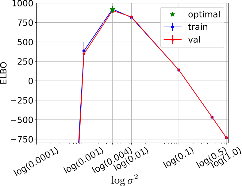
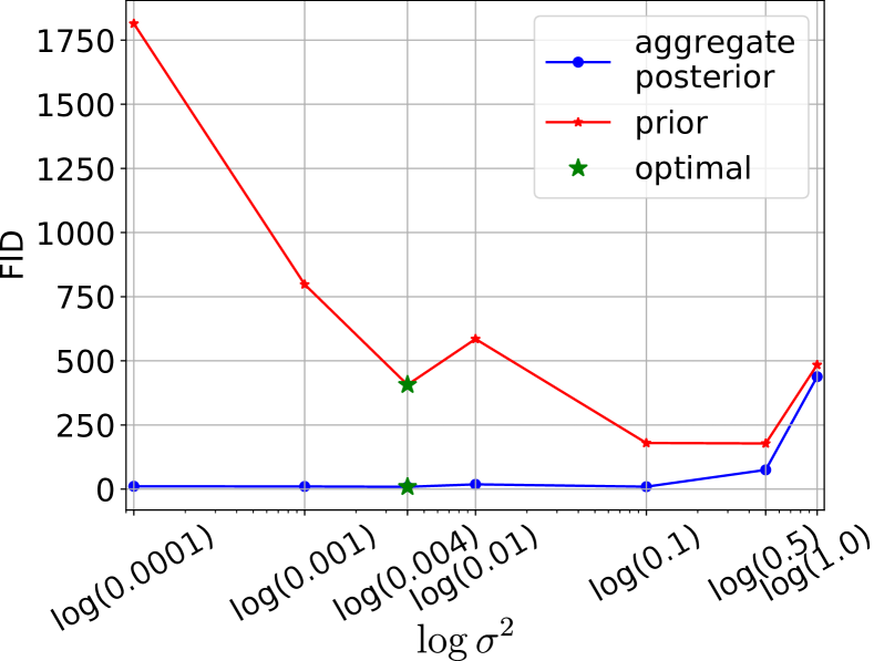
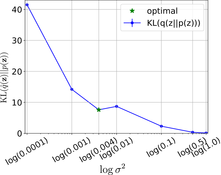
Here we compare the learned VAE models under 3 metrics: 1) the optimised ELBO value (higher indicates a closer bound to the data log likelihood), 2) FID score (lower indicates a better visual quality of the generated samples (?)) and 3) the KL divergence between the approximate aggregate posterior and the prior (smaller often indicates a simpler and smoother marginal latent distribution). In Figure 1, we show these metrics with $\sigma^{2}$ fixed at 6 different values ranging between 0 and 1 and also trained a VAE model with $\sigma^{2}$ learnt under the ELBO in (8) for the MNIST dataset. When $\sigma^{2}$ is optimised (indicated by a green star), the model achieves the highest ELBO, one of the lowest FID scores and still remains reasonably close to the prior distribution. In Figure 1(b), we plot the FID scores evaluated with samples drawn from the approximate posterior (blue) and the prior (red). For all cases the sample quality from aggregate posterior is better than that from the prior distribution and the gap grows exponentially as $\sigma^{2}$ gets smaller.

We also compared the model performance under our proposal (learning $\sigma^{2}$) with four other learning methods, including the original VAE ($\sigma^{2}$=0.5), $\beta$-VAE (($\sigma^{2}$=1), DIP-VAE ((?)) and WAE (?) in terms of the generated sample quality measured by FID scores for all three datasets. All methods adopt the same model architecture. The result is given in Table 2. For all datasets, optimising $\sigma^{2}$ achieves the best FID score. Examples of generated samples are given in Supplemental Materials.

(a) A significant gap between the aggregate posterior (blue) and prior (orange) distributions consistently exists across all methods.

(b) Samples generated from approximate aggregate posterior (top) or prior distribution (bottom) for CelebA dataset.

Figure 2: Gap between aggregate posterior and prior distributions causes bad quality samples to be generated from the prior.

Finally, for VAE models with relatively low latent dimensions, we are able to evaluate the IWAE test log likelihood (LL) (?), which is proposed as a tighter lower bound to the log likelihood $\log p({\mathbf{x}})$ than ELBO and hence will give a better evaluation on how well the model is optimised in terms of approaching the data log likelihood objective. In Table 3, we list the IWAE test LL evaluated over 500 test data samples with 20 importance points per sample for the MNIST and fashion MNIST datasets where a VAE model of 16-dimensional latent space is learnt. Optimising $\sigma^{2}$ significantly improves the test LL in comparison to other learning methods. More interestingly, there is a huge performance boost when $\sigma^{2}$ is estimated across data dimensions and by conditioning on the input data compared to optimising a single-valued $\sigma^{2}$. Therefore, we conclude that using the full learning procedure to predict a more flexible $\sigma^{2}$ estimator gives better results.

5.3 Aggregate Posterior vs Prior

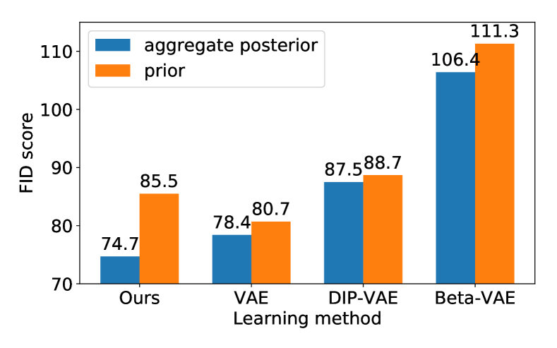
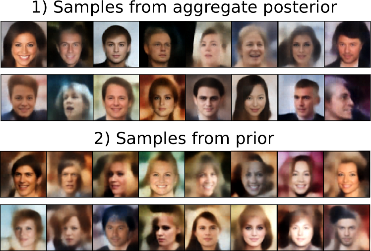
In Figure 2(a), we compared FID scores of generated samples from both approximate aggregate posterior and prior distributions across 4 different methods and it indicates the sample quality is always better if the samples are drawn from the approximate aggregate posterior. In Figure 2(b), samples from both distributions are generated under our proposal for the CelebA dataset. The samples from the aggregate posterior are consistently more realistic, whereas the samples from the prior distribution are either with essential facial feature missing or damaged.

5.4 Uncertainty Estimation

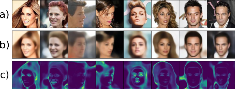
A very powerful application of optimising the $\sigma^{2}$ parameter, especially with the more flexible $\sigma^{2}$ setting where the $\sigma^{2}$ is conditioned on a latent encoding and allowed to be variable across data dimensions, is to estimate uncertainty in the generated samples. Figure 3 illustrates the estimated uncertainty in the reconstructed samples for MNIST and CelebA datasets. Note the predicted $\sigma^{2}$ highlights the region where the reconstruction is different from the original data samples. During training, $\sigma^{2}$ is learnt to suppress the difference between the reconstructed and the original data samples and such difference is highly correlated with the statistical irregularity in the dataset. For example, the major difference between the reconstructed digit zero and its corresponding data sample is at the top where the stroke starts and ends. It is the most unpredictable part of writing a zero and that’s why the model fails to reconstruct this part accurately. Figure 4 illustrates uncertainty estimation in generated samples for both MNIST and CelebA datasets. Notice in Figure 4(b), the high uncertainty regions correspond to eyes, mouths, edges of hair and backgrounds, which are highly variable across the dataset. Such uncertainty estimation indicates that the model is aware that there are many other possibilities to generate these regions and it only renders one of them.

(a) MNIST.

(b) CelebA.

Figure 3: Uncertainty estimation for reconstructed data. a) ground truth images, b) reconstructed images and c) estimated $\sigma^{2}$ indicating uncertainty.

(a) MNIST.

(b) CelebA.

Figure 4: Uncertainty estimation for generated data. a) generated samples and b) estimated uncertainty.

5.5 Ablation Study

A very important hyperparameter in our learning procedure is the number of components in the Gaussian mixture model that we use to estimate the aggregate posterior $q_{\phi}({\mathbf{z}})$. We carried out a study about its impact on the quality of generated samples measured by FID scores for the CelebA dataset and the result is shown in Table 4. Increasing the number of components does not lead to any obvious improvement in the generation quality (FID score is only improves by 1.5 ($<2\%$) when the number of mixtures increases from 500 to 2000). Only when the number of mixture is extremely large, such as 10k, we can see a significant gain, but this is likely to be caused by the approximation becoming overfitted to the 50k samples that we use to fit the mixture model. Therefore, in all of our experiments, we stick with a relatively small number of Gaussian mixtures, specifically 32 for MNIST and fashion MNIST and 500 for CelebA.

Table 4: Study the impact of the number of Gaussian mixtures used in the approximation of the aggregate posterior on the generated sample quality (CelebA dataset).

N mixtures	500	1000	2000	10000
FID	79.9	79.2	78.4	73.1

6 Conclusion

In this paper, we propose a learning algorithm that automatically achieves (for real-valued data) optimal balance between the two competing objectives (reconstruction loss and prior regularisation) for the VAE ELBO loss. A convenient by-product of our learning scheme is an effective uncertainty estimator for the generation or reconstruction prediction, allowing a wider range of potential applications, including safety critical environments. We further study the gap between the aggregate posterior and the prior distribution, which is associated with poor samples being generated, and offer a simple solution to mitigate such problems.

See pages 1-9 of appendix1.pdf See pages 1-6 of appendix2.pdf

References

- Alemi et al. 2017 Alemi, A. A.; Fischer, I.; Dillon, J. V.; and Murphy, K. 2017. Deep variational information bottleneck. In 5th International Conference on Learning Representations, ICLR 2017.
- Alemi et al. 2018 Alemi, A. A.; Poole, B.; Fischer, I.; Dillon, J. V.; Saurous, R. A.; and Murphy, K. 2018. Fixing a broken ELBO. In Proceedings of the 35th International Conference on Machine Learning, ICML 2018, 159–168.
- Bishop 1994 Bishop, C. M. 1994. Mixture density networks.
- Bishop 2006 Bishop, C. M. 2006. Pattern recognition and machine learning. springer.
- Blei, Kucukelbir, and McAuliffe 2016 Blei, D. M.; Kucukelbir, A.; and McAuliffe, J. D. 2016. Variational inference: A review for statisticians. CoRR abs/1601.00670.
- Burda, Grosse, and Salakhutdinov 2015 Burda, Y.; Grosse, R.; and Salakhutdinov, R. 2015. Importance weighted autoencoders.
- Burgess et al. 2018 Burgess, C. P.; Higgins, I.; Pal, A.; Matthey, L.; Watters, N.; Desjardins, G.; and Lerchner, A. 2018. Understanding disentangling in -vae. CoRR abs/1804.03599.
- Cremer, Li, and Duvenaud 2018 Cremer, C.; Li, X.; and Duvenaud, D. 2018. Inference suboptimality in variational autoencoders. CoRR abs/1801.03558.
- Dilokthanakul et al. 2016 Dilokthanakul, N.; Mediano, P. A. M.; Garnelo, M.; Lee, M. C. H.; Salimbeni, H.; Arulkumaran, K.; and Shanahan, M. 2016. Deep unsupervised clustering with gaussian mixture variational autoencoders. CoRR abs/1611.02648.
- Heusel et al. 2017a Heusel, M.; Ramsauer, H.; Unterthiner, T.; Nessler, B.; and Hochreiter, S. 2017a. Gans trained by a two time-scale update rule converge to a local nash equilibrium. In Advances in Neural Information Processing Systems, 6626–6637.
- Heusel et al. 2017b Heusel, M.; Ramsauer, H.; Unterthiner, T.; Nessler, B.; and Hochreiter, S. 2017b. Gans trained by a two time-scale update rule converge to a local nash equilibrium. In Advances in Neural Information Processing Systems, 6626–6637.
- Higgins et al. 2017a Higgins, I.; Matthey, L.; Pal, A.; Burgess, C.; Glorot, X.; Botvinick, M.; Mohamed, S.; and Lerchner, A. 2017a. beta-vae: Learning basic visual concepts with a constrained variational framework. In 5th International Conference on Learning Representations, ICLR 2017.
- Higgins et al. 2017b Higgins, I.; Sonnerat, N.; Matthey, L.; Pal, A.; Burgess, C.; Botvinick, M.; Hassabis, D.; and Lerchner, A. 2017b. SCAN: learning abstract hierarchical compositional visual concepts. CoRR abs/1707.03389.
- Kingma and Welling 2013 Kingma, D. P., and Welling, M. 2013. Auto-encoding variational bayes. CoRR abs/1312.6114.
- Kingma, Salimans, and Welling 2016 Kingma, D. P.; Salimans, T.; and Welling, M. 2016. Improving variational inference with inverse autoregressive flow. CoRR abs/1606.04934.
- Kumar, Sattigeri, and Balakrishnan 2018 Kumar, A.; Sattigeri, P.; and Balakrishnan, A. 2018. Variational inference of disentangled latent concepts from unlabeled observations. In International Conference on Learning Representations.
- LeCun 1998 LeCun, Y. 1998. The mnist database of handwritten digits. http://yann.lecun.com/exdb/mnist/.
- Liu et al. 2015 Liu, Z.; Luo, P.; Wang, X.; and Tang, X. 2015. Deep learning face attributes in the wild. In Proceedings of the 2015 IEEE International Conference on Computer Vision (ICCV), ICCV ’15, 3730–3738. Washington, DC, USA: IEEE Computer Society.
- Mathieu et al. 2019 Mathieu, E.; Rainforth, T.; Siddharth, N.; and Teh, Y. W. 2019. Disentangling disentanglement in variational autoencoders. In Proceedings of the 36th International Conference on Machine Learning, ICML 2019, 4402–4412.
- Ranganath, Tran, and Blei 2016 Ranganath, R.; Tran, D.; and Blei, D. M. 2016. Hierarchical variational models. In Proceedings of the 33nd International Conference on Machine Learning, ICML 2016, 324–333.
- Rasmussen and Williams 2005 Rasmussen, C. E., and Williams, C. K. I. 2005. Gaussian Processes for Machine Learning (Adaptive Computation and Machine Learning). The MIT Press.
- Rezende and Mohamed 2015 Rezende, D. J., and Mohamed, S. 2015. Variational inference with normalizing flows. In Proceedings of the 32nd International Conference on Machine Learning, ICML 2015, 1530–1538.
- Rezende, Mohamed, and Wierstra 2014 Rezende, D. J.; Mohamed, S.; and Wierstra, D. 2014. Stochastic backpropagation and approximate inference in deep generative models. In Proceedings of the 31th International Conference on Machine Learning, ICML 2014, 1278–1286.
- Salimans et al. 2016 Salimans, T.; Goodfellow, I.; Zaremba, W.; Cheung, V.; Radford, A.; and Chen, X. 2016. Improved techniques for training gans. In Advances in neural information processing systems, 2234–2242.
- Suzuki, Nakayama, and Matsuo 2017 Suzuki, M.; Nakayama, K.; and Matsuo, Y. 2017. Joint multimodal learning with deep generative models. In 5th International Conference on Learning Representations, ICLR 2017.
- Tolstikhin et al. 2017 Tolstikhin, I. O.; Bousquet, O.; Gelly, S.; and Schölkopf, B. 2017. Wasserstein auto-encoders. CoRR abs/1711.01558.
- Tomczak and Welling 2016 Tomczak, J. M., and Welling, M. 2016. Improving variational auto-encoders using householder flow. CoRR abs/1611.09630.
- Tomczak and Welling 2018 Tomczak, J. M., and Welling, M. 2018. VAE with a vampprior. In International Conference on Artificial Intelligence and Statistics, AISTATS 2018, 1214–1223.
- Vedantam et al. 2018 Vedantam, R.; Fischer, I.; Huang, J.; and Murphy, K. 2018. Generative models of visually grounded imagination. In 6th International Conference on Learning Representations, ICLR 2018.
- Williams 1992 Williams, R. J. 1992. Simple statistical gradient-following algorithms for connectionist reinforcement learning. Machine Learning 8:229–256.
- Xiao, Rasul, and Vollgraf 2017 Xiao, H.; Rasul, K.; and Vollgraf, R. 2017. Fashion-mnist: a novel image dataset for benchmarking machine learning algorithms. arXiv preprint arXiv:1708.07747.