Boosting Item-based Collaborative Filtering via Nearly Uncoupled Random Walks

Abstract.

Item-based models are among the most popular collaborative filtering approaches for building recommender systems. Random walks can provide a powerful tool for harvesting the rich network of interactions captured within these models. They can exploit indirect relations between the items, mitigate the effects of sparsity, ensure wider itemspace coverage, as well as increase the diversity of recommendation lists. Their potential however, can be hindered by the tendency of the walks to rapidly concentrate towards the central nodes of the graph, thereby significantly restricting the range of $K$-step distributions that can be exploited for personalized recommendations. In this work we introduce RecWalk; a novel random walk-based method that leverages the spectral properties of nearly uncoupled Markov chains to provably lift this limitation and prolong the influence of users’ past preferences on the successive steps of the walk—thereby allowing the walker to explore the underlying network more fruitfully. A comprehensive set of experiments on real-world datasets verify the theoretically predicted properties of the proposed approach and indicate that they are directly linked to significant improvements in top-$n$ recommendation accuracy. They also highlight RecWalk’s potential in providing a framework for boosting the performance of item-based models. RecWalk achieves state-of-the-art top-$n$ recommendation quality outperforming several competing approaches, including recently proposed methods that rely on deep neural networks.

1. Introduction

Recommender Systems are information filtering tools that aim to help users navigate through an ocean of available options and support their decision making process regarding what items to buy, what movies to watch, what articles to read etc. Over the past decade they have become an indispensable component of most e-commerce applications as well as content delivery platforms. Top-$n$ recommendation algorithms are a crucial component of most recommender systems. They provide ranked lists of items tailored to the particular tastes of the users, as depicted by their past interactions within the system.

Item-based methods are among the most popular approaches for top-$n$ recommendation (Sarwar et al., 2001; Ning and Karypis, 2011; Ning et al., 2015). Such methods work by building a model that captures the relations between the items, which is then used to recommend new items that are “close” to the ones each user has consumed in the past. Item-based models have been shown to achieve high top-$n$ recommendation accuracy (Sarwar et al., 2001; Ning and Karypis, 2011) while being scalable and easy to interpret (Ning et al., 2015). The fact, however, that they typically consider only direct inter-to-item relations can impose fundamental limitations to their quality and make them brittle to the presence of sparsity—leading to poor itemspace coverage and significant decay in performance (Adomavicius and Tuzhilin, 2005). Random-walk-based methods are particularly well-suited for alleviating such problems. Having the innate ability to relate items that are not directly connected by propagating information along the edges of the underlying item-to-item graph, random walk methods are more robust to the effects of sparsity and they can afford better coverage of the itemspace. However, their effectiveness in terms of top-$n$ recommendation can be limited by the tendency of the walks to concentrate probability mass towards the central nodes of the graph—thus disproportionately boosting the recommendation scores of popular items in the system. This means that in order to produce high quality recommendations, traditional random-walk-based techniques are restricted to exploit just the first few steps of the walk that are still influenced by the personalized starting distribution. This is in accordance to the mathematical properties of random walks and it has also been empirically verified that when applied to real-world networks, short-length random walks typically work best (Cooper et al., 2014; Christoffel et al., 2015; Eksombatchai et al., 2018).

In this work we introduce RecWalk; a novel framework for top-$n$ recommendations that aims to combine the potential of item-based models to discern meaningful relations between the items, with the inherent ability of random walks to diffuse these relations across the itemspace and exploit the rich network of interactions they shape. RecWalk produces recommendations based on a random walk with node-dependent restarts designed to prolong the influence of the personalized initialization on the successive $K$-step landing probabilities of the walk—thereby eliminating the need of ending the walks early. Intuitively, this gives the walker “more time” to harvest the information captured within the item model before succumbing to the “pull” of central nodes. The proposed random walk construction leverages the spectral properties of nearly uncoupled Markov chains (Courtois, 1977) in order to enforce a time-scale dissociation of the stochastic dynamics of the walk towards equilibrium—thus increasing the number of successive landing probabilities that carry personalized information useful for top-$n$ recommendation. The properties of our model are backed by rigorous theoretical analysis of the mixing characteristics of the walk which we empirically verify that are indeed intertwined with top-$n$ recommendation accuracy. A comprehensive set of experiments on real-world datasets showcase the potential of the proposed methodology in providing a framework for boosting the performance of item models. RecWalk achieves high recommendation quality outperforming state-of-the-art competing approaches, including recently proposed methods relying on deep neural networks.

Open source implementation of the method is available at:

https://github.com/nikolakopoulos/RecWalk

2. Notation and Definitions

2.1. Notation

Vectors are denoted by bold lower-case letters and they are assumed to be column vectors (e.g., $\mathbf{v}$). Matrices are represented by bold upper-case letters (e.g., $\mathbf{Q}$). The $j$-th column and the $i$-th row of matrix $\mathbf{Q}$ are denoted $\mathbf{q}_{j}$ and $\mathbf{q}^{\mathsf{T}}_{i}$, respectively. The $ij$-th element of matrix $\mathbf{Q}$ is denoted as $Q_{ij}$ or $[\mathbf{Q}]_{ij}$ when such choice leads to clearer presentation. We use $\operatorname{diag}(\mathbf{Q})$ to refer to the matrix that has the same diagonal with matrix $\mathbf{Q}$ and zeros elsewhere, and $\operatorname{Diag}(\mathbf{v})$ to denote the matrix having vector $\mathbf{v}$ on its diagonal, and zeros elsewhere. We use a boldface $\bm{\mathrm{1}}$ to denote a vector all the elements of which are equal to 1 (when we need to specify the dimension of such vector, we do so with a subscript, e.g., $\bm{\mathrm{1}}_{n}$). Furthermore, we use $\lVert\cdot\rVert$ to denote a norm that—unless stated otherwise—is assumed to be the Euclidean. Sets are denoted with calligraphic upper-case letters (e.g., $\mathcal{U,V}$). Finally, symbol $\triangleq$ is used in definition statements.

2.2. Definitions

Let $\mathcal{U}=\{1,\dots,U\}$ be a set of users and $\mathcal{I}=\{1,\dots,I\}$ a set of items. Let $\mathbf{R}\in\mathfrak{R}^{U\times I}$ be the user-item interaction matrix; i.e., the matrix whose $ui$-th element is 1 if user $u$ has interacted with item $i$, and 0 otherwise. Each user $u\in\mathcal{U}$ is modeled by a vector $\bm{\mathrm{r}}_{u}^{\mathsf{T}}\in\mathfrak{R}^{I}$ which coincides with the corresponding row of the user-item interaction matrix $\mathbf{R}$; similarly, each item $i\in\mathcal{I}$ will be modeled by a vector $\bm{\mathrm{r}}_{i}\in\mathfrak{R}^{U}$ which coincides with the corresponding column of matrix $\mathbf{R}$. The rows and columns of $\mathbf{R}$ are assumed to be non-zero; i.e., every user has interacted with at least one item, and for every item there exists at least one user who has interacted with it. Finally, we use the term item model to refer to a matrix $\mathbf{W}\in\mathfrak{R}^{I\times I}$ the $ij$-th element of which gives a measure of proximity or similarity between items $i$ and $j$.

3. Random Walks and Item Models

The fundamental premise of the present work is that combining random walks and item models allows for more effective utilization of the information captured in the item model; considering direct as well as transitive relations between the items, and also alleviating sparsity related problems. However, directly applying random walks on item models can lead to a number of problems that arise from their inherent mathematical properties and the way these properties relate to the underlying top-$n$ recommendation task.

Imagine of a random walker jumping from node to node on an item-to-item graph with transition probabilities proportional to the inter-item proximity scores depicted by an item model. If the starting distribution of this walker reflects the items consumed by a particular user $u$ in the past, the probability the walker lands on different nodes after $K$ steps provide an intuitive measure of proximity that can be used to rank the nodes and recommend items to user $u$ accordingly.

Specifically, if $\mathbf{W}$  denotes the item model and

(1) $$\mathbf{S}\triangleq\operatorname{Diag}(\mathbf{W}\bm{\mathrm{1}})^{-1}\mathbf{W}$$

the transition probability matrix of the walk, personalized recommendations for each user $u$ can be produced e.g., by utilizing the $K$-step landing probability distributions of a walk rooted on the items consumed by $u$:

(2) $$\bm{\pi}_{u}^{\mathsf{T}}\triangleq\bm{\phi}_{u}^{\mathsf{T}}\mathbf{S}^{K},\qquad\bm{\phi}_{u}^{\mathsf{T}}\triangleq\tfrac{\bm{\mathrm{r}}_{u}^{\mathsf{T}}}{\lVert\bm{\mathrm{r}}_{u}^{\mathsf{T}}\rVert_{1}}$$

or by computing the stationary distribution of a random walk with restarts on $\mathbf{S}$, using $\bm{\phi}_{u}^{\mathsf{T}}$ as the restarting distribution. The latter approach is the well-known personalized PageRank model (Page et al., 1999) with teleportation vector $\bm{\phi}_{u}^{\mathsf{T}}$ and damping factor $p$, and its stationary distribution can be expressed (Langville and Meyer, 2011) as

(3) $$\bm{\pi}_{u}^{\mathsf{T}}\triangleq\bm{\phi}_{u}^{\mathsf{T}}\sum_{k=0}^{\infty}(1-p)p^{k}\mathbf{S}^{k}.$$

Clearly, both schemes harvest the information captured in the $K$-step landing probabilities

$$\{\bm{\phi}_{u}^{\mathsf{T}}\mathbf{S}^{k}\}_{k=0,1,\dots}.$$

In the former case, the recommendations are produced by using a fixed $K$; in the latter case they are computed as a weighted sum of all landing probabilities, with the $k$-step’s contribution weighted by $(1-p)p^{k}$. But, how do these landing probabilities change as the number of steps $K$ increases? For how long will they still be significantly influenced by user’s prior history as depicted in $\bm{\phi}_{u}^{\mathsf{T}}$?

When $\mathbf{S}$ is irreducible and aperiodic—which is typically the case in practice—the landing probabilities will converge to a unique limiting distribution irrespectively of the initialization of the walk (Grimmett and Stirzaker, 2001). This means that for large enough $K$, the $K$-step landing probabilities will no longer be “personalized” in the sense that they will become independent of the user-specific starting vector $\bm{\phi}_{u}^{\mathsf{T}}$. Furthermore, long before reaching equilibrium, the usefulness of these vectors in terms of recommendation will start to decay as more and more probability mass gets concentrated to the central nodes of the graph—thereby restricting the number of landing probability distributions that are helpful for personalized recommendation. This imposes a fundamental limitation to the ability of the walk to properly exploit the information encoded in the item model.

Motivated by this, here we propose RecWalk; a novel random-walk model designed to give control over the stochastic dynamics of the walk towards equilibrium; provably, and irrespectively of the dataset or the specific item model onto which it is applied. In RecWalk  the item model is incorporated as a direct item-to-item transition component of a walk on the user-item bipartite network. This component is followed by the random walker with a fixed probability determined by a model parameter that controls the spectral characteristics of the underlying walk. This allows for effective exploration of the item model while the influence of the personalized initialization on the successive landing probability distributions remains strong. Incorporating the item model in a walk on the user-item graph (instead of the item graph alone) is crucial in providing control over the mixing properties; and as we will see in the experimental section of this work such mixing properties are intimately linked to improved top-$n$ recommendation accuracy.

4. Proposed Method

4.1. The RecWalk Stochastic Process

We define $\mathcal{G}\triangleq(\{\mathcal{U},\mathcal{I}\},\mathcal{E})$ to be the user-item bipartite network; i.e., the network with adjacency matrix $\mathbf{A}_{\mathcal{G}}\in\mathfrak{R}^{(U+I)\times(U+I)}$ given by

(4) $$\mathbf{A}_{\mathcal{G}}\triangleq\begin{bmatrix}\mathbf{0}&\mathbf{R}\\ \mathbf{R}^{\mathsf{T}}&\mathbf{0}\end{bmatrix}.$$

Consider a random walker jumping from node to node on $\mathcal{G}$. Suppose the walker currently occupies a node $c\in\mathcal{U}\cup\mathcal{I}$. In order to determine the next step transition the walker tosses a biased coin that yields heads with probability $\alpha$ and tails with probability $(1-\alpha)$:

1. If the coin-toss yields heads, then:

   1. if $c\in\mathcal{U}$, the walker jumps to one of the items rated by the user corresponding to node $c$ uniformly at random;

   2. if $c\in\mathcal{I}$, the walker jumps to one of the users that have rated the current item uniformly at random;

2. If the coin-toss yields tails, then:

   1. if $c\in\mathcal{U}$, the walker stays put;

   2. if $c\in\mathcal{I}$, the walker jumps to a related item abiding by an item-to-item transition probability matrix (to be explicitly defined in the following section).

The stochastic process that describes this random walk is defined to be a homogeneous discrete time Markov chain with state space $\mathcal{U}\cup\mathcal{I}$; i.e., the transition probabilities from any given node $c$ to the other nodes, are fixed and independent of the nodes visited by the random walker before reaching $c$.

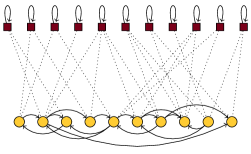
Figure 1. Illustration of the RecWalk  Model. Maroon nodes correspond to users; Gold nodes correspond to items. The dashed lines depict transitions between users and items, captured by matrix $\mathbf{H}$. The solid lines correspond to node-to-node transitions captured by matrix $\mathbf{M}$.

4.2. The Transition Probability Matrix

The transition probability matrix $\mathbf{P}$ that governs the behavior of our random walker can be usefully expressed as a weighted sum of two stochastic matrices $\mathbf{H}$ and $\mathbf{M}$ as

(5) $$\mathbf{P}\triangleq\alpha\mathbf{H}+(1-\alpha)\mathbf{M}$$

where $0<\alpha<1$, is a parameter that controls the involvement of these two components in the final model. Matrix $\mathbf{H}$ can be thought of as the transition probability matrix of a simple random walk on the user-item bipartite network. Since every row and column of matrix $\mathbf{R}$ are non zero, matrix $\mathbf{H}$ is well-defined and it can be expressed as

(6) $$\mathbf{H}\triangleq\operatorname{Diag}(\mathbf{A}_{\mathcal{G}}\bm{\mathrm{1}})^{-1}\mathbf{A}_{\mathcal{G}}.$$

Matrix $\mathbf{M}$, is defined as

(7) $$\mathbf{M}\triangleq\begin{bmatrix}\mathbf{I}&\mathbf{0}\\ \mathbf{0}&\mathbf{M}_{\mathcal{I}}\end{bmatrix}$$

where $\mathbf{I}\in\mathfrak{R}^{U\times U}$ the identity matrix and $\mathbf{M}_{\mathcal{I}}\in\mathfrak{R}^{I\times I}$ a transition probability matrix designed to capture relations between the items. In particular, given an item model with non-negative weights $\mathbf{W}$  we define this matrix using the following stochasticity adjustment strategy:

(8) $$\mathbf{M}_{\mathcal{I}}\triangleq\frac{1}{\lVert\mathbf{W}\rVert_{\infty}}\mathbf{W}+\operatorname{Diag}(\bm{\mathrm{1}}-\frac{1}{\lVert\mathbf{W}\rVert_{\infty}}\mathbf{W}\bm{\mathrm{1}}).$$

The first term divides all the elements by the maximum row-sum of $\mathbf{W}$ and the second enforces stochasticity by adding residuals to the diagonal, appropriately. The motivation behind this definition is to retain the information captured by the relative differences of the item-to-item relations in $\mathbf{W}$, ensuring that

$$[\mathbf{W}]_{ij}\geq[\mathbf{W}]_{i^{\prime}j^{\prime}}\Rightarrow[\mathbf{M}_{\mathcal{I}}]_{ij}\geq[\mathbf{M}_{\mathcal{I}}]_{i^{\prime}j^{\prime}},\qquad\text{for all }i\neq j,i^{\prime}\neq j^{\prime}.$$

This prevents items that are loosely related to the rest of the itemspace to disproportionately influence the inter-item transitions and introduce noise to the model.

An illustration of the RecWalk model is given in Fig 1.

4.3. Choice of the core Item-model

The construction of matrix $\mathbf{W}$ itself can be approached in several ways depending on the available information, the characteristics of the underlying recommendation problem, the properties of matrix $\mathbf{R}$, etc. The fact that random walk methods can achieve naturally itemspace coverage allows us to define this component in a way that promotes sparsity in the relations between the items, having also the advantage to be easy to compute.

In particular, we propose the use of a locally restricted variant of the well-known SLIM method (Ning and Karypis, 2011) that is forced to consider only fixed-size neighborhoods when learning relations between the items. Concretely, for any given item $i$ we find the set of its $C$ closest neighbors (in terms of cosine similarity between their vector representations) and we form a matrix $\mathbf{N}_{i}\in\mathfrak{R}^{U\times C}$, by selecting the corresponding columns of the initial matrix $\mathbf{R}$. We then solve for each item the optimization problem

(9) $$\begin{array}[]{ll}{\displaystyle\operatorname*{minimize}_{\bm{\mathrm{x}}\in\mathfrak{R}^{C}}}&\frac{1}{2}\lVert\bm{\mathrm{r}}_{i}-\mathbf{N}_{i}\bm{\mathrm{x}}\rVert^{2}_{2}+\gamma_{1}\lVert\bm{\mathrm{x}}\rVert_{1}+\frac{1}{2}\gamma_{2}\lVert\bm{\mathrm{x}}\rVert^{2}_{2}\\ \text{subject to}&\bm{\mathrm{x}}\geq\mathbf{0}\end{array}$$

and we fill the corresponding elements in the $i$-th column of matrix $\mathbf{W}$.

The estimation of $\mathbf{W}$ can be performed column-wise, in parallel, and it can be implemented efficiently by exploiting the sparsity of $\mathbf{N}_{i}$, e.g., using coordinate descent (Ning et al., 2019). Note that the size of the per-column optimization problems is controlled by the choice of the numbers of neighbors to be considered (i.e.,$C$), thereby, making estimation of $\mathbf{W}$ scalable to larger itemsets.

The complete procedure for building a RecWalk model is given in Algorithm 1.

Algorithm 1 RecWalk Model

Input: Input matrix $\mathbf{R}$,

       parameters: $\alpha$, $\gamma_{1}$, $\gamma_{2}$, $C$.

Output: RecWalk transition probability matrix $\mathbf{P}$.

parfor  $i\in\mathcal{I}$  do

     Find the $C$ nearest neighbors of item $i$ and form $\mathbf{N}_{i}$

$$\qquad\ \ \begin{array}[]{ll}{\displaystyle\operatorname*{minimize}_{\bm{\mathrm{x}}\in\mathfrak{R}^{C}}}&\frac{1}{2}\lVert\bm{\mathrm{r}}_{i}-\mathbf{N}_{i}\bm{\mathrm{x}}\rVert^{2}_{2}+\gamma_{1}\lVert\bm{\mathrm{x}}\rVert_{1}+\frac{1}{2}\gamma_{2}\lVert\bm{\mathrm{x}}\rVert^{2}_{2}\\ \text{subject to}&\bm{\mathrm{x}}\geq\mathbf{0}\end{array}$$

     Fill the corresponding elements in the $i-$th column of $\mathbf{W}$.

end parfor

$\mathbf{M}_{\mathcal{I}}\leftarrow\frac{1}{\lVert\mathbf{W}\rVert_{\infty}}\mathbf{W}+\operatorname{Diag}(\bm{\mathrm{1}}-\frac{1}{\lVert\mathbf{W}\rVert_{\infty}}\mathbf{W}\bm{\mathrm{1}})$

$\mathbf{A}_{\mathcal{G}}\leftarrow\begin{bmatrix}\mathbf{0}&\mathbf{R}\\ \mathbf{R}^{\mathsf{T}}&\mathbf{0}\end{bmatrix}$

$\mathbf{P}\leftarrow\alpha\operatorname{Diag}(\mathbf{A}_{\mathcal{G}}\bm{\mathrm{1}})^{-1}\mathbf{A}_{\mathcal{G}}+(1-\alpha)\begin{bmatrix}\mathbf{I}&\mathbf{0}\\ \mathbf{0}&\mathbf{M}_{\mathcal{I}}\end{bmatrix}$

4.4. Recommendation Strategies

Having defined the RecWalk transition probability matrix we can produce recommendations by exploiting the information captured in the successive landing probability distributions of a walk initialized in a user-specific way. Here, we will consider two recommendation strategies; namely

RecWalk^K-step::

The recommendation score of user $u$ for item $i$ is defined to be the probability the random walker lands on node $i$ after $K$ steps, given that she started on node $u$. Therefore, the recommendation score for item $i$ is given by the corresponding elements of

(10) $$\bm{\pi}_{u}^{\mathsf{T}}\triangleq\bm{\mathrm{e}}_{u}^{\mathsf{T}}\mathbf{P}^{K}$$

where $\bm{\mathrm{e}}_{u}\in\mathfrak{R}^{U+I}$ is a vector that contains the element 1 on the position that corresponds to user $u$ and zeros elsewhere. The computation of the recommendations is presented in Algorithm 2 and it entails

$$\Theta(K\operatorname{nnz}(\mathbf{P}))$$

operations, where $\operatorname{nnz}(\mathbf{P})$ is the number of nonzero elements in $\mathbf{P}$.

RecWalk^PR::

The recommendation score of user $u$ for item $i$ is defined to be the element that corresponds to item $i$ in the limiting distribution of a random walk with restarts on $\mathbf{P}$, with damping factor $\eta$ and teleportation distribution $\bm{\mathrm{e}}_{u}$:

(11) $$\bm{\pi}_{u}^{\mathsf{T}}\triangleq\lim\limits_{K\to\infty}\bm{\mathrm{e}}_{u}^{\mathsf{T}}(\eta\mathbf{P}+(1-\eta)\bm{\mathrm{1}}\bm{\mathrm{e}}_{u}^{\mathsf{T}})^{K}.$$

This can be computed using the power method as in Algorithm 3. Producing recommendations for a user involves

$$\Theta((\log\epsilon/\log\eta)\operatorname{nnz}(\mathbf{P}))$$

floating point operations for convergence up to a tolerance $\epsilon$ (Meyer and Wessell, 2012).

Algorithm 2 RecWalk^K-step

Input: RecWalk model $\mathbf{P}$, user $u\in\mathcal{U}$.

Output: Recommendation vector $\bm{\pi}_{u}$.

$\bm{\pi}_{u}^{\mathsf{T}}\leftarrow\bm{\mathrm{e}}_{u}^{\mathsf{T}}$

for $k\in 1,\dots,K$ do

     $\bm{\pi}_{u}^{\mathsf{T}}\leftarrow\bm{\pi}_{u}^{\mathsf{T}}\mathbf{P}$

end for

Algorithm 3 RecWalk^PR

Input: RecWalk model $\mathbf{P}$, user $u\in\mathcal{U}$, damping factor $\eta$.

Output: Recommendation vector $\bm{\pi}_{u}$.

$\bm{\mathrm{x}}_{(0)}^{\mathsf{T}}\leftarrow\bm{\mathrm{e}}_{u}^{\mathsf{T}}$

$k\leftarrow 0$

repeat

     $k\leftarrow k+1$

     $\bm{\mathrm{x}}_{(k)}^{\mathsf{T}}\leftarrow\eta\bm{\mathrm{x}}_{(k-1)}^{\mathsf{T}}\mathbf{P}+(1-\eta)\bm{\mathrm{e}}_{u}^{\mathsf{T}}$

     Normalize $\bm{\mathrm{x}}_{(k)}^{\mathsf{T}}$

until $\lVert\bm{\mathrm{x}}_{(k)}^{\mathsf{T}}-\bm{\mathrm{x}}_{(k-1)}^{\mathsf{T}}\rVert_{1}<\mathit{tol}$

$\bm{\pi}_{u}\leftarrow\bm{\mathrm{x}}_{(k)}$

5. Theoretical Properties

As we will show in this section, a key property of the RecWalk model is that for small values of parameter $\alpha$ the RecWalk chain is going to be nearly uncoupled into a large number of blocks, thereby allowing the random walk process dynamics towards equilibrium to disentangle into a slow-mixing and a fast-mixing component. This implies personalized landing probabilities even when the number of steps gets large.

5.1. Nearly Uncoupled Markov Chains

A nearly uncoupled Markov chain is a discrete time chain whose transition probability matrix is almost block diagonal (Courtois, 1977; Stewart, 1991). Formally, let $\mathbf{Z}\in\mathfrak{R}^{n\times n}$ be the transition probability matrix of an irreducible and aperiodic Markov chain. Matrix $\mathbf{Z}$ can always be written as

$$\mathbf{Z}=\mathbf{Z}^{\star}+\varepsilon\mathbf{C},$$

where $\mathbf{Z}^{\star}$ is a block-diagonal matrix of order $n$, given by

$$\mathbf{Z}^{\star}\triangleq\begin{pmatrix}\mathbf{Z}^{\star}_{11}&\mathbf{0}&\cdots&\mathbf{0}\\ \mathbf{0}&\mathbf{Z}^{\star}_{22}&\ddots&\vdots\\ \vdots&\ddots&\ddots&\mathbf{0}\\ \mathbf{0}&\cdots&\mathbf{0}&\mathbf{Z}^{\star}_{LL}\end{pmatrix}$$

and matrices $\mathbf{Z}^{\star}_{II}$ are irreducible stochastic matrices of order $n(I)$. Hence,

$$n=\sum_{I=1}^{L}{n(I)}$$

and because both $\mathbf{Z}$ and $\mathbf{Z}^{\star}$ are stochastic, the row-sums of $\mathbf{C}$ are zero.

Matrix $\mathbf{C}$ and the non-negative real number $\varepsilon$ are selected such that for all rows it holds

(12) $$\varepsilon\sum_{J\neq I}\sum_{l=1}^{n(J)}[\mathbf{C}_{IJ}]_{ml} =\sum_{J\neq I}\sum_{l=1}^{n(J)}[\mathbf{Z}_{IJ}]_{ml},$$

(13) $$\varepsilon \triangleq\max_{m_{I}}\sum_{J\neq I}\sum_{l=1}^{n(J)}[\mathbf{Z}_{IJ}]_{ml}$$

where we use $[\mathbf{Z}_{IJ}]_{ml}$ to denote the element at the intersection of the $m$-th row and $l$-th column of the $\mathbf{Z}_{IJ}$ submatrix of $\mathbf{Z}$.

Parameter $\varepsilon$ is referred to as the maximum degree of coupling between the blocks. When $\varepsilon$ is sufficiently small, the Markov chain with transition probability matrix $\mathbf{Z}$ is called nearly uncoupled into $L$ blocks (Courtois, 1977).

5.2. Mixing properties of RecWalk

When graph $\mathcal{G}$ is connected the discrete time Markov chain defined by $\mathbf{P}$ is ergodic (see Appendix A for a proof). Thus, as the number of steps $K$ increases the landing probabilities of RecWalk will converge to a limiting distribution. It is well known (see e.g.,(Stewart, 1994)) that the rate of convergence to this distribution depends on the modulus of the subdominant eigenvalue of the transition probability matrix of the walk, which we denote $\lvert\lambda_{2}(\mathbf{P})\rvert$. In particular, the asymptotic rate of convergence to the limiting distribution is the rate at which

$$\lvert\lambda_{2}(\mathbf{P})\rvert^{k}\to 0.$$

Intuitively, the smaller $|\lambda_{2}(\mathbf{P})|$ is, the sooner the landing probability distributions will start yielding recommendation vectors that are “non-personalized,” in the sense that they are similar for all users irrespectively of the items with which they have interacted.

The following theorem sheds more light to the spectral properties of matrix $\mathbf{P}$.

Theorem 5.1.

Let $\mathbf{P}$ be the RecWalk transition probability matrix with $\alpha\in(0,1)$ defined over a connected user-item network $\mathcal{G}$, and also let $\lambda(\mathbf{P})$ be the set of the eigenvalues of $\mathbf{P}$. Irrespectively of the item model used to define matrix $\mathbf{M}_{\mathcal{I}}$ it holds

1. $1-2\alpha\in\lambda(\mathbf{P})$

2. when $\alpha$ is small enough the Markov chain with transition probability matrix $\mathbf{P}$ will be nearly uncoupled into at least $U+1$ blocks.

Proof.

When $\mathcal{G}$ is connected, the stochastic matrix $\mathbf{H}$ is irreducible (Langville and Meyer, 2011). Moreover, since the graph is bipartite a simple random walk on $\mathcal{G}$ results in a periodic Markov chain with period $d=2$. Therefore, from the Perron-Frobenius theorem (Grimmett and Stirzaker, 2001) we get that

$$\lambda_{1}(\mathbf{H}) =1,$$

$$\lambda_{2}(\mathbf{H}) =e^{2i\pi/d}=e^{i\pi}=-1.$$

The so-called Perron eigenvalue $\lambda_{1}(\mathbf{H})$ is associated with the right eigenvector $\bm{1}$; whereas eigenvalue $\lambda_{2}(\mathbf{H})$ with a right eigenvector which we denote $\mathbf{v}$.

The special structure of $\mathbf{H}$ makes it easy to guess the form of the eigenvector $\mathbf{v}$ as well as to verify that it actually denotes an eigenvector of matrix $\mathbf{M}$ too. In particular, we have

$$\mathbf{v}\triangleq[\overbrace{1\quad 1\quad 1\quad\cdots\quad 1}^{\textrm{$|\mathcal{U}|$ user nodes}}\quad\overbrace{-1\quad-1\quad\cdots\quad-1}^{\textrm{$|\mathcal{I}|$ item nodes}}].$$

It is easy to see that $\mathbf{v}$ is indeed an eigenvector of both matrices $\mathbf{H}$ and $\mathbf{M}$. Specifically, we have

(14) $$\mathbf{H}\mathbf{v}=\begin{bmatrix}\mathbf{0}&\mathbf{H}_{12}\\ \mathbf{H}_{21}&\mathbf{0}\end{bmatrix}\begin{bmatrix}\mathbf{1}_{U}\\ -\mathbf{1}_{I}\end{bmatrix}=\begin{bmatrix}-\mathbf{1}_{U}\\ \mathbf{1}_{I}\end{bmatrix}=-\mathbf{v}$$

from which we get that $(-1,\mathbf{v})$ is an eigenpair of matrix $\mathbf{H}$; and

(15) $$\mathbf{M}\mathbf{v}=\begin{bmatrix}\mathbf{I}&\mathbf{0}\\ \mathbf{0}&\mathbf{M}_{\mathcal{I}}\end{bmatrix}\begin{bmatrix}\mathbf{1}_{U}\\ -\mathbf{1}_{I}\end{bmatrix}=\begin{bmatrix}\mathbf{1}_{U}\\ -\mathbf{1}_{I}\end{bmatrix}=\mathbf{v}$$

which implies that $(1,\mathbf{v})$ is an eigenpair of matrix $\mathbf{M}$.

Now consider a non-singular matrix,

(16) $$\mathbf{Q}\triangleq\begin{bmatrix}\mathbf{1}&\mathbf{v}&\mathbf{X}\end{bmatrix},$$

which contains in its first two columns the eigenvectors 1 and $\mathbf{v}$. Also let

(17) $$\mathbf{Q}^{-1}\triangleq\begin{bmatrix}\bm{\mathrm{y}}^{\mathsf{T}}_{1}\\[1.9919pt] \bm{\mathrm{y}}^{\mathsf{T}}_{2}\\[1.9919pt] \mathbf{Y}^{\mathsf{T}}\end{bmatrix}.$$

By definition it holds $\mathbf{Q}^{-1}\mathbf{Q}=\mathbf{I}$, which can be usefully written as

(18) $$\begin{bmatrix}\bm{\mathrm{y}}^{\mathsf{T}}_{1}\mathbf{1}&\bm{\mathrm{y}}^{\mathsf{T}}_{1}\mathbf{v}&\bm{\mathrm{y}}^{\mathsf{T}}_{1}\mathbf{X}\\[1.9919pt] \bm{\mathrm{y}}^{\mathsf{T}}_{2}\mathbf{1}&\bm{\mathrm{y}}^{\mathsf{T}}_{2}\mathbf{v}&\bm{\mathrm{y}}^{\mathsf{T}}_{2}\mathbf{X}\\[1.9919pt] \mathbf{Y}^{\mathsf{T}}\mathbf{1}&\mathbf{Y}^{\mathsf{T}}\mathbf{v}&\mathbf{Y}^{\mathsf{T}}\mathbf{X}\\ \end{bmatrix} = \begin{bmatrix}1&0&\mathbf{0}\\[1.9919pt] 0&1&\mathbf{0}\\[1.9919pt] \mathbf{0}&\mathbf{0}&\mathbf{I}\\ \end{bmatrix}.$$

Now, if we consider the similarity transformation of the RecWalk transition probability matrix, $\mathbf{Q}^{-1}\mathbf{P}\mathbf{Q}$, also taking into consideration the relations (14), (15) and the identities (18), we have

(19) $$\footnotesize\mathbf{Q}^{-1}\mathbf{P}\mathbf{Q} = \alpha\mathbf{Q}^{-1}\mathbf{H}\mathbf{Q}+(1-\alpha)\mathbf{Q}^{-1}\mathbf{M}\mathbf{Q}$$

$$= \alpha\begin{bmatrix}\mathbf{Y}^{\mathsf{T}}_{1}\mathbf{1}&(-1)\mathbf{Y}^{\mathsf{T}}_{1}\mathbf{v}&\mathbf{Y}^{\mathsf{T}}_{1}\mathbf{H}\mathbf{X}\\[1.9919pt] \mathbf{Y}^{\mathsf{T}}_{2}\mathbf{1}&(-1)\mathbf{Y}^{\mathsf{T}}_{2}\mathbf{v}&\mathbf{Y}^{\mathsf{T}}_{2}\mathbf{H}\mathbf{X}\\[1.9919pt] \mathbf{Y}^{\mathsf{T}}\mathbf{1}&(-1)\mathbf{Y}^{\mathsf{T}}\mathbf{v}&\mathbf{Y}^{\mathsf{T}}\mathbf{H}\mathbf{X}\\ \end{bmatrix}+(1-\alpha)\begin{bmatrix}\mathbf{Y}^{\mathsf{T}}_{1}\mathbf{1}&\mathbf{Y}^{\mathsf{T}}_{1}\mathbf{v}&\mathbf{Y}^{\mathsf{T}}_{1}\mathbf{M}\mathbf{X}\\[1.9919pt] \mathbf{Y}^{\mathsf{T}}_{2}\mathbf{1}&\mathbf{Y}^{\mathsf{T}}_{2}\mathbf{v}&\mathbf{Y}^{\mathsf{T}}_{2}\mathbf{M}\mathbf{X}\\[1.9919pt] \mathbf{Y}^{\mathsf{T}}\mathbf{1}&\mathbf{Y}^{\mathsf{T}}\mathbf{v}&\mathbf{Y}^{\mathsf{T}}\mathbf{M}\mathbf{X}\\ \end{bmatrix}$$

$$= \begin{bmatrix}\alpha&0&\alpha\mathbf{Y}^{\mathsf{T}}_{1}\mathbf{H}\mathbf{X}\\[1.9919pt] 0&-\alpha&\alpha\mathbf{Y}^{\mathsf{T}}_{2}\mathbf{H}\mathbf{X}\\[1.9919pt] \mathbf{0}&\mathbf{0}&\alpha\mathbf{Y}^{\mathsf{T}}\mathbf{H}\mathbf{X}\\ \end{bmatrix}+\begin{bmatrix}1-\alpha&0&(1-\alpha)\mathbf{Y}^{\mathsf{T}}_{1}\mathbf{M}\mathbf{X}\\[1.9919pt] 0&1-\alpha&(1-\alpha)\mathbf{Y}^{\mathsf{T}}_{2}\mathbf{M}\mathbf{X}\\[1.9919pt] \mathbf{0}&\mathbf{0}&(1-\alpha)\mathbf{Y}^{\mathsf{T}}\mathbf{M}\mathbf{X}\end{bmatrix}$$

$$= \begin{bmatrix}1&0&\alpha\bm{\mathrm{y}}^{\mathsf{T}}_{1}\mathbf{H}\mathbf{X}+(1-\alpha)\bm{\mathrm{y}}^{\mathsf{T}}_{1}\mathbf{M}\mathbf{X}\\[1.9919pt] 0&1-2\alpha&\alpha\bm{\mathrm{y}}^{\mathsf{T}}_{2}\mathbf{H}\mathbf{X}+(1-\alpha)\bm{\mathrm{y}}^{\mathsf{T}}_{2}\mathbf{M}\mathbf{X}\\[1.9919pt] \mathbf{0}&\mathbf{0}&\alpha\mathbf{Y}^{\mathsf{T}}\mathbf{H}\mathbf{X}+(1-\alpha)\mathbf{Y}^{\mathsf{T}}\mathbf{M}\mathbf{X}\end{bmatrix}$$

Thus, matrix $\mathbf{P}$ is similar to a block upper triangular matrix, the eigenvalues of which are the eigenvalues of its diagonal blocks. From that, we directly establish that $1-2\alpha$ is an eigenvalue of the RecWalk transition matrix $\mathbf{P}$, and the first part of the theorem is proved.

To prove the second part it suffices to show that there exists a partition of the state space of the RecWalk chain into blocks, such that the maximum probability of leaving a block upon a single transition is upper-bounded by $\alpha$ (Stewart, 1991). In particular, consider the partition

(20) $$\mathcal{A}\triangleq\{\{u_{1}\},\{u_{2}\},\dots,\{u_{U}\},\mathcal{I}\}.$$

By definition, in the RecWalk model the probability of leaving $u$ is equal to $\alpha$, for all $u\in\mathcal{U}$. Concretely,

(21) $$\Pr\{\text{jump from}\ u\in\mathcal{U}\ \text{to any}\ j\neq u\}=\sum_{j\neq u}P_{uj}=\sum_{j\neq u}\alpha H_{uj}=\alpha.$$

Similarly, the probability of leaving block $\mathcal{I}$ upon a transition is

(22) $$\Pr\{\text{jump from}\ i\in\mathcal{I}\ \text{to any}\ \ell\notin\mathcal{I}\}=\sum_{\ell\notin\mathcal{I}}P_{i\ell}=\sum_{\ell\notin\mathcal{I}}\alpha H_{i\ell}=\alpha.$$

Therefore, the RecWalk chain can always be decomposed according to $\mathcal{A}$ such that the maximum degree of coupling between the involved blocks is exactly equal to $\alpha$. Hence, choosing $\alpha$ to be sufficiently small ensures that the chain will be nearly uncoupled into (at least) $U+1$ blocks. ∎

Theorem 5.1 asserts that the proposed random walk construction ensures the existence of an eigenvalue equal to $1-2\alpha$. This means that the modulus of the eigenvalue that determines the rate of convergence to the limiting distribution will be at least $1-2\alpha$. Hence, choosing $\alpha$ allows us to ensure that the RecWalk process will converge as slow as we need to increase the number of landing probability distributions that can still serve as personalized recommendation vectors in our model—irrespectively of the particular user-item network or the chosen item model upon which it is built.

Moreover note that the spectral fingerprint of nearly uncoupled Markov chains is the existence of a set of subdominant eigenvalues that are relatively close (but not equal) to 1 (Courtois, 1977). In our case, for small values of $\alpha$ these eigenvalues are expected to be clustered close to the value $1-\alpha$ (cf. (19)). The number of these eigenvalues depicts the number of blocks of states into which the chain is nearly uncoupled. Therefore, subject to $\alpha$ being small the RecWalk chain will have at least $U+1$ eigenvalues clustered near the value 1, and it can be shown (see e.g.,(Stewart, 1991)) that matrix $\mathbf{P}$ can be expressed as

(23) $$\mathbf{P}=\bm{\mathrm{1}}\bm{\pi}^{\mathsf{T}}+\mathbf{T}_{\mathrm{slow}}+\mathbf{T}_{\mathrm{fast}}$$

where $\bm{\pi}^{\mathsf{T}}$ is the stationary distribution of the walk, $\mathbf{T}_{\mathrm{slow}}$ is a slow transient component, and $\mathbf{T}_{\mathrm{fast}}$ is a fast transient component. As $K$ gets large the fast transient term will diminish while the elements of the slow transient term will remain large enough to ensure that the recommendation vectors are not completely dominated by $\bm{\mathrm{1}}\bm{\pi}^{\mathsf{T}}$. Of course, as $K$ gets larger and larger the relative influence of the first term will become stronger and stronger, up to the point where each user is assigned the exact same recommendation vector $\bm{\pi}^{\mathsf{T}}$; however, this outcome will be delayed by the existence of the slow transient term $\mathbf{T}_{\mathrm{slow}}$. Note that in a simple random walk on $\mathbf{W}$ such time-scale dissociation of the stochastic dynamics of the walk is typically absent; and certainly it cannot be guaranteed in advance. On the contrary, the proposed random walk construction in RecWalk provides a clear mechanism to ensure such property, and as we will see in the experimental section of this paper this property alone can lead to significant improvements in top-$n$ recommendation quality compared to what one would get by using the item model directly.

5.3. Coverage

It is often useful to be able to ensure that in principle all items can be recommended to the users. However, due to the sparsity of the user-item feedback matrix, such requirement is many times difficult to satisfy or comes at the expense of accuracy. Moreover, the opaque nature of many of the state-of-the-art approaches for top-n recommendation makes it impossible to guarantee such property in advance.

In case of RecWalk^PR this requirement is easily guaranteed. Before we proceed to the proof of this property, we list the following useful Lemma from (Nikolakopoulos and Garofalakis, 2015a).

Lemma 5.2 ((Nikolakopoulos and Garofalakis, 2015a)).

Let $\mathbf{A}$ be a primitive stochastic matrix and $\mathbf{B}_{1},\mathbf{B}_{2},\dots,\mathbf{B}_{n}$ stochastic matrices; then matrix

$$\alpha\mathbf{A}+\beta_{1}\mathbf{B}_{1}+\dots+\beta_{n}\mathbf{B}_{n}$$

where $\alpha>0$ and $\beta_{1},\dots,\beta_{n}\geq 0$ such that

$$\alpha+\beta_{1}+\dots+\beta_{n}=1$$

is a primitive stochastic matrix.

Proposition 5.3 (RecWalk^PR Coverage Conditions).

When $\mathcal{G}$ is connected the personalized recommendation vectors produced by RecWalk^PR with $\alpha,\eta\in(0,1)$ are guaranteed to provide full itemspace coverage for every user in the system, i.e.,

$$[\bm{\pi}_{u}]_{j}>0,\qquad\forall j\in\mathcal{I},\quad\forall u\in\mathcal{U}.$$

Proof.

Notice that $\bm{\pi}_{u}$ in case of RecWalk^PR is defined as the limiting distribution of a Markov chain with transition probability matrix

(24) $$\eta\mathbf{P}+(1-\eta)\bm{\mathrm{1}}\bm{\mathrm{e}}_{u}^{\mathsf{T}}.$$

Under our assumptions, the RecWalk chain is ergodic (see Proposition A.1 in Appendix) and hence, matrix $\mathbf{P}$ is a primitive stochastic matrix (Meyer, 2000). This makes stochastic matrix (24), a linear combination of a primitive matrix, and the rank-one stochastic matrix, $\bm{\mathrm{1}}\bm{\mathrm{e}}_{u}^{\mathsf{T}}$; thus, Lemma 5.2 applies, and we get that (24) is a primitive stochastic matrix as well.

Therefore, the recommendation vector $\bm{\pi}_{u}$ produced by RecWalk^PR will coincide with the unique dominant left eigenvector of the primitive stochastic matrix (24) (up to rescaling of its entries to sum to 1). However, from the Perron Frobenius theorem, we know that every element of the dominant left eigenvector of primitive matrices is necessarily strictly positive (see e.g., (Meyer, 2000)). Thus, when $\mathcal{G}$ is connected and $\alpha,\eta\in(0,1)$, the recommendation vector $\bm{\pi}_{u}$ produced by RecWalk^PR is guaranteed to assign positive scores to every item in the system, i.e,

$$[\bm{\pi}_{u}]_{j}>0,\qquad\forall j\in\mathcal{I},\quad\forall u\in\mathcal{U}.$$

as needed; and the proof is complete. ∎

RecWalk^K-step can guarantee item-space coverage too, provided that $K$ is sufficiently large for the walk to discover the complete set of items. This is a direct consequence of the primitivity of $\mathbf{P}$. Bounding the necessary number of steps $K$ to ensure coverage would require analysis of relevant combinatorial invariants of the particular user-item network and item-model under consideration, and thus, goes beyond the scope of this work. In practice, we find that even modest values of $K$ are enough to ensure such property for every dataset we experimented with. Importantly, we also find that for RecWalk item-space coverage does not come at the expense of accuracy, as it is the case for other item-based recommendation algorithms.

6. Experimental Setting

6.1. Datasets

Our qualitative evaluation is based on six real-world publicly available datasets; namely (i) the movielens dataset which contains the ratings of users for movies and it has been used extensively for the evaluation of top-$n$ recommendation methods; (ii) the yahoo dataset which is a subset of the Yahoo!R2Music dataset (obtained from (Nikolakopoulos et al., 2014)) containing the ratings of users for songs; (iii) the electronics dataset (He and McAuley, 2016) which contains review scores of electronic products in Amazon (we keep users that have rated at least 10 items, and items that have been rated by at least 20 users); (iv) the movies&tv dataset (He and McAuley, 2016) which contains review scores of movies and tv shows in Amazon (we keep users that have scores at least 15 items, and items that have been scored by at least 30 users), (vi) books datasets (He and McAuley, 2016), which contain review scores of books in Amazon (we keep users that have provided review scores for at least 15 books, and books that have been scored by at least 30 users); and (vi) the pinterest dataset (obtained from (He et al., 2017)) which captures the interactions of users regarding images where each interaction denotes whether the user has “pinned” the image to her own board. Basic statistics about the datasets can be found in Table 1.

Table 1. Statistics of datasets used to assess recommendation accuracy.

Name	#users	#items	#interactions		density
electronics	3,769	1,598	66,060		0.0109
movielens	6,040	3,706	1,000,029		0.0447
yahoo	7,307	3,312	404,745		0.0167
movies&tvasdf asdf	10,039	5,400	437,763		0.0081
books	43,550	24,811	1,777,072		0.0016
pinterest	55,187	9,916	1,463,581		0.0027

Furthermore, to assess the scalability of our method we make use of several larger datasets from the collection (He and McAuley, 2016). Their characteristics can be found in Appendix C.

6.2. Evaluation Methodology and Metrics

To evaluate the top-$n$ recommendation performance, we adopted the widely used leave-one-out evaluation protocol (Rendle et al., 2009; Ning and Karypis, 2011; He et al., 2017; Nikolakopoulos et al., 2019; Koren, 2010). In particular, for each user we randomly select one item she liked and we create a test set $\mathcal{T}$. The rest of the dataset is used for training the models. For model selection we repeat the same procedure on the training data and we create a validation set $\mathcal{V}$; and for each method considered we explore the hyperparameter space to find the model that yields the best performance in recommending the items in $\mathcal{V}$, and then we evaluate its out-of-sample performance based on the held-out items in $\mathcal{T}$. For the evaluation we consider for each user her corresponding test item alongside 999 randomly sampled unseen items and we rank the 1000 item lists based on the recommendation scores produced by each method. During training of all competing methods we consider only binary feedback.

The evaluation of the top-$n$ recommendation performance is based on three widely used ranking-based metrics; namely the hit ratio (HR@$n$), the average reciprocal hit rank (ARHR@$n$), and the truncated normalized discounted cumulative gain (NDCG@$n$) over the set of users (for a detailed definition we refer the reader to e.g., (Liang et al., 2018; Nikolakopoulos et al., 2019)). For each user, all metrics compare the predicted rank of the held-out item with the ideal recommendation vector which ranks the held-out item first among the items in each user’s test-set list. For all competing methods we get the predicted rank by sorting the recommendation scores that correspond to the items included in each user’s test-set list. While HR@$n$ gives a perfect score if the held-out item is ranked within the first $n$, ARHR@$n$ and NDCG@$n$ use a monotonically increasing discount to emphasize the importance of the actual position of the held-out item in the top-$n$ recommendation list.

7. Experimental Results

7.1. Effect of Parameter $\alpha$

The theoretical analysis of our method suggests that parameter $\alpha$ controls the convergence properties of the RecWalk process and it can be chosen to enable a time-scale dissociation of the stochastic dynamics towards equilibrium that ensures a larger number of personalized landing distributions. Here we verify experimentally the predicted properties and we evaluate their effect on the recommendation quality of the $K$-step landing probabilities.

We build the item model $\mathbf{W}$ that yields the best performance on the validation set and we use it to create matrix $\mathbf{M}_{\mathcal{I}}$ as in (8). We then build the RecWalk model as in Algorithm 1, we run it for different values of $\alpha$ ranging from 0.005 to 0.5, and we report: (i) the performance in terms of average NDCG$@n$ (for $n=10$) across all users for values of steps $K$ up to 30 (Fig.2-A); (ii) the spectra of the corresponding transition probability matrices $\mathbf{P}$ (Fig.2-B); (iii) the peak performance per parameter $\alpha$ along with the step for which it was achieved (Fig.2-C); and (iv) the performance of RecWalk with respect to using the base model $\mathbf{W}$ directly (Fig.2-D).

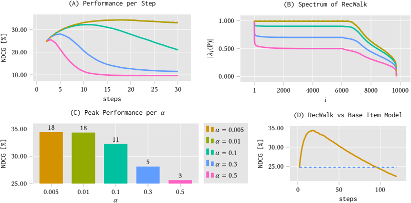
Figure 2. Fig (A) reports the performance of RecWalk in terms of NDCG@10 as a function of the steps for different values of the parameter $\alpha$. Fig (B) plots the spectrum of the RecWalk transition probability matrix for different values of $\alpha$. Fig (C) reports the peak performance for the different values of $\alpha$, as well as the number of steps for which it is achieved (on top of each bar). Fig (D) reports RecWalk performance (with $\alpha$ fixed at 0.005) for different number of steps compared to the performance one would get using the item model directly (blue dashed line).

We find that as the value of $\alpha$ gets smaller the top-$n$ recommendation quality increases and stabilizes for $\alpha<0.01$. Similarly the number of steps that yield the best performance increase (see Fig.2-C). The spectrum of the corresponding transition probability matrices reflects the theoretically predicted properties of the model. Indeed for very small values of $\alpha$ we observe that the subdominant eigenvalues cluster near the value $1$, thus forming the slowly varying component of matrix $\mathbf{P}$, which ensures that the successive landing probabilities of the random walk are influenced by the initial state for longer. Furthermore, we find that the proposed methodology entails a significant increase in performance with respect to what one would get by using the proposed base item-model directly. In particular the recommendation performance of the $K$-step landing probabilities of RecWalk overpasses the performance of the base model (see Fig.2-D) for a wide range of steps up to a maximum increase of 39.09% for $K=18$ steps. Finally, notice that when the number of steps becomes very large the recommendation performance decays, as every $\bm{\pi}_{u}$ starts to converge to the same stationary distribution $\bm{\pi}$. In other words, as $K$ gets larger and larger similar recommendations will be produced for every user in the system. Due to the mixing properties of the RecWalk chain, however, one can ensure that such outcome will not occur for small $K$—thereby allowing RecWalk to effectively explore the underlying network without losing focus of the user-specific initialization.

Our results suggest that the mixing properties of the RecWalk chain are indeed intertwined with the top-$n$ recommendation quality and can lead to a significant boost in performance. This justifies the intuition that motivated the particular design of the walk. For additional experiments regarding the effects of sparsity on the performance of RecWalk see Appendix D.

7.2. RecWalk as a Framework

In the definition of the inter-item transition probability matrix we proposed a particular strategy for constructing matrix $\mathbf{W}$ that was designed to promote locality on the direct item-to-item transitions while being easy to compute. Instead of this particular matrix $\mathbf{W}$ one could use any model that captures inter-item relations. But does our approach offer any benefit with respect to performing simple random walks on the corresponding item-model or to simply using the item model directly?

Here we explore this question by empirically evaluating two commonly used item models. Namely:

1. a cosine similarity model $\mathbf{W}_{\textsc{cos}}$ defined such that its $ij$-th element is given by $\bm{\mathrm{r}}_{i}^{\mathsf{T}}\bm{\mathrm{r}}_{j}/(\lVert\bm{\mathrm{r}}_{i}\rVert\lVert\bm{\mathrm{r}}_{j}\rVert)$;

2. a SLIM model which learns a matrix $\mathbf{W}_{\textsc{slim}}$ by solving an $\ell_{1},\ell_{2}$ regularized optimization problem (see (Ning and Karypis, 2011) for details).

We consider the respective base models alongside six approaches based on random walks; namely

1. SRW, which recommends using the $K$-step distribution of a simple random walk on $\mathbf{W}$ with transition probability matrix $\mathbf{S}$ initialized with $\bm{\phi}_{u}^{\mathsf{T}}$ as in (2);

2. PR, which produces recommendations based on $\mathbf{S}$ as in (3);

3. RecWalk^K-step;

4. RecWalk^PR;

5. RecWalk$[\mathbf{M}_{\mathcal{I}}]$^K-step, which produces recommendations as in (2) but using the RecWalk inter-item transition probability matrix introduced in (8) instead of $\mathbf{S}$;

6. RecWalk$[\mathbf{M}_{\mathcal{I}}]$^PR, which produces recommendations as in (3) using RecWalk’s $\mathbf{M}_{\mathcal{I}}$ instead of $\mathbf{S}$.

Table 2. Top-n Recommendation Quality under Different Random Walk Constructions

Method	COS	SLIM
Base model asdfa asdf asdf adf asdg asdf asdf asdfas dfas	17.61	27.28
SRW	17.82	25.37
PR	18.11	25.37
RecWalkK-step	20.52	31.87
RecWalkPR	20.33	31.80
RecWalk$[\mathbf{M}_{\mathcal{I}}]$K-step	17.85	31.41
RecWalk$[\mathbf{M}_{\mathcal{I}}]$PR	20.27	31.78

• Hyperparameters: SRW: K$\in\{1,\dots,50\}$; PR: $p\in\{0.1,\dots,0.9\}$; SLIM: $\lambda,\beta\in\{0.1,0.5,1,3,5,10,20\}$; RecWalk: $\alpha=0.005$ and $K\in\{1,\dots,30\}$ for RecWalk^K-step  and $\eta\in\{0.1,0.2,\dots,0.9\}$ for RecWalk^PR.

We run all models on the movielens dataset and in Table 2 we report their performance on the NDCG@$n$ metric. We see that RecWalk^K-step  and RecWalk^PR  were able to boost the performance of both item models (up to +16.52% for COS and +16.82% for SLIM) with the performance difference between the two variants being insignificant. Applying simple random walks (SRW) or random walks with restarts (PR) directly to the row-normalized version of the item graph does not perform well (+2.84% in case of COS and -7% in case of SLIM). In particular in the case of SRW we observed a rapid decay in performance (after the first step for SLIM and after the first few steps for COS); similarly in case of PR the best performance was obtained for very small values of $p$—essentially enforcing the $K$-step landing probabilities after the first few steps to contribute negligibly to the production of the recommendation scores (cf. (3)). Using RecWalk’s inter-item transition probability matrix alone, on the other hand, performed very well especially when we use the SLIM model as a base.

To gain more insight into the observed differences in performance of the walks on the item graphs, we also plot the spectra of the transition probability matrices $\mathbf{M}_{\mathcal{I}}$, alongside the spectra of the respective matrices $\mathbf{S}$  (Fig. 3). We see that in case of $\mathbf{S}$ the magnitude of the eigenvalues cause the walks to mix very quickly. In case of matrix $\mathbf{M}_{\mathcal{I}}$ on the other hand, the eigenvalues decay more gracefully and on the SLIM graph in particular, there appears to be a large number of eigenvalues near 1, which delay the convergence of the landing distributions towards equilibrium. This effect is not as pronounced in case of COS which is reflected in the small increase in performance in case of RecWalk$[\mathbf{M}_{\mathcal{I}}]$^K-step.

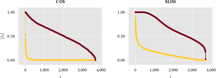
Figure 3. The figure plots the spectra of the transition probability matrices $\mathbf{S}$ (gold line) and $\mathbf{M}_{\mathcal{I}}$ (maroon line) defined using the corresponding item models.

Again our experiments reveal a clear connection between the mixing properties of the walks and their potential in achieving good recommendation quality. Note also that the stochasticity adjustment strategy proposed in (8) seems to promote slow mixing in itself. However, using $\mathbf{M}_{\mathcal{I}}$ alone cannot in general guarantee this property irrespectively of the underlying item model whereas using the complete RecWalk model can give absolute control over convergence (as Theorem 5.1 predicted).

Table 3. Top-$n$ recommendation quality of the competing approaches in terms of HR@10, ARHR@10 and NDCG@10.

		movielens				yahoo
Method		AHR[%]R	ARHR[%]	NDCG[%]		AHR[%]R	ARHR[%]	NDCG[%]
PureSVD		44.14	19.33	25.36		38.68	18.30	22.62
SLIM		46.34	21.39	27.28		52.24	23.21	30.03
EigenRec		45.21	20.44	26.35		48.12	23.30	29.23
Mult-DAE		44.06	18.97	24.83		45.37	21.46	27.07
Mult-VAE		44.35	19.50	25.31		45.09	21.22	26.80
APR		42.45	18.69	24.24		44.75	19.50	25.36
RP3b		34.87	15.02	19.66		41.51	17.82	22.94
NAIS		46.36	20.65	26.68		50.53	23.64	29.91
RecWalkK-step		50.28	27.20	33.13		55.02	28.94	35.10
RecWalkPR		52.52	27.74	33.57		54.78	28.71	34.87

		pinterest				movies&tv
Method		AHR[%]R	ARHR[%]	NDCG[%]		AHR[%]R	ARHR[%]	NDCG[%]
PureSVD		30.97	11.85	16.30		22.58	09.88	12.86
SLIM		34.17	13.63	18.57		27.26	12.95	16.37
EigenRec		33.81	13.51	18.41		25.22	11.44	14.66
Mult-DAE		35.03	13.79	18.77		27.10	11.96	15.50
Mult-VAE		35.13	13.73	18.71		26.72	12.05	15.40
APR		33.93	13.11	17.94		22.99	09.46	12.58
RP3b		27.01	8.07	12.45		26.52	11.79	15.22
NAIS		34.06	12.95	17.82		24.35	10.87	13.99
RecWalkK-step		35.38	14.07	18.95		28.34	12.99	16.51
RecWalkPR		35.29	14.07	19.00		28.15	13.13	16.51

		books				electronics
Method		AHR[%]R	ARHR[%]	NDCG[%]		AHR[%]R	ARHR[%]	NDCG[%]
PureSVD		46.84	25.84	30.81		9.60	3.71	5.07
SLIM		56.72	34.50	39.67		13.64	6.05	7.85
EigenRec		52.89	29.36	34.93		11.83	4.68	6.34
Mult-DAE		54.66	29.75	35.60		13.40	5.10	7.18
Mult-VAE		53.85	29.24	35.08		13.43	5.56	7.32
APR		51.12	24.96	31.10		11.91	4.37	6.11
RP3b		55.60	31.68	37.35		14.49	6.08	8.03
NAIS		51.18	28.36	33.65		12.68	5.17	6.84
RecWalkK-step		57.73	34.71	40.05		14.65	6.25	8.05
RecWalkPR		57.73	34.65	39.94		14.25	6.18	7.96

• Hyperparameters: RecWalk: (fixed) $\alpha=0.005$, $C=\{2.5\%,5\%,7.5\%,10\%,25\%\}\text{ of }|\mathcal{I}|$, $\gamma_{1}\in\{1,3,5,10\},\gamma_{2}\in\{0.1,0.5,1,3,5,7,9,11,15,20\}$ and $K\in\{3,\dots,20\}$; for RecWalk^PR $\eta=\{0.05,\dots,0.95\}$. PureSVD: $f\in\{10,20,\dots,1000\}$. RP3b: $b\in\{0,0.05,\dots,1\}$. SLIM: We used the implementation (Ning et al., 2019), $\lambda,\beta\in\{0.1,0.5,1,3,5,10,20\}$. EigenRec: $f\in\{10,20,\dots,1000\},d\in\{-2,-1.95,\dots,2\}$. Mult-DAE- Mult-VAE: we used the hyperparameter tuning approach provided by the authors in their publicly available implementation; we considered both architectures proposed in (Liang et al., 2018); namely $[I-200-I]$ and $[I-600-200-600-I]$. APR: We used the implementation provided by (He et al., 2018a), considering the hyperparametric setting discussed therein; NAIS: We used the implementation provided by (He et al., 2018b), considering the parametric ranges discussed in the paper, namely $\alpha,k\in\{8,16,32,64\}$, $\beta=0.5$ and regularization parameters $\lambda\in\{10^{-6},\dots,1\}$.

7.3. Performance against Competing Approaches

We evaluate the top-$n$ recommendation accuracy of RecWalk^K-step  and RecWalk^PR  against eight competing approaches; namely

1. the well-known PureSVD  method (Cremonesi et al., 2010), which produces recommendations based on the truncated SVD of $\mathbf{R}$;

2. the well-known item-based method SLIM (Ning and Karypis, 2011) which builds a sparse item model by solving an $\ell_{1},\ell_{2}$-regularized optimization problem;

3. the random-walk approach RP3b (Christoffel et al., 2015), which recommends based on a short-length walk on the user-item graph after rescaling the landing probabilities to compensate for the inherent bias of the walk towards popular items;

4. the EigenRec  method (Nikolakopoulos et al., 2019), which builds a factored item model based on a scaled cosine similarity matrix;

5. Mult-VAE and Mult-DAE  (Liang et al., 2018) which extend variational and denoising autoencoders to collaborative filtering using a multinomial likelihood and were shown to achieve state-of-the-art recommendation quality, outperforming several other deep-network-based approaches;

6. APR  (He et al., 2018a), which extends the popular pairwise ranking method BPR (Rendle et al., 2009) by incorporating adversarial training;

7. NAIS (He et al., 2018b), which generalizes the well-known FISM (Kabbur et al., 2013) recommendation algorithm employing an attention mechanism;

7.3.1. Results

Table 3 reports the top-$n$ recommendation performance of the competing approaches. The performance was measured in terms of HR@$n$, ARHR@$n$ and NDCG@$n$, focusing on the $n=10$. Model selection was performed for each dataset and metric following the procedure detailed in Section 6.2 and considering for each method the hyperparameters reported on Table 3.

From the deep network methods, NAIS, Mult-VAE, Mult-DAE manage to perform very well, with the latter two showing more consistent performance across datasets. At the same time Mult-VAE, Mult-DAE where significantly more efficient to compute than NAIS (50x-200x faster training time per epoch). SLIM, does remarkably well in all cases, managing to reach and surpass the performance of deep nets in most datasets (except Mult-VAE and Mult-DAE in pinterest). From the simple latent factor models EigenRec performed well in several cases, while also being very efficient and scalable. RP3b did remarkably well in movies&tv, books, and especially electronics, where it was found to perform better than every method except RecWalk^K-step; its performance in movielens, yahoo and pinterest, however, was not competitive to the neural nets and EigenRec.

We see that both variants of RecWalk perform very well on every metric and for all datasets. The results indicate the potential of the proposed methodology in achieving high quality top-$n$ recommendations.

Importantly, the best performing RecWalk^K-step models also managed to ensure excellent itemspace coverage. This is in contrast to SLIM, where coverage and accuracy do not necessarily go hand-in-hand (a comparison of the coverage properties of RecWalk^K-step and SLIM can be found in Appendix B).

7.4. Runtimes

Table 4 reports the wall-clock timings for training RecWalk, as well as the rest of the competing methods included in Table 3.

Table 4. Training runtimes of the competing methods on the datasets considered in Table 3.

	movielens	yahoo	pinterest	movies&tv	books	electronics
RP3b	¡1s	¡1s	¡1s	¡1s	¡1s	¡1s
PureSVD	¡1s	¡1s	8.1s	¡1s	1.5m	¡1s
EigenRec	¡1s	¡1s	6.8s	2.1s	1.5m	¡1s
Mult-VAE	7.9m	9.1m	1.7h	14.5m	2.8h	3.9m
Mult-DAE	7.2m	8.3m	1.6h	13.1m	2.7h	3.7m
NAIS	6.3h	2.1h	7.3h	4.3h	21.2h	12.6m
SLIM	20.9s	14.7s	14s	29.4s	2.5m	1.1s
APR	6.9h	4.1h	50h	5h	51.7h	43.3m
RecWalk	2s	1.3s	9s	2.1s	21s	¡1s

• Experiments are ran on a single Intel Xeon Gold 6148 CPU @ 2.40GHz Machine with 20 cores and 64Gb DDR4 RAM.

Notice that RecWalk can be trained significantly faster than the deep-net-based alternatives—attaining runtimes comparable to highly efficient methods like PureSVD and EigenRec. Further training times of RecWalk on datasets with large itemspaces can be found in Appendix C.

8. Related Work

Neighborhood-based methods (Ning et al., 2015) and in particular item-based models (Deshpande and Karypis, 2004; Ning and Karypis, 2011) are among the most popular and effective approaches to tackle the top-$n$ recommendation task. A notable such example is SLIM (Ning and Karypis, 2011) which generalizes the traditional item-based CF approaches (Sarwar et al., 2001) to learn a sparse linear item-to-item model. SLIM has been shown repeatedly to yield state-of-the-art top-$n$ recommendation accuracy, and has inspired the proposal of several new methods in recent years (Zheng et al., 2014; Ning and Karypis, 2012; Steck, 2019). Despite their success, however, item-based models are known to be negatively impacted by sparsity which can lead to decay in recommendation performance and poor itemspace coverage. Latent Space methods (Cremonesi et al., 2010; Nikolakopoulos et al., 2019; Hu et al., 2008; Koren, 2010; Weston et al., 2013) are particularly well-suited to alleviate such problems. Generally speaking, the methods of this family work by projecting the elements of the recommender database into a denser subspace that captures their most salient features, giving them the ability to relate previously unrelated elements, and thus making them less vulnerable to sparsity (Nikolakopoulos et al., 2019). Another family of approaches that are able to address issues related to sparsity and poor itemspace coverage are Graph-Based methods (Fouss et al., 2012; Kang et al., 2016; Christoffel et al., 2015; Cooper et al., 2014). The innate characteristic that makes the methods of this family suited for alleviating such problems is that they allow elements that are not directly connected, to “influence” each other by propagating information along the edges of the underlying user-item bipartite network (Nikolakopoulos and Garofalakis, 2015b; Ning et al., 2015). The transitive relations captured in such a way, can be then exploited to estimate measures of proximity between the corresponding nodes (Christoffel et al., 2015; Cooper et al., 2014) or compute similarity scores between them (Fouss et al., 2012), which can be used afterwards to recommend items accordingly. Graph-based recommendation methods relying on random walks have also been deployed in several large-scale industrial settings with considerable success (Goel et al., 2015; Eksombatchai et al., 2018). RecWalk combines item-models with random walks, and therefore lies at the intersection of neighborhood- and graph-based methods; the inter-item transition component captures the neighborhoods of the items which are then incorporated in a random walk framework to produce recommendations.

Propelled partly by the success of deep learning in areas like speech recognition, computer vision and natural language processing, recently, there has been a growing body of work applying neural networks to collaborative filtering; thereby extending traditional recommendation algorithms to account for non-linearities as well as to exploit neural-network related heuristics like attention mechanisms and adversarial training. Along these lines, a large number of methods have been proposed which extend latent space methods (He et al., 2017; Liang et al., 2018; Wu et al., 2016), learning-to-rank methods (He et al., 2018a), factored item similarity methods (He et al., 2018b; Xue et al., 2018). Besides targeting the pure top-n recommendation task deep nets have also been applied in sequential and session-based recommendation settings (Hidasi et al., 2015; Kang and McAuley, 2018; Tang and Wang, 2018), as well as in the proposal of hybrid recommendation models in which the core collaborative filtering component is augmented with available meta-information about the users or the items (for a recent survey of related techniques the reader can see (Zhang et al., 2019)). Despite their promising performance, many neural-network based methods suffer computational and scalability issues; especially when deeper architectures are being deployed. In large scale settings this can reduce the frequency by which the underlying recommendation model can be updated and thus limit their applicability in rapidly evolving real world recommendation settings. Notable exceptions to this, include the work by Liang et al. (Liang et al., 2018) that proposes variational autoencoders to generalize linear latent-factor models showing promising recommendation accuracy while also being computationally feasible.

The construction of RecWalk is inspired by the properties of nearly uncoupled Markov chains. The analysis of nearly uncoupled systems—also referred to as nearly decomposable systems—has been pioneered by Simon (Simon and Ando, 1961), who reported on state aggregation in linear models of economic systems. However, the universality of Simon’s ideas has permitted the theory to be used with significant success in the analysis of complex systems arising in social sciences and economics (Ando et al., 1963; Reinstaller, 2007; Sarasvathy, 2003), evolutionary biology (Shpak et al., 2004), cognitive science (Meunier et al., 2010), administrative sciences and management (Yakob and Tell, 2007; Yayavaram and Ahuja, 2008), etc. The introduction of these ideas in the fields of computer science and engineering can be traced back to Courtois (Courtois, 1977) who applied Simon’s theory in the performance analysis of computer systems. More recently, near decomposability has been recognized as a property of the Web (Kamvar et al., 2003) and it has inspired the development of algorithms for faster computation of PageRank (Zhu et al., 2005; Cevahir et al., 2011) (building on a large body of related research in the field of numerical linear algebra; see e.g.,(Stewart, 1994, 1991)) as well as the development of new network centrality measures (Nikolakopoulos and Garofalakis, 2013; Feng et al., 2006; Nikolakopoulos et al., 2016). In the field of recommender systems the notion of decomposability has inspired the development of methods for incorporating meta-information about the items (Nikolakopoulos et al., 2013, 2015; Nikolakopoulos and Garofalakis, 2015b) with the blocks chosen to highlight known structural/organizational properties of the underlying itemspace. Here, on the contrary, we exploit decomposability in the time-domain with the blocks defined to separate the short-term from the long-term temporal dynamics of the walk in order to effect the desired mixing properties that can lead to improved recommendation performance.

Prior work on alleviating the devastating effects of item-popularity on the accuracy, as well as the diversity of graph-based methods, includes the hybrid method of Zhou et al.(Zhou et al., 2010), and the re-ranking approach proposed by Christoffel et al. (Christoffel et al., 2015). While the underlying goals of such methods are aligned with the motivations behind RecWalk, the approach we follow herein differs significantly. RecWalk leverages the spectral properties of nearly uncoupled Markov chains to enforce a time-scale dissociation of the stochastic dynamics of the walk towards equilibrium which increases the number of successive landing distributions that are still influenced by the user-specific initialization of the walk. Therefore, contrary to the aforementioned methods, our approach eliminates the need of ending the walks early—thereby allowing the walker ample time to explore the underlying network (and increase coverage), before the produced recommendation vectors start concentrating probability mass towards the popular items in the system. Furthermore, RecWalk introduces a novel methodology for incorporating item models in the underlying random-walk-based framework—leading to significant improvements in recommendation accuracy.

9. Conclusions and Future Directions

Combining random walks with item models has the potential of exploiting better the information encoded in the item-to-item relations—leading to improved itemspace coverage and increased top-$n$ recommendation accuracy. To gain such benefits, however, one needs to define judiciously the transition probabilities of the walks in order to counterbalance their tendency to rapidly concentrate towards the central nodes of the graph. To this end we introduced RecWalk; a novel random walk framework for top-$n$ recommendations that can provably provide control over convergence allowing the walk to harvest more effectively the rich network of interactions encoded within the item model on top of which it is built. Our experiments reveal that the mixing properties of the walks are indeed intertwined with top-$n$ recommendation performance.

A very interesting direction we are currently pursuing involves the exploration of methods for statistical learning in the space of landing probabilities (Berberidis et al., 2019) produced by RecWalk. Here we proposed two simple recommendation strategies to exploit these landing probabilities that were able to provide high top-$n$ recommendation accuracy, outperforming several state-of-the-art competing approaches. Our findings showcase the value of combining item-models with graph-based techniques.

Appendix A Ergodicity of the RecWalk chain

Proposition A.1 (Ergodicity of RecWalk).

When $\mathcal{G}$ is connected and $\alpha\in(0,1)$, the Markov chain with transition probability matrix $\mathbf{P}$ is ergodic.

Proof.

It suffices to show that the resulting RecWalk chain will necessarily be irreducible and its states aperiodic and non-null recurrent (Grimmett and Stirzaker, 2001).

Proof of Irreducibility::

The state space, $\mathcal{S}$, of every Markov chain can be partitioned uniquely as

$$\mathcal{S}=\mathcal{T}\cup\mathcal{C}_{1}\cup\mathcal{C}_{2}\cdots$$

where $\mathcal{C}_{i}$ are irreducible closed sets of recurrent states, and $\mathcal{T}$ is the set transient states(Grimmett and Stirzaker, 2001). Therefore, to prove irreducibility it suffices to show that the transient set $\mathcal{T}$ is empty, and that there exists a single irreducible communicating class $\mathcal{C}$ containing all states. Let $i$ be a recurrent state and let $\mathcal{C}$ be the set that contains it. We will prove that starting from $i$, we can visit every other state of the RecWalk chain—and therefore, every state belongs to $\mathcal{C}$. Since by assumption $\alpha\in(0,1)$ and graph $\mathcal{G}$ is connected, the random walk can always follow the transitions between the states contained in the stochastic matrix $\mathbf{H}$. Notice that by definition this matrix can be seen as the transition matrix of a simple random walk on the undirected graph $\mathcal{G}$. Thus, when $\alpha\in(0,1)$ the connectivity of $\mathcal{G}$ is enough to ensure that state $i$ can communicate with every other state in the chain. Therefore, as needed, all states belong to $\mathcal{C}$ and the transient set $\mathcal{T}$ is empty.

Proof of Aperiodicity::

The period of a state is defined as the greatest common divisor of the number of steps at which a return to said state is possible (Grimmett and Stirzaker, 2001). Moreover, all states within the same communicating class have the same period (Grimmett and Stirzaker, 2001). Therefore, due to the irreducibility of the RecWalk chain, to prove aperiodicity it suffices to show that there exists an integer $m$ and a state $i$, upon leaving which, there are positive probability random walk trajectories to return to it in $m$ steps, and also in $m+1$ steps. In case of RecWalk this can be seen easily. Let

$$w\triangleq i\to\cdots\to s\to\cdots\to i$$

be a positive probability trajectory from $i$ to $i$, that passes through some state $s$ that corresponds to a node $u\in\mathcal{U}$ (notice that when $\mathcal{G}$ is connected and $\alpha\in(0,1)$ it is always possible to find such a trajectory), and let $m$ be its length. We construct a new trajectory $w^{\prime}$ that coincides with $w$ except for the fact that upon leaving state $s$ it follows a self-loop, thus returning to $s$, and then continues exactly like $w$. Notice that $w^{\prime}$ is also a valid positive probability trajectory from $i$ to $i$ abiding by the transition probability matrix $\mathbf{P}$ and it has length $m+1$. Therefore, it is possible to return to $i$ in $m$ and in $m+1$ steps, which means that $i$ and—consequently its communicating class $\mathcal{C}$—is aperiodic as needed.

Finally, due to the finiteness of the RecWalk chain, we immediately get that every recurrent state is necessarily positive-recurrent (Grimmett and Stirzaker, 2001). Therefore, the chain is ergodic and the proof is complete. ∎

Appendix B Coverage

Table 5 reports the percentage of users for who the recommendation vectors of each method support at least 50%, and at least 90% of the itemspace. For each method we report the coverage of the best performing model in terms of NDCG@10, from Table 3.

Table 5. Coverage of SLIM vs RecWalk^K-step.

		SLIM			RecWalkK-step
Dataset		$50\%$	$90\%$		$50\%$	$90\%$
movielensab		87.7%	38.1%		100%	100%
yahoo		62.2%	10.2%		100%	100%
movies&tv		86.5%	13.9 %		100%	100%
books		25.8%	0.9%		100%	100%
electronics		73.2%	3.8%		100%	100%
pinterest		0.02%	0.0%		100%	100%

Note that while in case of RecWalk^PR coverage is guaranteed for any $\eta\in(0,1)$, for RecWalk^K-step coverage is controlled by the selected number of steps $K$. Our results indicate that the $K$ that leads to better recommendation accuracy also does an excellent job covering the itemspace in all datasets. In case of SLIM, on the contrary, we see that coverage and recommendation accuracy do not necessarily accord.

Appendix C Additional Runtimes for Larger Datasets

To further assess the computational efficiency of training RecWalk in settings where the number of items in the system is large, we train RecWalk on seven larger snapshots of the Amazon dataset (He and McAuley, 2016) and we report the resulting runtimes in Table 6.

Table 6. Training times of RecWalk  for larger datasets.

Name	#users	#items	density	Training times
Grocery_and_Gourmet_Food	768,438	166,049	$1.02\times 10^{-5}$	2.3m
Beauty	1,210,271	249,274	$6.71\times 10^{-6}$	5.9m
Health_and_Personal_Care	1,851,132	252,331	$6.38\times 10^{-6}$	8.9m
Digital_Music	478,235	266,414	$6.56\times 10^{-6}$	2.5m
Cell_Phones_and_Accessories	2,261,045	319,678	$4.77\times 10^{-6}$	13.3m
CDs_and_Vinyl	1,578,597	486,360	$4.88\times 10^{-6}$	20.1m
Clothing_Shoes_and_Jewelry	3,117,268	1,136,004	$1.62\times 10^{-6}$	98.9m

• Experiments are ran on a single Intel Xeon Gold 6148 CPU @ 2.40GHz Machine with 20 cores and 64Gb DDR4 RAM. Parameters $\gamma_{1},\gamma_{2}$ are fixed to the value 10. $C$ is fixed to 200.

Our results indicate that RecWalk can be trained efficiently even for large itemspaces.

Appendix D Performance for Different Levels of Sparsity

To assess the quality of RecWalk in the presence of sparsity, we conduct the following experiment: we take the movielens data and we create four artificially sparsified versions of the dataset by randomly selecting to include 40–85% of the available data. We train RecWalk in each setting and in Fig.4 we report its out-of-sample performance in terms of NDCG@10. For reference we also report RecWalk’s performance when all available data are exploited (“100%” bar in Fig.4).

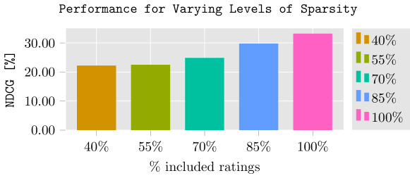
Figure 4. The figure reports the performance of RecWalk on the movielens data, under different sparsity settings. Model selection was performed for each setting following the procedure detailed in Section 6.2 and by considering the hyperparameters: (fixed) $C=200$, (fixed) $\alpha=0.005$, $\gamma_{1}\in\{1,3,5,10\},\gamma_{2}\in\{0.1,0.5,1,3,5,7,9,11,15,20\}$ and $K\in\{3,\dots,20\}$.

We find that RecWalk manages to retain more that 2/3 of its full recommendation accuracy even in the case where only 40% of the available feedback is exploited (specifically, RecWalk’s NDCG@10 on the sparsest case is 33.2% lower than its corresponding performance when all available data are used). Expectedly, as the percentage of included interactions grows, the quality of the trained model improves and the recommendation accuracy increases significantly. Finally, we find that full itemspace coverage is attained for every user in the system even in the sparsest setting.

References

- (1)
- Adomavicius and Tuzhilin (2005) Gediminas Adomavicius and Alexander Tuzhilin. 2005. Toward the next generation of recommender systems: A survey of the state-of-the-art and possible extensions. IEEE Transactions on Knowledge & Data Engineering 6 (2005), 734–749.
- Ando et al. (1963) Albert Ando, Franklin M Fisher, and Herbert Alexander Simon. 1963. Essays on the structure of social science models. Mit Press Cambridge.
- Berberidis et al. (2019) D. Berberidis, A. N. Nikolakopoulos, and G. B. Giannakis. 2019. Adaptive Diffusions for Scalable Learning Over Graphs. IEEE Transactions on Signal Processing 67, 5 (March 2019), 1307–1321. https://doi.org/10.1109/TSP.2018.2889984
- Cevahir et al. (2011) A. Cevahir, C. Aykanat, A. Turk, and B.B. Cambazoglu. 2011. Site-Based Partitioning and Repartitioning Techniques for Parallel PageRank Computation. Parallel and Distributed Systems, IEEE Transactions on 22, 5 (2011), 786–802.
- Christoffel et al. (2015) Fabian Christoffel, Bibek Paudel, Chris Newell, and Abraham Bernstein. 2015. Blockbusters and wallflowers: Accurate, diverse, and scalable recommendations with random walks. In Proceedings of the 9th ACM Conference on Recommender Systems. ACM, 163–170.
- Cooper et al. (2014) Colin Cooper, Sang Hyuk Lee, Tomasz Radzik, and Yiannis Siantos. 2014. Random Walks in Recommender Systems: Exact Computation and Simulations. In Proceedings of the 23rd International Conference on World Wide Web (Seoul, Korea) (WWW ’14 Companion). ACM, New York, NY, USA, 811–816. https://doi.org/10.1145/2567948.2579244
- Courtois (1977) Pierre-Jacque Courtois. 1977. Decomposability: Queueing and Computer System Applications. Academic Press. http://books.google.gr/books?id=jD5RAAAAMAAJ
- Cremonesi et al. (2010) Paolo Cremonesi, Yehuda Koren, and Roberto Turrin. 2010. Performance of recommender algorithms on top-n recommendation tasks. In Proceedings of the fourth ACM conference on Recommender systems (Barcelona, Spain) (RecSys ’10). ACM, 39–46. https://doi.org/10.1145/1864708.1864721
- Deshpande and Karypis (2004) Mukund Deshpande and George Karypis. 2004. Item-based top-N Recommendation Algorithms. ACM Trans. Inf. Syst. 22, 1 (Jan. 2004), 143–177. https://doi.org/10.1145/963770.963776
- Eksombatchai et al. (2018) Chantat Eksombatchai, Pranav Jindal, Jerry Zitao Liu, Yuchen Liu, Rahul Sharma, Charles Sugnet, Mark Ulrich, and Jure Leskovec. 2018. Pixie: A System for Recommending 3+ Billion Items to 200+ Million Users in Real-Time. In Proceedings of the 2018 World Wide Web Conference (Lyon, France) (WWW ’18). International World Wide Web Conferences Steering Committee, Republic and Canton of Geneva, Switzerland, 1775–1784. https://doi.org/10.1145/3178876.3186183
- Feng et al. (2006) Guang Feng, Tie-Yan Liu, Ying Wang, Ying Bao, Zhiming Ma, Xu-Dong Zhang, and Wei-Ying Ma. 2006. AggregateRank: bringing order to web sites. In Proceedings of the 29th annual international ACM SIGIR conference on Research and development in information retrieval (Seattle, Washington, USA) (SIGIR ’06). ACM, New York, NY, USA, 75–82. https://doi.org/10.1145/1148170.1148187
- Fouss et al. (2012) François Fouss, Kevin Francoisse, Luh Yen, Alain Pirotte, and Marco Saerens. 2012. An experimental investigation of kernels on graphs for collaborative recommendation and semisupervised classification. Neural Networks 31 (2012), 53–72.
- Goel et al. (2015) Ashish Goel, Pankaj Gupta, John Sirois, Dong Wang, Aneesh Sharma, and Siva Gurumurthy. 2015. The Who-To-Follow System at Twitter: Strategy, Algorithms, and Revenue Impact. Interfaces 45, 1 (Feb. 2015), 98–107. https://doi.org/10.1287/inte.2014.0784
- Grimmett and Stirzaker (2001) Geoffrey Grimmett and David Stirzaker. 2001. Probability and random processes. Oxford university press.
- He and McAuley (2016) Ruining He and Julian McAuley. 2016. Ups and Downs: Modeling the Visual Evolution of Fashion Trends with One-Class Collaborative Filtering. In Proceedings of the 25th International Conference on World Wide Web (Montréal, Québec, Canada) (WWW ’16). International World Wide Web Conferences Steering Committee, Republic and Canton of Geneva, Switzerland, 507–517. https://doi.org/10.1145/2872427.2883037
- He et al. (2018a) Xiangnan He, Zhankui He, Xiaoyu Du, and Tat-Seng Chua. 2018a. Adversarial Personalized Ranking for Recommendation. In The 41st International ACM SIGIR Conference on Research & Development in Information Retrieval (Ann Arbor, MI, USA) (SIGIR ’18). ACM, New York, NY, USA, 355–364. https://doi.org/10.1145/3209978.3209981
- He et al. (2018b) X. He, Z. He, J. Song, Z. Liu, Y. Jiang, and T. Chua. 2018b. NAIS: Neural Attentive Item Similarity Model for Recommendation. IEEE Transactions on Knowledge and Data Engineering 30, 12 (Dec 2018), 2354–2366. https://doi.org/10.1109/TKDE.2018.2831682
- He et al. (2017) Xiangnan He, Lizi Liao, Hanwang Zhang, Liqiang Nie, Xia Hu, and Tat-Seng Chua. 2017. Neural Collaborative Filtering. In Proceedings of the 26th International Conference on World Wide Web (Perth, Australia) (WWW ’17). International World Wide Web Conferences Steering Committee, Republic and Canton of Geneva, Switzerland, 173–182. https://doi.org/10.1145/3038912.3052569
- Hidasi et al. (2015) Balázs Hidasi, Alexandros Karatzoglou, Linas Baltrunas, and Domonkos Tikk. 2015. Session-based recommendations with recurrent neural networks. arXiv preprint arXiv:1511.06939 (2015).
- Hu et al. (2008) Yifan Hu, Yehuda Koren, and Chris Volinsky. 2008. Collaborative filtering for implicit feedback datasets. In Data Mining, 2008. ICDM’08. Eighth IEEE International Conference on. Ieee, 263–272.
- Kabbur et al. (2013) Santosh Kabbur, Xia Ning, and George Karypis. 2013. FISM: Factored Item Similarity Models for top-N Recommender Systems. In Proceedings of the 19th ACM SIGKDD International Conference on Knowledge Discovery and Data Mining (Chicago, Illinois, USA) (KDD ’13). ACM, New York, NY, USA, 659–667. https://doi.org/10.1145/2487575.2487589
- Kamvar et al. (2003) Sepandar D. Kamvar, Taher H. Haveliwala, Christopher D. Manning, and Gene H. Golub. 2003. Exploiting the Block Structure of the Web for Computing PageRank. In Stanford University Technical Report.
- Kang and McAuley (2018) Wang-Cheng Kang and Julian McAuley. 2018. Self-attentive sequential recommendation. In 2018 IEEE International Conference on Data Mining (ICDM). IEEE, 197–206.
- Kang et al. (2016) Zhao Kang, Chong Peng, Ming Yang, and Qiang Cheng. 2016. Top-n recommendation on graphs. In Proceedings of the 25th ACM International on Conference on Information and Knowledge Management. ACM, 2101–2106.
- Koren (2010) Yehuda Koren. 2010. Factor in the neighbors: Scalable and accurate collaborative filtering. ACM Transactions on Knowledge Discovery from Data (TKDD) 4, 1 (2010), 1.
- Langville and Meyer (2011) Amy N. Langville and Carl D. Meyer. 2011. Google’s PageRank and beyond: The science of search engine rankings. Princeton University Press.
- Liang et al. (2018) Dawen Liang, Rahul G. Krishnan, Matthew D. Hoffman, and Tony Jebara. 2018. Variational Autoencoders for Collaborative Filtering. In Proceedings of the 2018 World Wide Web Conference (Lyon, France), 689–698. https://doi.org/10.1145/3178876.3186150
- Meunier et al. (2010) David Meunier, Renaud Lambiotte, and Edward T Bullmore. 2010. Modular and hierarchically modular organization of brain networks. Frontiers in neuroscience 4 (2010).
- Meyer (2000) Carl D. Meyer. 2000. Matrix analysis and applied linear algebra. Vol. 2. Siam.
- Meyer and Wessell (2012) Carl D. Meyer and Charles D. Wessell. 2012. Stochastic Data Clustering. SIAM J. Matrix Anal. Appl. 33, 4 (2012), 1214–1236.
- Nikolakopoulos and Garofalakis (2013) Athanasios N. Nikolakopoulos and John D. Garofalakis. 2013. NCDawareRank: a novel ranking method that exploits the decomposable structure of the web. In Proceedings of the sixth ACM international conference on Web search and data mining (Rome, Italy) (WSDM ’13). ACM, New York, NY, USA, 143–152. https://doi.org/10.1145/2433396.2433415
- Nikolakopoulos and Garofalakis (2015a) Athanasios N Nikolakopoulos and John D Garofalakis. 2015a. Random surfing without teleportation. In Algorithms, Probability, Networks, and Games. Springer, 344–357.
- Nikolakopoulos and Garofalakis (2015b) Athanasios N. Nikolakopoulos and John D. Garofalakis. 2015b. Top-N recommendations in the presence of sparsity: An NCD-based approach. Web Intelligence 14, 1 (2015), 1–19. https://doi.org/10.3233/WEB-150324
- Nikolakopoulos et al. (2014) Athanasios N Nikolakopoulos, Maria Kalantzi, and John D Garofalakis. 2014. On the use of lanczos vectors for efficient latent factor-based top-n recommendation. In Proceedings of the 4th International Conference on Web Intelligence, Mining and Semantics (WIMS14). ACM, 28.
- Nikolakopoulos et al. (2019) Athanasios N Nikolakopoulos, Vassilis Kalantzis, Efstratios Gallopoulos, and John D Garofalakis. 2019. EigenRec: generalizing PureSVD for effective and efficient top-N recommendations. Knowledge and Information Systems 58, 1 (2019), 59–81.
- Nikolakopoulos and Karypis (2019) Athanasios N. Nikolakopoulos and George Karypis. 2019. RecWalk: Nearly Uncoupled Random Walks for Top-N Recommendation. In Proceedings of the Twelfth ACM International Conference on Web Search and Data Mining (Melbourne, Australia) (WSDM ’19). ACM, New York, NY, USA, 9. https://doi.org/10.1145/3289600.3291016
- Nikolakopoulos et al. (2016) A. N. Nikolakopoulos, A. Korba, and J. D. Garofalakis. 2016. Random surfing on multipartite graphs. In 2016 IEEE International Conference on Big Data (Big Data). 736–745. https://doi.org/10.1109/BigData.2016.7840666
- Nikolakopoulos et al. (2013) Athanasios N Nikolakopoulos, Marianna Kouneli, and John Garofalakis. 2013. A novel hierarchical approach to ranking-based collaborative filtering. In International Conference on Engineering Applications of Neural Networks. Springer, 50–59.
- Nikolakopoulos et al. (2015) Athanasios N. Nikolakopoulos, Marianna A. Kouneli, and John Garofalakis. 2015. Hierarchical Itemspace Rank: Exploiting hierarchy to alleviate sparsity in ranking-based recommendation. Neurocomputing 163 (2015), 126–136. https://doi.org/10.1016/j.neucom.2014.09.082
- Ning et al. (2015) Xia Ning, Christian Desrosiers, and George Karypis. 2015. A comprehensive survey of neighborhood-based recommendation methods. In Recommender systems handbook. Springer, 37–76.
- Ning and Karypis (2011) Xia Ning and George Karypis. 2011. Slim: Sparse linear methods for top-n recommender systems. In 2011 11th IEEE International Conference on Data Mining. IEEE, 497–506.
- Ning and Karypis (2012) Xia Ning and George Karypis. 2012. Sparse linear methods with side information for top-n recommendations. In Proceedings of the sixth ACM conference on Recommender systems. ACM, 155–162.
- Ning et al. (2019) Xia Ning, Athanasios N. Nikolakopoulos, Zeren Shui, Mohit Sharma, and George Karypis. 2019. SLIM Library for Recommender Systems. https://github.com/KarypisLab/SLIM
- Page et al. (1999) Lawrence Page, Sergey Brin, Rajeev Motwani, and Terry Winograd. 1999. The PageRank Citation Ranking: Bringing Order to the Web. Technical Report 1999-66. Stanford InfoLab. http://ilpubs.stanford.edu:8090/422/
- Reinstaller (2007) Andreas Reinstaller. 2007. The division of labor in the firm: Agency, near-decomposability and the Babbage principle. Journal of Institutional Economics 3 (12 2007), 293–322. Issue 03. https://doi.org/10.1017/S1744137407000732
- Rendle et al. (2009) Steffen Rendle, Christoph Freudenthaler, Zeno Gantner, and Lars Schmidt-Thieme. 2009. BPR: Bayesian personalized ranking from implicit feedback. In Proceedings of the twenty-fifth conference on uncertainty in artificial intelligence. AUAI Press, 452–461.
- Sarasvathy (2003) Saras D Sarasvathy. 2003. Entrepreneurship as a science of the artificial. Journal of Economic Psychology 24, 2 (2003), 203 – 220. https://doi.org/10.1016/S0167-4870(02)00203-9 The Economic Psychology of Herbert A. Simon.
- Sarwar et al. (2001) Badrul Sarwar, George Karypis, Joseph Konstan, and John Riedl. 2001. Item-based collaborative filtering recommendation algorithms. In Proceedings of the 10th international conference on World Wide Web. ACM, 285–295.
- Shpak et al. (2004) Max Shpak, Peter Stadler, Gunter P Wagner, and Lee Altenberg. 2004. Simon-Ando decomposability and fitness landscapes. Theory in Biosciences 123, 2 (2004), 139–180.
- Simon and Ando (1961) Herbert A. Simon and Albert Ando. 1961. Aggregation of variables in dynamic systems. Econometrica: Journal of The Econometric Society (1961), 111–138.
- Steck (2019) Harald Steck. 2019. Embarrassingly Shallow Autoencoders for Sparse Data. In The World Wide Web Conference (San Francisco, CA, USA) (WWW ’19). ACM, New York, NY, USA, 3251–3257. https://doi.org/10.1145/3308558.3313710
- Stewart (1991) GW Stewart. 1991. On the sensitivity of nearly uncoupled Markov chains. Numerical solution of Markov chains. Probability: pure and applied 8 (1991), 105–119.
- Stewart (1994) William J. Stewart. 1994. Introduction to the numerical solution of Markov chains. Princeton University Press.
- Tang and Wang (2018) Jiaxi Tang and Ke Wang. 2018. Personalized top-n sequential recommendation via convolutional sequence embedding. In Proceedings of the Eleventh ACM International Conference on Web Search and Data Mining. ACM, 565–573.
- Weston et al. (2013) Jason Weston, Ron J Weiss, and Hector Yee. 2013. Nonlinear latent factorization by embedding multiple user interests. In Proceedings of the 7th ACM conference on Recommender systems. ACM, 65–68.
- Wu et al. (2016) Yao Wu, Christopher DuBois, Alice X Zheng, and Martin Ester. 2016. Collaborative denoising auto-encoders for top-n recommender systems. In Proceedings of the Ninth ACM International Conference on Web Search and Data Mining. ACM, 153–162.
- Xue et al. (2018) Feng Xue, Xiangnan He, Xiang Wang, Jiandong Xu, Kai Liu, and Richang Hong. 2018. Deep Item-based Collaborative Filtering for Top-N Recommendation. arXiv preprint arXiv:1811.04392 (2018).
- Yakob and Tell (2007) Ramsin Yakob and Fredrik Tell. 2007. Managing near decomposability in complex platform development projects. International Journal of Technology Intelligence and Planning 3, 4 (2007), 387–407.
- Yayavaram and Ahuja (2008) Sai Yayavaram and Gautam Ahuja. 2008. Decomposability in knowledge structures and its impact on the usefulness of inventions and knowledge-base malleability. Administrative Science Quarterly 53, 2 (2008), 333–362.
- Zhang et al. (2019) Shuai Zhang, Lina Yao, Aixin Sun, and Yi Tay. 2019. Deep learning based recommender system: A survey and new perspectives. ACM Computing Surveys (CSUR) 52, 1 (2019), 5.
- Zheng et al. (2014) Yong Zheng, Bamshad Mobasher, and Robin Burke. 2014. CSLIM: Contextual SLIM recommendation algorithms. In Proceedings of the 8th ACM Conference on Recommender Systems. ACM, 301–304.
- Zhou et al. (2010) Tao Zhou, Zoltán Kuscsik, Jian-Guo Liu, Matúš Medo, Joseph Rushton Wakeling, and Yi-Cheng Zhang. 2010. Solving the apparent diversity-accuracy dilemma of recommender systems. Proceedings of the National Academy of Sciences 107, 10 (2010), 4511–4515. https://doi.org/10.1073/pnas.1000488107 arXiv:https://www.pnas.org/content/107/10/4511.full.pdf
- Zhu et al. (2005) Yangbo Zhu, Shaozhi Ye, and Xing Li. 2005. Distributed PageRank computation based on iterative aggregation-disaggregation methods. In Proceedings of the 14th ACM international conference on Information and knowledge management. ACM, 578–585.