Role of the confinement-induced effective range on the thermodynamics of a strongly correlated Fermi gas in two dimensions

Abstract

We theoretically investigate the thermodynamic properties of a strongly correlated two-dimensional Fermi gas with a confinement-induced negative effective range of interactions, which is described by a two-channel model Hamiltonian. By extending the many-body $T$-matrix approach by Nozières and Schmitt-Rink to the two-channel model, we calculate the equation of state in the normal phase and present several thermodynamic quantities as functions of temperature, interaction strength, and effective range. We find that there is a non-trivial dependence of thermodynamics on the effective range. In experiment, where the effective range is set by the tight axial confinement, the contribution of the effective range becomes non-negligible as the temperature decreases down to the degenerate temperature. We compare our finite-range results with recent measurements on the density equation of state, and show that the effective range has to be taken into account for the purpose of a quantitative understanding of the experimental data.

I Introduction

Recent developments in creating ultracold atomic gases in lower dimensions has opened up a new and exciting field to explore strongly correlated many-body systems Levinsen2015 ; Turlapov2017 . Two-dimensional (2D) ultracold atomic Fermi gases are of interest due to the increased role of thermal and quantum fluctuations, which lead to, for example, suppressed superfluid long-range order at nonzero temperature and a quasi-ordered transition to superfluidity, the Berezinksii-Kosterlitz-Thouless (BKT) transition Berezinski1972 ; Kosterlitz1973 . In addition to presenting a range of novel and intriguing quantum phenomena, such as scale invariance and the breathing mode anomaly Holstein1993 ; Pitaevskii1997 ; Olshanii2010 ; Hofmann2012 ; Taylor2012 and novel topological phases Liu2012 ; Cao2014 ; Goldman2016 , 2D Fermi gases provide an important tool in understanding confined many-body systems from diverse fields of physics, such as: high-temperature superconductors Loktev2001 , thin ³He films Ruggeri2013 , neutron stars in a nuclear pasta phase Pons2013 , and exciton-polariton condensates in a microcavity Deng2010 .

The key advantage of 2D ultracold Fermi gases is their unprecedented controllability: the interatomic interaction can be tuned continuously with Feshbach resonances to realize the crossover from a Bardeen-Cooper-Scrieffer (BCS) superfluid of weakly interacting Cooper pairs to a Bose-Einstein condensate (BEC) of tightly bound molecules Turlapov2017 ; Makhalov2014 , the population of spin components can be changed Feld2011 , the confining potential can be made homogeneous with a box potential Hueck2018 , and non-abelian synthetic gauge field (i.e. spin-orbit coupling) can be devised Zhang2014 .

With these advancements, a set of seminal experiments directly probed the universal thermodynamics of a 2D interacting Fermi gas at given interaction strengths Makhalov2014 ; Martiyanov2016 ; Fenech2016 ; Boettcher2016 , by measuring the in-trap density profile. This allows for a direct comparison between theoretical predictions and experimental data. To date, it has been found that, a single-channel model with a single 2D $s$-wave scattering length works reasonably well in describing the equation of state (EoS) experimental results, both in the normal state Watanabe2013 ; Bauer2014 ; Barth2014 ; Anderson2015 ; Mulkerin2015 and below the BKT transition Bertaina2012 ; He2015 ; Shi2015 ; Mulkerin2017 . However, in the strongly correlated regime it turns out that, the theoretical EoS determined by accurate auxiliary-field quantum Monte Carlo (AFQMC) simulations Shi2015 slightly over-estimates the thermodynamics compared to the measured EoS Turlapov2017 ; Makhalov2014 ; Martiyanov2016 , suggesting the inefficiency of the single-channel model. The necessity of using a more appropriate theoretical model was highlighted by the most recent measurements on the breathing mode Vogt2012 ; Holten2018 ; Peppler2018 , which present an interesting example of a quantum anomaly (i.e., violation of the classical scale invariance Pitaevskii1997 ). It was found that the measured breathing mode is notably lower than the prediction from the single-channel model Hofmann2012 ; Taylor2012 . This discrepancy can not be fully understood by the nonzero but small temperature found in the experiments Mulkerin2018 . Instead, it is caused by a confinement-induced effective range of interactions, which is negative and turns out be significant under the current experimental conditions Hu2019 . By adopting a two-channel model to account for the effective range, both measurements on low-temperature EoS and breathing mode anomaly can now be satisfactorily explained by calculations at zero temperature Wu2019 .

In this work, we explore how the confinement-induced effective range changes the finite-temperature thermodynamic properties of a normal, strongly-correlated 2D Fermi gas. Our purpose is two-fold. First, characterizing the thermodynamics of the normal state of strongly correlated Fermi gases may be relevant to understanding the role of many-body pairing Murthy2018 , which is a precursor to superfluidity Watanabe2013 . The results presented here can be used to better understand the existing two experimental measurements of the EoS at finite temperature in the normal phase Fenech2016 ; Boettcher2016 . Through the simplest many-body $T$-matrix theory developed by Nozières and Schmidt-Rink (NSR) Nozieres1985 , we determine the thermodynamic potential of the two-channel model, and calculate how the pressure EoS, energy, and entropy change with a negative effective range. Second, we then consider the realistic effective range in two recent experiments Fenech2016 ; Boettcher2016 and compare our finite-range results with experimental data on density EoS. We find that in the experiments the effect of the effective range starts to show up when the temperature is decreased down to Fermi degeneracy. To quantitatively explain the experimental density EoS at finite temperature near superfluid transition, therefore, the effective range has to be taken into account in future refined theoretical works.

We note that, for a three-dimensional (3D) interacting Fermi gas, the effect of a negative effective range has been recently discussed by Tajima Tajima2018 ; Tajima2019 , following the seminal work by Ohashi and Griffin Ohashi2003 , who extended the NSR approach to the two-channel model. There, the effective range is related to the width of Feshbach resonance and the 3D interacting Fermi gas may experience severe atom loss in the narrow resonance limit (i.e., at a large negative effective range) Hazlett2012 . In our case, the confinement-induced effective range is intrinsically set by the tight axial confinement and the 2D interacting Fermi gas is always mechanically stable.

Our manuscript is set out as follows. In Sec. II, we introduce the two-channel model Hamiltonian and renormalize the relevant parameters by solving the two-body scattering problem. In Sec. III, we briefly outline the many-body effective field theory of the model Hamiltonian and show how to calculate the thermodynamic observables. In Sec. IV, we discuss the thermodynamic properties of the 2D interacting Fermi gas, as functions of the effective range, temperature and interaction strength. And finally in Sec. V, we summarize our results. For simplicity we set $\hbar=1$ throughout.

II Hamiltonian and two-particle scattering

We begin our calculation of the thermodynamic properties by considering a two-component Fermi gas in the normal state, described by the two-channel Hamiltonian Tajima2018 ; Tajima2019 ; Ohashi2003 ; Liu2005 ; Schonenberg2017 :

$$\mathcal{H} = \sum_{\mathbf{k}\sigma}\xi_{\mathbf{k}}c_{\mathbf{k}\sigma}^{\dagger}c_{\mathbf{k}\sigma}^{\phantom{\dagger}}+\sum_{\mathbf{q}}\left(\epsilon_{\mathbf{q}}/2+\nu-2\mu\right)b_{\mathbf{q}}^{\dagger}b_{\mathbf{q}}^{\phantom{\dagger}}$$ (1)

$$+g\sum_{kq}\left(b_{\mathbf{q}}^{\phantom{\dagger}}c_{\mathbf{q}/2+\mathbf{k}\uparrow}^{\dagger}c_{\mathbf{q}/2-\mathbf{k}\downarrow}^{\dagger}+{\rm H.c.}\right),$$

where ${\rm H.c.}$ is the Hermitian conjugate, $c_{\mathbf{k}\sigma}$ are the annihilation operators of fermionic atoms with spin $\sigma=\uparrow,\downarrow$ and mass $M$ in the open channel, and $b_{\mathbf{q}}$ the annihilation operators of bosonic molecules in the closed channel. The kinetic energy of atoms measured from the chemical potential $\mu$ is $\xi_{\mathbf{k}}=\epsilon_{\mathbf{k}}-\mu$, where $\epsilon_{\mathbf{k}}=\mathbf{k}^{2}/(2M)$. The threshold energy or detuning of the diatomic molecules is $\nu$ and the Feshbach coupling between atoms and molecules is given by $g$.

In order to find the many-body properties we require the bare two-body scattering parameters to be rewritten in terms of measurable or renormalizable scattering parameters. To relate the detuning $\nu$ and the channel coupling $g$ to physical observables, we consider the two-body $T$-matrix in a vacuum ($E^{+}\equiv k^{2}/M+i0^{+}$) Hu2019 ; Liu2005 ,

$$T_{2B}^{-1}\left(E^{+}\right)=U_{\textrm{eff}}^{-1}+\sum_{\mathbf{p}}\frac{1}{2\epsilon_{\mathbf{p}}-E^{+}},$$ (2)

where the effective interaction in the presence of the channel coupling is given by

$$U_{\textrm{eff}}\left(E^{+}\right)=\frac{g^{2}}{E^{+}-\nu}.$$ (3)

Taking a large momentum cut-off, $\Lambda\rightarrow\infty$, we write the two-body $T$-matrix as

$$T_{2B}^{-1}\left(E^{+}\right)=\frac{k^{2}/M-\nu}{g^{2}}+\frac{M}{4\pi}\left(\ln\left[\frac{\Lambda^{2}}{k^{2}}-1\right]+i\pi\right).$$ (4)

Alternatively, we may rewrite it in the form,

$$T_{2B}\left(E^{+}\right)=\frac{m}{4\pi}\left(-2\ln\left[ka_{s}\right]-R_{s}k^{2}+i\pi\right),$$ (5)

where we have written the detuning and Feshbach coupling in terms of the 2D scattering length $a_{s}$ and effective range $R_{s}$ Schonenberg2017 ,

$$a_{s}=\frac{1}{\Lambda}e^{\frac{2\pi\nu}{gM}},\;\;R_{s}=-\frac{4\pi}{M^{2}}\frac{1}{g^{2}}.$$ (6)

As can be seen from Eq. (6), we recover the single-channel model in the broad resonance limit when $g\rightarrow\infty$. We may remove the cut-off $\Lambda$ by considering the pole of the two-body $T$-matrix $T_{2B}(E)$, $E=E_{B}$. We find that,

$$\nu=E_{B}+g^{2}\sum_{\mathbf{k}}\frac{1}{2\epsilon_{\mathbf{k}}-E_{B}}.$$ (7)

The binding energy can be set by $\varepsilon_{B}=-E_{B}=\kappa^{2}/M$, where $k=i\kappa$ corresponds to the pole of the two-body $T$-matrix.

III The many-body $T$-matrix

We consider the strong-coupling effects and pairing fluctuations by applying the normal-state NSR approach Nozieres1985 , which has been widely used in different context and has also been extended to superfluid phase He2015 ; Hu2006 ; Hu2007 ; Diener2008 . For completeness, here we briefly go through the derivation of the thermodynamic potential using the functional path-integral formalism. All the thermodynamic properties can be obtained through the thermodynamic potential, $\Omega=-k_{B}T\ln\mathcal{Z}$, where the partition function $\mathcal{Z}$ for the two-channel Hamiltonian is given by,

$$\mathcal{Z}=\int\mathcal{D}\left(c^{\,},c^{\dagger}\right)\mathcal{D}\left(b^{\,},b^{\dagger}\right)e^{-\mathcal{S}\left[c^{\,},c^{\dagger},b^{\,},b^{\dagger}\right]},$$ (8)

for atomic fields $(c_{\mathbf{k}\sigma}^{\phantom{\dagger}},\,c_{\mathbf{k}\sigma}^{\dagger})$ and molecular fields $(b_{\mathbf{q}}^{\phantom{\dagger}},\,b_{\mathbf{q}}^{\dagger})$, and the action at the inverse temperature $\beta=1/(k_{B}T)$ is given by,

$$\mathcal{S}=\int_{0}^{\beta}d\tau \biggl{[}\sum_{\mathbf{k}\sigma}c_{\mathbf{k}\sigma}^{\dagger}(\tau)c_{\mathbf{k}\sigma}^{\,}(\tau)$$

$$+\sum_{\mathbf{q}}b_{\mathbf{q}}^{\dagger}(\tau)\partial_{\tau}b_{\mathbf{q}}^{\,}(\tau)+\mathcal{H}(\tau)\biggl{]}.$$ (9)

Using the Hubbard-Stratonovich transformation to decouple the Feshbach coupling term and integrating out the atomic fields, we obtain an effective action for Cooper pairs and molecules. By further truncating the perturbative expansion over bosonic fields (for both pairs and molecules) at the Gaussian fluctuation level, we arrive at the NSR thermodynamic potential Ohashi2003 ,

$$\Omega=\Omega_{{\rm F}}+\Omega_{{\rm B}}-\sum_{\mathbf{q},i\nu_{n}}\ln\left[1+g^{2}D_{0}(\mathbf{q},i\nu_{n})\Pi(\mathbf{q},i\nu_{n})\right],$$ (10)

where $\nu_{n}=2n\pi/\beta$ are the bosonic Matsubara frequencies, $\Omega_{{\rm F}}=2\sum_{\mathbf{k}}\ln(e^{-\beta\xi_{\mathbf{k}}}+1)$ and $\Omega_{{\rm B}}=\sum_{\mathbf{q}}\ln(e^{-\beta\epsilon_{\mathbf{q}}^{{\rm B}}}-1)$ are the free fermionic and bosonic thermodynamic potentials for atoms and molecules, respectively. We have defined the pair correlation function

$$\Pi(\mathbf{q},i\nu_{n})=\sum_{\mathbf{k}}\frac{1-f(\xi_{\frac{\mathbf{q}}{2}-\mathbf{k}})-f(\xi_{\frac{\mathbf{q}}{2}+\mathbf{k}})}{2\epsilon_{\mathbf{k}}-2\mu+\epsilon_{\mathbf{q}}/2-i\nu_{n}},$$ (11)

and $D_{0}(\mathbf{q},i\nu_{m})=1/(i\nu_{n}-\epsilon_{\mathbf{q}}^{{\rm B}})$ is the Green’s function of a free molecular boson with dispersion $\epsilon_{\mathbf{q}}^{{\rm B}}=\mathbf{q}/2-\nu+2\mu$. The thermodynamic potential can be rewritten into the following form:

$$\Omega=\Omega_{{\rm F}}-\sum_{\mathbf{q},i\nu_{n}}\ln\left[-\Gamma^{-1}(\mathbf{q},i\nu_{n})\right],$$ (12)

where we have introduced the vertex function

$$\Gamma^{-1}(\mathbf{q},i\nu_{n})=U_{{\rm eff}}^{-1}\left(\mathbf{q},i\nu_{m}\right)+\Pi\left(\mathbf{q},i\nu_{m}\right),$$ (13)

and the in-medium effective interaction $U_{{\rm eff}}(\mathbf{q},i\nu_{m})\equiv g^{2}D_{0}(\mathbf{q},i\nu_{m})$, which can be explicitly written as,

$$\frac{1}{U_{{\rm eff}}\left(\mathbf{q},i\nu_{m}\right)} = -\sum_{\mathbf{k}}\frac{1}{2\epsilon_{\mathbf{k}}+\varepsilon_{B}}-$$ (14)

$$\frac{M^{2}R_{s}}{4\pi}\left(i\nu_{n}-\frac{\epsilon_{\mathbf{q}}}{2}+2\mu+\varepsilon_{B}\right).$$

Using Eq. (14) we cancel off the divergent parts in $\Pi(\mathbf{q},i\nu_{n})$. Analytically continuing the vertex function, $i\nu_{n}\rightarrow\omega+i0^{+}$, we calculate the thermodynamic potential:

$$\Omega=\Omega_{\textrm{F}}-\frac{1}{\pi}\sum_{\mathbf{q}}\int_{-\infty}^{\infty}\frac{d\omega}{e^{\beta\omega}-1}\delta(\mathbf{q},\omega),$$ (15)

where $\delta(\mathbf{q},\omega)\equiv-{\rm Im}\ln[-\Gamma^{-1}(\mathbf{q},\omega+i0^{+})]$ is the phase of the vertex function. The number equation $nV=N=-d\Omega/d\mu$, where $N$ is the total number of atoms and molecules and $V$ is the area (or the volume in 2D), is solved to yield the chemical potential $\mu$ at a given set of reduced temperature $T/T_{{\rm F}}$, binding energy $\varepsilon_{B}/E_{{\rm F}}$, and effective range $k_{{\rm F}}^{2}R_{s}$. Here, we define $k_{\textrm{F}}=(2\pi n)^{1/2}$, $E_{\textrm{F}}=k_{\textrm{F}}^{2}/(2M)$, and $T_{\textrm{F}}=E_{\textrm{F}}/k_{B}$.

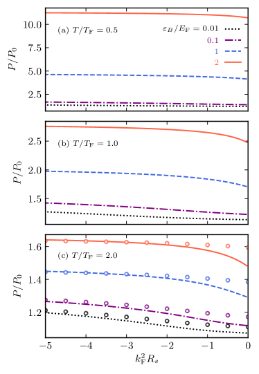
Figure 1: Pressure EoS, normalized by the ideal pressure $P_{0}$ at the same temperature, is plotted as a function of the effective range for interaction strengths $\varepsilon_{B}/E_{{\rm F}}=0.01$ (black-dotted), $\varepsilon_{B}/E_{{\rm F}}=0.1$ (purple-dot dashed), $\varepsilon_{B}/E_{{\rm F}}=1$ (blue-dashed), and $\varepsilon_{B}/E_{{\rm F}}=2$ (red-solid), at temperatures (a) $T/T_{{\rm F}}=0.5$, (b) $T/T_{{\rm F}}=1$, and (c) $T/T_{{\rm F}}=2$. At high temperature in (c), the second order virial expansion results for each interaction strength are shown by circles.

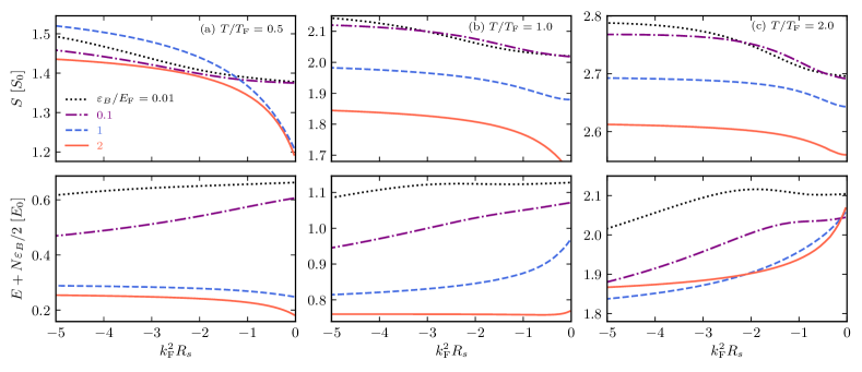
Figure 2: Upper panels: Entropy normalized by $S_{0}=k_{B}N$ as a function of the effective range at different interaction strengths $\varepsilon_{B}/E_{{\rm F}}=0.01$ (black-dotted), $\varepsilon_{B}/E_{{\rm F}}=0.1$ (purple-dot dashed), $\varepsilon_{B}/E_{{\rm F}}=1$ (blue-dashed), and $\varepsilon_{B}/E_{{\rm F}}=2$ (red-solid). The columns (a), (b), and (c) are for temperatures $T/T_{{\rm F}}=0.5$, $T/T_{{\rm F}}=1$, and $T/T_{{\rm F}}=2$, respectively. Lower panels: The effective range dependence of the energy, in units of $E_{0}=NE_{{\rm F}}$, with the same convention as in the upper panels.

We note that within the many-body $T$-matrix framework, we cannot calculate the superfluid transition temperature, i.e. the BKT transition temperature. This is due to the fact that the Thouless criterion in two dimensions becomes inapplicable as a direct consequence of Hohenberg’s theorem and the loss of long-range order due to quantum fluctuations Loktev2001 ; Hohenberg1967 . The self-consistent calculation of the chemical potential and Thouless criterion always leads to a zero critical temperature. To consider the BKT transition the superfluid density needs to be calculated for the two-channel model in the superfluid phase, following the work in Ref. Mulkerin2017 . Such a scheme is beyond the scope of this work.

To calculate the thermodynamic properties of the entropy and energy, we define the dimensionless pressure equation of state $f_{p}$,

$$\frac{P\lambda_{T}^{2}}{k_{{\rm B}}T} \equiv f_{p}\left(x=\frac{T}{T_{{\rm F}}},y=\frac{\varepsilon_{B}}{E_{{\rm F}}},z=k_{{\rm F}}^{2}R_{s}\right),$$ (16)

where the thermal wavelength is $\lambda_{T}=\sqrt{2\pi/(mk_{B}T)}$. All the other thermodynamic observables can then be calculated as derivatives from the dimensionless pressure equation of state, Eq. (16). The entropy is given by

$$S=-\left(\frac{\partial\Omega}{\partial T}\right)_{\mu}\equiv Nk_{B}f_{s},$$ (17)

where the dimensionless entropy takes the form,

$$f_{s}=2f_{p}-\frac{\tilde{\mu}}{x}f_{p_{x}}-\frac{k_{B}y}{x}f_{p_{y}},$$ (18)

and $f_{p_{x}}\equiv\partial f_{p}/\partial x$, and $\tilde{\mu}=\mu/E_{{\rm F}}$. The energy is found through $E=-TS+\Omega+\mu N\equiv NE_{{\rm F}}f_{E}$, and we obtain

$$f_{E}=xf_{s}+x\frac{f_{p}}{f_{p_{x}}}+\tilde{\mu}.$$ (19)

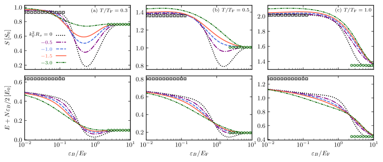
Figure 3: Upper panels: Entropy is plotted in units of $S_{0}=Nk_{{\rm B}}$ as a function of the interaction strength at different negative effective ranges: $k_{{\rm F}}^{2}R_{s}=0$ (black dotted), $k_{{\rm F}}^{2}R_{s}=-0.5$ (purple dot-dashed), $k_{{\rm F}}^{2}R_{s}=-1$ (blue dashed), $k_{{\rm F}}^{2}R_{s}=-1.5$ (red solid), and $k_{{\rm F}}^{2}R_{s}=-3$ (green dot-dot-dashed), for temperatures (a) $T/T_{{\rm F}}=0.3$, (b) $T/T_{{\rm F}}=0.5$, and (c) $T/T_{{\rm F}}=1.0$. The square and circular symbols are the ideal Fermi and Bose gas limits (see text), respectively. Lower panels: Energy is plotted in units of $E_{0}=NE_{{\rm F}}$. The same convention was taken as in the upper panels.

IV Results and discussions

IV.1 Pressure equation of state

To begin our analysis of the thermodynamic properties of the system, we plot the pressure EoS in Fig. 1, which is normalized with the pressure of an ideal Fermi gas at the same temperature, $P_{0}=-2\pi\lambda_{T}^{-4}{\rm Li}_{2}\left(-e^{\beta\mu}\right)$, where ${\rm Li}_{s}(z)$ is the polylogarithm function. We show the pressure EoS at temperatures (a) $T/T_{{\rm F}}=0.5$, (b) $T/T_{{\rm F}}=1$, (c) and $T/T_{{\rm F}}=2$, for a range of interaction strengths, from $\varepsilon_{B}/E_{{\rm F}}=0.01$ to $\varepsilon_{B}/E_{{\rm F}}=2$. We find that, as the effective range decreases, the normalized pressure EoS increases for all temperatures and interaction strengths. This general trend is anticipated, as the system becomes less correlated with increasing effect range. In the limit of infinitely large effective range, $R_{s}\rightarrow\infty$ and $g\rightarrow 0$, the system simply reduces to a non-interacting mixture of atoms and molecules.

As a comparison in the high temperature regime, we consider the virial expansion up to second order Barth2014 ; Liu2010 ; Liu2013 ; Ngampruetikorn2015 ,

$$f_{p}=\int_{0}^{\infty}dt\ln\left[1+ze^{-t}\right]+\Delta b_{2}z^{2}+\dots.,$$ (20)

where $\Delta b_{2}$ is the second-order virial coefficient. By using the elegant Beth-Uhlenbeck relation Beth1937 , we obtain

$$\Delta b_{2}=e^{\beta\varepsilon_{B}}-\int_{0}^{\infty}\frac{dk}{k}e^{-2k^{2}}\frac{2k^{2}R_{s}+2}{\left(\ln\left[\frac{2k^{2}}{\varepsilon_{B}}\right]+k^{2}R_{s}\right)^{2}+\pi^{2}},$$ (21)

which in the zero-range limit reduces to the known results Bauer2014 ; Fenech2016 .

As shown in Fig. 1(c) at a large temperature $T=2T_{\textrm{F}}$, we find that as the effective range decreases, the virial expansion provides an excellent description of the pressure EoS, even for the largest binding energy. This is quite different from the zero-range limit. At $k_{{\rm F}}^{2}R_{s}=0$, where the single-channel model is applicable, the virial expansion systematically overestimates the pressure EoS. The improved applicability of virial expansion is again due to the weaker correlation at nonzero effective range.

IV.2 Entropy and energy

Having discussed the pressure EoS, we now consider the entropy per particle $S/(Nk_{B})$, as shown in the upper panels of Fig. 2 as a function of the negative effective range at three different temperatures, (a) $T/T_{{\rm F}}=0.5$, (b) $T/T_{{\rm F}}=1.0$, and (c) $T/T_{{\rm F}}=2.0$, for a range of binding energies. We find that the entropy has a consistent behavior for all interaction strengths and temperatures: the entropy increases as the effective range decreases. In particular, at low temperature as the negative effective range decreases, we see for large binding energies (i.e., $\varepsilon_{B}/E_{{\rm F}}=1$, $2$) the entropy increases rapidly. This shows that the low-temperature entropy is more sensitive to the effective range than the pressure EoS in the strongly interacting regime.

In the lower panels of Fig. 2, we plot the energy per particle, $E/(NE_{{\rm F}})$, with the two-body contribution from pairs (where we have assumed that there are $N/2$ pairs each with energy $-\varepsilon_{B}$) subtracted. For the weakest binding energy (i.e., in the BCS regime), the energy decreases as the effective range decreases, for all temperatures. However, for larger binding energies at the crossover regime ($\varepsilon_{B}/E_{{\rm F}}=1,\,2$), the energy increases at low temperature with decreasing effective range; while at higher temperatures the energy decreases. The different effective-range dependence of the energy at low and high temperatures may be understood from the many-body pairing. In the low temperature regime for large binding energy, the many-body pairing is important and the system becomes rigid with respect to the change of the effective range. Hence, the energy slightly increases, similar to the pressure EoS. In contrast, at high temperature the many-body pairing is less significant and the system experiences a character change from atoms to molecules with increasing effective range. The energy then decreases, roughly following the picture of a non-interacting Bose and Fermi mixture.

To see the interaction effects on the thermodynamic properties, we show in Fig. 3 the dimensionless entropy (upper panels) and energy (lower panels) as a function of the binding energy, $\varepsilon_{B}/E_{{\rm F}}$, for a range of negative effective ranges from $k_{{\rm F}}^{2}R_{s}=0$ to $-3$ at temperatures (a) $T/T_{{\rm F}}=0.3$, (b) $T/T_{{\rm F}}=0.5$, and (c) $T/T_{{\rm F}}=1.0$. For comparison, we show also the ideal gas limits of Fermi and Bose gases for the entropy and energy. For the ideal Fermi gas limit, we use the following formulas:

$$\frac{S^{{\rm F}}}{Nk_{{\rm B}}} =\frac{2{\rm Li}_{2}\left(-e^{\mu/E_{{\rm F}}}\right)}{{\rm Li}_{1}\left(-e^{\mu/E_{{\rm F}}}\right)}-\frac{\mu}{E_{{\rm F}}},$$ (22)

$$\frac{E^{{\rm F}}}{NE_{{\rm F}}} =-\left(\frac{T}{T_{{\rm F}}}\right)^{2}{\rm Li}_{2}\left(-e^{\mu/E_{{\rm F}}}\right),$$ (23)

with a non-interacting chemical potential $\mu$ determined by using the number equation. To find the entropy and energy for non-interacting Bose gases, $S^{{\rm B}}$ and $E^{{\rm B}}$, we assume a gas of $N/2$ non-interacting molecules with mass $2M$ and similarly solve a molecular chemical potential.

The behavior of the entropy as a function of the binding energy is non-trivial. We find that for $k_{{\rm F}}^{2}R_{s}=0$, as the interaction is increased from the weakly to strongly attractive regimes, the entropy has a local minimum at $\varepsilon_{B}/E_{{\rm F}}\simeq 0.6$ for temperature $T/T_{{\rm F}}=0.3$, $\varepsilon_{B}/E_{{\rm F}}\simeq 1.05$ for temperature $T/T_{{\rm F}}=0.5$, and $\varepsilon_{B}/E_{{\rm F}}\simeq 5$ for temperature $T/T_{{\rm F}}=1.0$. This minimum may be understood as the position where pair formation is the strongest, and at low temperature where there is a defined Fermi surface, i.e., $\mu>0$ for $\varepsilon_{B}/E_{{\rm F}}\lesssim 1$, this pairing is dominated by many-body pairing. As the negative effective range decreases, we see this clear minimum in the crossover interaction regime becomes shallower. For $T/T_{{\rm F}}=0.3$ the minimum shifts to weaker binding energies with decreasing effective range, and for higher temperatures the minimum shifts to larger binding energies and disappears for $k_{{\rm F}}^{2}R_{s}<-1$. In the weakly attractive regime the entropy quickly approaches the non-interacting 2D Fermi gas limit and in the strongly attractive regime the entropy approaches the limit of $N/2$ non-interacting molecules with mass $2M$.

The behavior of the energy is qualitatively the same as the entropy, with a local minimum that shifts to larger binding energy as the temperature increases. We find also that the minimum in the crossover interaction regime becomes much weaker as the negative effective range decreases. Unlike the entropy, the energy is slowly approaching the non-interacting 2D Fermi gas in the weakly attractive regime. However, in the strongly attractive regime the energy quickly approaches the limit of $N/2$ non-interacting molecules.

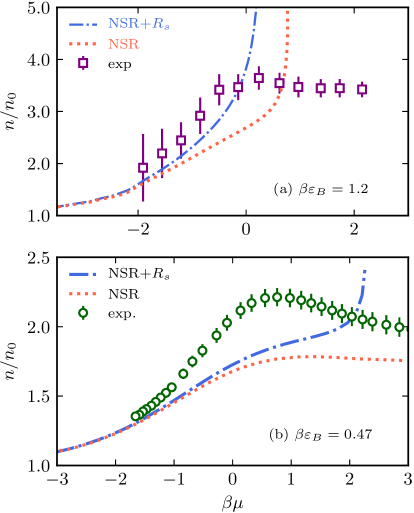
Figure 4: (a) Density EoS, normalized by $n_{0}=-\lambda_{T}^{-2}{\rm Li}_{1}\left(-e^{\beta\mu}\right)$, as a function of the dimensionless chemical potential $\beta\mu$ and interaction strength $\beta\varepsilon_{B}=1.2$, for the single-channel model (red-dotted, $R_{s}=0$), the two-channel model (blue dot-dashed, $R_{s}\neq 0$), and the experimental results from Ref. Boettcher2016 . (b) Density EoS at $\beta\varepsilon_{B}=0.47$, with the experimental results from Ref. Fenech2016 .

IV.3 Comparison to experiment

We now compare our two-channel results to the experimental data on density EoS, with a realistic confinement-induced effective range. For this purpose, we match the the low-energy expansion of $T_{2B}(E^{+}\equiv k^{2}/M+i0^{+})$ to the quasi-2D scattering amplitude $f_{Q2D}(k)/M$, which describes the two-particle scattering within the ground-state manifold under a tight axial confinement with frequency $\omega_{z}$ Petrov2001 :

$$f_{Q2D}(k\rightarrow 0)=\frac{4\pi}{\sqrt{2\pi}a_{z}/a_{3D}+\varpi\left(k^{2}a_{z}^{2}/2\right)},$$ (24)

where $a_{z}\equiv\sqrt{1/(M\omega_{z})}$ is the harmonic oscillator length and the function $\varpi(x)$ has the low-energy expansion, $\varpi(x\rightarrow 0)\simeq-\ln(2\pi x/\mathcal{B})+2x\ln 2+i\pi$, with $\mathcal{B}\simeq 0.9049$.

By setting $T_{2B}(E^{+})=f_{Q2D}(k)/M$, we obtain the well-known result Petrov2001 ,

$$a_{s}=a_{z}\frac{\pi}{\mathcal{B}}\exp\left(-\sqrt{\frac{\pi}{2}}\frac{a_{z}}{a_{3D}}\right),$$ (25)

in the zero-energy limit $k\rightarrow 0$. The determination of the effective range $R_{s}$ is also straightforward. We require that the two-body $T$-matrix $T_{2B}(E^{+})$ and the quasi-2D scattering amplitude share the same pole or the same binding energy $\varepsilon_{B}$ Wu2019 . For the former, it is readily seen from Eq. (5) that the binding energy $\varepsilon_{B}=\kappa^{2}/M$ is related to the effective range $R_{s}$ by,

$$R_{s}=\frac{2\ln\left(\kappa a_{s}\right)}{\kappa^{2}}.$$ (26)

The binding energy can also be obtained from the quasi-2D scattering amplitude by solving the equation Petrov2001

$$\frac{a_{z}}{a_{3D}}=\mathcal{F}\left(\frac{\varepsilon_{B}}{\omega_{z}}\right),$$ (27)

where

$$\mathcal{F}(x)=\int_{0}^{\infty}\frac{du}{\sqrt{4\pi u^{3}}}\left(1-\frac{e^{-xu}}{\sqrt{\left(1-e^{-2u}\right)/(2u)}}\right).$$ (28)

For a given $a_{z}/a_{3D}$, we can solve Eq. (27) for $\varepsilon_{B}=\kappa^{2}/M$, and then use Eq. (26) to calculate $R_{s}$. In this way, we can determine the dimensionless ratio $R_{s}/a_{s}^{2}$ as a function of $a_{z}/a_{3D}$ Wu2019 .

Experimentally, the 2D density EoS is measured at a given magnetic field (i.e., $a_{3D}$) and temperature through the density profile of a cloud of $N$ interacting fermions. By applying the local density approximation, the local density $n$ is calibrated as a function of the normalized local chemical potential $\beta\mu$ Fenech2016 ; Boettcher2016 . This gives rise to the homogeneous density EoS $n(\mu)$ at dimensionless interaction parameters $\beta\varepsilon_{B}$ and $R_{s}/a_{s}^{2}$, allowing for a direct comparison with the theoretical EoS.

Figure 4(a) plots the density EoS as a function of dimensionless chemical potential at $\beta\varepsilon_{B}=1.2$ and $R_{s}/a_{s}^{2}\simeq-0.2$, normalized by the ideal gas density at the same chemical potential, i.e., $n_{0}=-\lambda_{T}^{-2}{\rm Li}_{1}\left(-e^{\beta\mu}\right)$. Here, the interaction parameters $\beta\varepsilon_{B}=1.2$ and $R_{s}/a_{s}^{2}\simeq-0.2$ are taken according to the recent density EoS measurement in Ref. Boettcher2016 . We plot the single-channel prediction (red-dotted line, by artificially setting $R_{s}=0$), the two-channel prediction (blue dot-dashed line), and the experimental data (squares). We see that including the realistic negative effective range quantitatively improves the comparison to experiment in the high temperature regime, down to $\beta\mu=-0.25$ (which corresponds to a temperature $T=0.7T_{{\rm F}}$), although as $\beta\mu$ approaches $-\infty$, the effective range has no significant contribution due to the vanishingly small density and hence $k_{\textrm{F}}^{2}R_{s}\sim 0$, as we would expect. Typically, the normal-state NSR theory breaks down at low temperature, as indicated by a divergent density EoS. The NSR calculation of the two-channel model breaks down at a higher temperature than the single-channel NSR, as a result of the fact that the chemical potential is approaching the two-body bound state of the closed-channel molecules.

In Fig. 4(b) we compare the theoretical predictions on density EoS with the experimental results of Ref. Fenech2016 at $\beta\varepsilon_{B}=0.47$ and $R_{s}/a_{s}^{2}\simeq-0.03$. In this case, we are in the BCS regime with a larger 2D scattering length $a_{s}$, so the effect of the effective range may become relatively weaker. Although the inclusion of the effective range does significantly shift the density EoS towards the low-temperature regime (i.e., $\beta\varepsilon_{B}\sim 1$), it does not approach the experimental results fully. This is anticipated, as the simple many-body $T$-matrix theory such as NSR is known to under-estimates the pair correlations close to the BKT transition.

Although our NSR theory with realistic effective ranges can not provide a quantitative explanation of the experimental data, the message obtained from the comparison of the two cases (i.e., with and without the effective range) is clear: one needs to take into account the confinement-induced effective range in future theoretical studies of an interacting 2D Fermi gas at finite temperature.

V Conclusions

In summary, we have theoretically investigated the thermodynamics of a strongly correlated Fermi gas confined to two dimensions with a negative confinement-induced effective range. Within a two-channel model, including pairing fluctuations beyond the mean-field level we have discussed the negative effective range corrections to the thermodynamic properties. Using the recent experimental data Fenech2016 ; Boettcher2016 as a benchmark, we have found that density equation of state improves in our two-channel model, compared with the widely used single-channel model.

We have shown that as the effective range decreases, the entropy increases, and the system eventually approaches a molecular Bose-Einstein condensate with finite bound state energy, thus making it more difficult for free fermions to form pairs. In future works the many-body pairing should be carefully examined. The appearance of 2D many-body pairing at high temperature in the crossover regime remains an interesting and controversial topic to be explored Murthy2018 ; Klimin2012 ; Marsiglio2015 ; Matsumoto2018 .

- (1) J. Levinsen and M. M. Parish, Strongly Interacting Two-Dimensional Fermi Gases, Annual Rev. Cold At. Mol. 3, 1 (2015).
- (2) A. V. Turlapov and M. Yu Kagan, Fermi-to-Bose crossover in a trapped quasi-2d gas of fermionic atoms, J. Phys. Condens. Matter 29, 383004 (2017).
- (3) V. L. Berezinski, Destruction of Long-range Order in One-dimensional and Two-dimensional Systems Possessing a Continuous Symmetry Group II. Quantum Systems, Sov. Phys. JETP 34, 610 (1972).
- (4) J. M. Kosterlitz and D. J. Thouless, Ordering, metastability and phase transitions in two-dimensional systems, J. Phys. C 6, 1181 (1973).
- (5) B. R. Holstein, Anomalies for pedestrians. Am. J. Phys. 61, 142 (1993).
- (6) L. P. Pitaevskii and A. Rosch, Breathing modes and hidden symmetry of trapped atoms in two dimensions, Phys. Rev. A 55, R853 (1997).
- (7) M. Olshanii, H. Perrin, and V. Lorent, Example of a Quantum Anomaly in the Physics of Ultracold Gases, Phys. Rev. Lett. 105, 095302 (2010).
- (8) J. Hofmann, Quantum Anomaly, Universal Relations, and Breathing Mode of a Two-Dimensional Fermi Gas, Phys. Rev. Lett. 108, 185303 (2012).
- (9) E. Taylor and M. Randeria, Apparent Low-Energy Scale Invariance in Two-Dimensional Fermi Gases, Phys. Rev. Lett. 109, 135301 (2012).
- (10) X.-J. Liu, L. Jiang, H. Pu, and H. Hu, Probing Majorana fermions in spin-orbit coupled atomic Fermi gases, Phys. Rev. A 85, 021603(R) (2012).
- (11) Y. Cao, S.-H. Zou, X.-J. Liu, S. Yi, G.-L. Long, and H. Hu, Gapless topological Fulde-Ferrell superfluidity in spin-orbit coupled Fermi gases, Phys. Rev. Lett. 113, 115302 (2014).
- (12) N. Goldman, J. C. Budich, and P. Zoller, Topological quantum matter with ultracold gases in optical lattices, Nat. Phys. 12, 639 (2016).
- (13) V. M. Loktev, R. M. Quick, and S. G. Sharapov, Phase fluctuations and pseudogap phenomena, Phys. Rep. 349, 1 (2001).
- (14) M. Ruggeri, S. Moroni, and M. Boninsegni, Quasi-2D Liquid 3He, Phys. Rev. Lett. 111, 045303 (2013).
- (15) J. A. Pons, D. Viganò, and N. Rea, A highly resistive layer within the crust of x-ray pulsars limits their spin periods, Nat. Phys. 9, 431 (2013).
- (16) H. Deng, H. Haug, and Y. Yamamoto, Exciton-polariton Bose-Einstein condensation, Rev. Mod. Phys. 82, 1489 (2010).
- (17) V. Makhalov, K. Martiyanov, and A. Turlapov, Ground-State Pressure of Quasi-2D Fermi and Bose Gases, Phys. Rev. Lett. 112, 045301 (2014).
- (18) M. Feld, B. Fröhlich, E. Vogt, M. Koschorreck, and M. Köhl, Observation of a pairing pseudogap in a two-dimensional Fermi gas, Nature (London) 480, 75 (2011).
- (19) K. Hueck, N. Luick, L. Sobirey, J. Siegl, T. Lompe, and H. Moritz, Two-Dimensional Homogeneous Fermi Gases, Phys. Rev. Lett. 120, 060402 (2018).
- (20) J. Zhang, H. Hu, X.-J. Liu, and H. Pu, Fermi Gases with Synthetic Spin-Orbit Coupling, Annual Rev. Cold At. Mol. 2, 81 (2014).
- (21) K. Martiyanov, T. Barmashova, V. Makhalov, and A. Turlapov, Pressure profiles of nonuniform two-dimensional atomic Fermi gases, Phys. Rev. A 93, 063622 (2016).
- (22) K. Fenech, P. Dyke, T. Peppler, M. G. Lingham, S. Hoinka, H. Hu, and C. J. Vale, Thermodynamics of an Attractive 2D Fermi Gas, Phys. Rev. Lett. 116, 045302 (2016).
- (23) I. Boettcher, L. Bayha, D. Kedar, P. A. Murthy, M. Neidig, M. G. Ries, A. N. Wenz, G. Zürn, S. Jochim, and T. Enss, Equation of State of Ultracold Fermions in the 2D BEC-BCS Crossover Region, Phys. Rev. Lett. 116, 045303 (2016).
- (24) R. Watanabe, S. Tsuchiya, and Y. Ohashi, Low-dimensional pairing fluctuations and pseudogapped photoemission spectrum in a trapped two-dimensional Fermi gas, Phys. Rev. A 88, 013637 (2013).
- (25) M. Bauer, M. M. Parish, and T. Enss, Universal Equation of State and Pseudogap in the Two-Dimensional Fermi Gas, Phys. Rev. Lett. 112, 135302 (2014).
- (26) M. Barth and J. Hofmann, Pairing effects in the nondegenerate limit of the two-dimensional Fermi gas, Phys. Rev. A 89, 013614 (2014).
- (27) E. R. Anderson and J. E. Drut, Pressure, Compressibility, and Contact of the Two-Dimensional Attractive Fermi Gas, Phys. Rev. Lett. 115, 115301 (2015).
- (28) B. C. Mulkerin, K. Fenech, P. Dyke, C. J. Vale, X.-J. Liu, and H. Hu, Comparison of strong-coupling theories for a two-dimensional Fermi gas, Phys. Rev. A 92, 063636 (2015).
- (29) G. Bertaina and S. Giorgini, BCS-BEC Crossover in a Two-Dimensional Fermi Gas, Phys. Rev. Lett. 106, 110403 (2011).
- (30) L. He, H. Lü, G. Cao, H. Hu, and X.-J. Liu, Quantum fluctuations in the BCS-BEC crossover of two-dimensional Fermi gases, Phys. Rev. A 92, 023620 (2015).
- (31) H. Shi, S. Chiesa, and S. Zhang, Ground-state properties of strongly interacting Fermi gases in two dimensions, Phys. Rev. A 92, 033603 (2015).
- (32) G. Bighin and L. Salasnich, Finite-temperature quantum fluctuations in two-dimensional Fermi superfluids, Phys. Rev. B 93, 014519 (2016).
- (33) B. C. Mulkerin, L. He, P. Dyke, C. J. Vale, X.-J. Liu, and H. Hu, Superfluid density and critical velocity near the Berezinskii-Kosterlitz-Thouless transition in a two-dimensional strongly interacting Fermi gas, Phys. Rev. A 96, 053608 (2017).
- (34) E. Vogt, M. Feld, B. Fröhlich, D. Pertot, M. Koschorreck, and M. Köhl, Scale Invariance and Viscosity of a Two-Dimensional Fermi Gas, Phys. Rev. Lett. 108, 070404 (2012).
- (35) M. Holten, L. Bayha, A. C. Klein, P. A. Murthy, P. M. Preiss, and S. Jochim, Anomalous Breaking of Scale Invariance in a Two-Dimensional Fermi Gas, Phys. Rev. Lett. 121, 120401 (2018).
- (36) T. Peppler, P. Dyke, M. Zamorano, S. Hoinka, and C. J. Vale, Quantum Anomaly and 2D-3D Crossover in Strongly Interacting Fermi Gases, Phys. Rev. Lett. 121, 120402 (2018).
- (37) B. C. Mulkerin, X.-J. Liu, and H. Hu, Collective modes of a two-dimensional Fermi gas at finite temperature, Phys. Rev. A 97, 053612 (2018).
- (38) H. Hu, B. C. Mulkerin, U. Toniolo, L. He, and X.-J. Liu, Reduced Quantum Anomaly in a Quasi-Two-Dimensional Fermi Superfluid: Significance of the Confinement-Induced Effective Range of Interactions, Phys. Rev. Lett. 122, 070401 (2019).
- (39) F. Wu, J. Hu, L. He, X.-J. Liu, and H. Hu, Effective theory for ultracold strongly interacting fermionic atoms in two dimensions, arXiv:1906.08578 (2019).
- (40) P. A. Murthy, M. Neidig, R. Klemt, L. Bayha, I. Boettcher, T. Enss, M. Holten, G. Zürn, P. M. Preiss, and S. Jochim, High-temperature pairing in a strongly interacting two-dimensional Fermi gas, Science 359, 452 (2018).
- (41) P. Nozières and S. Schmitt-Rink, Bose condensation in an attractive fermion gas: From weak to strong coupling superconductivity, J. Low Temp. Phys. 59, 195 (1985).
- (42) H. Tajima, Precursor of superfluidity in a strongly interacting Fermi gas with negative effective range, Phys. Rev. A 97, 043613 (2018).
- (43) H. Tajima, Universal crossover in interacting fermions within the low-energy expansion, J. Phys. Soc. Jpn. 88, 093001 (2019).
- (44) Y. Ohashi and A. Griffin, BCS-BEC Crossover in a Gas of Fermi Atoms with a Feshbach Resonance, Phys. Rev. Lett. 89, 130402 (2002).
- (45) E. L. Hazlett, Y. Zhang, R. W. Stites, and K. M. O’Hara, Realization of a Resonant Fermi Gas with a Large Effective Range, Phys. Rev. Lett. 108, 045304 (2012).
- (46) X.-J. Liu and H. Hu, Self-consistent theory of atomic Fermi gases with a Feshbach resonance at the superfluid transition, Phys. Rev. A 72, 063613 (2005).
- (47) L. M. Schonenberg, P. C. Verpoort, and G. J. Conduit, Effective-range dependence of two-dimensional Fermi gases, Phys. Rev. A 96, 023619 (2017).
- (48) H. Hu, X.-J. Liu, and P. D. Drummond, Equation of state of a superfluid Fermi gas in the BCS-BEC crossover, Europhys. Lett. 74, 574 (2006).
- (49) H. Hu, P. D. Drummond, and X.-J. Liu, Universal thermodynamics of strongly interacting Fermi gases, Nat. Phys. 3, 469 (2007).
- (50) R. B. Diener, R. Sensarma, and M. Randeria, Quantum fluctuations in the superfluid state of the BCS-BEC crossover, Phys. Rev. A 77, 023626 (2008).
- (51) P. C. Hohenberg, Existence of long-range order in one and two dimensions, Phys. Rev. 158, 383 (1967).
- (52) E. Beth and G. E. Uhlenbeck, The quantum theory of the non-ideal gas. ii. behaviour at low temperatures, Physica 4, 915 (1937).
- (53) X.-J. Liu, Virial expansion for a strongly correlated fermi system and its application to ultracold atomic fermi gases, Phys. Rep. 524, 37 (2013).
- (54) X.-J. Liu, H. Hu, and P. D. Drummond, Exact few-body results for strongly correlated quantum gases in two dimensions, Phys. Rev. B 82, 054524 (2010).
- (55) V. Ngampruetikorn, M. M. Parish, and J. Levinsen, High-temperature limit of the resonant Fermi gas, Phys. Rev. A 91, 013606 (2015).
- (56) D. S. Petrov and G. V. Shlyapnikov, Interatomic collisions in a tightly confined Bose gas, Phys. Rev. A 64, 012706 (2001).
- (57) S. N. Klimin, J. Tempere, and J. T. Devreese, Pseudogap and preformed pairs in the imbalanced Fermi gas in two dimensions, New J. Phys. 14, 103044 (2012).
- (58) F. Marsiglio, P. Pieri, A. Perali, F. Palestini, and G. C. Strinati, Pairing effects in the normal phase of a two-dimensional Fermi gas, Phys. Rev. B 91, 054509 (2015).
- (59) M. Matsumoto, R. Hanai, D. Inotani, and Y. Ohashi, Pseudogap regime of a two-dimensional uniform Fermi gas, J. Phys. Soc. Jpn. 87, 014301 (2018).