Periodic training of creeping solids

Abstract

We consider disordered solids in which the microscopic elements can deform plastically in response to stresses on them. We show that by driving the system periodically, this plasticity can be exploited to train in desired elastic properties, both in the global moduli and in local “allosteric” interactions. Periodic driving can couple an applied "source" strain to a target strain over a path in the energy landscape. This coupling allows control of the system’s response even at large strains well into the nonlinear regime, where it can be difficult to achieve control simply by design.

Introduction

Metamaterials offer the possibility of creating a broad array of behaviors not found in ordinary, non-architected materials. By manipulating the connectivity and strength of the structural units, rather than the composition or structure of the native material itself, metamaterials with unusual elastic response–mechanical metamaterials–can be designed. These include systems that display phononic band gaps kushwaha1993 , unusual structural deformations leading to negative Poisson’s ratios mullin2007pattern ; bertoldi2017flexible , negative-compressibility transitions nicolaou2012mechanical , topologically-protected modes kane2014topological ; chen2014nonlinear , negative swelling liu2016harnessing , complex pattern formation coulais2016combinatorial and allostery-inspired responses where the imposed strain on a given site is propagated to a distant target rocks2017designing ; yan2017architecture ; mitchell2016strain . While such metamaterials can be designed and built on a relatively small scale, it is not always clear how to scale up the number of components or to control the microstructure at the microscopic level in order to achieve the desired behavior – especially when the applied deformations are well outside the linear-response regime.

One successful approach has been to design the materials based on a repeating unit cell. Such an approach requires precise control of each degree of freedom during fabrication of the unit cell, but has the advantage that each unit cell is the same. However, this strategy is unable to create a material with a heterogeneous or localized response, which by definition cannot be captured by identical responses in each unit cell. A mechanical metamaterial with inhomogeneous response is difficult to design, since it requires detailed knowledge of structure and mechanics at the constituent scale and computer resources that grow with system size. It is also challenging to fabricate, since it requires control and manipulation at the constituent scale.

The idea of “directed aging” pashine2019directed circumvents these obstacles by starting with a disordered solid and training it while it ages by applying appropriate stresses in such a way that it ultimately evolves to have the desired functionality. Directed aging takes advantage of the natural tendency of a material to minimize its energy under stress by deforming plastically. A demonstrated process that can be understood in terms of directed aging is the heating of solid foams under pressure to create auxetic (i.e., negative Poisson’s ratio) foams lakes_r_Science_1987 . The concept of directed aging allows this process to be generalized to create materials with a variety of responses determined by the stresses applied pashine2019directed . Aging a system under a fixed shear stress, for example, leads to systems with high Poisson’s ratios. The challenge for this general approach is to find appropriate flexible protocols for the training that will produce a broad class of response.

In this paper we introduce a new strategy for directed aging. We show that systems that deform plastically and irreversibly via creep can be trained to develop complex responses by applying a periodic training strain instead of a fixed training strain. To demonstrate the feasibility of this approach we start with the same model systems and train them to exhibit three different types of responses: negative Poisson’s ratio, bi-stability, and mechanical allosteric response  rocks2017designing ; yan2017architecture . We are able to control the responses far into the non-linear regime.

Model

We start by approximating a disordered solid as a random spring network, where each spring is defined by its spring constant, $k_{i}$, and its rest length $\ell_{i,o}$. The elastic energy is quadratic in the deformation:

$$U=\frac{1}{2}\sum_{i}k_{i}\left(\ell_{i}-\ell_{i,0}\right)^{2}.$$

Our ensemble of spring networks in $d$ spatial dimensions is derived from packings of soft spheres at force balance under an external pressure Durian1995 ; Ohern ; liu2010jamming . The centers of the spheres define the locations of the nodes, and overlapping spheres are connected with springs. The rest length is chosen to be the distance between nodes, so that in the absence of any imposed deformation the system is unstressed and at zero energy. To eliminate surface effects we consider periodic boundary condition. Using packings as a starting point for our metamaterials ensures that systems are always rigid and allows the connectivity of the network to be tuned by varying the external pressure on the original packings.

We characterize the connectivity of the network by the coordination number $Z=\frac{2N_{b}}{N}$, where $N_{b}$ is the number of bonds and $N$ the number of nodes. At the jamming transition, where particles just touch, the coordination number is the smallest possible needed to maintain rigidity, $Z_{c}$. In the large-system limit, $Z_{c}=2d$. Increasing the pressure, $p$, increases $\Delta Z\equiv Z-Z_{c}$.

We include plasticity via the $\ell$-model introduced in  hexner2019nonlinear . This model accounts for plasticity via a change in the rest length , $\ell_{i,0}$, of each bond $i$: each bond changes its rest length to reduce its internal stress. The rate of change of the length depends on the stress in the bond, so that a bond elongates if it is under tension and shortens under compression:

$$\partial_{t}\ell_{i,0}=\gamma k_{i}\left(\ell_{i}-\ell_{i,0}\right).$$ (1)

Here, $\gamma$ is a material-dependent constant. Thus a system that is held at a constant strain will evolve to reduce the stresses in all bonds until a new mechanical equilibrium is reached with a volume determined by the imposed strain. We assume that the elastic response of the system is much faster than the evolution of $\ell_{i,0}$. This is the dynamics for creep in the Maxwell model of a viscoelastic solid maxwell1867iv . (Each bond consists of a spring, which describes the rapid elastic behavior, in series with a dash-pot, which at long times accounts for the change in rest lengths of the spring.) Similar models have been used to describe junction remodelling in epithelial cells staddon2019mechanosensitive ; cavanaugh2019rhoa .

We will restrict our analysis to the case where every bond has the same stiffness, $k_{i}=k$. The aging rate is then given by $\Gamma=\gamma k$. More generally, one can define the aging rate in terms of the average stiffness: $\Gamma=\gamma\langle k\rangle$.

Since the dynamics reduce the stress, and therefore the system’s energy, the aging process is an energy minimization algorithm: the rate of change of $\ell_{i,0}$ is proportional to the gradient of the elastic energy:

$$\partial_{t}\ell_{i,0}=-\gamma\frac{\partial U}{\partial\ell_{i,0}}.$$ (2)

We use this insight to manipulate the energy landscape.

Energy landscape picture of training by periodic driving

Our central goal is to train an elastic system so that a specific source strain, $\epsilon_{S}$, results in a predetermined target response, $\epsilon_{T}$. An example of a “global” response is tuning the Poisson’s ratio $\nu$, so that a uniform uniaxial strain results in a desired (magnitude and sign) strain in the transverse direction with $\epsilon_{T}=-\nu\epsilon_{S}$. An example of a heterogeneous response would be a strain $\epsilon_{S}$ applied between source nodes producing a desired strain $\epsilon_{T}=\Delta\epsilon_{S}$ at a specified distant target location.

Our strategy consists of manipulating the energy landscape so that it creates a low energy “valley” in the desired direction of $\epsilon_{S}-\epsilon_{T}$ space. Ideally, the stiffness in the desired direction would be much lower than in all other directions. In that case an applied strain, which is not necessarily aligned with the soft direction but has some projection onto it, will actuate the system along the valley direction.

This idea can be illustrated in a simple linear-response model. Consider the energy of a network of $N$ nodes under an applied pair of strains that are fixed at $\epsilon_{S}$ and $\epsilon_{T}$, respectively (later on we will remove the constraint on $\epsilon_{T}$ because the system will be trained to produce the desired $\epsilon_{T}$ in response to an applied $\epsilon_{S}$). Under these imposed strains, the remaining unconstrained nodes evolve to maintain force balance. The elastic energy stored in the network depends on the positions of the $N$ nodes and can be expanded in terms of the two applied strains for small $\epsilon_{S}$ and $\epsilon_{T}$:

$$U=\frac{1}{2}A\epsilon_{S}^{2}+\frac{1}{2}B\epsilon_{T}^{2}+C\epsilon_{S}\epsilon_{T}.$$ (3)

To insure that the energy is positive definite we require that $A>0$, $B>0$ and $C^{2}\leq AB$. The response can be computed in two steps, as illustrated in Fig. 1. First, the system is strained by changing $\epsilon_{S}$ while keeping $\epsilon_{T}$ fixed. Then we allow $\epsilon_{T}$ to vary in order to minimize $U$. Requiring that $\left.\frac{\partial U}{\partial\epsilon_{T}}\right|_{\epsilon_{S}}=0$, leads to

$$\epsilon_{T}=-\frac{C}{B}\epsilon_{S}.$$ (4)

When $C\neq 0$ the system is anisotropic, and $C/B$ sets the one direction in which the energy is lower (see Fig. 1). (If $C^{2}=AB$ then moving along this direction costs zero energy.)

The aim of our training protocol is to create a valley in the energy landscape of our many-particle system that is similar to the form of Eq. 3. This valley will couple $\epsilon_{T}$ to $\epsilon_{S}$ so that the system relaxes to an energy minimum in the $\epsilon_{T}$ direction when $\epsilon_{S}$ is held fixed. By appropriate aging of the system, the aim is to tune $C$ and $B$ so that this minimum will be at the desired value of $\epsilon_{T}$.

The energy landscape landscape can be manipulated by straining the system while the system evolves. As noted, if the system is held at a given strain this reduces the energy at that strain. To obtain a range of strains where the energy is low, that is to create a valley in the energy landscape, we strain the system periodically along the path $\epsilon_{T}\left(\epsilon_{S}\right)$ . If the system is strained at a rate which is fast in comparison to the evolution of $\ell_{i,o}$, the system will minimize the energy at each point along the strained path.

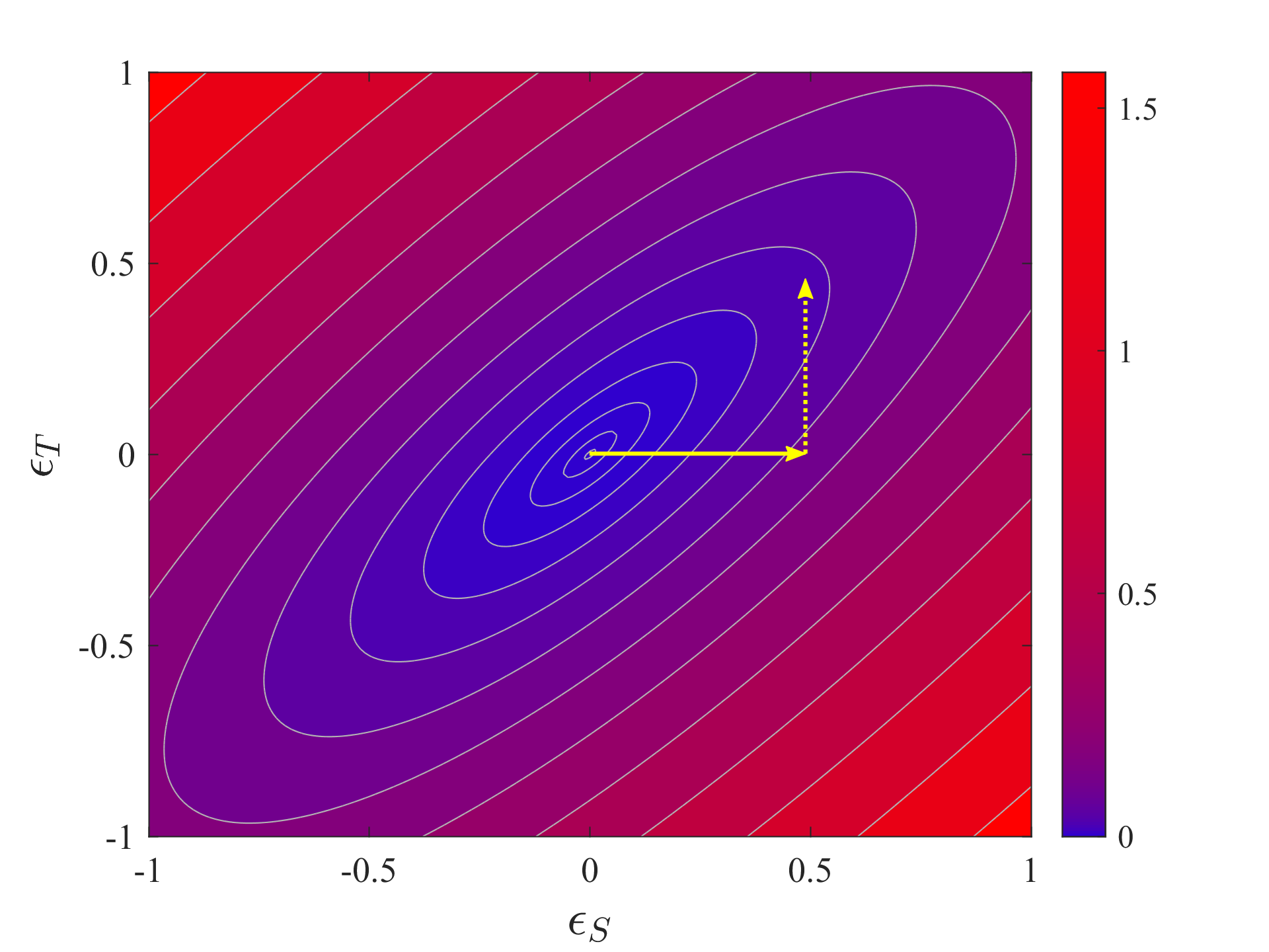
Figure 1: An illustration of the energy as function of the source strain and target strain. The locations of the nodes are defined by force balance. The response is obtained by applying a source strain (full arrow) $\epsilon_{S}$, and then minimizing the energy to find $\epsilon_{T}$ (dotted arrows).

Training global response

We begin by training an auxetic response, defined in terms of the Poisson’s ratio $\nu$. To measure it, we apply a uniaxial strain, $\epsilon_{S}$, along the $x$ direction and measure the resulting transverse strain along the $y$ direction, $\epsilon_{T}$. The Poisson’s ratio is defined as $\nu=-\frac{\epsilon_{T}}{\epsilon_{S}}$; auxetic materials have $\nu<0$. Within linear response, for an isotropic $d$-dimensional solid, $\nu<0$ corresponds to a ratio of the shear modulus $G$ to bulk modulus $B$ that satisfies $G/B>d/2$. We will also consider the non-linear regime where the Poisson’s ratio may depend on the magnitude of the imposed strain $\epsilon_{S}$.

To train our networks, we apply periodic strain cycles of isotropic compression and expansion in the continuous range $\left[-\epsilon_{Age},\epsilon_{Age}\right]$. The goal of this is to reduce the energy along the direction $\epsilon_{T}=\epsilon_{S}$. We let the system age during the entire cycle so that a smooth continuous valley is created.

Because the aging rate increases with the stress in the system, the functional form of the training strain $\epsilon_{tr}$ as a function of time, $\epsilon_{tr}\left(t\right)$, affects the outcome. Aging is most rapid at strains $\left|\epsilon_{tr}\right|\approx\epsilon_{Age}$ and much slower when $\left|\epsilon_{tr}\right|\approx 0$. To compensate for this effect, we choose a functional form that emphasizes small strains, $\epsilon_{tr}\left(t\right)=-\epsilon_{Age}\left[g\left(t\right)\right]^{3}$, where $g\left(t\right)$ is a periodic triangle waveform with unit amplitude . Note that after an integer number of cycles, the energy minimum often differs from zero strain. It is convenient for $\epsilon=0$ to be the energy minimum, and therefore at the end of the training phase we also age the system at zero strain before measuring the elastic properties.

In Fig. 2(a), we show the evolution of the Poisson’s ratio as a function of the strain at which it is measured $\epsilon$, as the network is aged for an increasing number of compression/expansion cycles. Initially the Poisson’s ratio is $\nu\approx 0.4$ and is only very weakly dependent on strain. As the number of cycles grows, the Poisson’s ratio decreases, especially near zero strain. The Poisson’s ratio is minimal at $\epsilon=0$ and increases with $\epsilon$ for both positive and negative strains. For a large number of cycles, $\nu\left(\epsilon\rightarrow 0\right)$ approaches $-1$, which is the lowest possible value allowed for an isotropic solid.

By aging at different strain amplitudes $\epsilon_{Age}$ we can control the range over which the Poisson’s ratio is minimal. Fig. 2(b) shows that $\nu\approx-1$ over the range $-\epsilon_{Age}\lesssim\epsilon\lesssim\epsilon_{Age}$. Thus, the response of the system contains a memory of the range of strains over which the system was aged. Moreover, the response is approximately linear ($\nu$ is nearly independent of $\epsilon$) in this range. This allows the maximum training strain $\epsilon_{Age}$ to be read out as the strain at which Poisson’s ratio starts to depend strongly on strain. These results show that plastic deformation in the $\ell$-model encodes memory stored in the material of the applied strains, as has also been proposed for selecting folding pathways in origami stern2019learned .

The evolution of the energy required to expand the system to a strain $\epsilon$ as a function of strain is shown in Fig. 2(c). To emphasize the relative change at different strains we normalize the energy, $U\left(\tau,\epsilon\right)$ of the system at strain $\epsilon$ applied after $\tau$ aging cycles, by the energy before the system was aged, which is approximately quadratic in $\epsilon$. In the range $-\epsilon_{Age}\lesssim\epsilon\lesssim\epsilon_{Age}$ the energy is greatly lowered, decreasing by several orders of magnitude, while at larger strains the change is more moderate.

Figure 2: Aging under periodic cycles of isotropic compression and expansion. (a) The Poisson’s ratio $\nu$ versus measurement strain $\epsilon$ for different numbers of cycles, $\tau$. (b) The Poisson’s ratio for different maximum aging strains, $\epsilon_{Age}$, after $\tau=5\cdot 10^{4}$ cycles. The Poisson’s ratio is near $-1$, in the range $-\epsilon_{Age}\lesssim\epsilon\lesssim\epsilon_{Age}$. Dashed lines denote $\pm\epsilon_{Age}$. (c) The energy required for isotropic expansion and compression, $U_{Age}(\tau,\epsilon)$ versus isotropic strain $\epsilon$ after $\tau$ cycles, normalized by the energy of the unaged network. Note the energy is most suppressed at the limits of the training strain, $\epsilon_{Age}=0.025$. (d) The linear Poisson’s ratio at $\tau=500$ versus the ratio of the aging rate, $\Gamma$, to the cycle frequency, $\omega$.

We now discuss the optimal amplitude and frequency for periodic driving in order to direct aging. First, we note that Fig. 2(b) shows that the desired Poisson’s ratio $\nu=-1$ is approached at sufficiently high values of the amplitude of the training strain, $\epsilon_{Age}$. This is seen in Fig. 2(d), which shows the Poisson’s ratio at a constant aging time. Increasing $\epsilon_{Age}$ results in a lower value of $\nu$. Aging at high strains causes bigger changes in the structure, which, in turn, have a bigger effect on the elastic properties. Large strains are even more important in materials where plasticity occurs only above a threshold strain.

The next consideration is the frequency of the training strain. There are two competing scales: (i) the frequency of the driving, $\omega$, and (ii) the aging rate $\Gamma=\gamma k$ defined below Eq. 1. Recall that aging is faster when the strains are larger. The effective aging rate $\Gamma_{eff}$ therefore depends not only on $\Gamma$ but on the aging strain: $\Gamma_{eff}=\Gamma\epsilon_{Age}$.

If aging occurs at a rate which is high with respect to the frequency of the driving cycle, then the energy will be minimized at each strain during the cycle. On the other hand if the aging rate is slow then the system will not evolve much. We therefore, expect that aging is optimal at an intermediate value, when $\Gamma_{eff}\sim\omega$. In Fig. 2(d) we show the Poisson ratio within linear response versus $\Gamma/\omega\equiv\Gamma_{eff}/\left(\omega\epsilon_{Age}\right)$ at a fixed aging time. In these calculations, $\omega$ is held constant. The effectiveness of aging can be measured by the amount the Poisson’s ratio has decreased. The minimum of $\nu$, therefore, is an indication of the optimal aging rate. The position of the minimum in $\nu$ shifts to lower values of $\Gamma_{eff}/\left(\omega\epsilon_{Age}\right)$ with increasing $\epsilon_{Age}$, a trend that is consistent with expectation.

Aging under periodic isotropic strain is far more effective in producing an auxetic response than aging at a comparable fixed isotropic strain. Fig. 2(b) shows that for a large enough number of cycles, we reach $\nu\approx-1$ over the range of measuring strains of $-\epsilon_{Age}\lesssim\epsilon\lesssim\epsilon_{Age}$ even for small $\epsilon_{Age}$. Aging at a fixed strain of $\epsilon_{Age}$, however, only decreases the Poisson’s ratio under compression hexner2019nonlinear , and by a far smaller amount. At a fixed aging isotropic expansion, $\nu$ actually becomes more positive. For fixed aging strains, it requires large compressions to become auxetic, and even then $\nu$ is significantly less negative than for periodic driving. Although the change in response is small over one cycle of driving at small $\epsilon_{Age}$, the changes accumulate over many cycles, eventually leading to dramatic effects.

We also consider another form for the strain as a function of time: cyclically switching between $\epsilon=-\epsilon_{Age}$ and $\epsilon_{Age}$ with a square-wave form, shown in Fig. 3(a). This lowers the energy predominantly at the strains $\epsilon_{Age}$ and $-\epsilon_{Age}$. As a result this allows the system to develop two distinct energy minima, thus allowing bi-stability. This is demonstrated in Fig. 3(b). The energy barrier grows with the amplitude of the training strain.

Constructing materials with multiple minima allows the creation of materials with discrete states with potentially different elastic properties. Elastic networks with bistable springs have been shown to self-organize in various ways in response the periodic forcing Kedia2019 and have been useful to encode multiple memories stern2019learned .

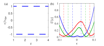
Figure 3: Training a bistable energy landscape. (a) The strain as a function of time applied as the system ages. (b) The energy for expansion as a function of measuring strain after $T=10^{4}$ cycles of training. The dashed lines denote $\epsilon_{Age}$ and $-\epsilon_{Age}$.

Training allosteric response

We next consider spatially heterogeneous responses, focusing on the biologically-inspired response of allostery rocks2017designing ; yan2017architecture where the strain on a pair of source nodes results in a strain on a pair of target nodes. For convenience, each pair of source and target nodes corresponds to the nodes of a randomly chosen bond (that is subsequently removed). The source and target are chosen to be at least half the system length apart (an example is shown in Fig. 4(d)).

In the initial unstressed networks the distance between the source nodes is denoted by $\ell_{S,0}$, and under an imposed strain by $\ell_{S}$; the source strain is defined to be $\epsilon_{S}=\ell_{S}/\ell_{S,0}-1$. In general, the aim is to produce a target strain $\epsilon_{T}=\ell_{T}/\ell_{T,0}-1$ between the target nodes that is given by $\epsilon_{T}=\Delta\epsilon_{S}$. For simplicity, we will consider the cases $\Delta=\pm 1$, where squeezing the source nodes results in a strain between target nodes of the same magnitude, but with a sign that can be chosen to be either positive or negative.

We begin by training nearly isostatic networks. we strain both the source and target nodes periodically, at a training strain amplitude of $\epsilon_{Age}$, as the system evolves. To produce a target response with $\Delta=1$ the source and training strains are in phase with each other; to produce a target response with $\Delta=-1$, the source and training strains are $\pi$ out of phase. After each cycle of training, we turn off aging to apply one cycle of strain to the source only, and measure the corresponding strain at the target. We then turn the aging back on, train for another cycle and again turn the aging off for another measurement cycle. The results of each measurement cycle are shown in Fig. 4(a). We show the cycles of source strain $\epsilon_{S}/\epsilon_{Age}$ in green and the measured target strain $\epsilon_{T}/\epsilon_{Age}$ in red as a function of the number of training cycles $\tau$ that the system has undergone, for a training designed to produce $\Delta=1$. Initially, the response at the target is very weak but it grows increasingly stronger as the training continues. At long times, the response approaches the desired amplitude: $\epsilon_{T}=\epsilon_{S}$.

To characterize the effectiveness of training, we measure $\epsilon^{max}_{T}$, the absolute value of $\epsilon_{T}$ at the largest amplitude of the source strain, $\epsilon^{max}_{S}=\epsilon_{Age}$. For a completely successful training, $\epsilon^{max}_{T}/\epsilon^{max}_{S}=\mid{\Delta}\mid$=1. In Fig.  4(b) we show $\epsilon^{max}_{T}/\epsilon^{max}_{S}$ versus the number of training cycles. At long times, the average changes slowly and appears to settle at a value that depends only weakly on $\epsilon^{max}_{S}$. At aging strains $\epsilon_{Age}\leq 0.5$, on average $\epsilon^{max}_{T}$ reaches above $90\%$ of its target amplitude, $\epsilon^{max}_{T}=\epsilon_{Age}$. Training is therefore highly successful even far in the nonlinear regime, producing a target strain that is nearly equal to the source strain even at $\epsilon^{max}_{S}=0.5$ where the distance between the two source nodes is 50% higher than the distance in the absence of strain.

Note that the results shown in Fig. 4(b) correspond to an average over an ensemble of $50$ networks. Fig. 4(c) shows the distribution of the asymptotic values of $\epsilon^{max}_{T}/\epsilon^{max}_{S}$ for the different networks in the ensemble after many cycles of training $\tau$. While most of the networks achieve precisely the targeted response, a fraction of the realizations fail completely to do so. In the inset of Fig. 4(c) we show that the fraction of failed realizations grows with $\epsilon_{Age}$. Our results suggest that a class of low-coordination nodes may play an important role in the cases of failure. Networks derived from jammed packings near the isostatic point, $\Delta Z\approx 0$, are known to have some nodes with only three bonds in two dimensions. Often two of those bonds meet at angles near $180^{\circ}$ and are thus unable to support large forces hexner2018linking without buckling; such nodes are known as bucklers. Squeezing those bonds results in a localized response Charbonneau2015 . We find that if the source and target nodes are allowed to include bucklers, approximately 30% of networks cannot be tuned at large strain. The analysis showed in Fig. 4(c) excludes bucklers at the source and target. Even so, approximately 10% of the networks are untunable, perhaps because bucklers near the source and target nodes inhibit strong responses at high deformations.

In the nearly isostatic networks discussed so far, we achieve a high degree of success in training allostery by applying strains only to the source and target nodes while the remaining bonds evolve through plastic deformations. The decay of stresses away from a squeezed bond is governed by an important length scale, $\xi$ that diverges as the coordination is decreased towards isostaticity ellenbroek2006critical . At distances $r<<\xi$ the decay is very slow, and is almost independent of distance while at $r>>\xi$ there is a crossover to a rapid decay, $r^{-d}$, as expected from continuum elasticity ellenbroek2006critical ; lerner2014breakdown . When $\xi$ is larger than the distance between the source and target, the strategy of applying a periodic training strain to the source and target bonds is useful. This is why we achieve a high degree of success in tuning nearly isostatic networks.

However, in more highly coordinated networks, where $\xi$ is small in comparison to the distance between the source and target node pairs, the region in between those two pairs is nearly unaffected by the aging since the strains are negligible. In that case, only bonds near the source and target age significantly, and the source and target never become coupled by the applied strains.

To overcome this limitation, we introduce applied strains on additional pairs of nodes, which we call “repeaters”. The goal of the repeaters is to couple the source and target by rebroadcasting the elastic signal. Each repeater is a randomly chosen pair of nearby nodes, as illustrated in Fig. 4(d). During the training cycle the repeater nodes are strained periodically with an amplitude $\epsilon_{Age}$, and with a phase, $0$ or $\pi$, chosen randomly. As with the source and target, the bond between the nodes of each repeater is removed prior to aging. Thus, training does not distinguish between the source, target and repeater nodes. However, during readout, only the source is strained, by $\epsilon_{S}$, while the resulting strain at the target, $\epsilon_{T}$, is measured.

Figure 4(e) shows $\epsilon^{max}_{T}/\epsilon^{max}_{S}$ after the system has reached its asymptotic value for a large number of training cycles, as a function of the fraction of repeater node pairs. For $\Delta Z\approx 0.52$ the response is maximal when $4\%$ of the node pairs are repeaters. This corresponds to the length scale between repeaters of $\sim 5\langle ell_{0}\rangle$, consistent with the length scale measured in Ref. lerner2014breakdown . To ensure that the increase of $\epsilon^{max}_{T}/\epsilon^{max}_{S}$ is not the result of bond removal between pairs of repeater nodes, we also show in Fig. 4(e) the effect of training when an equivalent number of bonds are removed at random. This has a much smaller effect.

While our goal is to train the response of a specific target when the source is strained, the training protocol does not distinguish between the source, target and the repeaters. This implies that straining the source nodes also results in an allosteric response in each of the repeaters. Thus, this system achieves multifunctional behavior, where a single source controls the response at many sites, similar to that studied in Ref. rocks2019limits . Our results show that it is easier to train multifunctional response in a system in which the targets are spaced approximately a distance $\xi$ apart than it is to train a system with a single target that is at a distance from the source that is large compared to $\xi$.

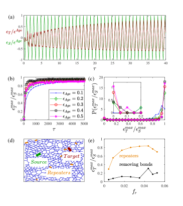
Figure 4: (a) The evolution, at short times, of the allosteric response as a function of the number of training cycles $\tau$. After each training cycle we measure the strain on the target nodes (red), $\epsilon_{T}$ in response to a strain on the source nodes (green), $\epsilon_{S}$. The maximum value of $\epsilon_{S}$, $\epsilon^{max}_{S}$, during the measurement cycle is taken to be the maximum training strain $\epsilon_{Age}$. At large times the maximum value of the target strain, $\epsilon^{max}_{T}$, converges to its target value: $\epsilon^{max}_{T}=\epsilon_{Age}$. (b) $\epsilon^{max}_{T}/\epsilon^{max}_{S}$ as a function of the number of training cycles $\tau$. Training at near isostatic connectivity is highly successful even far from the linear regime. (c) The distribution of $\epsilon^{max}_{T}/\epsilon^{max}_{S}$ at the largest times measured in (b), using the same color/symbol scheme. Note that the distribution is bimodal: at large $\epsilon_{Age}$ most of the realizations achieve their targets but a small fraction fail nearly completely, with $\epsilon^{max}_{T}/\epsilon^{max}_{S}\approx 0$. Inset: a zoomed view of the distribution at small $\epsilon^{max}_{T}/\epsilon^{max}_{S}$ shows that more networks fail as $\epsilon_{Age}$ increases. (d) An illustration of a network that we train. At large connectivity, we also strain randomly chosen “repeater” bonds during training. (e) Training at high connectivity using “repeaters." For $\Delta Z\approx 0.52$ the optimal number of repeaters is near 4%.

Discussion

In this paper we demonstrated that a model that undergoes creep can be trained to develop unusual mechanical responses well into the non-linear regime. These can be either global, such as auxetic responses, or spatially heterogeneous, as in a long-ranged allosteric response. Allostery can be considered as a “Green’s function” that characterizes how a local input strain is transmitted to a far distant local site. Thus, if allostery can be trained into the system then presumably almost any response can be achieved.

The central strategy that we have introduced is based on creating a low-energy valley that couples the source and target strains. This is a curve defined by the target strain as a function of the source strain $\epsilon_{T}\left(\epsilon_{S}\right)$. In this paper we focused on the simplest case, $\epsilon_{T}\propto\epsilon_{S}$; more generally this curve can be non-linear, and non-monotonic leading to more complex responses. Straining periodically along this curve lowers the energy along the entire path. This is a collective effect: driving a small number of degrees of freedom results in changes to the entire system.

This directed aging approach exploits the natural optimization occurring in an aging system. It does not require an initial carefully designed structure nor a careful manipulation at the microscopic scale during the aging process. As a result this method of creating novel function in materials is easily scaled up to systems of arbitrarily large size.

Our dynamics can be considered a learning rule by which a system learns a specific motion. The results presented here fit into a broad set of problems in which systems learn by example, such as neural networks. In this class of problems, a large number of variables are optimized to satisfy a complex constraint. In our system optimization occurs naturally as the system lowers its energy. This suggests that this is a platform for mechanical machine learning.

We thank Nidhi Pashine, Chukwunonso Arinze, Paul Chaikin and Arvind Murugan for useful discussions. Work was supported by the NSF MRSEC Program DMR-1420709 (NP), NSF DMR-1404841(SRN) and DOE DE-FG02-03ER46088 (DH) and the Simons Foundation for the collaboration “Cracking the Glass Problem” awards $\#$348125 to SRN and $\#454945$ to AJL, and Investigator award $\#$327939 to AJL. We acknowledge support from the University of Chicago Research Computing Center.

References

- (1) M. S. Kushwaha, P. Halevi, L. Dobrzynski, and B. Djafari-Rouhani. Acoustic band structure of periodic elastic composites. Phys. Rev. Lett., 71:2022–2025, Sep 1993.
- (2) Tom Mullin, S Deschanel, Katia Bertoldi, and Mary C Boyce. Pattern transformation triggered by deformation. Physical review letters, 99(8):084301, 2007.
- (3) Katia Bertoldi, Vincenzo Vitelli, Johan Christensen, and Martin van Hecke. Flexible mechanical metamaterials. Nature Reviews Materials, 2(11):17066, 2017.
- (4) Zachary G Nicolaou and Adilson E Motter. Mechanical metamaterials with negative compressibility transitions. Nature materials, 11(7):608, 2012.
- (5) CL Kane and TC Lubensky. Topological boundary modes in isostatic lattices. Nature Physics, 10(1):39, 2014.
- (6) Bryan Gin-ge Chen, Nitin Upadhyaya, and Vincenzo Vitelli. Nonlinear conduction via solitons in a topological mechanical insulator. Proceedings of the National Academy of Sciences, 111(36):13004–13009, 2014.
- (7) Jia Liu, Tianyu Gu, Sicong Shan, Sung H Kang, James C Weaver, and Katia Bertoldi. Harnessing buckling to design architected materials that exhibit effective negative swelling. Advanced Materials, 28(31):6619–6624, 2016.
- (8) Corentin Coulais, Eial Teomy, Koen de Reus, Yair Shokef, and Martin van Hecke. Combinatorial design of textured mechanical metamaterials. Nature, 535(7613):529, 2016.
- (9) Jason W Rocks, Nidhi Pashine, Irmgard Bischofberger, Carl P Goodrich, Andrea J Liu, and Sidney R Nagel. Designing allostery-inspired response in mechanical networks. Proceedings of the National Academy of Sciences, 114(10):2520–2525, 2017.
- (10) Le Yan, Riccardo Ravasio, Carolina Brito, and Matthieu Wyart. Architecture and coevolution of allosteric materials. Proceedings of the National Academy of Sciences, 114(10):2526–2531, 2017.
- (11) Michael R Mitchell, Tsvi Tlusty, and Stanislas Leibler. Strain analysis of protein structures and low dimensionality of mechanical allosteric couplings. Proceedings of the National Academy of Sciences, 113(40):E5847–E5855, 2016.
- (12) Nidhi Pashine, Daniel Hexner, Andrea J Liu, and Sidney R Nagel. Directed aging, memory and nature’s greed. arXiv preprint arXiv:1903.05776, 2019.
- (13) Roderic Lakes. Foam structures with a negative poisson’s ratio. Science, 235(4792):1038–1040, 1987.
- (14) D. J. Durian. Foam mechanics at the bubble scale. Phys. Rev. Lett., 75:4780–4783, 1995.
- (15) Corey S. O’Hern, Leonardo E. Silbert, Andrea J. Liu, and Sidney R. Nagel. Jamming at zero temperature and zero applied stress: The epitome of disorder. Phys. Rev. E, 68:011306, 2003.
- (16) Andrea J Liu and Sidney R Nagel. The jamming transition and the marginally jammed solid. Annu. Rev. Condens. Matter Phys., 1(1):347–369, 2010.
- (17) Daniel Hexner, Nidhi Pashine, Andrea J Liu, and Sidney R Nagel. Effect of aging on the non-linear elasticity and memory formation in materials. arXiv preprint arXiv:1909.00481, 2019.
- (18) James Clerk Maxwell. Iv. on the dynamical theory of gases. Philosophical transactions of the Royal Society of London, (157):49–88, 1867.
- (19) Michael F Staddon, Kate E Cavanaugh, Edwin M Munro, Margaret L Gardel, and Shiladitya Banerjee. Mechanosensitive junction remodelling promotes robust epithelial morphogenesis. bioRxiv, page 648980, 2019.
- (20) Kate E Cavanaugh, Michael F Staddon, Ed Munro, Shiladitya Banerjee, and Margaret L Gardel. Rhoa mediates epithelial cell shape changes via mechanosensitive endocytosis. bioRxiv, page 605485, 2019.
- (21) Larger exponents age strains more uniformly, however they require a finer discretization.
- (22) Menachem Stern, Matthew B Pinson, and Arvind Murugan. Learned multi-stability in mechanical networks. arXiv preprint arXiv:1902.08317, 2019.
- (23) Hridesh Kedia, Deng Pan, Jean-Jacques Slotine, and Jeremy L. England. Drive-specific adaptation in disordered mechanical networks of bistable springs. arXiv preprint arXiv:1908.09332, 2019.
- (24) Daniel Hexner, Andrea J Liu, and Sidney R Nagel. Linking microscopic and macroscopic response in disordered solids. Physical Review E, 97(6):063001, 2018.
- (25) Patrick Charbonneau, Eric I. Corwin, Giorgio Parisi, and Francesco Zamponi. Jamming criticality revealed by removing localized buckling excitations. Phys. Rev. Lett., 114:125504, 2015.
- (26) Wouter G Ellenbroek, Ellák Somfai, Martin van Hecke, and Wim van Saarloos. Critical scaling in linear response of frictionless granular packings near jamming. Physical review letters, 97(25):258001, 2006.
- (27) Edan Lerner, Eric DeGiuli, Gustavo Düring, and Matthieu Wyart. Breakdown of continuum elasticity in amorphous solids. Soft Matter, 10(28):5085–5092, 2014.
- (28) Jason W Rocks, Henrik Ronellenfitsch, Andrea J Liu, Sidney R Nagel, and Eleni Katifori. Limits of multifunctionality in tunable networks. Proceedings of the National Academy of Sciences, 116(7):2506–2511, 2019.