Algebraic entropy computations for lattice equations: why initial value problems do matter

Abstract

In this letter we show that the results of degree growth (algebraic entropy) calculations for lattice equations strongly depend on the initial value problem that one chooses. We consider two problematic types of initial value configurations, one with problems in the past light-cone, the other one causing interference in the future light-cone, and apply them to Hirota’s discrete KdV equation and to the discrete Liouville equation. Both of these initial value problems lead to exponential degree growth for Hirota’s dKdV, the quintessential integrable lattice equation. For the discrete Liouville equation, though it is linearizable, one of the initial value problems yields exponential degree growth whereas the other is shown to yield non-polynomial (though still sub-exponential) growth. These results are in contrast to the common belief that discrete integrable equations must have polynomial growth and that linearizable equations necessarily have linear degree growth, regardless of the initial value problem one imposes. Finally, as a possible remedy for one of the observed anomalies, we also propose basing integrability tests that use growth criteria on the degree growth of a single initial value instead of all the initial values.

1 Introduction

By now it is common knowledge that discrete integrable systems possess some beautiful underlying mathematical structures. For example, in the case of integrable bi-rational mappings, insights from algebraic geometry have led to the development of rigorous criteria (and tests) for integrability [1, 2, 3, 4], and to a widely accepted definition of an integrable mapping: it must have zero algebraic entropy [5]. The algebraic entropy for a rational mapping is defined as

$$E=\lim_{n\to\infty}\frac{\log(d_{n})}{n},$$

where $d_{n}$ is the degree of the $n$th iterate of the mapping, and can be thought of as measuring the complexity of the mapping, in the sense of Arnold [6]. Note that $E\geq 0$ and that it is non-zero only if the degree growth is exponential.

The situation for lattice equations, however, is very different and a definition of integrability in that context remains elusive. (As a general reference see [7].) Attempts have been made to introduce to the lattice setting certain integrability criteria that proved useful in the context of mappings, such as algebraic entropy [8, 9, 10], but in this letter we wish to warn against any such attempt that does not take into account the crucial role that initial value problems play in the lattice setting.

1.1 The lattice setting

In this letter we only consider lattice equations, i.e. partial difference equations, defined on the basic elementary square or quadrilateral of the $\mathbb{Z}^{2}$ lattice, see Figure 1. Such equations are called quad equations. The four corner values of the $2\times 2$ stencil are related by a multi-linear equation

$$Q(x_{n-1,m-1},x_{n,m-1},x_{n,m-1},x_{n,m})=0,$$ (1)

which may also contain various parameters.

Figure 1: The elementary square in the $\mathbb{Z}^{2}$ lattice. The independent variable $n$ grows to the right, $m$ grows upward.

Any multi-linear quad equation allows propagation or evolution once suitable initial data is given, for example on a staircase or on a corner, as in Figure 2, but here we shall also consider some more exotic initial value problems. Note however that all initial value problems we shall consider are well-posed in the sense of [11].

Figure 2: a) The Cartesian lattice with given corner-type initial values (at black discs) from which one can then compute the values at open discs in the upper right quadrant. b) The same with a staircase of initial values.

In this letter we illustrate our results using two quad equations:

• Liouville equation:

  $$x_{n,m}x_{n-1,m-1}-x_{n,m-1}x_{n-1,m}=1,$$ (2)

  which linearizes to (non-autonomous) second order ordinary difference equations, in the $n$ as well as in the $m$ direction.

• Hirota’s discrete KdV equation

  $$x_{n,m}-x_{n-1,m-1}=\frac{1}{x_{n,m-1}}-\frac{\lambda}{x_{n-1,m}},$$ (3)

  which is integrable for $\lambda=1$ but non-integrable for any other non-zero value of $\lambda$.

1.2 Algebraic entropy

As already mentioned, one property that is believed to be strongly associated with integrability is zero Algebraic Entropy. For lattice equations (2) or (3), given initial values such as in Figure 2, $x_{n,m}$ at any of the open discs will be a rational function of the initial values given at the black discs in the past light-cone of that open disc, c.f. Figure 3. The degrees of the numerator and denominator of $x_{n,m}$ will grow as $n$ and $m$ grow, but if the system is integrable there will be cancellations and the growth slows down [1, 2, 13, 8].

Figure 3: Past and future light-cones, for equations (2) and (3), for the point $\otimes$ in the middle. The past light-cone contains all points that can influence the value at $\otimes$, while the future light-cone contains all points that can be influenced by the value at $\otimes$.

In [8] it was shown that for initial values as in Figure 2, Hirota’s discrete KdV equation (3) exhibits quadratic degree growth whereas the discrete Liouville equation (2) has linear degree growth (see also section 2.1). In fact, besides exponential growth (i.e. non-zero algebraic entropy), the degree growths that have been reported in the literature for lattice equations [9, 10] coincide with those observed for second order bi-rational mappings: bounded growth, linear growth or quadratic degree growth. Hence the ‘rule of thumb’ that is in common use today (cf. [2, 5, 12, 8, 14, 15])

• if the degree growth is linear in $n,m$ the equation is linearizable.

• if the degree growth is polynomial the equation is integrable.

• if the degree growth is exponential the equation is not integrable.

It is important to stress that although the above statements can be considered to be rigorous in the context of second order bi-rational mappings [16], when it comes to lattice equations these should be thought of as mere experimental observations.

In this letter we will discuss how the form of the initial value boundary may influence degree growth computations and distort the algebraic entropy results. We concentrate on two particular effects that have their origin in:

1. The number of initial values in the past light-cone. Usually this number grows linearly, but it may in fact grow faster.

2. The number of initial values in the future light-cone. Usually there are none but for some allowed (well-posed) initial value problems this number can be non-zero.

In this letter we will only discuss what can happen for the Liouville equation (2) and for Hirota’s discrete KdV (3) equation, both defined on a $2\times 2$ stencil, and we shall report work on other kinds of stencils elsewhere.

2 Growth results for various initial value problems

2.1 Corner initial values

Let us first consider conventional corner initial values as in Figure 2a. Figure 4 shows the degrees of the numerator in $x_{n,m}$ for the Liouville equation (2), which are given by $d_{n,m}=n+m$, and for Hirota’s KdV equation (3) with $\lambda=1$: $d_{n,m}=4nm-2\max(n,m)+1$ (cf. [8]). As before, black discs depict initial values.

Figure 4: a) For the Liouville equation (2) the degree growth is linear, as expected: $d_{n,m}=n+m$. b) Hirota’s KdV equation (3) for $\lambda=1$ is integrable and the degree rule is $d_{n,m}=4nm-2\max(n,m)+1$ (see also [8]).

Figure 5 gives the degrees for a non-integrable version ($\lambda=2$) of Hirota’s KdV equation and this time the growth is exponential. The first difference between the integrable and non-integrable versions occurs at lattice points $(2,3)$ and $(3,2)$ where the integrable version has a numerator of degree 19 while the non-integrable one has degree 22. One can easily compute the corresponding rational functions $x_{n,m}$. It turns out that for any $\lambda$ the denominator of $x_{3,2}$ has the degree 3 factor

$$x_{1,0}\ x_{0,1}\ x_{0,0}-x_{1,0}\ \lambda+x_{0,1}.$$

If we now insist that this should also be a factor of the numerator (in order to have cancellations) one finds that this is only possible if $\lambda=1$ or $0$.

Figure 5: Hirota’s KdV with $\lambda=2$ (non-integrable). On the diagonal the growth is exponential, approximately $0.85\cdot 3.7^{n}$. It can be shown however (see section 2.3) that the asymptotic degree growth on the diagonal is actually $\propto 4^{n}$.

2.2 Problems originating in the past light-cone

For a quad equation and with evolution to the NE direction, the initial values $f_{\alpha,\beta}$ that appear in $x_{n,m}$ are those in its past light-cone, except that of the $f_{\alpha,m}$ the only initial value that is included is the first to the left. Possible problems with the past light cone are illustrated in Figures 6 and 7. Let us first take a closer look at the computations in the case of the Liouville equation. In Figure 6 we use numbering in which the rightmost column is at $n=0$. For the first two points in that column we find

$$x_{0,1} = \frac{f_{0,0}\ f_{-1,1}+\lambda}{f_{-1,0}},$$ (4)

$$x_{0,2} = \frac{f_{0,0}\ {f_{-1,1}}^{2}\ f_{-2,1}\ f_{-3,1}\ f_{-4,2}+l.o.}{f_{-1,1}\ f_{-1,0}\ f_{-2,1}\ f_{-3,1}\ f_{-4,1}}.$$ (5)

Thus $x_{0,2}$ depends on all initial values of type $f_{n,0}$ and $f_{n,1}$ but only on $f_{-4,2}$ in the $m=2$ row, i.e. it depends on 7 initial values and the highest degree term depends on exactly 6 of them.

Figure 6: Liouville equation for a left-leaning parabolic boundary. Bullets depict the initial values. The degrees in the rightmost column grow as $m(m+1)$.

Figure 7: Hirota’s KdV with parabolic boundary to the left. The growth in the rightmost column is now cubic, $\frac{1}{6}(8m^{3}-9m^{2}+25m-9)\pm\frac{1}{2}$.

Usually the number of initial values in the past light-cone grows linearly with $n$ or $m$; this is what happens for the corner and staircase initial configurations of Figure 2. However, if the number of initial values grows quadratically with $m$ (as in the case of the boundaries in Figures 6 and 7 where it grows as $m^{2}+m+1$) then complexity grows one unit faster: the degree growth in the $m$ direction is quadratic for Liouville and cubic for Hirota’s KdV, as can be seen from Figure 7. But the complexity can be made to grow exponentially for Hirota’s KdV or even for Liouville, if the initial values for the left-hand boundary are located for example at $-2^{m}\leq n\leq-2^{m-1}$.

The effects induced by a faster-than-linear growth of the number of initial values in the past light-cone, illustrated above, are fairly interesting by themselves. However, if we wish to use degree growth as an objective criterion and, most importantly, as a tool for identifying integrable lattice equations then these effects are best eliminated.

One solution would be to consider the degree growth with respect to only a single initial value. (In practical computations all other initial values can then be numerical.) Such an approach is illustrated in Figures 8 and 9.

Figure 8: Degrees w.r.t an individual initial value: Liouville equation. With the linear growth of the boundary eliminated the degree growth is bounded.

In each of these figures the missing corner point is taken to be at $(0,0)$ and the sole initial value at $(1,1)$. The initial values $f_{1,m}\,(m>1)$ and $f_{n,1}\,(n>1)$ are numerical. For the Liouville equation the degrees are then bounded ($d_{n,m}=\min(n,m,2)$) whereas for the usual, integrable, version of Hirota’s KdV the degrees in Figure 9a) are given by $d_{n,m}=2\min(n,m)-1$, i.e. they now exhibit linear growth.

Figure 9: Degrees w.r.t an individual initial value: Hirota’s KdV for $\lambda=1$ (integrable) and $\lambda=2$ (non-integrable). When the linear growth of the boundary is eliminated the degrees in the integrable case grow linearly, while for the non-integrable cases the degrees still grow exponentially.

For the non-integrable version of Hirota’s KdV equation of Figure 9b) the growth is still exponential. It is interesting to observe that the degrees in Figures 9b) and 5 satisfy very similar recursion relations:

$$d_{n,m}=d_{n-1,m}+d_{n,m-1}~{}~{}(n\neq m)\quad{\rm and}\quad d_{n,n}=d_{n-1,n}+d_{n,n-1}+1,$$

for Figure 9b) and

$$d_{n,m}=d_{n-1,m}+d_{n,m-1}+2~{}~{}(n\neq m)\quad{\rm and}\quad d_{n,n}=d_{n-1,n}+d_{n,n-1}+3,$$

for Figure 5. In fact, the number sequence on the diagonal in Figure 9b) is known, it is sequence M2811 or A006134 in [17] and it can be shown to grow asymptotically as $4^{n}$. As the only difference between the settings in Figure 9b) and Figure 5 is that in the latter the number of initial values grows linearly with $n$ and $m$, whereas in Figure 9b) there is only a single initial value, it follows that asymptotically the degrees on the diagonal in Figure 5 should grow at least as fast as $4^{n}$. It can be shown that this is indeed the exact asymptotic growth rate.

In summary, if we only measure the degree growth with respect to a single specific initial value (as opposed to all initial values as one does in standard algebraic entropy calculations) any problems due to the past light-cone are eliminated. One may say that the effects from the past light-cone are “additive” and by choosing only one initial value as independent variable we can take care of this artefact. An added bonus of this approach is that, in practice, instead of symbols one can assign numerical values to all other initial values, which dramatically reduces the calculation time. Obviously, finding even just a single set of such values for which the degree growth becomes exponential is sufficient to show that the equation exhibits exponential degree growth in the usual sense. But if the aim is to establish integrability by showing that exponential growth is absent from the system, then of course one has to perform the calculations with greater care and verify that the result does not depend on the specifics of the numerical initial values or, indeed, on the choice of position for the initial value for which the degree is calculated.

2.3 Problems originating in the future light-cone

If the boundary on which the initial values are given intersects the future light-cone, the effect on the degree growth can be even more dramatic than in the previous case. With such a boundary there can be (from the viewpoint of integrability tests) potentially catastrophic interference when new independent variables—i.e. initial values—prevent cancellations. Such interference will result in much faster degree growth than one would find for ordinary corner or staircase-type initial value problems.

One such case is illustrated in Figure 10 for Hirota’s discrete KdV equation.

Figure 10: The integrable Hirota dKdV with 45 degree corner configuration. Along the horizontal axis the growth is linear after the first 2 lattice points, but along the diagonal the growth is exponential $d_{n,n}=3(2^{n}-1)$ and next to it $9(2^{n-1}-1)-2n$.

Instead of a vertical boundary as one would have in a corner-type initial value problem, we now have a $45^{o}$ forward leaning boundary. Note that the upper boundary is not a staircase and therefore evolution is well defined, i.e. the initial value problem is well-posed. (A staircase would allow evolution to the SE direction, conflicting eventually with evolution starting from the bottom boundary.) We observe that on the diagonal the degree growth is exponential, $d_{n,n}=3(2^{n}-1)$, and that one step to the right from the diagonal the degrees are given by $d_{n,n-1}=9(2^{n-1}-1)-2n$. After these first two steps the degree growth for a given $m$ as a function of $n$ is the same as in Figure 4 b), namely $(4m-2)n$. We note that for the Liouville equation the degrees in the $45^{o}$ corner region are in fact the same as in the $90^{o}$ corner of Figure 4a).

Above we have found that the past light-cone artefacts can be eliminated by calculating degrees with respect to just one independent variable among the initial values. It should be clear however that the same approach will not resolve problems that have to do with the future light-cone. For example, if we calculate the degree growth with respect to a single intial value for the initial value problem of Figure 10 we get the result in Figure 11.

Figure 11: The integrable Hirota dKdV with 45 degree corner configuration and a single variable . Along the diagonal the growth is exponential $d_{m,m}=2^{m-1}$ and for $n>m$ $d_{n,m}=3\ 2^{m-1}-2$.

Observe that the growth rate on the diagonal $m=n$ is $2^{m}$ for both cases. Though degree growth calculations with respect to a single initial value do not remove the problem, they do yield results that display it in a distilled form.

As mentioned before, when computing the degree growth with respect to a single initial variable all the other initial values can be taken as (generic) numerical values, and the degrees in Figure 11 are in fact obtained in this way. One could of course wonder why in such a calculation where all but a single initial value take numerical values, the growth on the diagonal in Figure 11 is so much faster than that on the diagonal for the corner initial value problem of Figure 9. But it should be noted that the values derived from the corner configuration are intricately related, allowing subtle cancellations, which is the reason for slow growth. If we replace these variables by random numbers the relations are eliminated and cancellations are no longer possible. (One can say that the future light-cone problems are “multiplicative” in nature.) Vice versa, we can note that the initial conditions on the vertical boundary in Figure 9 needed to reproduce these exact numerical values on the line $m=n+1$ are in fact increasingly complex rational expressions in the (sole) symbolic initial value.

Figure 12: Discrete Liouville equation in a step 3 wedge.

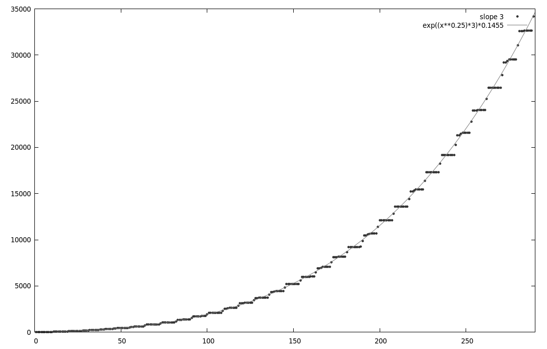
Figure 13: Same situation as in Figure 12 but for extended range. The vertical axis gives the degree of the numerator and the horizontal axis the order of iteration $n$. The approximate fit is with $d_{n,n}=0.1455\cdot\exp[3n^{\frac{1}{4}}]$.

We have also studied some other initial boundaries that can be problematic. One possibility is to have a wedge type boundary as in Figure 12 for the discrete Liouville equation. From the degrees on the shaded diagonal it is, at first, difficult to determine the rule for the degree growth but after computing more steps the type of growth on the diagonal becomes clearer, see Figure 13. There are regions of slow growth followed by jumps and we get a fairly good fit for the degree growth with the curve $0.1455\cdot\exp[3x^{\frac{1}{4}}]$, but similar fits with slightly different exponents are also possible. In all cases the exponent was found to be close to $x^{\frac{1}{4}}$ and thus asymptotically the growth is sub-exponential but faster than any polynomial: $an^{\alpha}<d_{n,n}<be^{\beta n}$ for all $\alpha,\beta>0$ (and suitable constants $a(\alpha),b(\beta)$), and the algebraic entropy as conventionally defined is still zero.

3 Summary

In this letter we have discussed how the choice of initial value problem can affect the degree growth in a lattice equation. Conventional initial value problems use corner or staircase boundaries, but one can have a well defined (well-posed) evolution starting with other kinds of initial value boundaries.

One of the problems we have identified concerns the number of initial values in a point’s past light-cone, which influences the subsequent degrees. In particular, for a boundary that recedes exponentially, we found that one can obtain exponential degree growth even for linearizable equations. In order to avoid any such ambiguous growth due to past light-cone effects, we propose to study the degree growth with respect to one individual initial value instead of all initial values. If this growth is polynomial, then its degree is one less than that for the conventional corner and staircase initial values. Moreover, in such a calculation the remaining initial values may be taken to be purely numerical, but in that case sufficient care must be taken to ensure that the choice of initial values does not influence the observed degree growth (e.g., due to accidental cancellations).

The situation is even more interesting and problematic in cases where the initial value boundaries intersect the future light-cone. We have shown that if, for Hirota’s discrete KdV equation, the boundary of the corner configuration is tilted forward to a $45^{o}$ angle, one can observe exponential degree growth even though the lattice equation is supposedly integrable. Another interesting finding is the behaviour in the wedge between sloping boundaries as in Figure 12. For the Liouville equation we find growth that is faster than polynomial but still sub-exponential. As far as the authors know this is the first time this type of degree growth has been observed in lattice equations.

As we have shown, when testing the degree growth for a lattice equation, it is imperative that one avoid initial value problems in which initial values appear in the future light-cones of the lattice points that one wishes to calculate. (It is not immediately clear however whether this simple safeguard is actually sufficient or whether there exist other boundary-induced effects that should be taken into account.)

In this letter we have presented results for two quad equations, the discrete Liouville equation and Hirota’s discrete KdV. However, we have obtained similar results also for Hirota’s bilinear KdV equation ($2\times 3$ stencil) and for the bilinear Toda lattice equation (star-shaped, 5 points.) For the Toda equation we have several rigorous results for the degrees which will be presented elsewhere.

While we have been discussing integrability from the point of view of the growth of complexity, there are other viewpoints as well, e.g. relying on symmetries and Lax pairs. One can then again ask whether a given initial value problem allows the construction of a sufficient number of symmetries or of a meaningful Lax pair [18, 19, 20, 21]. These approaches are for future consideration.

References

References

- [1] A.P. Veselov. Growth and integrability in the dynamics of mappings. Commun. Math. Phys., 145 181–193, 1992.
- [2] G. Falqui and C.-M. Viallet. Singularity, Complexity, and Quasi-Integrability of Rational Mappings Commun. Math. Phys., 154 111–125, 1993.
- [3] T. Takenawa. Algebraic entropy and the space of initial values for discrete dynamical systems J. Phys. A: Math. Gen., 34 10533–10545, 2001.
- [4] T. Mase, R. Willox, A. Ramani and B. Grammaticos. Singularity confinement as an integrability criterion J. Phys. A: Math. Theor., 52 205201, 2019.
- [5] M. P. Bellon and C.-M. Viallet. Algebraic entropy. Commun. Math. Phys., 204 425–437, 1999.
- [6] V.I. Arnold. Dynamics of complexity of intersections, Bol. Soc. Bras. Mat., 21 1–10, 1990.
- [7] J. Hietarinta, N. Joshi, and F. Nijhoff. Discrete Systems and Integrability, Cambridge University Press, Cambridge, 2016.
- [8] S. Tremblay, B. Grammaticos, and A. Ramani. Integrable lattice equations and their growth properties. Phys. Lett. A, 278 319–324, 2001.
- [9] C.-M. Viallet. Algebraic entropy for lattice equations. arXiv:math-ph/0609043v2, 2006.
- [10] J.A.G. Roberts and D.T. Tran. Algebraic entropy of (integrable) lattice equations and their reductions. Nonlinearity, 32 622-653, 2019.
- [11] V.E. Adler and A.P. Veselov. Cauchy Problem for Integrable Discrete Equations on Quad-Graphs Acta Applicandae Mathematicae, 84 237–262, 2004.
- [12] A. Ramani, B. Grammaticos, S. Lafortune, and Y. Ohta. Linearizable mappings and the low-growth criterion. J. Phys. A: Math. Gen. 33 L287–L292, 2000.
- [13] J. Hietarinta and C.-M. Viallet. Singularity confinement and chaos in discrete systems. Phys. Rev. Lett., 81 325–328, 1998.
- [14] J. Hietarinta and C.-M. Viallet. Searching for integrable lattice maps using factorization. J. Phys. A Math. Theor., 40 12629–12643, 2007.
- [15] G. Gubbiotti. Algebraic Entropy of a Class of Five-Point Differential-Difference Equations Symmetry, 11 432, 2009.
- [16] J. Diller and C. Favre. Dynamics of bimeromorphic maps of surfaces. Amer. J. Math., 123 1135–1169, 2001.
- [17] N. J. A. Sloane and S. Plouffe. The Encyclopedia of Integer Sequences, Academic Press Inc., San Diego, CA, 1995. (Sequence M2811 in book, renamed A006134 in The On-Line Encyclopedia of Integer Sequences, oeis.org )
- [18] I.T. Habibullin and A.N. Vil’danov. Integrable boundary conditionsfor nonlinear lattices. arXiv:solv-int/9812002, 1998.
- [19] I.T. Habibullin, T.G. Kazakova. Boundary conditions for integrable discrete chains, J. Phys. A: Math. Gen. 34 10369-10376, 2001.
- [20] V. Caudrelier, N. Crampé and Q.C. Zhang. Integrable Boundary for Quad-Graph Systems:Three-Dimensional Boundary Consistency SIGMA 10 014, 2014.
- [21] I.T. Habibullin and A.R. Khakimova. Integrable boundary conditions for the Hirota-Miwa equation and Lie algebras. arXiv:1906.06063, 2019.