Prescribing Morse scalar curvatures: pinching and Morse theory

Abstract

We consider the problem of prescribing conformally the scalar curvature on compact manifolds of positive Yamabe class in dimension $n\geq 5$. We prove new existence results using Morse theory and some analysis on blowing-up solutions, under suitable pinching conditions on the curvature function. We also provide new non-existence results showing the sharpness of some of our assumptions, both in terms of the dimension and of the Morse structure of the prescribed function.

1 Introduction

We deal here with the classical problem of prescribing the scalar curvature of closed manifolds, whose study initiated systematically with the papers [42], [43], [44]. We will consider in particular conformal changes of metric. On $(M^{n},g_{0}),\,n\geq 3$ and for a smooth positive function $u$ on $M$ we denote by

$$g=g_{u}=u^{\frac{4}{n-2}}g_{0}$$

a metric $g$ conformal to $g_{0}$. Then the scalar curvature transforms according to

$$R_{g_{u}}u^{\frac{n+2}{n-2}}=L_{g_{0}}u:=-c_{n}\Delta_{g_{0}}u+R_{g_{0}}u,\quad c_{n}=\frac{4(n-1)}{(n-2)},$$ (1.1)

see [4], Chapter 5, §1, where $\Delta_{g_{0}}$ is the Laplace-Beltrami operator of $g_{0}$. The elliptic operator $L_{g_{0}}$ is known as the conformal Laplacian and obeys the covariance law

$$L_{g_{u}}(\phi)=u^{-\frac{n+2}{n-2}}L_{g_{0}}(u\phi)\quad\text{ for }\quad\phi\in C^{\infty}(M).$$ (1.2)

If under a conformal change of metric one wishes to prescribe the scalar curvature of $M$ as a given function $K:M\longrightarrow\mathbb{R}$, by (1.1) one would then need to find positive solutions of the nonlinear elliptic problem

$$L_{g_{0}}u=Ku^{\frac{n+2}{n-2}}\quad\text{ on }\quad(M,g_{0}).$$ (1.3)

The above equation is variational and of critical type, and it presents a lack of compactness. When $K$ is zero or negative, in which case $(M,g_{0})$ has to be of zero or negative Yamabe class respectively, the nonlinear term in the equation makes the Euler-Lagrange energy for (1.3) coercive and solutions always exist, as proved in [44] via the method of sub- and super solutions. In the same paper though Kazdan and Warner showed that for $K$ positive there are obstructions to existence. Indeed, if $f:S^{n}\longrightarrow\mathbb{R}$ is the restriction to the sphere of a coordinate function in $\mathbb{R}^{n+1}$, then

$$\int_{S^{n}}\langle\nabla K,\nabla f\rangle_{g_{S^{n}}}u^{\frac{2n}{n-2}}\,d\mu_{g_{S^{n}}}=0,$$ (1.4)

for all solutions $u$ to (1.3). This forbids for example the prescription of affine functions or generally of functions $K$ on $S^{n}$ that are monotone in one Euclidean direction. More examples are given in [14].

Existence of solutions for $K$ positive on manifolds of positive Yamabe class were found some years later. In the spirit of a result by Moser in [56], where antipodally symmetric curvatures were prescribed on $S^{2}$, in [33] the authors showed solvability of (1.3) on $S^{n}$, when $K$ is invariant under a group of isometries without fixed points and satisfies suitable flatness assumptions depending on the dimension. Other results with symmetries were also found in [35], [36].

Another theorem, regarding more general functions $K$, was proved in [6] and [8] for the case of $S^{3}$ assuming that $K:S^{3}\longrightarrow\mathbb{R}_{+}$ is a Morse function satisfying the generic condition

$$\{\nabla K=0\}\cap\{\Delta K=0\}=\emptyset$$ (1.5)

together with the index formula

$$\sum_{\{x\in M\;:\;\nabla K(x)=0,\Delta K(x)<0\}}(-1)^{m(K,x)}\neq(-1)^{n},$$ (1.6)

where $m(K,x)$ denotes the Morse index of $K$ at $x$, cf. [19], [21], [22], [61].

To put our work into context, it is useful to briefly describe the strategy to prove the latter result. A useful tool for studying (1.3) in the spirit of [59] is its subcritical approximation

$$L_{g_{0}}u=Ku^{\frac{n+2}{n-2}-\tau},\;\quad 0<\tau\ll 1,$$ (1.7)

which up to rescaling $u$ is the Euler-Lagrange equation for the functional

$$J_{\tau}(u)=\frac{\int_{M}\left(c_{n}|\nabla u|_{g_{0}}^{2}+R_{g_{0}}u^{2}\right)d\mu_{g_{0}}}{(\int_{M}Ku^{p+1}d\mu_{g_{0}})^{\frac{2}{p+1}}},\quad p=\frac{n+2}{n-2}-\tau.$$ (1.8)

By its scaling-invariance and the sign-preservation of its gradient flow, we assume $J_{\tau}$ to be defined on

$$X=\{u\in W^{1,2}(M,g_{0})\mid u\geq 0\;\wedge\;\|u\|=1\},$$ (1.9)

where the norm $\|\cdot\|$ is defined by (2.1) in case of a positive Yamabe class. The advantage of (1.7) is that with a sub-critical exponent the problem is now compact and solutions can be easily found. On the other hand one might expect solutions to blow-up as $\tau\longrightarrow 0$. However, as for the above mentioned result, sometimes it is possible to completely classify blowing-up solutions and to show by degree- or Morse-theoretical arguments, that there must be solutions to (1.7), which do not blow-up and hence converge to solutions of (1.3).

When blow-up occurs, there is a formation of bubbles, namely profiles that after a suitable dilation solve (1.3) on $S^{n}$ with $K\equiv 1$, cf. [3], [15], [64]. In three dimensions due to a slow decay, which implies that mutual interactions among bubbles are stronger than the interactions of each bubble with $K$, it is possible to show that only one bubble can form at a time. Such bubbles develop necessarily at critical points of $K$ with negative Laplacian and their total contribution to the Leray-Schauder degree of (1.7) is precisely the summand in (1.6), just taken with the opposite sign. Then by compactness of the equation and the Poincaré-Hopf theorem the total degree of (1.7) is 1, contradicting inequality (1.6). In [39], [40] this result was extended to $S^{n}$ under suitable flatness conditions on $K$, which are similar to those in [33], cf. [40], [9] for $K$ Morse with a formula different from (1.6) on $S^{4}$, where only finitely-many blow-ups may occur, but only at restricted locations. Results of different kind were also proven in [29] for $n=2$ and in [11], [10], [12], cf. Chapter 6 in [4].

In higher dimensions the analysis of blowing-up solutions to (1.7) for $\tau\longrightarrow 0$ is more difficult. Some results are available in [24]-[27], showing that in general blow-ups with infinite energy may occur. For $K$ Morse on $S^{n}$ and still satisfying (1.5) and (1.6) some results in general dimensions were proven under suitable pinching conditions, cf. [1], [5], [23], [20], [28] and [47].

In our first theorem we extend the result in [28] to Einstein manifolds of positive Yamabe class under the pinching condition

$$\frac{K_{\max}}{K_{\min}}\leq 2^{\frac{1}{n-2}}, P_{1}$$ ()

where with obvious notation

$$K_{\max}=\max_{S^{n}}K\quad\text{ and }\quad K_{\min}=\min_{S^{n}}K.$$

If $K$ is Morse, it must have a non-degenerate maximum and hence (1.6) requires the existence of at least a second critical point of $K$ with negative Laplacian. We also show that the existence of two such critical points is sufficient for existence under a more stringent pinching requirement, namely

$$\frac{K_{\max}}{K_{\min}}\leq\left(\frac{3}{2}\right)^{\frac{1}{n-2}}. P_{2}$$ ()

Theorem 1.

Suppose $(M^{n},g_{0})$ is an Einstein manifold of positive Yamabe class with $n\geq 5$, and that $K$ is a positive Morse function on $M$ verifying (1.5). Assume we are in one of the following two situations:

1. $K$ satisfies ($P_{1}$) and (1.6);

2. $K$ satisfies ($P_{2}$) and has at least two critical points with negative Laplacian.

Then (1.3) has a positive solution.

The pinching conditions we require can indeed be relaxed, even though they become more technical to state, see Theorem 4 for details.

Remark 1.1.

1. We would like to emphasize [7] as the first work to analyse with a high degree of generality the lack of compactness of the conformally prescribed Morse scalar curvature problem on higher dimensional spheres and the first one to provide non trivial existence results, which are based on a topological invariant introduced by A. Bahri in the same work. This invariant might prove useful in relaxing or even removing the pinching assumptions in Theorem 1.

2. Also in higher dimensions, but considering only the zero weak limit scenario, we also refer to our previous work [49] and [53] in the subcritical and critical case respectively for a comprehensive discussion of the aforementioned lack of compactness.

3. To our knowledge condition (ii) is of new type and the restriction on the dimension is optimal. Building on some non-existence result in [63] for the Nirenberg problem on $S^{2}$, it is possible to manufacture curvature functions on $S^{3}$ and on $S^{4}$ such that under condition (ii), even under arbitrary pinching problem (1.3) has no solution, cf. Remark 4.1.

   Such curvatures can be obtained perturbing affine functions, forbidden by the Kazdan-Warner obstruction, and deforming their non-degenerate maximum into two nearby maxima and a saddle point. In low dimension candidate solutions are ruled out via blow-up analysis, as they could form at most one bubble. A contradiction to existence is then obtained by a quantitative version of (1.4), showing that even if the integrand changes sign, the total integral does not vanish. In dimension $n\geq 5$ the contradiction argument breaks down, since multi-bubbling occurs, as shown in [38] for $n=6,7,8,9$, cf. [17].

We are going to describe next our strategy for proving Theorem 1, which relies on the subcritical approximation (1.7). We considered in [48] a special class of solutions to the latter equation, namely solutions with uniformly bounded energy and zero weak limit. Even though in high dimension general blow-ups, as described before, can have a complicated behaviour, we proved that this class of solutions can only develop isolated simple ones, i.e. at most one bubble per blow-up point, cf. Subsection 2.3 for precise definitions. These occur at critical points of $K$ with negative Laplacian with no further restriction on their location, as shown in [49], see also [53] and [54] for the relation with a dynamic approach to (1.3).

The outcome of these results, summarized in Theorem 3, is that if (1.3) is not solvable and $(u_{\tau_{n}})_{n}$ is a sequence of solutions to (1.7) with uniformly bounded energy as $\tau_{n}\longrightarrow 0$, then they are in one-to-one correspondence with the finite sets

$$\{x_{1},\dots,x_{q}\}\subseteq\{\nabla K=0\}\cap\{\Delta K<0\},\quad q\geq 1.$$

Such solutions $u_{\tau,x_{1},\dots,x_{q}}$ are also non-degenerate for the functional $J_{\tau}$ on $X$, cf. (1.8), (1.9), and their Morse index and asymptotic energy can be explicitly computed, depending on $(K(x_{i}))_{i}$ and on $(m(K,x_{i}))_{i}$. This allows then to deduce existence results via variational or Morse-theoretical arguments.

The stronger the pinching of $K$ is, the more the above solutions $u_{\tau,x_{1},\dots,x_{q}}$ tend to quantize in energy, depending on the number of blow-up points. Energy sublevels of $J_{\tau}$ within these strata can then be deformed to sublevels of the reference subcritical Yamabe energy $\bar{J}_{\tau}$ defined on $X$ as

$$\bar{J}_{\tau}(u)=\frac{\int_{M}\left(c_{n}|\nabla u|_{g_{0}}^{2}+R_{g_{0}}u^{2}\right)d\mu_{g_{0}}}{(\int_{M}u^{p+1}d\mu_{g_{0}})^{\frac{2}{p+1}}}.$$

It turns out that on Einstein manifolds the only critical points of $\bar{J}_{\tau}$ are constant functions, cf. Theorem 6.1 in [13], and therefore all sublevels of $\bar{J}_{\tau}$ are contractible. The pinching condition allows to show that suitable sublevels of $J_{\tau}$ are also contractible. As a consequence the total degree of single-bubbling solutions is equal to one, while the total degree of doubly-bubbling solutions, which must occur at couples of distinct points in $\{\nabla K=0\}\cap\{\Delta K<0\}$, is equal to zero. By direct computation we can then deduce existence of solutions under both conditions (i) and (ii) in Theorem 1.

One may wonder whether stronger pinching assumptions might induce existence under weaker conditions than the second one in (ii). In view of the Kazdan-Warner obstruction and of Remark 1.1, it is tempting to think that when $n\geq 5$ and $K:S^{n}\longrightarrow\mathbb{R}_{+}$ has more than just one local maximum and minimum, solutions may always exist. We show that this is not the case, and that critical points of $K$ with positive Laplacian are less relevant. For $K$ Morse on $S^{n}$ we define

$$\mathcal{M}_{j}(K)=\sharp\left\{x\in S^{n}\>:\;\nabla K(x)=0\;\wedge\;m(K,x)=j\right\}.$$ (1.10)

We then have the following result.

Theorem 2.

For $n\geq 3$ and any Morse function $\tilde{K}:S^{n}\longrightarrow\mathbb{R}_{+}$ with only one local maximum point, there exists a Morse function $K:S^{n}\longrightarrow\mathbb{R}$ such that

1. $\mathcal{M}_{j}(K)=\mathcal{M}_{j}(\tilde{K})$ for all $j$;

2. the Laplacian at all critical points of $K$ with the exception of its local maximum is positive;

3. there is no conformal metric on $S^{n}$ with scalar curvature $K$.

$K$ can be also chosen so that $\frac{{K}_{\max}}{{K}_{\min}}$ is arbitrarily close to $1$.

Remark 1.2.

In comparison to the latter result we note, that the non-existence examples in [14] for $S^{2}$ are not pinched and imply the existence of one or more local maxima.

Theorem 2 is proved by composing curvature functions as those discussed in Remark 1.1 (iii) with a reflection with respect to the last Euclidean coordinate. We construct a suitable sequence of curvatures ${K}_{m}$ as in Theorem 2 converging to a monotone function in the last Euclidean variable of $\mathbb{R}^{n+1}\supseteq S^{n}$ with a non-degenerate maximum at the north pole and all other critical points, with positive Laplacian, accumulating near the south pole of $S^{n}$.

Assuming by contradiction that (1.3) has solutions $u_{m}$ with $K={K}_{m}$, by a result in [24], [30] such solutions would stay uniformly bounded away from both poles. As we noticed before, blow-ups in high dimensions might have diverging energy. However, near the south pole both the mutual interactions among bubbles and that of each bubble with ${K}_{m}$ would tend to deconcentrate highly-peaked solutions. Via some Pohozaev type identities, this can be made rigorous showing first that blow-ups at the south pole are isolated simple and then that they indeed do not occur. The delicate part in this step is that the critical point structure of $(K_{m})_{m}$ is degenerating, and we still need uniform controls on solutions.

The analysis near the north pole is harder, since the two interactions just described have competing effects. We need then to rule out different limiting scenarios for sequences of candidate solutions, namely regular limits, singular limits and zero limits locally away from the north pole. The latter case is the most delicate: we show that a regular bubble must form at a slowest possible blow-up rate and via Kelvin inversions, decay estimates and integral identities, that blow-up cannot occur.

Our strategy also allows to improve some existing results in the literature with assumptions that are localized in the range of $K$, as for example in [11], cf.[21], [22] and [63] for $n=2$. The general idea is to use min-max schemes, e.g. the mountain pass, and to use competing paths whose maximal energy lies below that of every possible blowing-up solution for (1.7) with bounded energy, via the pinching conditions. The fact that such blow-ups are isolated simple reduces the number of diverging competitors, permitting us to relax previous pinching constraints in the literature. We can also use Morse-theoretical arguments, in particular relative Morse inequalities, to prove existence by counting the number of min-max paths and of diverging competitors, cf. Subsection 3.3.

The plan of the paper is the following: in Section 2 we collect some preliminary material on the variational structure of the problem, on singular solutions to the Yamabe equation and on blow-up analysis. In Section 3 we prove existence results via index counting or min-max theory, exploiting the pinching conditions. In Section 4 we then prove non-existence results by constructing suitable curvature functions with prescribed Morse structure and using blow-up analysis to find contradiction to existence. We finally collect the proofs of some technical results in an appendix.

2 Preliminaries

In this section we gather some background and preliminary material concerning the variational structure of the problem, with a description of subcritical bubbling with finite energy. We also collect some integral identities, the notion of simple blow-up and some of its consequences, as well as some properties of singular Yamabe metrics.

2.1 Variational structure

We consider a closed Riemannian manifold $M=(M^{n},g_{0})$ with induced volume measure $\mu_{g_{0}}$ and scalar curvature $R_{g_{0}}$. For $X$ as in (1.9) the Yamabe invariant is

$$\begin{split}Y(M,g_{0})=&\inf_{u\in X}\frac{\int\left(c_{n}|\nabla u|_{g_{0}}^{2}+R_{g_{0}}u^{2}\right)d\mu_{g_{0}}}{(\int u^{\frac{2n}{n-2}}d\mu_{g_{0}})^{\frac{n-2}{n}}},\quad c_{n}=4\frac{n-1}{n-2},\end{split}$$

which due to (1.1) depends only on the conformal class of $g_{0}$. We will restrict ourselves to manifolds of positive Yamabe class, namely those for which the Yamabe invariant is positive. In this case the conformal Laplacian $L_{g_{0}}=-c_{n}\Delta_{g_{0}}+R_{g_{0}}$ is a positive and self-adjoint operator and admits a Green’s function

$$G_{g_{0}}:M\times M\setminus\Delta\longrightarrow\mathbb{R}_{+},$$

where $\Delta$ is the diagonal of $M\times M$. For a conformal metric

$$g=g_{u}=u^{\frac{4}{n-2}}g_{0}$$

there holds

$$\begin{split}d\mu_{g_{u}}=u^{\frac{2n}{n-2}}d\mu_{g_{0}}\quad\text{ and }\quad R=R_{g_{u}}=u^{-\frac{n+2}{n-2}}(-c_{n}\Delta_{g_{0}}u+R_{g_{0}}u)=u^{-\frac{n+2}{n-2}}L_{g_{0}}u,\end{split}$$

and by the positivity of $L_{g_{0}}$ there exist constants $c,C>0$ such that

$$c\|u\|_{W^{1,2}(M,g_{0})}^{2}\leq\int u\,L_{g_{0}}u\,d\mu_{g_{0}}=\int\left(c_{n}|\nabla u|^{2}_{g_{0}}+R_{g_{0}}u^{2}\right)d\mu_{g_{0}}\leq C\|u\|_{W^{1,2}(M,g_{0})}^{2}.$$

Therefore the square root of

$$\|u\|^{2}=\|u\|_{L_{g_{0}}}^{2}=\int u\,L_{g_{0}}u\,d\mu_{g_{0}}$$ (2.1)

can be used as an equivalent norm on $W^{1,2}(M,g_{0})$. Setting

$$R=R_{u}\quad\text{ for }\quad g=g_{u}=u^{\frac{4}{n-2}}g_{0}$$

we have

$$r=r_{u}=\int Rd\mu_{g_{u}}=\int uL_{g_{0}}ud\mu_{g_{0}}$$ (2.2)

and hence from (1.8)

$$J_{\tau}(u)=\frac{r}{k_{\tau}^{\frac{2}{p+1}}}\quad\text{ with }\quad k_{\tau}=\int Ku^{p+1}d\mu_{g_{0}}.$$ (2.3)

The first- and second-order derivatives of the functional $J_{\tau}$ are given by

$$\partial J_{\tau}(u)v=\frac{2}{k_{\tau}^{\frac{2}{p+1}}}\big{[}\int L_{g_{0}}uvd\mu_{g_{0}}-\frac{r}{k_{\tau}}\int Ku^{p}vd\mu_{g_{0}}\big{]},$$ (2.4)

and

$$\begin{split}\partial^{2}J_{\tau}(u)vw=&\frac{2}{k_{\tau}^{\frac{2}{p+1}}}\big{[}\int L_{g_{0}}vwd\mu_{g_{0}}-p\frac{r}{k_{\tau}}\int Ku^{p-1}vwd\mu_{g_{0}}\big{]}\\ &-\frac{4}{k_{\tau}^{\frac{2}{p+1}+1}}\big{[}\int L_{g_{0}}uvd\mu_{g_{0}}\int Ku^{p}wd\mu_{g_{0}}\\ &\quad\quad\quad\quad\quad+\int L_{g_{0}}uwd\mu_{g_{0}}\int Ku^{p}vd\mu_{g_{0}}\big{]}\\ &+\frac{2(p+3)r}{k_{\tau}^{\frac{2}{p+1}+2}}\int Ku^{p}vd\mu_{g_{0}}\int Ku^{p}wd\mu_{g_{0}}.\end{split}$$ (2.5)

Note that $J_{\tau}$ is scaling-invariant in $u$, whence we may restrict our attention to $X$, see (1.9). $J_{\tau}$ is of class $C^{2,\alpha}_{\text{loc}}$ and its critical points, suitably scaled, give rise to solutions of (1.7). Furthermore its $L_{g_{0}}$- gradient flow preserves the condition $|\cdot|=1$ as well as non-negativity of initial data, in particular the set $X$.

2.2 Finite-energy bubbling

Bubbles denote concentrated solutions of (1.3) or (1.7) with the profile of conformal factors of Yamabe metrics on $S^{n}$. We follow our notation from [48], [49].

Let us recall the construction of conformal normal coordinates from [37]. Given $a\in M$, these are geodesic normal coordinates for a suitable conformal metric $g_{a}\in[g_{0}]$. If $r_{a}$ is the geodesic distance from $a$ with respect to the metric $g_{a}$, the expansion of the Green’s function for the conformal Laplacian $L_{g_{a}}$ with pole at $a\in M$, denoted by $G_{a}=G_{g_{a}}(a,\cdot)$, simplifies considerably. From Section 6 of [37]

$$\begin{split}G_{a}=\frac{1}{4n(n-1)\omega_{n}}(r^{2-n}_{a}+H_{a}),\quad r_{a}=d_{g_{a}}(a,\cdot),\quad H_{a}=H_{r,a}+H_{s,a}\end{split}$$ (2.6)

for $g_{a}=u_{a}^{\frac{4}{n-2}}g_{0}$. Here $H_{r,a}\in C^{2,\alpha}_{\text{loc}}$ is a regular part, while the singular one is of type

$$\begin{split}H_{s,a}=O\begin{pmatrix}r_{a}&\text{ for }\quad n=5\\ \ln r_{a}&\text{ for }\quad n=6\\ r_{a}^{6-n}&\text{ for }\quad n\geq 7\end{pmatrix}.\end{split}$$

For $\lambda>0$ large let us define

$$\varphi_{a,\lambda}=u_{a}\left(\frac{\lambda}{1+\lambda^{2}\gamma_{n}G^{\frac{2}{2-n}}_{a}}\right)^{\frac{n-2}{2}},\quad G_{a}=G_{g_{a}}(a,\cdot),\quad\gamma_{n}=(4n(n-1)\omega_{n})^{\frac{2}{2-n}}.$$ (2.7)

The constant $\gamma_{n}$ is chosen in order to have

$$\gamma_{n}G^{\frac{2}{2-n}}_{a}(x)=d_{g_{a}}^{2}(a,x)+o(d_{g_{a}}^{2}(a,x))\quad\text{ as }\quad x\longrightarrow a.$$

Rescaled by a suitable factor depending on $K(a)$, for large values of $\lambda$ the functions $\varphi_{a,\lambda}$ are approximate solutions of (1.3); moreover for $\lambda^{-2}\simeq\tau$ they are also approximate solutions to (1.7) since in this regime $\lambda^{-\tau}\longrightarrow 1$ as $\tau\longrightarrow 0$, cf. Theorem 3 below. Up a scaling constant their profile is given by the function

$$U_{0}(x)=(1+|x|^{2})^{\frac{2-n}{2}}\quad\text{ for }\quad x\in\mathbb{R}^{n},$$ (2.8)

cf. Section 5 in [48], which realizes the best constant in the Sobolev inequality, i.e.

$$\hat{c}_{0}=c_{n}\inf_{0\not\equiv u\in C_{c}^{\infty}(\mathbb{R}^{n})}\frac{\int_{\mathbb{R}^{n}}|\nabla u|^{2}dx}{\left(\int_{\mathbb{R}^{n}}|u|^{2^{*}}dx\right)^{\frac{2}{2^{*}}}}=c_{n}\frac{\left({\Gamma(n)}/{\Gamma\left(\frac{n}{2}\right)}\right)^{2/n}}{\pi(n-2)n},\quad 2^{*}=\frac{2n}{n-2}.$$ (2.9)

Notation. For a finite set of points $(x_{i})_{i}$ in $M$ and

$$K:M\longrightarrow\mathbb{R}$$

a Morse function we will use the short notation

$$K_{i}=K(x_{i})\quad\text{ and }\quad m_{i}=m(K,x_{i}).$$ (2.10)

Combining the main results in [48] and [49] one has the following theorem.

Theorem 3.

([48], [49]) Let $(M,g)$ be a closed manifold of dimension $n\geq 5$ of positive Yamabe class and $K:M\longrightarrow\mathbb{R}$ be a positive Morse function satisfying (1.5). Let $x_{1},\dots,x_{q}$ be distinct critical points of $K$ with negative Laplacian. Then, as $\tau\longrightarrow 0$, there exists a unique solution $u_{\tau,x_{1},\dots,x_{q}}$ developing exactly one bubble at each point $x_{i}$ and converging weakly to zero in $W^{1,2}(M,g)$ as $\tau\longrightarrow 0$.
Precisely there exist $\lambda_{1,\tau},\dots,\lambda_{q,\tau}\simeq\tau^{-\frac{1}{2}}$ and points $a_{i,\tau}\longrightarrow x_{i}$ for all $i$ such that

$$\left\|u_{\tau,x_{1},\dots,x_{q}}-\sum_{i=1}^{q}K_{i}^{\frac{2-n}{4}}\varphi_{a_{i,\tau},\lambda_{i,\tau}}\right\|\longrightarrow 0\quad\text{ and }\quad J_{\tau}(u_{\tau,x_{1},\dots,x_{q}})\longrightarrow\hat{c}_{0}\left(\sum_{i=1}^{q}K_{i}^{\frac{2-n}{2}}\right)^{\frac{2}{n}}$$

as $\tau\longrightarrow 0$. Up to scaling $u_{\tau,x_{1},\dots,x_{q}}$ is non-degenerate for $J_{\tau}$ and

$$m(J_{\tau},u_{\tau,x_{1},\dots,x_{q}})=(q-1)+\sum_{i=1}^{q}(n-m_{i}).$$

Conversely all blow-ups of (1.7) with uniformly bounded energy and zero weak limit are as above.

In [48], [49] we proved much more precise asymptotics on the solutions provided above, which are not needed here, but were useful to show non-degeneracy. Recall also that the above statement is false for $n\leq 4$ since in three dimensions there could be at most one blow-up (in fact, no blow-up at all if $(M,g_{0})$ is not conformally equivalent to $(S^{3},g_{S^{3}})$ by the results in [41]), while in four dimensions there are constraints on blow-up configurations depending on $K$ and on the Green’s function of $L_{g_{0}}$, cf. [9] and [40].

2.3 Integral identities and isolated simple blow-ups

For finite-energy blow-ups of (1.3) one can prove a decomposition of solutions into finitely-many bubbles in the spirit of [62], see Section 3 in [48]. In Section 4 we will deal instead with general solutions, and some tools and definitions will be useful in this respect.

Recall Pohozaev’s identity in a Euclidean ball $B_{r}=B_{r}(0)\subseteq\mathbb{R}^{n}$ for solutions to

$$-c_{n}\Delta u=Ku^{\frac{n+2}{n-2}}\quad\text{ in }\quad\overline{B}_{r}.$$ (2.11)

If $\nu$ is the outer unit normal to $\partial B_{r}$, solutions of this equation satisfy

$$\frac{1}{2^{*}}\int_{B_{r}}\sum_{i}x_{i}\frac{\partial K}{\partial x_{i}}u^{2^{*}}dx=\frac{1}{2^{*}}\oint_{\partial B_{r}}\langle x,\nu\rangle Ku^{2^{*}}d\sigma+c_{n}\oint_{\partial B_{r}}B(r,x,u,\nabla u)\,d\sigma,$$ (2.12)

where

$$B(r,x,u,\nabla u)=\frac{n-2}{2}u\frac{\partial u}{\partial\nu}-\frac{1}{2}\langle x,\nu\rangle|\nabla u|^{2}+\frac{\partial u}{\partial\nu}\langle\nabla u,x\rangle.$$ (2.13)

This well-known identity is derived multiplying the equation by $x_{i}\frac{\partial u}{\partial x_{i}}$ and integrating by parts, cf. Corollary 1.1 in [39]. We describe next a translational version of it. Multiply (2.11) by $\frac{\partial u}{\partial x_{i}}$ to get

$$-c_{n}\int_{B_{r}}\frac{\partial u}{\partial x_{i}}\Delta u\,dx=\frac{1}{2^{*}}\int_{B_{r}}K(u^{2^{*}})_{x_{i}}dx.$$

By the Gauss-Green theorem this becomes

$$\begin{split}-c_{n}\oint_{\partial B_{r}}\frac{\partial u}{\partial x_{j}}\langle\nu,e_{j}\rangle\frac{\partial u}{\partial x_{i}}d\sigma&+\frac{1}{2}c_{n}\int_{B_{r}}(|\nabla u|^{2})_{x_{i}}dx\\ =&\frac{1}{2^{*}}\oint_{\partial B_{r}}Ku^{2^{*}}\langle\nu,e_{i}\rangle d\sigma-\frac{1}{2^{*}}\int_{B_{r}}u^{2^{*}}\frac{\partial K}{\partial x_{i}}dx,\end{split}$$

where $e_{j}$ denotes the $j$-th standard basis vector of $\mathbb{R}^{n}$.

Lemma 2.1.

Let $u$ solve (2.11) in $\overline{B}_{r}$ with $K\in C^{1}(\overline{B}_{r})$. Then for all $i=1,\dots,n$

$$\begin{split}-c_{n}\oint_{\partial B_{r}}\frac{\partial u}{\partial x_{j}}\langle\nu,e_{j}\rangle\frac{\partial u}{\partial x_{i}}d\sigma&+\frac{1}{2}c_{n}\oint_{\partial B_{r}}|\nabla u|^{2}\langle\nu,e_{i}\rangle d\sigma\\ =&\frac{1}{2^{*}}\oint_{\partial B_{r}}Ku^{2^{*}}\langle\nu,e_{i}\rangle d\sigma-\frac{1}{2^{*}}\int_{B_{r}}u^{2^{*}}\frac{\partial K}{\partial x_{i}}dx.\end{split}$$ (2.14)

Consider now a sequence $(u_{m})_{m}$ of solutions to

$$-c_{n}\Delta u_{m}=K_{m}(x)u_{m}^{\frac{n+2}{n-2}}\quad\text{ in }\quad\overline{B}_{r},\quad\text{ with }\quad u_{m}(x_{m})\longrightarrow\infty.$$ (2.15)

If $x_{m}\longrightarrow\bar{x}\in M$, the point $\bar{x}$ is called a blow-up point for $(u_{m})_{m}$. For $r>0$ let

$$\overline{u}_{m}(r)=\mathop{\int\makebox(-13.5,0.0)[]{\rule[4.0pt]{6.99997pt}{0.3pt}}\kern-6.0pt}\nolimits_{\partial B_{r}(x_{m})}u_{m}d\sigma$$

denote the radial average and we define

$$\overline{w}_{m}(r)=r^{\frac{n-2}{2}}\overline{u}_{m}(r).$$ (2.16)

Following standard terminology, we define convenient classes of blow-ups.

Definition 2.1.

Let $\xi_{m}$ be a local maximum for $u_{m}$. A blow-up point $\bar{\xi}=\lim_{m}\xi_{m}$ for $u_{m}$ is said to be isolated if there exist (fixed) constants $\rho>0$ and $C>0$ such that for all $m$ large

$$u_{m}(x)\leq\frac{C}{|x-\xi_{m}|^{\frac{n-2}{2}}}\quad\text{ for }\quad|x-\xi_{m}|\leq\rho.$$ (2.17)

The blow-up point is said to be isolated simple if there exists $\rho\in(0,\infty]$ (fixed) such that for all $m$ large $\overline{w}_{m}(r)$ has precisely one critical point in $(0,\rho)$.

The above definitions are useful to characterize bubble towers and single bubbles respectively, yielding convergence after dilation and further estimates. If $(K_{m})_{m}$ is a sequence of positive functions uniformly bounded in $C^{1}(\overline{B}_{r})$ and bounded away from zero, we have the next result on isolated simple blow-ups, which is a consequence of Proposition 2.3 in [39].

Lemma 2.2.

Suppose that $u_{m}$ solves (2.15) with

$$C^{-1}\leq K_{m}\leq C\quad\text{ and }\quad|\nabla K_{m}|\leq C,\;C>0$$

and that $0\in B_{r}$ is an isolated simple blow-up. Then there exists $C>0$ such that

$$u_{m}(x)\leq C\,u_{m}(\xi_{m})^{-1}|x-\xi_{m}|^{2-n}\quad\text{ in }\quad B_{r/2}(\xi_{m}).$$ (2.18)

Moreover in a fixed neighbourhood $U$ of zero one has

$$u_{m}(\xi_{m})u_{m}(x)\longrightarrow z(x)=a|x|^{2-n}+h(x)\quad\text{ in }\quad C^{2}_{\text{loc}}(U\setminus\{0\}),$$

where $z>0$ is singular harmonic on $U\setminus\{0\}$, $a>0$ constant and $h$ smooth and harmonic at $x=0$.

We first remark that after a suitable blow-down procedure $U$ can possibly coincide with all of $\mathbb{R}^{n}$, in which case $h$ has to be identically constant and non-negative. Secondly, the same holds true if $U$ coincides with $\mathbb{R}^{n}$ minus a discrete set $S$ of points including the origin and

$$z(x)=\sum_{p_{i}\in S}a_{i}|x-p_{i}|^{2-n}+\tilde{h}(x),$$

in which case $\tilde{h}$ is constant. We can then apply (2) of Proposition 1.1 in [39] to conclude that for $r>0$ small, if $0$ is an isolated simple blow-up, then

$$\oint_{\partial B_{r}}B(r,x,u_{m},\nabla u_{m})d\sigma=-\frac{(n-2)^{2}}{2}\frac{h(0)\omega_{n}}{r^{n-2}u_{m}(\xi_{m})^{2}}(1+o_{m}(1)+o_{r}(1)),$$ (2.19)

where $\omega_{n}=|S^{n-1}|$, $h$ is as in Lemma 2.2 and $o_{m}(1)\xlongrightarrow{m\to\infty}0$, $o_{r}(1)\xrightarrow{r\to 0}0$.

We next recall the following well-known result which can be found in [60] and stated in Section 8 of [45]. It follows by iteratively extracting bubbles from solutions large in $L^{\infty}$-norm.

Proposition 2.1.

Consider on $S^{n}$ a function $K:S^{n}\longrightarrow\mathbb{R}_{+}$ satisfying for

$$C_{0}^{-1}\leq K\leq C_{0}\quad\text{ and }\quad\|K\|_{C^{2}(S^{n})}\leq C_{0}$$

some $C_{0}\geq 1$. Given $\delta>0$ small and $R>0$ large, there exists $C=C(\delta,R,C_{0})>0$ such that, if $u$ solves (1.3) with such $K$ and $\max_{S^{n}}u\geq C$, then there exist local maxima $\xi_{1},\dots,\xi_{N}\in S^{n}$, $N=N(u)\geq 1$ of $u$ such that

1. the balls $(B_{r_{i}}(\xi_{i}))_{i=1}^{N}$ with $r_{i}=Ru(\xi_{i})^{-\frac{2}{n-2}}$ are disjoint;

2. in normal coordinates $x$ at $\xi_{i}$ one has

   $$\left\|u(\xi_{i})^{-1}u(u(\xi_{i})^{-\frac{2}{n-2}}y)-\left(1+k_{i}|y|^{2}\right)^{\frac{2-n}{2}}\right\|_{C^{2}(B_{R}(0))}<\delta,$$

   where $k_{i}=\frac{1}{n(n-2)c_{n}}K(\xi_{i})$ and $y=u(\xi_{i})^{\frac{2}{n-2}}x$;

3. $u(x)\leq Cd_{S^{n}}(x,\{\xi_{1},\dots,\xi_{N}\})^{-\frac{n-2}{2}}$ for all $x\in S^{2}$;

4. $d_{S^{n}}(\xi_{i},\xi_{j})^{\frac{n-2}{2}}u(\xi_{j})\geq C^{-1}$ for all $i\neq j$.

2.4 Singular solutions and conservation laws

We recall next some properties of radial singular solutions (at $x=0$) of the critical equation

$$-\Delta u=\kappa\,u^{\frac{n+2}{n-2}}\quad\text{ in }\quad\mathbb{R}^{n}\setminus\{0\}\quad\text{ with }\quad\kappa>0.$$

Such solutions are of interest as they could arise as limits of regular solutions, see Theorem 1.4 in [25]. By Theorem 8.1 in [15] all the singular solutions of the above equation are radial, cf. [55] for other properties. If we look for solutions in the form

$$u(x)=|x|^{\frac{2-n}{2}}v(\log|x|),$$

then by direct computation $v$ satisfies

$$-v^{\prime\prime}(t)=\kappa v^{\frac{n+2}{n-2}}(t)-\left(\frac{n-2}{2}\right)^{2}v(t).$$

The latter is a Newton equation of the form $v^{\prime\prime}(t)=-V^{\prime}(v(t))$, with potential

$$V(v)=\kappa\frac{n-2}{2n}v^{\frac{2n}{n-2}}-\frac{1}{2}\left(\frac{n-2}{2}\right)^{2}v^{2}.$$

This implies the conservation of the Hamiltonian energy

$$\frac{1}{2}(v^{\prime})^{2}+\kappa\frac{n-2}{2n}v^{\frac{2n}{n-2}}-\frac{1}{2}\left(\frac{n-2}{2}\right)^{2}v^{2}=:H.$$

The value

$$v_{0}\equiv\left[\left(\frac{n-2}{2}\right)^{2}\kappa^{-1}\right]^{\frac{n-2}{4}}\quad\text{ with Hamiltonian}\quad H_{0}=-\frac{1}{n}\kappa\left[\left(\frac{n-2}{2}\right)^{2}\kappa^{-1}\right]^{\frac{n}{2}}$$

is the only critical point of $V$ on the positive $v$-axis and for every value $H\in\left(H_{0},0\right)$ there is a unique positive periodic solution $v_{H}$, called Fowler’s solution, with period increasing in $H$ and tending to infinity as $H\longrightarrow 0$. In fact, as $H\longrightarrow 0$, $v_{H}$ converges on the compact sets of $\mathbb{R}$ to a homoclinic solution $v_{0}$ tending to zero for $t\longrightarrow\pm\infty$, where $v_{0}$ corresponds to a regular solution to the above Yamabe equation.

Lemma 2.3.

For $H\in\left(H_{0},0\right)$ let $u_{H}(x)=|x|^{\frac{2-n}{2}}v_{H}(\log|x|)$. Then

$$\frac{1}{2^{*}}\oint_{\partial B_{r}}\langle x,\nu\rangle\kappa\,u_{H}^{2^{*}}d\sigma+\oint_{\partial B_{r}}B(r,x,u_{H},\nabla u_{H})\,d\sigma=\omega_{n}H,$$

where $\omega_{n}=|S^{n-1}|$ and $B$ is as in (2.13).

Proof.

In terms of $u_{H},u^{\prime}_{H}$, after some cancellation the boundary integrand becomes

$$\frac{1}{2}r(u^{\prime}_{H})^{2}+\frac{1}{n}(n-2)/2\kappa ru_{H}^{\frac{2n}{n-2}}+\frac{n-2}{2}u_{H}u^{\prime}_{H}.$$

We have clearly that

$$\nabla u_{H}(x)=\frac{2-n}{2|x|}u_{H}(|x|)+|x|^{\frac{2-n}{2}-1}v^{\prime}_{H}(\log|x|).$$

Substituting for $v_{H}$, the boundary integrand transforms into

$$r^{1-n}\left(\left(4n(v^{\prime}_{H})^{2}-(n-2)^{2}nv_{H}^{2}\right)+4(n-2)\kappa v_{H}^{\frac{2n}{n-2}}\right)=8nr^{1-n}H.$$

Integrating on $\partial B_{r}$, the conclusion immediately follows. ∎

3 Existence results

In this section we prove Theorem 1 and other existence results, using pinching assumptions on $K$ and Morse-theoretical arguments.

3.1 Pinching and topology of sublevels

Here we show that a suitable pinching condition implies contractibility in $X$ of some sublevels of $J_{\tau}$ for $(M,g_{0})$ Einstein. Such conditions will be made more explicit in the next subsection, depending on the critical points of $K$. Recall that $p=\frac{n+2}{n-2}-\tau$ and $K:M\longrightarrow\mathbb{R}_{+}$ is strictly positive and let

$$\begin{split}\overline{A}=\left(\frac{K_{\max}}{K_{\min}}\right)^{\frac{2}{p+1}}\underline{A}\quad\text{ for any }\quad\underline{A}>0.\end{split}$$

Proposition 3.1.

Let $(M^{n},g_{0})$ be an Einstein manifold of positive Yamabe class and $\tau>0$. If

$$\begin{split}\{\partial J_{\tau}=0\}\;\cap\;\{\underline{A}\leq J_{\tau}\leq\overline{A}\}=\emptyset\end{split}$$

for some $\underline{A}>0$, then for every $c\in[\underline{A},\overline{A}]$ the sublevel $\{J_{\tau}\leq c\}$ is contractible.

Proof.

For $u\in X$ we clearly have

$$K_{\max}^{-\frac{2}{p+1}}\bar{J}_{\tau}(u)\leq J_{\tau}(u)\leq K_{\min}^{-\frac{2}{p+1}}\bar{J}_{\tau}(u),$$

whence for $A,B>0$

$$J_{\tau}(u)\leq A\Longrightarrow\bar{J}_{\tau}(u)\leq K_{\max}^{\frac{2}{p+1}}A\quad\text{ and }\quad\bar{J}_{\tau}(u)\leq B\Longrightarrow J_{\tau}(u)\leq K_{\min}^{-\frac{2}{p+1}}B.$$

Therefore we have the for $\underline{A}>0$ inclusions

$$\{J_{\tau}\leq\underline{A}\}\subseteq\{\bar{J}_{\tau}\leq K_{\max}^{\frac{2}{p+1}}\underline{A}\}\subseteq\{J_{\tau}\leq\overline{A}\}.$$

As $\partial J_{\tau}$ is uniformly bounded on sublevels and of class $C^{1,\alpha}$ there, cf. (2.4), (2.5), the negative gradient flow $\phi$ for $J_{\tau}$ with respect to the scalar product induced by $L_{g_{0}}$ is globally well defined on $X$, see (1.9), and in time and $\phi(t,u)$ depends continuously on the initial condition $u$. Note that $\phi$ preserves the $L_{g_{0}}$-norm, see (2.1), as well as non-negativity of initial data and hence the set $X$, cf. Section 4 in [53].

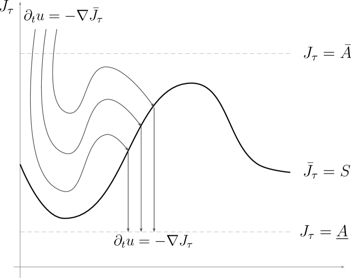
Figure 1: $(\tau)$-Yamabe and prescribed scalar curvature flows combined

Since

$$\{\partial J_{\tau}=0\}\;\cap\;\{\underline{A}\leq J_{\tau}\leq\overline{A}\}=\emptyset$$

and $J_{\tau}$ satisfies the Palais-Smale condition, as $\tau>0$, by the deformation lemma, cf. Section 7.4 in [2] and transversality for any $u\in[\underline{A}\leq J_{\tau}\leq\overline{A}]$ there exists a first time $T_{u}\geq 0$, which is continuous in $u$, such that

$$\phi(T_{u},u)\in\left\{J_{\tau}\leq\underline{A}\right\}.$$

Recalling that $\{\bar{J}_{\tau}\leq K_{\max}^{\frac{2}{p+1}}\underline{A}\}\subseteq\{J_{\tau}\leq\overline{A}\}$, consider then the homotopy

$$F:[0,1]\times(\{\bar{J}_{\tau}\leq K_{\max}^{\frac{2}{p+1}}\underline{A}\})\longrightarrow X:(s,u)\longmapsto\phi(s\,T_{u},u).$$

If $u$ belongs to the sublevel $\{J_{\tau}\leq\underline{A}\}$, then $T_{u}=0$ and hence

$$F(s,u)=u\quad\text{ for all }\quad s\in[0,1].$$

Therefore $F$ deforms $\{\bar{J}_{\tau}\leq K_{\max}^{\frac{2}{p+1}}\underline{A}\}$ into $\{J_{\tau}\leq\underline{A}\}$, but not necessarily within

$$\{\bar{J}_{\tau}\leq K_{\max}^{\frac{2}{p+1}}\underline{A}\}.$$

This can be achieved composing $\phi$ on the left with a suitable Yamabe-type flow. Recall that, if $(M^{n},g_{0})$ is Einstein and of positive Yamabe class, by Theorem 6.1 in [13] the equation

$$L_{g_{0}}u=u^{p},\quad p=\frac{n+2}{n-2}-\tau$$

has only constant solutions. Hence the infimum of $\bar{J}_{\tau}$ is attained and equal to $R_{g_{0}}Vol_{g_{0}}(M)^{1-\frac{2}{p+1}}$. Since the Palais-Smale condition holds also for $\bar{J}_{\tau}$, the gradient flow $\bar{\phi}(t,u)$ of $\bar{J}_{\tau}$ evolves all initial data $u$ to a constant function, intersecting transversally every level set of $\bar{J}_{\tau}$ higher than its infimum. Similarly to the previous reasoning there exists for any $u\in X$ a first time $\overline{T}_{u}\geq 0$, continuous in $u$, such that

$$\overline{\phi}(\overline{T}_{u},u)\in\left\{\bar{J}_{\tau}\leq K_{\max}^{\frac{2}{p+1}}\underline{A}\right\}.$$

Defining

$$\tilde{F}(s,u)=\overline{\phi}(\overline{T}_{F(s,u)},F(s,u)),$$

we deduce that $\tilde{F}(s,u)$ is a deformation retract of $\{\bar{J}_{\tau}\leq K_{\max}^{\frac{2}{p+1}}\underline{A}\}$ onto $\{J_{\tau}\leq\underline{A}\}$ and therefore realizes a homotopy equivalence, cf. Chapter II in [51].

On the other hand every non-empty sublevel $\{\bar{J}_{\tau}\leq B\}$, in particular $\{\bar{J}_{\tau}\leq K_{\max}^{\frac{2}{p+1}}\underline{A}\}$, is via the deformation lemma and Palais-Smale’s condition for $\bar{J}_{\tau}$ homotopically equivalent to a point. Hence we deduce the same property for $\{J_{\tau}\leq\underline{A}\}$. Still by the deformation lemma and the Palais-Smale condition, this is true also for $\{J_{\tau}\leq c\}$ with $c\in[\underline{A},\overline{A}]$. This concludes the proof. ∎

For the above proof to work, it is indeed sufficient to assume that the functional $J_{\tau}$ for $\tau=0$ has no critical points in a restricted energy range.

3.2 Pinching and degree counting

If problem (1.3) has no solutions, using Theorem 3 we will show that Proposition 3.1 applies, provided suitable pinching conditions on $K$ hold true. Arguing by contradiction, we will then derive existence results of which Theorem 1 is a particular case. To that end we first order the set

$$\{x_{1},\dots,x_{l}\}=\{\nabla K=0\}\cap\{\Delta K<0\}$$

so that

$$K_{1}=K(x_{1})\geq\ldots\geq K_{l}=K(x_{l}).$$

Recalling our notation in (2.9) and (2.10), for $m\in\{1,\dots,l\}$ we then define

$$\underline{E}_{m}=\hat{c}_{0}\left(\sum_{i=1}^{m}K_{i}^{\frac{2-n}{2}}\right)^{\frac{2}{n}}\quad\text{ and }\quad\overline{E}_{m}=\hat{c}_{0}\left(\sum_{i=l-m+1}^{l}K_{i}^{\frac{2-n}{2}}\right)^{\frac{2}{n}}.$$ (3.1)

As we will see, these numbers represent the minimal and maximal limit energies for solutions developing $m$ bubbles and weakly converging to zero as $\tau\longrightarrow 0$. We then have the following result.

Proposition 3.2.

Suppose that (1.3) has no solutions, and assume that

$$\left(\frac{K_{\max}}{K_{\min}}\right)^{\frac{n-2}{2}}<\frac{\underline{E}_{m+1}}{\overline{E}_{m}} \tilde{P}_{m}$$ ()

for some $m\in\{1,\dots,l-1\}$. Then there exists $0<\varepsilon\ll 1$ such that

$$\Big{\{}\partial J_{\tau}=0\Big{\}}\;\cap\;\Big{\{}(1+\varepsilon)\overline{E}_{m}\leq J_{\tau}\leq\left(\frac{K_{\max}}{K_{\min}}\right)^{\frac{2}{p+1}}(1+\varepsilon)\overline{E}_{m}\Big{\}}=\emptyset$$

for all $\tau>0$ sufficiently small.

Proof.

Suppose (1.3) has no positive solutions. Then, as $\tau\searrow 0$, all positive solutions of (1.7) with uniformly bounded energy must have zero weak limit. These are then described by Theorem 3 and of the form $u_{\tau,x_{i_{1}},\dots,x_{i_{q}}}$ with $x_{i_{1}},\dots,x_{i_{q}}$ distinct points of $\{x_{1},\dots,x_{l}\}$ and energies

$$J_{\tau}(u_{\tau,x_{i_{1}},\dots,x_{i_{q}}})\longrightarrow\hat{c}_{0}\left(\sum_{j=1}^{q}K_{i_{j}}^{\frac{2-n}{2}}\right)^{\frac{2}{n}}\quad\text{ as }\quad\tau\longrightarrow 0.$$

By the way we ordered the points $(x_{i})_{i}$, we clearly have that

$$\hat{c}_{0}\left(\sum_{j=1}^{q}K_{i_{j}}^{\frac{2-n}{2}}\right)^{\frac{2}{n}}\leq\overline{E}_{m}\quad\text{ for }\quad q\leq m$$

and

$$\hat{c}_{0}\left(\sum_{j=1}^{q}K_{i_{j}}^{\frac{2-n}{2}}\right)^{\frac{2}{n}}\geq\underline{E}_{m+1}\quad\text{ for }\quad q\geq m+1$$

Then the statement immediately follows. ∎

Remark 3.1.

Let us consider the pinching condition

$$\frac{K_{\max}}{K_{\min}}<\left(\frac{m+1}{m}\right)^{\frac{1}{n-2}}. P_{m}$$ ()

We then have

$$(P_{m+1})\;\Longrightarrow\;(P_{m})\quad\text{ and }\quad(P_{m})\;\Longrightarrow\;(\tilde{P}_{m})\quad\text{ for all }\quad m\geq 1.$$ (3.2)

Indeed, while the first implication is obvious, for the second we find from ($P_{m}$)

$$\sum_{i=1}^{m+1}K_{i}^{\frac{2-n}{2}}\geq\frac{m+1}{K_{\max}^{\frac{n-2}{2}}}>(\frac{K_{\max}}{K_{\min}})^{\frac{n-2}{2}}\frac{m}{K_{\min}^{\frac{n-2}{2}}}\geq(\frac{K_{\max}}{K_{\min}})^{\frac{n-2}{2}}\sum_{i=l-m+1}^{l}K_{i}^{\frac{2-n}{2}},$$

which implies ($\tilde{P}_{m}$) by the definitions in (3.1). Finally we observe that also

$$(\tilde{P}_{m_{1}})\;\Longrightarrow\;(\tilde{P}_{m_{2}})\quad\text{ for all }\quad m_{1}\geq m_{2}.$$ (3.3)

Indeed we may argue inductively and see that $(\tilde{P}_{m_{1}})$ for $m_{1}=m_{2}+1$ implies

$$\begin{split}\sum_{i=1}^{m_{2}+1}K_{i}^{\frac{2-n}{2}}=&\sum_{i=1}^{m_{1}+1}K_{i}^{\frac{2-n}{2}}-K_{m_{1}+1}^{\frac{2-n}{2}}>(\frac{K_{\max}}{K_{\min}})^{\frac{n-2}{2}}\sum_{i=l-m_{1}+1}^{l}K_{i}^{\frac{2-n}{2}}-K_{m_{1}+1}^{\frac{2-n}{2}}\\ =&(\frac{K_{\max}}{K_{\min}})^{\frac{n-2}{2}}\sum_{i=l-m_{2}+1}^{l}K_{i}^{\frac{2-n}{2}}+(\frac{K_{\max}}{K_{\min}})^{\frac{n-2}{2}}K_{l-m_{1}+1}^{\frac{2-n}{2}}-K_{m_{1}+1}^{\frac{2-n}{2}},\end{split}$$

and

$$(\frac{K_{\max}}{K_{\min}})^{\frac{n-2}{2}}K_{l-m_{1}+1}^{\frac{2-n}{2}}-K_{m_{1}+1}^{\frac{2-n}{2}}=K_{l-m_{1}+1}^{\frac{2-n}{2}}\left((\frac{K_{\max}}{K_{\min}})^{\frac{n-2}{2}}-(\frac{K_{l-m_{1}+1}}{K_{m_{1}+1}})^{\frac{n-2}{2}}\right)\geq 0.$$

We therefore obtain (3.3) as desired.

We prove next the following result, which by (3.2) in the previous remark extends Theorem 1.

Theorem 4.

Suppose $(M^{n},g_{0})$ is an Einstein manifold of positive Yamabe class with $n\geq 5$ and $K$ is a positive Morse function on $M$ satisfying (1.5). Assume we are in one of the following two situations:

1. $K$ satisfies $(\tilde{P}_{1})$ and (1.6);

2. $K$ satisfies $(\tilde{P}_{2})$ and has at least two critical points with negative Laplacian.

Then (1.3) has a positive solution.

Proof.

The proof will be carried out by contradiction, assuming that the functional $J_{0}$ does not have any critical point, so we have the conclusion of Proposition 3.2 and thus the conclusion of Proposition 3.1.

Suppose (j) holds: recalling (3.1), we deduce that for $\varepsilon>0$ small the sublevel $\{J_{\tau}\leq(1+\varepsilon)\overline{E}_{1}\}$ is contractible and that $J_{\tau}$ has no critical points at level $(1+\varepsilon)\overline{E}_{1}$. By Theorem 3, all critical points of $J_{\tau}$ at lower levels are single-bubbling solutions $u_{\tau,x_{i}}$, which totally contribute to the Leray-Schauder degree of (1.7) by the amount

$$\sum_{x_{j}\in\{\nabla K=0\}\cap\{\Delta K<0\}}(-1)^{n-m_{j}},$$

see (2.10). By the Poincaré-Hopf theorem this total sum must be equal to the Euler characteristic $\chi(\{J_{\tau}\leq(1+\varepsilon)\overline{E}_{1}\})=1$, which contradicts the assumption.

Suppose now that (jj) holds true, and let us again assume that $J_{0}$ has no critical points. As $(\tilde{P}_{2})$ implies $(\tilde{P}_{1})$, see Remark 3.1, we thus have a contradiction from case (j), provided (1.6) holds. Hence we may assume that $(\tilde{P}_{2})$ holds and

$$\sum_{x_{i}\in\{\nabla K=0\}\cap\{\Delta K<0\}}(-1)^{m_{i}}=(-1)^{n}.$$ (3.4)

With the same reasoning as above we obtain that for $\varepsilon>0$ small the sublevel $\{J_{\tau}\leq(1+\varepsilon)\overline{E}_{2}\}$ is contractible and that $J_{\tau}$ has no critical points at level $(1+\varepsilon)\overline{E}_{2}$.

By our assumptions solutions of (1.7) with limiting energies less or equal to $(1+\varepsilon)\overline{E}_{2}$ are either single- or doubly-bubbling solutions. By (3.4) the contribution of the former to the degree is 1, while the contribution of the latter must be zero.

By Theorem 3 doubly-bubbling solutions blow-up at distinct critical points of $K$ with negative Laplacian, whence by the characterization of their Morse index necessarily

$$0=\sum_{x_{i}\neq x_{j},x_{i},x_{j}\in\{\nabla K=0\}\cap\{\Delta K<0\}}(-1)^{n-m_{i}+n-m_{j}}.$$

Combining the last formula with (3.4), we compute

$$\begin{split}0=&\sum_{x_{i}\neq x_{j},x_{i},x_{j}\in\{\nabla K=0\}\cap\{\Delta K<0\}}(-1)^{n-m_{i}+n-m_{j}}\\ =&\sum_{x_{i}\in\{\nabla K=0\}\cap\{\Delta K<0\}}(-1)^{n-m_{i}}\sum_{x_{j}\neq x_{i},x_{j}\in\{\nabla K=0\}\cap\{\Delta K<0\}}(-1)^{n-m_{j}}\\ =&\sum_{x_{i}\in\{\nabla K=0\}\cap\{\Delta K<0\}}(-1)^{n-m_{i}}[-(-1)^{n-m_{i}}+\sum_{x_{j}\in\{\nabla K=0\}\cap\{\Delta K<0\}}(-1)^{n-m_{j}}].\end{split}$$

Using (3.4) for the latter sum, we get

$$\begin{split}0=&\sum_{x_{i}\in\{\nabla K=0\}\cap\{\Delta K<0\}}(-1)^{n-m_{i}}[-(-1)^{n-m_{i}}+1]\\ =&-\sum_{x_{i}\in\{\nabla K=0\}\cap\{\Delta K<0\}}(-1)^{2(n-m_{i})}+\sum_{x_{i}\in\{\nabla K=0\}\cap\{\Delta K<0\}}(-1)^{n-m_{i}}.\end{split}$$

Again we know that the latter sum equals $1$, consequently

$$\begin{split}0=&-\sum_{x_{i}\in\{\nabla K=0\}\cap\{\Delta K<0\}}(-1)^{2(n-m_{i})}+1=-\sharp\left(\{\nabla K=0\}\cap\{\Delta K<0\}\right)+1,\end{split}$$

where $\sharp$ denotes the cardinality. Hence we reach a contradiction once more. ∎

Remark 3.2.

1. The restriction on the dimension for condition (jj) is sharp, cf. Remark 4.1 for details. Our proof indeed relies on Theorem 3, which only holds in dimension $n\geq 5$.

2. One could replace the degree-counting argument by Morse’s inequalities. This was done in [61] in three dimensions and in [28] in arbitrary dimension under suitable pinching conditions.

3. Formula (1.6) arises from computing the contribution to the degree of all single-bubbling solutions. Considering the blowing-up solutions in Theorem 3 and the Morse-index formula there, it can be easily seen that the total degree of multi-bubbling solutions is $1$. If (1.3) is not solvable, Proposition 3.1 could then be applied for large values of $A$, since $J_{\tau}$ would have only finitely-many solutions with bounded energy, but we would derive no useful information from the Poincaré-Hopf theorem.

4. Condition (j) (resp., (jj)) is used to find sublevels of $\bar{J}_{\tau}$ that contain every blowing-up solution of (1.7) forming one bubble (resp., two bubbles) but not containing any solution forming two (resp., three) bubbles or more. Further pinching restrictions does not seem to lead to different existence results, in view of Theorem 2.

5. The argument of the proof allows to also show that the solution provided by the above theorem is a critical point of $J_{\tau}$ for $\tau=0$ below a given energy value, see the comment after Proposition 3.1. This value can be any number exceeding the limiting energy of doubly-bubbling or triply-bubbling solutions as in Theorem 3. The existence result is also stable under small perturbations of the Einstein metric and might extend to conformal classes of metrics with a unique Yamabe representative, cf. [31].

3.3 Pinching and min-max theory

Here we show how Theorem 3 can be used to improve results in the literature that rely on min-max theory, cf. [29], [22] and [63] in two dimensions or [11]. Also with this approach and under some circumstances the pinching assumption in Theorem 1 can be relaxed. We have first the following general result, which will be later specialized to simpler situations or variants.

Theorem 5.

Let $(M^{n},g)$, $n\geq 5$ be a closed Riemannian manifold of positive Yamabe class and $K$ be a positive Morse function on $M$ satisfying (1.5). Assume that there is a set $\Xi\subseteq M$ with $\mathcal{C}$ components that contains $p$ local maxima $x_{1},\dots,x_{p}$ of $K$ and such that

$$\max_{\Xi}\,(K^{\frac{2-n}{2}})<\min\left\{\left(K(x_{i})^{\frac{2-n}{2}}+K(x_{j})^{\frac{2-n}{2}}\right)^{\frac{2}{n}}\;:\;x_{i}\neq x_{j}\text{ local maxima of }K\right\}.$$

Assume also that $K$ has $q\geq 0$ critical points of index $1$ in the range

$$[\min_{\Xi}K,\max_{i\in\{1,\dots,p\}}K(x_{i})).$$

Then (1.3) has a solution provided that $q<p-\mathcal{C}$.

Remark 3.3.

Following our proof, the above result and thence the other ones in this subsection can be extended to $S^{3}$ without any pinching requirement due to single-bubbling. Note that from [41] problem (1.3) is always solvable on other three-manifolds. In four dimensions one can relax the pinching condition using constraints on multi-bubbling solutions as found in [9] and [40].

Before proving Theorem 5 we need some preliminaries. First we specify more precisely the asymptotic profile of the single-bubbling solutions $u_{\tau,x_{i}}$ as in Theorem 3. If $\varphi_{a,\lambda}$ is as in (2.7), then there exists

$$a_{i,\tau}\longrightarrow x_{i}\in\{\nabla K=0\}\cap\{\Delta K<0\}\quad\text{ and }\quad\lambda_{i,\tau}^{2}=-(1+o_{\tau}(1))c_{2}\frac{\Delta K(x_{i})}{K(x_{i})\tau}$$

as $\tau\longrightarrow 0$, where $c_{2}=c_{2}(n)>0$, see Section 3 in [49], such that

$$\left\|u_{\tau,x_{i}}-\varphi_{a_{i,\tau},\lambda_{i,\tau}}\right\|=o_{\tau}(1).$$ (3.5)

We then map $\Xi\subseteq M$ as in Theorem 5 into the variational space $X\subseteq W^{1,2}$, cf.(1.9), in such a way that each point $x_{i}$ is mapped to $u_{\tau,x_{i}}$, and derive an upper bound on $J_{\tau}$ under the image of this an embedding. Precisely consider for $r_{0}>0$ smooth

$$\tilde{\lambda}:M\longrightarrow\mathbb{R}_{+}\quad\text{ and }\quad\tilde{a}:M\longrightarrow M$$

satisfying with $a_{i,\tau}$ and $\lambda_{i,\tau}$ as in (3.5)

$$\begin{cases}\tilde{\lambda}=\tau^{-1/2}&\text{ in }\quad M\setminus\cup_{i=1}^{p}B_{4r_{0}}(x_{i});\\ \tilde{\lambda}=\lambda_{i,\tau}&\text{ in }\quad B_{2r_{0}}(x_{i})\\ c\tau^{-1/2}\leq\tilde{\lambda}\leq C\tau^{-1/2}&\text{ in }\quad M\end{cases}$$

and

$$\begin{cases}\tilde{a}(x)=x&\text{ in }\quad M\setminus\cup_{i=1}^{p}B_{4r_{0}}(x_{i});\\ \tilde{a}(x)=a_{i,\tau}&\text{ in }\quad B_{2r_{0}}(x_{i});\\ \tilde{a}\in B_{4r_{0}}(x_{i})&\text{ in }\quad B_{4r_{0}}(x_{i})\end{cases}$$

for some fixed constants $0<c<C$. Finally let for $x\in\Xi$

$$\tilde{\varphi}_{x,\tau}=\begin{cases}\varphi_{\tilde{a}(x),\tilde{\lambda}(x)}&\text{ in }\quad M\setminus\cup_{i=1}^{p}B_{2r_{0}}(x_{i});\\ (1-\frac{d(x,x_{i})}{2r_{0}})u_{\tau,x_{i}}+\frac{d(x,x_{i})}{2r_{0}}\varphi_{a_{i,\tau},\lambda_{i,\tau}}&\text{ in }\quad B_{2r_{0}}(x_{i}).\end{cases}$$ (3.6)

We then have the following result.

Lemma 3.1.

If $\tilde{\varphi}_{x,\tau}$ is as in (3.6) and if $\hat{c}_{0}$ is given in (2.9), one has that

$$\sup_{x\in\Xi}J_{\tau}(\tilde{\varphi}_{x,\tau}/\|\tilde{\varphi}_{x,\tau}\|)\leq\hat{c}_{0}\max_{\Xi}\,(K^{\frac{2-n}{2}})+o_{\tau}(1)+o_{r_{0}}(1),$$

where $o_{\tau}(1)\longrightarrow 0$ as $\tau\searrow 0$ and $o_{r_{0}}(1)\xrightarrow{r_{0}\to 0}0$.

Proof.

Since $J_{\tau}$ is uniformly Lipschitz on finite energy sublevels and is scaling invariant, by (3.5) we are reduced to prove that

$$J_{\tau}({\varphi}_{x,\tilde{\lambda}(x)})\leq\hat{c}_{0}K(x)^{\frac{2-n}{n}}+o_{\tau}(1)\quad\text{ as }\quad\tau\searrow 0.$$

To show this, note that $\varphi_{x,\tilde{\lambda}(x)}$ is bounded from above and below by powers of

$$\tilde{\lambda}(x)\simeq\tau^{-1/2},$$

and that $\tilde{\lambda}(x)^{\tau}\longrightarrow 1$ as $\tau\longrightarrow 0$, whence

$$J_{\tau}({\varphi}_{x,\tilde{\lambda}(x)})=\frac{\int_{M}\left(c_{n}|\nabla{\varphi}_{x,\tilde{\lambda}(x)}|_{g_{0}}^{2}+R_{g_{0}}{\varphi}_{x,\tilde{\lambda}(x)}^{2}\right)d\mu_{g_{0}}}{(\int_{M}K{\varphi}_{x,\tilde{\lambda}(x)}^{2^{*}}d\mu_{g_{0}})^{\frac{2}{2^{*}}}}+o_{\tau}(1),\quad 2^{*}=\frac{2n}{n-2}.$$

Using a change of variables, it is easy to see that

$$\begin{split}\frac{\int_{M}\left(c_{n}|\nabla{\varphi}_{x,\tilde{\lambda}(x)}|_{g_{0}}^{2}+R_{g_{0}}{\varphi}_{x,\tilde{\lambda}(x)}^{2}\right)d\mu_{g_{0}}}{(\int_{M}K{\varphi}_{x,\tilde{\lambda}(x)}^{2^{*}}d\mu_{g_{0}})^{\frac{2}{2^{*}}}}=&c_{n}K(x)^{\frac{2-n}{n}}\frac{\int_{\mathbb{R}^{n}}|\nabla U_{0}|^{2}dx}{\left(\int_{\mathbb{R}^{n}}|U_{0}|^{2^{*}}dx\right)^{\frac{2}{2^{*}}}}+o_{\tau}(1)\\ =&\hat{c}_{0}K(x)^{\frac{2-n}{n}}+o_{\tau}(1),\end{split}$$

where $U_{0}$ is given by (2.8). This concludes the proof. ∎

Proof.

of Theorem 5. Arguing by contradiction, assume that (1.3) has no solutions. Then, as noticed in the previous subsection, all solutions of (1.7) with uniformly bounded energy must have zero weak limit. Fix $\varepsilon>0$ small: we know by Theorem 3 that $J_{\tau}$ has at least $p$ local minima of the form $u_{\tau,x_{1}},\dots,u_{\tau,x_{p}}$ such that for $\tau$ small there holds

$$J_{\tau}(u_{\tau,x_{j}})<\hat{c}_{0}(\min_{i\in\{1,\dots,p\}}K(x_{i}))^{\frac{2-n}{n}}+\varepsilon$$

and such that, for all sufficiently small values of $\tau$, $J_{\tau}$ has no critical point at level

$$\hat{c}_{0}(\min_{i\in\{1,\dots,p\}}K(x_{i}))^{\frac{2-n}{n}}+\varepsilon.$$

We can assume that for $\tau$ small there is no critical point of $J_{\tau}$ at level

$$\hat{c}_{0}\max_{\Xi}\,(K^{\frac{2-n}{2}})+\varepsilon$$

and we can modify $J_{\tau}$ near all its local minima at level less or equal to

$$\hat{c}_{0}\max_{\Xi}\,(K^{\frac{2-n}{2}})+\varepsilon,$$

which are non-degenerate by Theorem 3, in order to still have the Palais-Smale condition, to not generate new critical points and so that the modified minima are at level zero. Call $\tilde{J}_{\tau}$ the resulting functional, which we can take of class $C^{2,\alpha}$ as the original one, see Figure 2. It will also possess at least $p$ critical points at level zero.

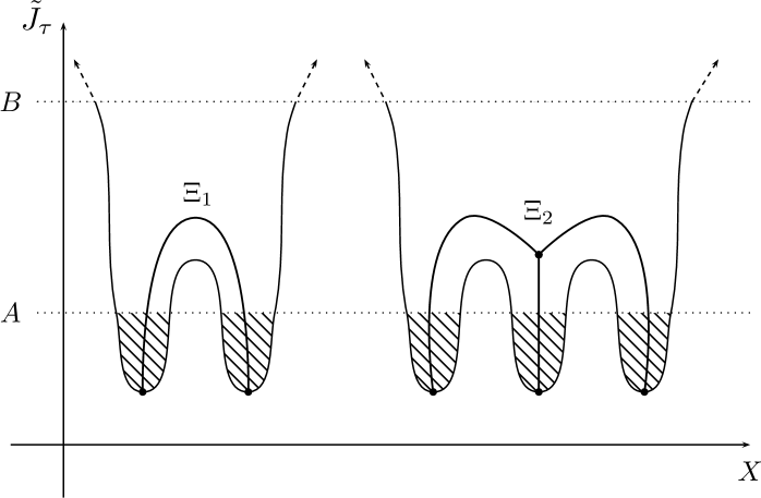
Figure 2: The modified functional $\tilde{J}_{\tau}$ and its sublevels.

We then use relative Morse inequalities for $\tilde{J}_{\tau}$, cf. Theorem 4.3 in [18], between the levels

$$A=\varepsilon\quad\text{ and }\quad B=\hat{c}_{0}\max_{\Xi}\,(K^{\frac{2-n}{2}})+\varepsilon.$$

By construction $\tilde{J}_{\tau}$ has $C_{0}=0$ critical points of index zero and $C_{1}=q$ critical points in the range $[A,B]$. Since $\tilde{J}_{\tau}$ has no local minima in the range $[A,B]$ and the Palais-Smale condition holds true, every point of $\{\tilde{J}_{\tau}\leq B\}$ can be joined to $\{\tilde{J}_{\tau}\leq A\}$. As a consequence

$$\beta_{0}:=\text{rank}\,H_{0}(\{\tilde{J}_{\tau}\leq B\},\{\tilde{J}_{\tau}\leq A\})=0,$$

see e.g. [34], Chapter 2, Exercise 16, page 130. On the other hand consider

$$\beta_{1}:=\text{rank}\,H_{1}(\{\tilde{J}_{\tau}\leq B\},\{\tilde{J}_{\tau}\leq A\}).$$

Recall that

$$H_{1}(\{\tilde{J}_{\tau}\leq B\},\{\tilde{J}_{\tau}\leq A\})=Z_{1}(\{\tilde{J}_{\tau}\leq B\},\{\tilde{J}_{\tau}\leq A\})/B_{1}(\{\tilde{J}_{\tau}\leq B\},\{\tilde{J}_{\tau}\leq A\}),$$

where $Z_{1}$ and $B_{1}$ denote kernel and image of the boundary operators in one and two homological dimensions respectively, cf. [51], Chapter VII, §6. We claim next

$$\beta_{1}\geq p-\mathcal{C}.$$ (3.7)

To prove this, let $\Xi_{1},\dots,\Xi_{\mathcal{C}}$ denote the connected components of $\Xi$. As our assumptions improve or stay invariant if we remove components containing none or only one point among $x_{1},\dots,x_{p}$, we can assume that each component of $\Xi$ contains at least two among the points $x_{1},\dots,x_{p}$.

Given $\Xi_{j}$ let

$$X_{j}=\{x_{i_{1}},\dots x_{i_{\mathcal{C}_{j}}}\}$$

denote the local maxima of $K$ belonging to $\Xi_{j}$. Considering a curve

$$\gamma_{j,l}:[0,1]\longrightarrow M\quad\text{ with }\quad\gamma(0)=x_{i_{1}}\quad\text{ and }\quad\gamma(1)=x_{i_{l}}\quad\text{ for }\quad l=2,\dots,i_{\mathcal{C}_{j}}$$

its image is a one-chain in $Z_{1}(\{\tilde{J}_{\tau}\leq B\},\{\tilde{J}_{\tau}\leq A\})$ with boundary

$$x_{i_{l}}-x_{i_{1}}\in C_{0}(\{\tilde{J}_{\tau}\leq A\}).$$

It turns out that

$$\gamma_{j,2},\dots,\gamma_{j,\mathcal{C}_{j}}\quad\text{ generate }\mathcal{C}_{j}-1\text{ elements of }\quad H_{1}(\{\tilde{J}_{\tau}\leq B\},\{\tilde{J}_{\tau}\leq A\}),$$ (3.8)

which are linearly independent. To prove (3.7) we show that any

$$\sum_{2\leq h\leq\mathcal{C}_{j}}n_{h}\gamma_{j,h}$$

with not all $n_{h}=0$ cannot be written as

$$\sum_{2\leq h\leq\mathcal{C}_{j}}n_{h}\gamma_{j,h}=\partial_{2}\mathfrak{c}_{2}+\mathfrak{c}_{1}$$ (3.9)

with $\mathfrak{c}_{2}\in C_{2}(\{\tilde{J}_{\tau}\leq B\},\{\tilde{J}_{\tau}\leq A\})$ and $\mathfrak{c}_{1}\in C_{1}(\{\tilde{J}_{\tau}\leq A\}).$

In fact let us apply the boundary operator $\partial_{1}$ to both sides of the latter equation. As not all $n_{h}$ are zero, $\partial_{1}\left(\sum_{h}n_{h}\gamma_{j,h}\right)$ is non-trivial in $C_{0}(\{\tilde{J}_{\tau}\leq A\})$. Clearly $\partial_{1}\circ\partial_{2}=0$, so to achieve (3.9) we would need $\partial_{1}\mathfrak{c}_{1}$ to be in $C_{0}(\{\tilde{J}_{\tau}\leq A\})$ a non-trivial linear combination of the points $x_{i_{1}},\dots,x_{i_{l}}$. However, since $x_{i_{1}},\dots,x_{i_{l}}$ lie in different components of $\{\tilde{J}_{\tau}\leq A\}$, there is no chain $\mathfrak{c}_{1}\in C_{1}(\{\tilde{J}_{\tau}\leq A\})$ with this property. This shows (3.8). Repeating this reasoning for every component of $\Xi$ we obtain

$$\beta_{1}\geq\sum_{j=1}^{\mathcal{C}}(\mathcal{C}_{j}-1)=p-\mathcal{C},$$

since $\sum_{j=1}^{\mathcal{C}}\mathcal{C}_{j}=p$. This shows (3.7). Now the relative Morse inequalities imply

$$q=C_{1}=C_{1}-C_{0}\geq\beta_{1}-\beta_{0}\geq p-\mathcal{C},$$

contradicting our assumptions. ∎

In some particular cases we obtain the following corollary, cf. Theorem 1 (ii).

Corollary 3.1.

Suppose that $K$ satisfies $\frac{K_{\max}}{K_{\min}}\leq 2^{\frac{2}{n-2}}$, that it has $p$ local maxima and $q$ critical points of index $n-1$ with negative Laplacian. Then (1.3) admits a positive solution provided $q<p-1$.

Proof.

In the theorem choose the connected set $\Xi=S^{n}$, see (3.1), (3.2). ∎

We next state a related result, proved with similar techniques.

Theorem 6.

Let $(M,g)$ be as in Theorem 5. Suppose $K$ has a local maximum point $z$, and that there exists a curve $a(t)$ joining $z$ to another point $y$ with

$$K(y)\geq K(z)$$

such that both the following two properties hold

1. for all $x_{i}\neq x_{j}$ local maxima of $K$

   $$\max_{t}K(a(t))^{\frac{2-n}{n}}<\left(K(x_{i})^{\frac{2-n}{2}}+K(x_{j})^{\frac{2-n}{2}}\right)^{\frac{2}{n}}\};$$

2. critical points of index $n-1$ in the range

   $$[\min_{t}K(a(t)),K(z)]$$

   have positive Laplacian.

Then (1.3) has a positive solution.

Proof.

We can construct a curve $\tilde{a}(t)$ joining $y$ to another maximum point $\tilde{z}$ of $K$ and such that $\min_{t}K(\tilde{a}(t))=K(y)$. Consider then the composition $\hat{a}:=a*\tilde{a}$, and the test functions $\tilde{\varphi}_{x,\tau}$ as in (3.6) for $x$ in the image of the curve $\hat{a}$. By Lemma 3.1 and construction of $\hat{a}$, we have that the image of this curve in $X$ connects two strict local minima $u_{\tau,z}$, $u_{\tau,\tilde{z}}$ of $J_{\tau}$, and the supremum of $J_{\tau}$ on the image is bounded above by

$$\hat{c}_{0}(\min_{t\in[0,1]}K(a(t)))^{\frac{2-n}{n}}+o_{\tau}(1)+o_{r_{0}}(1).$$

Consider a mountain-pass path between the strict local minima $u_{\tau,z}$, $u_{\tau,\tilde{z}}$ of $J_{\tau}$. Assuming that (1.3) has no solutions, by the Palais-Smale condition for $J_{\tau}$ and by the fact that all critical points with uniformly bounded energy of $J_{\tau}$ as described in Theorem 3 are non-degenerate, $J_{\tau}$ must possess a critical point of index one at a level less or equal to

$$\hat{c}_{0}(\min_{t\in[0,1]}K(a(t)))^{\frac{2-n}{n}}+o_{\tau}(1)+o_{r_{0}}(1).$$

Still by Theorem 3 and condition (i) this critical point must have a simple blow-up at a critical point $p$ of $K$ of index $n-1$ with

$$K(p)\in[\min_{t}K(a(t)),K(z)],$$

which is excluded by assumption (ii). ∎

Remark 3.4.

The latter result improves the pinching condition of Theorem 2 in [11] (if compactified from $\mathbb{R}^{n}$ to $S^{n}$) for $K$ Morse and satisfying (1.5), namely

1. $K_{\max}<2^{\frac{2}{n-2}}\min_{t}K(x(t))$;

2. critical points in the range $[\min_{t}K(x(t)),K(z))$ are local maxima or have positive Laplacian.

While the strategy in [11] might be possibly used to relax condition (jj), an improvement of (j) requires a more careful analysis of the loss of compactness, as done in [48] and [53].

4 Non-existence results

In this section we prove non-existence results on $S^{n}$ for arbitrarily pinched curvature candidates of prescribed Morse type and with only one critical point with negative Laplacian. We show that the assumptions of Theorem 1 are sharp both in terms of Morse structure and dimension, cf. Remark 4.1.

We construct a sequence of functions $(K_{m})_{m}$ on $S^{n}$ with only one local maximum, while all other critical points have positive Laplacian and converge to the south pole. We build the $(K_{m})_{m}$ in order to preserve a given Morse structure and to maintain uniform $C^{3}$ bounds.

We denote by $\mathtt{y}_{i}$ for $i=1,\dots,n+1$ the Euclidean coordinate functions on $\mathbb{R}^{n+1}$ restricted to $S^{n}$ and by $\mathtt{N},\mathtt{S}$ the north and south poles respectively, i.e.

$$\mathtt{N}=S^{n}\cap\{\mathtt{y}_{n+1}=1\}\quad\text{ and }\quad\mathtt{S}=S^{n}\cap\{\mathtt{y}_{n+1}=-1\}.$$

Finally we let

$$\pi_{\mathtt{N}}:S^{n}\setminus\{\mathtt{N}\}\longrightarrow\mathbb{R}^{n}\quad\text{ and }\quad\pi_{\mathtt{S}}:S^{n}\setminus\{\mathtt{S}\}\longrightarrow\mathbb{R}^{n}$$

denote the stereographic projections from the $\mathtt{N},\mathtt{S}$, whose inverse $\pi_{\mathtt{N}}^{-},\pi_{\mathtt{S}}^{-}$ induce coordinate systems on $S^{n}\setminus\{\mathtt{N}\},S^{n}\setminus\{\mathtt{S}\}$, to which we will refer as $\pi_{\mathtt{N}}$ and $\pi_{\mathtt{S}}$ coordinates respectively.

Recalling our notation in (1.10) we have the next result, proved in the Appendix.

Proposition 4.1.

For every Morse function $\tilde{K}:S^{n}\longrightarrow\mathbb{R}$ with only one local maximum point there exists a sequence of positive functions $(K_{m})_{m}$ such that

1. $\mathcal{M}_{j}(K_{m})=\mathcal{M}_{j}(\tilde{K})$ for all $j=0,\dots,n$ and $K_{m}$ has only one local maximum point at $\mathtt{N}$, while all other critical points of $K_{m}$ converge to $\mathtt{S}$;

2. there exists a neighbourhood $U\subseteq S^{n}$ of $\mathtt{S}$ and $c>0$ such that

   $$\Delta K_{m}\geq c\quad\text{ on }\quad U;$$

3. $K_{m}\longrightarrow K_{0}$ in $C^{3}(S^{n})$, where $K_{0}$ is a positive monotone non-decreasing function in $\mathtt{y}_{n+1}$, affine and non-constant in $\mathtt{y}_{n+1}$ outside of a small neighbourhood of $\mathtt{S}$.

4.1 Uniform bounds away from the poles

We consider the sequence $(K_{m})_{m}$ given by Proposition 4.1 and a sequence of positive solutions to

$$L_{g_{S^{n}}}u_{m}=K_{m}u_{m}^{\frac{n+2}{n-2}}\quad\text{ on }\quad(S^{n},g_{S^{n}}).$$ (4.1)

Even without assuming uniform energy bounds as in Theorem 3, we aim to prove that $(u_{m})_{m}$ stays uniformly bounded on compact sets of $S^{n}\setminus\{\mathtt{N}\}$.

By construction, see the first and final steps in the proof of Proposition 4.1, the only critical points of $K_{0}$ are $\mathtt{N}$ and a compact set $K_{U}\subseteq U$, where the Laplacian is positive and bounded away from zero. By Corollary 1.4 in [24] or Theorem 2 in [30] the sequence $(u_{m})_{m}$ is uniformly bounded in $L^{\infty}$ on compact sets of

$$S^{n}\setminus\{\mathtt{N}\cup K_{U}\},$$

since $|\nabla K_{m}|$ is bounded away from zero here, hence we only need to focus on $K_{U}$.

For doing this, we cannot directly use known results in the literature due to the degenerating behaviour of $(K_{m})_{m}$. However, the proof can be obtained combining the preliminary results in Subsection 2.3. It will be harder to understand the blow-up behaviour near the north pole $\mathtt{N}$. Before proceeding recall Definition 2.1.

Lemma 4.1.

Suppose $(u_{m})_{m}$ solves (4.1). Then the blow-up points in $U$ are isolated simple.

Proof.

The proof uses also some argument in Section 8 of [45], but we have here variable curvature. For $0<\delta\ll 0$ and $R\gg 1$ let $\xi_{1,m},\dots\xi_{N(u_{m}),m}$ be the points given by Proposition 2.1. As $(u_{m})_{m}$ is uniformly bounded away from $\{\mathtt{N}\}\cup K_{U}$, all $\xi_{i,m}$ will lie in a neighbourhood of $\{\mathtt{N}\}\cup K_{U}$. Let us denote by

$$\xi_{1,m},\dots,\xi_{N_{m},m}\quad\text{ with }\quad N_{m}\leq N(u_{m})$$

the points contained in a neighbourhood of $K_{U}$.

We may assume that with $c_{n}$ as in (1.1) and in $\pi_{\mathtt{N}}$ coordinates $u_{m}$ solves

$$-c_{n}\Delta u_{m}=K_{m}u_{m}^{\frac{n+2}{n-2}}\quad\text{ in }\quad B_{1}(0),$$ (4.2)

where and we identify $K_{m}$ with $K_{m}\circ\pi_{\mathtt{N}}^{-}$. For any $m$ we choose $i\neq j$ such that

$$|\xi_{i,m}-\xi_{j,m}|=\min\{|\xi_{k,m}-\xi_{l,m}|\>:\;k,l\in\{1,\dots N_{m}\},k\neq l\}.$$ (4.3)

We let $\xi_{m}=\xi_{i,m}$, $s_{m}=\frac{1}{2}|\xi_{i,m}-\xi_{j,m}|$ and consider

$$\zeta_{m}(x)=s_{m}^{\frac{n-2}{2}}u_{m}\left(s_{m}x+\xi_{m}\right).$$ (4.4)

By definition of $s_{m}$ and (iii) in Proposition 2.1 the sequence $(\zeta_{m})_{m}$ has an isolated blow-up at zero. We will prove next that this blow-up is indeed also isolated simple.

First, using the classification result in [15], it is standard to show that there exists $R_{m}\longrightarrow\infty$ sufficiently slowly such that

$$\left\|\zeta_{m}(0)^{-1}\zeta_{m}\left(\zeta_{m}(0)^{-\frac{2}{n-2}}\cdot\right)-\left(1+k_{m}|\cdot|^{2}\right)^{\frac{2-n}{2}}\right\|_{C^{2}(B_{R_{m}}(\xi_{m}))}\longrightarrow 0,$$ (4.5)

where $k_{m}=\frac{1}{n(n-2)c_{n}}K_{m}(\xi_{m})$, cf. Proposition 2.1 in [39].

Assuming by contradiction that the blow-up of $\zeta_{m}$ at $0$ is not isolated simple, let $\overline{w}_{m}$ be as in (2.16) replacing $\overline{u}_{m}$ by $\overline{\zeta}_{m}$. By (4.5) then $\overline{w}_{m}$ has a first critical point for $r$ of order $\overline{\zeta}_{m}(0)^{-\frac{2}{n-2}}$ and, if the blow-up of $\zeta_{m}$ is not isolated simple,

$$\tilde{s}_{m}=\inf\{s>R_{m}\zeta_{m}(0)^{-\frac{2}{n-2}}\;:\;\overline{w}^{\prime}_{m}(s)=0\}$$

is well defined and $\tilde{s}_{m}\ll 1$. If we let $\tilde{\zeta}_{m}(x)=\tilde{s}_{m}^{\frac{n-2}{2}}\zeta_{m}\left(\tilde{s}_{m}x\right)$, then $\tilde{\zeta}_{m}$ satisfies

$$-c_{n}\Delta\tilde{\zeta}_{m}=\tilde{K}_{m}(x)\tilde{\zeta}_{m}^{\frac{n+2}{n-2}};\qquad\tilde{K}_{m}(x)=K_{m}(\xi_{m}+\hat{s}_{m}x),\quad\hat{s}_{m}=s_{m}\tilde{s}_{m},$$ (4.6)

and has an isolated blow-up at zero. From Lemma 2.2 we deduce

$$\tilde{\zeta}_{m}(0)\tilde{\zeta}_{m}(x)\longrightarrow a|x|^{2-n}+h(x)\geq 0\quad\text{ in }\quad C^{2}_{\text{loc}}(\mathbb{R}^{n}\setminus\{0\}),$$

where $h$ is harmonic on $\mathbb{R}^{n}$ and $a>0$. By the first observation after Lemma 2.2 the function $h$ must be constant, and passing to the limit for the condition $\overline{w}^{\prime}_{m}(\tilde{s}_{m})=0$ one finds that $h\equiv a>0$, as for (3.4) in [39].

From Lemma 2.2 and, since $\tilde{\zeta}_{m}$ has an isolated simple blow-up, it follows that

$$\tilde{\zeta}_{m}(x)\leq C\tilde{\zeta}_{m}(0)^{-1}|x|^{2-n}\quad\text{ for }\quad|x|\in[R_{m}\tilde{\zeta}_{m}(0)^{-\frac{2}{n-2}},1].$$ (4.7)

For $\delta>0$ fixed, we now let $B_{\delta}:=B_{\delta}(0)$, and for all $i=1,\dots,n$ we clearly have

$$\begin{split}\frac{1}{2^{*}}\int_{B_{\delta}}\frac{\partial\tilde{K}_{m}}{\partial x_{i}}\tilde{\zeta}_{m}^{2^{*}}dx=&\frac{1}{2^{*}}\int_{B_{\delta}}\frac{\partial\tilde{K}_{m}}{\partial x_{i}}(0)\tilde{\zeta}_{m}^{2^{*}}dx\\ &+\frac{1}{2^{*}}\int_{B_{\delta}}\left(\frac{\partial\tilde{K}_{m}}{\partial x_{i}}-\frac{\partial\tilde{K}_{m}}{\partial x_{i}}(0)\right)\tilde{\zeta}_{m}^{2^{*}}dx.\end{split}$$ (4.8)

By the uniform $C^{3}$-bounds on $(K_{m})$, see Proposition 4.1, the convergence in (4.5), the upper bound in (4.7), a cancellation by oddness and a change of variables we find that the last term in (4.8) is of order $o(\hat{s}_{m}\tilde{\zeta}_{m}(0)^{-\frac{2}{n-2}})$, so

$$\frac{1}{2^{*}}\int_{B_{\delta}}\frac{\partial\tilde{K}_{m}}{\partial x_{i}}(0)\tilde{\zeta}_{m}^{2^{*}}dx=\frac{1}{2^{*}}\int_{B_{\delta}}\frac{\partial\tilde{K}_{m}}{\partial x_{i}}\tilde{\zeta}_{m}^{2^{*}}dx+o(\hat{s}_{m}\tilde{\zeta}_{m}(0)^{-\frac{2}{n-2}}).$$

By elliptic regularity theory the upper bound (4.7) implies

$$|\nabla\tilde{\zeta}_{m}(x)|\leq C\tilde{\zeta}_{m}(0)^{-1}\quad\text{ on }\quad\partial B_{\delta}.$$

Therefore, from (2.14) we deduce

$$\frac{1}{2^{*}}\int_{B_{\delta}}\frac{\partial\tilde{K}_{m}}{\partial x_{i}}\tilde{\zeta}_{m}^{2^{*}}dx=\oint_{\partial B_{\delta}}O(\tilde{\zeta}_{m}^{2^{*}}+|\nabla\tilde{\zeta}_{m}|^{2})d\sigma=O_{\delta}(\tilde{\zeta}_{m}(0)^{-2}).$$

It follows from the last two formulas that

$$\frac{\partial\tilde{K}_{m}}{\partial x_{i}}(0)=O_{\delta}(\tilde{\zeta}_{m}(0)^{-2})+o(\hat{s}_{m}\tilde{\zeta}_{m}(0)^{-\frac{2}{n-2}}).$$ (4.9)

We next rewrite (2.12) for $\tilde{\zeta}_{m}$ as

$$\begin{split}\frac{1}{2^{*}}\int_{B_{\delta}}\sum_{i}x_{i}&\frac{\partial\tilde{K}_{m}}{\partial x_{i}}(0)\tilde{\zeta}_{m}^{2^{*}}dx+\frac{1}{2^{*}}\int_{B_{\delta}}\sum_{i}x_{i}\left(\frac{\partial\tilde{K}_{m}}{\partial x_{i}}-\frac{\partial\tilde{K}_{m}}{\partial x_{i}}(0)\right)\tilde{\zeta}_{m}^{2^{*}}dx\\ &-\frac{1}{2\cdot 2^{*}}\oint_{\partial B_{\delta}}\tilde{K}_{m}\tilde{\zeta}_{m}^{2^{*}}d\sigma=c_{n}\oint_{\partial B_{\delta}}B(1/2,x,\tilde{\zeta}_{m},\nabla\tilde{\zeta}_{m})d\sigma.\end{split}$$ (4.10)

Using the same reasoning as after (4.8), one finds that

$$\int_{B_{\delta}}x_{i}\tilde{\zeta}_{m}^{2^{*}}dx=o(\tilde{\zeta}_{m}(0)^{-\frac{2}{n-2}}).$$

From these formulas and (4.9) we then deduce that

$$\int_{B_{\delta}}\sum_{i}x_{i}\frac{\partial\tilde{K}_{m}}{\partial x_{i}}(0)\tilde{\zeta}_{m}^{2^{*}}dx=o_{\delta}(\tilde{\zeta}_{m}(0)^{-\frac{2(n-1)}{n-2}})+o(\hat{s}_{m}\tilde{\zeta}_{m}(0)^{-\frac{4}{n-2}}).$$ (4.11)

Still using the uniform $C^{3}$-bounds on $(K_{m})$, the convergence in (4.5), the upper bound in (4.8) and a change of variables we find that with some $l_{n}>0$

$$\int_{B_{\delta}}\sum_{i}x_{i}\left(\frac{\partial\tilde{K}_{m}}{\partial x_{i}}-\frac{\partial\tilde{K}_{m}}{\partial x_{i}}(0)\right)\tilde{\zeta}_{m}^{2^{*}}dx=l_{n}\hat{s}_{m}(\Delta K_{m}(\xi_{m})+o_{m}(1))\tilde{\zeta}_{m}(0)^{-\frac{4}{n-2}}.$$ (4.12)

Moreover, since $\tilde{\zeta}_{m}(x)\leq C\tilde{\zeta}_{m}(0)^{-1}|x|^{2-n}$ on $\partial B_{\delta}$, we have

$$\frac{1}{2\cdot 2^{*}}\oint_{\partial B_{\delta}}\tilde{K}_{m}\tilde{\zeta}_{m}^{2^{*}}d\sigma=O_{\delta}(\tilde{\zeta}_{m}(0)^{-2^{*}}),$$

so recalling (2.19) we get from (4.10) and the latter estimates that, for $\delta$ small

$$\begin{split}\frac{l_{n}}{2^{*}}\hat{s}_{m}(\Delta K_{m}(\xi_{m})&+o_{m}(1))\tilde{\zeta}_{m}(0)^{-\frac{4}{n-2}}\\ &+\frac{(n-2)^{2}}{2}h(0)\omega_{n}\frac{c_{n}+o_{m}(1)}{\tilde{\zeta}_{m}(0)^{2}}=o_{\delta}(\tilde{\zeta}_{m}(0)^{-\frac{2(n-1)}{n-2}}),\end{split}$$

a contradiction to $h(0)=a>0$ and the fact that $\Delta K_{m}(\xi_{m})$ is positively bounded away from zero. We hence proved that $\zeta_{m}$ has an isolated simple blow-up at zero.

The exactly same strategy, but using the second observation after Lemma 2.2, then shows

$$2s_{m}=|\xi_{i,m}-\xi_{j,m}|\not\to 0\quad\text{ as }\quad m\longrightarrow\infty,$$ (4.13)

as for Section 8 in [45], proving that the blow-ups of $u_{m}$ in $U$ are isolated. Repeating once more the argument used above for $\tilde{\zeta}_{m}$ shows that the blow-ups of $u_{m}$ in $U$ are indeed also isolated simple, which is the desired result. ∎

Proposition 4.2.

For $(K_{m})_{m}$ given by Proposition 4.1 let $u_{m}$ solve (4.1) with $n\geq 5$. Then $(u_{m})_{m}$ is uniformly bounded on the compact sets of $S^{n}\setminus\{\mathtt{N}\}$.

Proof.

Using the notation in the previous proof, it is sufficient to prove that no blow-up occurs at points in $K_{U}$. We know by Lemma 4.1 that such blow-ups would be isolated simple and therefore they could be at most finitely-many. Let $\xi_{m}\longrightarrow\xi_{U}$ be a blow-up point in $K_{U}$. Then by Lemma 2.2 and the Harnack inequality we find that in $\pi_{\mathtt{N}}$ coordinates

$$u_{m}(\xi_{m})u_{m}(x+\xi_{m})\longrightarrow a|x|^{2-n}+h(x)\quad\text{ in }\quad C^{2}_{\text{loc}}(\mathbb{R}^{n}\setminus S),$$

where $S$ is a finite set, $a>0$ and $h$ harmonic near $0\in S$. Moreover $h(0)\geq 0$, see the comments after Lemma 2.2. By Lemma 2.2 there exists some fixed $r>0$ so that the upper bound (2.18) holds on $\partial B_{r/2}(0)$. Hence and by (2.19) we obtain

$$\frac{r}{2}\oint_{\partial B_{r/2}(\xi_{m})}K_{m}u_{m}^{2^{*}}d\sigma=\frac{O(1)}{u_{m}(\xi_{m})^{2^{*}}}$$

and

$$\oint_{\partial B_{r/2}(\xi_{m})}B(r/2,x,u_{m},\nabla u_{m})d\sigma\leq\frac{o_{m}(1)}{u_{m}(\xi_{m})^{2}}.$$

Moreover, reasoning as for (4.11) and (4.12), but on a ball of fixed radius, we find that for some $l_{n}>0$

$$\int_{B_{r/2}(\xi_{m})}\sum_{i}x_{i}\frac{\partial K_{m}}{\partial x_{i}}u_{m}^{2^{*}}dx=\frac{l_{n}\Delta K_{m}(\xi_{m})+o_{m}(1)}{u_{m}(\xi_{m})^{\frac{4}{n-2}}},$$

which immediately leads to a contradiction to (2.12), since $n\geq 5$ and

$$\Delta K_{m}(\xi_{m})\geq c/2>0.$$

This concludes the proof. ∎

4.2 Conclusion

Here we prove our non-existence result, Theorem 2, showing that sequences of solutions to (4.1) can neither have a non-zero limit nor develop blow-ups, which is impossible.

Lemma 4.2.

Let $K_{0}$ be a monotone function as in Proposition 4.1. Then neither

$$L_{g_{S^{n}}}u=K_{0}u^{\frac{n+2}{n-2}}\quad\text{ on }\quad S^{n},$$ (4.14)

nor

$$L_{g_{S^{n}}}u=K_{0}u^{\frac{n+2}{n-2}}\quad\text{ on }\quad S^{n}\setminus\{\mathtt{N}\}$$ (4.15)

admits positive solutions.

Proof.

Non existence for (4.14) simply follows from the Kazdan-Warner obstruction. Arguing by contradiction for (4.15), we obtain in $\pi_{\mathtt{S}}$ coordinates and by conformal invariance of the equation a positive solution $u$ of the problem

$$-c_{n}\Delta u=K_{0}u^{\frac{n+2}{n-2}}\quad\text{ in }\quad\mathbb{R}^{n}\setminus\{0\},$$ (4.16)

where we are identifying $K_{0}$ with $K_{0}\circ\pi_{\mathtt{S}}^{-1}$, which is radially non-increasing and somewhere strictly decreasing. Since the solution of (4.15) is smooth near $\mathtt{S}$, the solution $u$ of (4.16) satisfies

$$u(x)\leq C|x|^{2-n}\quad\text{ and }\quad|\nabla u(x)|\leq C|x|^{1-n}\quad\text{ for }\quad|x|\longrightarrow\infty$$ (4.17)

for some positive and fixed constant $C$. Let us write the Pohozaev identity in the complement of a ball, i.e. on

$$A_{\varepsilon}:=\mathbb{R}^{n}\setminus B_{\varepsilon}(0).$$

By (4.17) no boundary terms at infinity are involved, whence

$$\frac{1}{2^{*}}\int_{A_{\varepsilon}}u^{2^{*}}\sum_{i}x_{i}\frac{\partial K_{0}}{\partial x_{i}}\,dx=\frac{1}{2^{*}}\oint_{\partial A_{\varepsilon}}\langle x,\nu\rangle K_{0}u^{2^{*}}d\sigma+c_{n}\oint_{\partial A_{\varepsilon}}B(\varepsilon,x,u,\nabla u)\,d\sigma,$$ (4.18)

see (2.12) and the subsequent formula. By Theorem 1.1 in [67]

$$\;\exists\;C>0\;:\;u(x)\leq C|x|^{\frac{2-n}{2}}\quad\text{ as }\quad 0\neq x\longrightarrow 0.$$ (4.19)

We now consider two cases.

Case 1. There exists $C>0$ such that

$$C^{-1}|x|^{\frac{2-n}{2}}\leq u(x)\quad\text{ as }\quad 0\neq x\longrightarrow 0.$$

In this case there exists by Theorem 1 in [65] a singular, radial Fowler’s solution

$$-\Delta u_{0}=\kappa\,u_{0}^{\frac{n+2}{n-2}}\quad\text{ in }\quad\mathbb{R}^{n}\setminus\{0\}\quad\text{ with }\quad\kappa=c_{n}^{-1}K_{0}(\mathtt{N})$$

with negative Hamiltonian energy, cf. Subsection 2.4, such that

$$u(x)=(1+O(|x|^{2}))u_{0}(x).$$

Since the unit normal to $A_{\varepsilon}$ points toward the origin, the right-hand side of (4.18) is by Lemma 2.3 positive for $\varepsilon$ sufficiently small. On the other hand the left-hand side of (4.18) is negative by radial monotonicity of $K_{0}\circ\pi^{-1}$ and positivity of $u$, so we reach a contradiction.

Case 2. Suppose there exists $x_{m}\longrightarrow 0$ such that

$$u(x_{m})=o_{m}(1)|x_{m}|^{\frac{2-n}{2}}.$$ (4.20)

The upper bound in (4.19) yields a Harnack inequality for $u$ on annuli of the type $B_{2s}(0)\setminus B_{s/2}(0)$, cf. the proof of Lemma 2.1 in [39]. Thus by elliptic regularity theory there exists $\varepsilon_{m}\searrow 0$ such that for $x\in B_{2\varepsilon_{m}}(0)\setminus B_{\varepsilon_{m}/2}(0)$

$$u(x)=o_{m}(1)|\varepsilon_{m}|^{\frac{2-n}{2}}\quad\text{ and }\quad|\nabla u(x)|=o_{m}(1)|\varepsilon_{m}|^{-\frac{n}{2}}.$$

This and (2.12) imply that for such an $(\varepsilon_{m})_{m}$

$$\frac{1}{2^{*}}\oint_{\partial A_{\varepsilon_{m}}}\langle x,\nu\rangle K_{0}(x)u^{2^{*}}d\sigma+c_{n}\oint_{\partial A_{\varepsilon_{m}}}B(\varepsilon_{m},x,u,\nabla u)\,d\sigma\longrightarrow 0,$$

contradicting (4.18) as in the previous case. ∎

As an immediate consequence of Proposition 4.2 and Lemma 4.2 we obtain the following result.

Proposition 4.3.

For $(K_{m})_{m}$ as in Proposition 4.1 let $u_{m}>0$ solve (4.1) with $n\geq 5$. Then $(u_{m})_{m}$ converges to zero in $C^{2}_{\text{loc}}(S^{n}\setminus\{\mathtt{N}\})$.

We next analyse also the case of zero-limit in $C^{2}_{\text{loc}}(S^{n}\setminus\{\mathtt{N}\})$, showing that a non-zero one can be obtained after a proper dilation.

Lemma 4.3.

Let $(u_{m})_{m}$ be as in Proposition 4.3. Then, writing (4.1) in $\pi_{\mathtt{S}}$ coordinates, i.e.

$$-\Delta u_{m}=K_{m}u_{m}^{\frac{n+2}{n-2}}\quad\text{ in }\quad\mathbb{R}^{n},$$ (4.21)

there is near the north pole $\mathtt{N}$ a blow-down $(v_{m})_{m}$ of $(u_{m})_{m}$ of the form

$$v_{m}(x)=\mu_{m}^{\frac{n-2}{2}}u_{m}(\mu_{m}x)\quad\text{ with }\quad\mu_{m}\longrightarrow 0,$$ (4.22)

such that up to a subsequence $(v_{m})_{m}$ has a non zero limit in $C^{2}_{\text{loc}}(\mathbb{R}^{n}\setminus\{0\})$.

Proof.

We blow-up the metric $g_{S^{n}}$ conformally near $\mathtt{N}$ in order to obtain a metric

$$\tilde{g}=\tilde{u}^{\frac{4}{n-2}}g_{S^{n}}\quad\text{ with }\quad\tilde{u}\simeq|x|^{\frac{2-n}{2}}\quad\text{ near }\quad x=0$$

in the above coordinates and with a cylindrical end and bounded geometry. If

$$\tilde{u}_{m}=\tilde{u}^{-1}u_{m},$$

then by (1.2) $\tilde{u}_{m}$ satisfies

$$L_{\tilde{g}}\tilde{u}_{m}=K_{m}\tilde{u}_{m}^{\frac{n+2}{n-2}}\quad\text{ on }\quad(S^{n}\setminus\{\mathtt{N}\},\tilde{g}).$$

By (1.7) in [25] we have $u_{m}(x)\leq C|x|^{\frac{2-n}{2}}$, whence $(\tilde{u}_{m})_{m}$ is uniformly bounded. Note that the dilation in (4.22) corresponds to a translation along the cylindrical end in the metric $\tilde{g}$ and yields $v_{m}(x)\leq C|x|^{\frac{2-n}{2}}$.

Using the assumption on the zero-limit in $C^{2}_{\text{loc}}$ of $u_{m}$ on $S^{n}\setminus\{\mathtt{N}\}$, elliptic regularity theory and the uniform bound on $\tilde{u}_{m}$, and arguing by contradiction

$$v_{m}\longrightarrow 0\quad\text{ in }\quad C^{2}_{\text{loc}}(\mathbb{R}^{n}\setminus\{0\})\quad\text{ for every choice of }\quad\mu_{m}\searrow 0$$

would imply $\tilde{u}_{m}\longrightarrow 0$ uniformly on $S^{n}\setminus\{\mathtt{N}\}$. We then use elliptic estimates for

$$-4\frac{n-1}{n-2}\Delta_{\tilde{g}}\tilde{u}_{m}+R_{\tilde{g}}\tilde{u}_{m}=K_{m}\tilde{u}_{m}^{\frac{n+2}{n-2}}\quad\text{ on }\quad(S^{n}\setminus\{\mathtt{N}\},\tilde{g})$$

to show, that for $x$ in the cylindrical end of $(S^{n}\setminus\{\mathtt{N}\},\tilde{g})$, where $R_{\tilde{g}}$ is positive,

$$\|\tilde{u}_{m}\|_{L^{\infty}(B_{1}(x))}\leq C\|\tilde{u}_{m}\|_{L^{\infty}(B_{1}(x))}^{\frac{n+2}{n-2}}.$$

Here the metric ball around $x$ is taken with respect to $\tilde{g}$. Since the latter norm tends to zero for $m\longrightarrow\infty$, $\tilde{u}_{m}$ must be identically zero for $m$ large near the cylindrical end, contradicting the positivity of $u_{m}$. ∎

We next perform a blow-down as in Lemma 4.3 at slowest possible rate, i.e. working in $\pi_{\mathtt{S}}$ coordinates we can choose, e.g. with a concentration-compactness argument, $\bar{\mu}_{m}\searrow 0$ with the properties

1. $\bar{v}_{m}(x)=\bar{\mu}_{m}^{\frac{n-2}{2}}u_{m}(\bar{\mu}_{m}x)$ converges in $C^{2}_{\text{loc}}(\mathbb{R}^{n}\setminus\{0\})$ to a non-zero limit;

2. if $\frac{\hat{\mu}_{m}}{\bar{\mu}_{m}}\longrightarrow 0$, then $\hat{\mu}_{m}^{\frac{n-2}{2}}u_{m}(\hat{\mu}_{m}x)$ converges to zero in $C^{2}_{\text{loc}}(\mathbb{R}^{n}\setminus\{0\})$.

Lemma 4.4.

Up to a subsequence $(\bar{v}_{m})_{m}$ converges in $C^{2}_{\text{loc}}(\mathbb{R}^{n}\setminus\{0\})$ to a regular bubble.

Proof.

If $v_{0}$ is the limit of $\bar{v}_{m}$ in $C^{2}_{\text{loc}}(\mathbb{R}^{n}\setminus\{0\})$, it satisfies

$$-\Delta v_{0}=\kappa\,v_{0}^{\frac{n+2}{n-2}}\quad\text{ in }\quad\mathbb{R}^{n}\setminus\{0\},\quad\text{ where }\quad\kappa=c_{n}^{-1}K_{0}(\mathtt{N}).$$

Due to the classification result in Corollary 8.2 of [15] we need to prove that $v_{0}$ has a removable singularity near zero. Assume by contradiction that $v_{0}$ is singular there. Then $v_{0}$ must be radially symmetric by Theorem 8.1 in [15]. Singular radial solutions are classified as described in Subsection 2.4 as Fowler’s solutions and by positivity of $v_{H}$ for any such solution there exists $c>0$ such that

$$v_{0}\geq\frac{c}{|x|^{\frac{n-2}{2}}}.$$

Hence we proved that in case of a singular limit $v_{0}$,

$$\bar{v}_{m}\longrightarrow v_{0}\quad\text{ in }\quad C^{2}_{\text{loc}}(\mathbb{R}^{n}\setminus\{0\})\quad\text{ and }\quad v_{0}(x)\geq\frac{c}{|x|^{\frac{n-2}{2}}},$$

which would violate the above condition (ii) on $\bar{\mu}_{m}$. This concludes the proof. ∎

Lemma 4.5.

If $(\bar{v}_{m})_{m}$ is as above, then there exists $C>0$ such that

$$u_{m}(x)\leq C\bar{\mu}_{m}^{\frac{n-2}{2}}d_{S^{n}}(x,\mathtt{N})^{2-n}\quad\text{ for }\quad d_{S^{n}}(x,\mathtt{N})\geq\bar{\mu}_{m}.$$

The lemma is proved in the appendix. We next consider a Kelvin inversion around a sphere of radius $\check{\mu}_{m}\longrightarrow 0$ with $\frac{\check{\mu}_{m}}{\bar{\mu}_{m}}\longrightarrow 0$. In $\pi_{\mathtt{S}}$ stereographic coordinates this corresponds to the map

$$x\mapsto\frac{\check{\mu}_{m}^{2}x}{|x|^{2}}.$$

Letting

$$\check{u}_{m}(x)=\frac{\check{\mu}_{m}^{n-2}}{|x|^{n-2}}u_{m}\left(\frac{\check{\mu}_{m}^{2}x}{|x|^{2}}\right),$$ (4.23)

we obtain from (4.21) a sequence of functions $\check{u}_{m}$ satisfying

$$-c_{n}\Delta\check{u}_{m}=\check{K}_{m}\check{u}_{m}^{\frac{n+2}{n-2}}\quad\text{ in }\quad B_{1}(0),\quad\text{ where }\quad\check{K}_{m}(x)=K_{m}\left(\frac{\check{\mu}_{m}^{2}x}{|x|^{2}}\right).$$ (4.24)

As the functions $\check{K}_{m}$ are highly oscillating near $x=0$, we lose uniform Lipschitz bounds compared to $(K_{m})_{m}$. More precisely, let $\mathring{K}_{m}$ denote the functions $K_{m}$ reflected with respect to the hyperplane $\{\mathtt{y_{n+1}}=0\}$ in $\mathbb{R}^{n+1}$. By direct calculation $\check{K}_{m}(x)=\mathring{K}_{m}(\check{\mu}_{m}^{-2}x)$ for $x\in B_{1}(0)$, where we are indentifying $\mathring{K}_{m}$ with $\mathring{K}_{m}\circ\pi^{-}_{\mathtt{S}}$ as before. This implies

$$|\nabla\check{K}_{m}(x)|\leq\frac{C}{\check{\mu}_{m}^{2}}\quad\text{ for }\quad x\in B_{1}(0).$$ (4.25)

However, since

$$K_{0}(x)=\kappa-(\kappa_{0}+o_{m}(1))|x|^{2}+O(|x|^{3})\quad\text{ for }\quad|x|\leq\delta$$

and some $\kappa_{0}>0$ by (c) of Proposition 4.1, we have

$$\check{K}_{m}(x)=\kappa-\kappa_{0}(1+o_{m}(1))\frac{\check{\mu}_{m}^{4}}{|x|^{2}}+O(\check{\mu}_{m}^{6}|x|^{-3})\quad\text{ for }\quad|x|\geq\frac{\check{\mu}_{m}^{2}}{\delta}.$$ (4.26)

Let $U_{0}$ be as in (2.8) and define

$$U_{a,\lambda}(x)=\lambda^{\frac{n-2}{2}}U_{0}(\lambda(x-a))$$

for $a\in\mathbb{R}^{n}$ and $\lambda>0$. By Lemma 4.4 then $u_{m}$ is on a proper annulus centred at $x=0$ close in $W^{1,2}$ to a multiple, which depends on $K_{0}(\mathtt{N})$, of $U_{a_{m},\lambda_{m}}$ with $\lambda_{m}\simeq\bar{\mu}_{m}^{-1}$. As

$$u_{m}(x)\leq C|x|^{\frac{2-n}{2}}$$

by (1.7) in [25], we find that $\lambda_{m}|a_{m}|$ is uniformly bounded. By direct computation the inversion in (4.23) sends $U_{a_{m},\lambda_{m}}$ into $U_{\check{a}_{m},\check{\lambda}_{m}}$, where

$$\check{a}_{m}=\lambda_{m}^{2}\check{\mu}_{m}^{2}\frac{a_{m}}{1+\lambda_{m}^{2}|a_{m}|^{2}}\quad\text{ and }\quad\check{\lambda}_{m}=\frac{1+\lambda_{m}^{2}|a_{m}|^{2}}{\lambda_{m}\check{\mu}_{m}^{2}}.$$

Note, that $\check{\lambda}_{m}|\check{a}_{m}|$ is uniformly bounded, as $\lambda_{m}|a_{m}|$ is. Hence

$$\;\exists\;y_{m}\longrightarrow 0\;:\;\check{u}_{m}(y_{m})\simeq\left(\frac{\check{\mu}_{m}^{2}}{\bar{\mu}_{m}}\right)^{\frac{2-n}{2}}\longrightarrow\infty$$

and $\check{u}_{m}$ develops a bubble at a scale

$$\frac{\check{\mu}_{m}^{2}}{\bar{\mu}_{m}}\longrightarrow 0.$$

Since the Kelvin inversion and the above bound on $u_{m}$ yield the condition

$$\check{u}_{m}(x)\leq C|x|^{\frac{2-n}{2}},$$

$x=0$ is the only blow-up point for $(\check{u}_{m})_{m}$. Moreover by Lemma 4.5 we also deduce

$$\max\check{u}_{m}\simeq\left(\frac{\check{\mu}_{m}^{2}}{\bar{\mu}_{m}}\right)^{\frac{2-n}{2}}.$$

Note that from the regular bubbling profile, cf. Lemma 4.4, the radial average

$$\bar{\check{w}}_{m}(r)=r^{\frac{n-2}{2}}\mathop{\int\makebox(-13.5,0.0)[]{\rule[4.0pt]{6.99997pt}{0.3pt}}\kern-6.0pt}\nolimits_{\partial B_{r}(x_{m})}\check{u}_{m}d\sigma$$

has a unique critical point for $r$ of order $\frac{\check{\mu}_{m}^{2}}{\bar{\mu}_{m}}$, see (2.16). If there is another critical point at some $\check{r}_{m}\longrightarrow 0$, it must be $\check{r}_{m}\gg\frac{\check{\mu}_{m}^{2}}{\bar{\mu}_{m}}$. Therefore we can choose $\check{\mu}_{m}$ so that $\bar{\check{w}}_{m}$ has a unique critical point in $\left[\frac{\check{\mu}_{m}^{2}}{\bar{\mu}_{m}},1\right]$. Despite the oscillations of the $\check{K}_{m}$’s we have the following result, also proven in the appendix.

Lemma 4.6.

Suppose that $\check{\mu}_{m}\ll\bar{\mu}_{m}$ is chosen so that $\bar{\check{w}}_{m}$ has a unique critical point in $\left[\frac{\check{\mu}_{m}^{2}}{\bar{\mu}_{m}},1\right]$. Then the same conclusions of Lemma 2.2 hold true.

We can finally prove our non-existence result, yielding also Theorem 2.

Theorem 7.

Suppose that $(K_{m})_{m}$ is as in Proposition 4.1. Then for $m$ large problem (4.1) has no positive solutions.

Proof.

Assume by contradiction that (4.1) possesses positive solutions for all $m$. We saw in Proposition 4.2 that $(u_{m})_{m}$ is uniformly bounded on $S^{n}\setminus\{\mathtt{N}\}$, so up to a subsequence we have that

$$u_{m}\longrightarrow u_{0}\quad\text{ in }\quad C^{2}_{\text{loc}}(S^{n}\setminus\{\mathtt{N}\}),$$

where $u_{0}$ solves

$$L_{g_{S^{n}}}u_{0}=K_{0}\,u_{0}^{\frac{n+2}{n-2}}\quad\text{ on }\quad S^{n}\setminus\{\mathtt{N}\}\quad\text{ with }\quad K_{0}=\lim_{m}K_{m}.$$

By Lemma 4.2, $u_{0}$ can be neither a regular nor a positive singular solution. Therefore we must have $u_{0}\equiv 0$ and can hence apply Lemmas 4.3 and 4.4, letting $\bar{\mu}_{m}$ as in Lemma 4.4.

Working in $\pi_{\mathtt{S}}$ coordinates and choosing $\check{\mu}_{m}$ properly, $\check{u}_{m}$ defined in (4.23) satisfies the assumptions of Lemma 4.6. Therefore we have for $(\check{u}_{m})_{m}$ the conclusion of Lemma 2.2. Let as before $y_{m}$ be a global maximum of $\check{u}_{m}$. As remarked after Lemma 2.2, we have that

$$\check{u}_{m}(y_{m})\check{u}_{m}\longrightarrow a|x|^{2-n}+h(y)\quad\text{ in }\quad C^{2}_{\text{loc}}(\mathbb{R}^{n}\setminus\{0\}),$$

where $a>0$ and $h\geq 0$ is identically constant. From this and (2.19) we find

$$\oint_{\partial B_{1}}\check{K}_{m}\check{u}_{m}^{2^{*}}d\sigma=o\left(\frac{\check{\mu}_{m}^{2}}{\bar{\mu}_{m}}\right)^{2}\;\text{ and }\;\oint_{\partial B_{1}}B(\rho,x,\check{u}_{m},\nabla\check{u}_{m})d\sigma=o\left(\frac{\check{\mu}_{m}^{2}}{\bar{\mu}_{m}}\right)^{2}.$$ (4.27)

Letting now $\delta$ as in (4.26), from Lemma 4.5 we find

$$\check{u}_{m}\leq C\left(\frac{\check{\mu}_{m}^{2}}{\bar{\mu}_{m}}\right)^{\frac{2-n}{2}}\quad\text{ for }\quad|x|\leq\frac{\check{\mu}_{m}^{2}}{\delta}.$$

Hence by (4.25), (4.26) and, as $\check{\mu}_{m}$ develops a bubble at scale $\frac{\check{\mu}_{m}^{2}}{\bar{\mu}_{m}}$,

$$\int_{B_{\frac{\check{\mu}_{m}^{2}}{\delta}}}\sum_{i}x_{i}\frac{\partial\check{K}_{m}}{\partial x_{i}}\check{u}_{m}^{2^{*}}dx=O(\bar{\mu}_{m}^{n})\quad\text{ and }\quad\int_{B_{1}\setminus B_{\frac{\check{\mu}_{m}^{2}}{\delta}}}\sum_{i}x_{i}\frac{\partial\check{K}_{m}}{\partial x_{i}}\check{u}_{m}^{2^{*}}dx\geq c\bar{\mu}_{m}^{2},$$

where $c>0$, cf. the discussion after (4.26). From this we deduce

$$\int_{B_{1}}\sum_{i}x_{i}\frac{\partial\check{K}_{m}}{\partial x_{i}}\check{u}_{m}^{2^{*}}dx\geq c\bar{\mu}_{m}^{2},$$

yielding a contradiction together with (2.12), (4.27) and $\frac{\check{\mu}_{m}}{\bar{\mu}_{m}}\longrightarrow 0$. ∎

Remark 4.1.

In [63] a non-existence result was proved on $S^{2}$ for curvature functions that are not monotone with respect to any Euclidean coordinate in $\mathbb{R}^{3}$ restricted to the unit sphere. Such functions have two maxima and one saddle point close to the north pole and in addition one non-degenerate minimum near the south pole, hence they are reversed compared to the ones considered in this section.

The proof of the above result in [63] relies on showing that solutions would be close to a single bubble: in this way the left-hand side in (1.4) can be made quantitatively non-zero (depending on the concentration rate of the bubble), even if the integrand changes sign.

Consider now a sequence $\breve{K}_{m}$ of curvatures that converge in $C^{3}$ to a forbidden function on $S^{3}$ or on $S^{4}$, monotone and non-decreasing in the last Euclidean variable. One could then use the analysis in [19] and in [40] in dimensions three and four respectively to show that blow-ups are isolated and simple near the north pole, reaching then a contradiction to existence via the identity (2.12).

Applying this reasoning to arbitrarily pinched functions as in [63] having more than one critical point with negative Laplacian, one sees that the dimensional assumption in (ii) of Theorem 1 is indeed sharp.

5 Appendix

Here we collect the proofs of a proposition and two technical lemmas from the previous sections.

Proof of Proposition 4.1.

We illustrate the construction dividing it into seven steps.

Step 1. Near the south pole $\mathtt{S}$ we can use $\pi_{\mathtt{N}}$ coordinates $\{y_{1},\dots,y_{n}\}$, i.e. coordinates induced by the stereographic projection from the north pole $\mathtt{N}$ mapping $\mathtt{S}$ to $0\in\mathbb{R}^{n}$. For $\delta_{0}>0$ and $\varepsilon_{0}>0$ small consider a function $\mathcal{K}$ satisfying

$$\begin{cases}\mathcal{K}=\frac{\varepsilon_{0}}{8n^{4}}{y}_{n}^{2}&\text{ for }\quad\mathtt{y}_{n+1}\leq-1+\delta_{0};\\ \mathcal{K}=\varepsilon_{0}(1+\mathtt{y}_{n+1})&\text{ for }\quad\mathtt{y}_{n+1}\geq-1+2\delta_{0};\\ \langle\nabla\mathcal{K},\nabla\mathtt{y}_{n+1}\rangle\geq 0&\text{ on }\quad S^{n}\setminus\{\mathtt{N},\mathtt{S}\}.\end{cases}$$

We can also assume that

$$\{\nabla\mathcal{K}=0\}\cap\{\mathtt{y}_{n+1}\leq-1+2\delta_{0}\}\subseteq\{\mathtt{y}_{n+1}\leq-1+\delta_{0}\}.$$

The above function can be chosen so that its Laplacian with respect to the $y$-coordinates is bounded away from zero in the set

$$\{\mathtt{y}_{n+1}\geq-1+2\delta_{0}\}.$$

If $\varphi_{\pi_{\mathtt{N}}}$ is the conformal factor of t $\pi_{\mathtt{N}}$ , i.e. $g_{S^{n}}=\varphi_{\pi}dy^{2}$, then

$$\Delta_{g_{S^{n}}}\mathcal{K}=\varphi_{\pi}^{-1}\Delta_{g_{\mathbb{R}^{n}}}\mathcal{K}+O(|\nabla\varphi_{\pi}|\,|\nabla\mathcal{K}|).$$

As a consequence $\mathcal{K}$ satisfies

$$\Delta_{g_{S^{n}}}\mathcal{K}\geq c>0\quad\text{ on }\quad U:=\{\mathtt{y}_{n+1}<-1+2\delta_{0}\}.$$

Step 2. We consider next a Morse function $\tilde{K}$ with prescribed numbers of critical points with fixed indices and only one local maximum, which we can assume to coincide with $\mathtt{N}$. We compose $\tilde{K}$ on the right with a Möbius map $\Phi$ preserving $\mathtt{N}$ so that all other critical points $\{p_{1},\dots,p_{l}\}$ of $\tilde{K}\circ\Phi$ lie in the set $\{\mathtt{y}_{n+1}\leq-1+\frac{1}{4}\delta_{0}\}$, where $\delta_{0}$ is as in the previous step. The composition with the map $\Phi$ does not affect the Morse structure of the function $\tilde{K}$.

Step 3. For $\delta_{0}$ small the coordinates of the points $p_{i}$, which we still denote by $p_{i}$, are of the form

$$p_{i}=(p^{\prime}_{i},p_{i}^{n})\quad\text{ with }\quad p^{\prime}_{i}\in\mathbb{R}^{n-1},p_{i}^{n}\in\mathbb{R}\quad\text{ and }\quad(p^{\prime}_{i},p_{i}^{n})\in B_{\delta_{0}^{\frac{1}{4}}}(0)\subseteq\mathbb{R}^{n}.$$

By a proper rotation around $0\in\mathbb{R}^{n}$ we may assume that $p^{\prime}_{i}\neq p^{\prime}_{j}\in\mathbb{R}^{n-1}$ for $i\neq j$.

Step 4. Since $\tilde{K}\circ\Phi$ is Morse, there exists a rotation $R_{i}\in SO(n)$ and a diagonal non-singular matrix $A_{i}$ such that near $p_{i}$

$$(\tilde{K}\circ\Phi)(y)=\langle R_{i}(y-p_{i}),A_{i}\,R_{i}(y-p_{i})\rangle+O(|y-p_{i}|^{3}).$$

Without affecting the Morse structure of $\tilde{K}$ we can modify it so that one has exactly

$$(\tilde{K}\circ\Phi)(y)=\langle R_{i}[y-p_{i}],A_{i}\,R_{i}[y-p_{i}]\rangle\quad\text{ for }\quad|y-p_{i}|\leq\delta_{1}$$

for some $\delta_{1}\ll\delta_{0}$. Since no $p_{i}$ is a local maximum, we can also assume that the last diagonal entry of $A_{i}$ is positive.

Step 5. We next consider a smooth curve $\gamma_{i}:[0,1]\longrightarrow SO(n)$ such that

$$\gamma_{i}(0)=Id_{n}\quad\text{ and }\quad\gamma_{i}(1)=R_{i},$$

and then introduce the new function

$$\Theta_{i}(y):=\langle\gamma_{i}(f(|y-p_{i}|^{2}))[y-p_{i}],A_{i}\,\gamma_{i}(f(|y-p_{i}|^{2}))[y-p_{i}]\rangle\quad\text{ for }\quad|y-p_{i}|\leq\delta_{1},$$

where $f$ is zero in a neighbourhood of zero and equal to $1$ in a neighbourhood of $\delta_{1}^{2}$. We claim that $p_{i}$ is the only critical point of this function in $B_{\delta_{1}}(p_{i})$. In fact consider a curve in $\mathbb{R}^{n}$ of the type

$$Y_{t}:=p_{i}+t(\gamma_{i}(f(t^{2})))^{-1}Y\quad\text{ with }\quad Y\in\mathbb{R}^{n},|Y|=1\quad\text{ and for }\quad t\in[0,\delta_{1}].$$

Then clearly $\Theta_{i}(Y_{t})=t^{2}\langle Y,A\,Y\rangle$, so whenever $\langle Y,A\,Y\rangle\neq 0$ the gradient of $\Theta_{i}$ is non-zero for $t\neq 0$. If instead $\langle Y,A\,Y\rangle=0$, one can always consider a trajectory $Y_{s}$ in the unit sphere such that

$$\frac{d}{ds}\lfloor_{s=0}\langle Y_{s},A\,Y_{s}\rangle\neq 0.$$

If $Y_{t}$ is as in the previous formula, consider the curve $Y_{t}(s)$ replacing $Y$ with $Y(s)$. Then its $s$-derivative is a non-critical direction for $\Theta_{i}$. In this way we have proved

$$\exists\;0<\delta_{2}\ll\delta_{1}\;:\;\Theta_{i}(y)=\langle y-p_{i},A_{i}\,[y-p_{i}]\rangle\quad\text{ for }\quad|y-p_{i}|\leq\delta_{2}$$

with diagonal $A_{i}$ and $(A_{i})_{nn}>0$. Replacing $\tilde{K}\circ\Phi$ with $\Theta_{i}$ near each $p_{i}$, no further critical point is created and the Morse structure preserved.

Step 6. Recall that we rotated the coordinates so that the first $n-1$ components of the points $p_{i}$, i.e. $p^{\prime}_{1},\dots,p^{\prime}_{l}\in\mathbb{R}^{n-1}$ are all distinct. There exists then

$$\;\exists\;0<\delta_{3}\ll\delta_{2}\;\forall\;i\neq j\;:\;|p^{\prime}_{i}-p^{\prime}_{j}|\geq 4\delta_{3}$$

We choose next a cut-off function $\mathcal{G}$ such that

$$\begin{cases}\mathcal{G}=p_{i}^{n}&\text{ in }\quad B_{\delta_{3}}(p_{i})\\ \mathcal{G}=0&\text{ in }\quad\mathbb{R}^{n-1}\setminus\cup_{i=1}^{l}B_{2\delta_{3}}(p_{i}).\end{cases}$$

Calling $\Theta$ the function obtained from replacing $\tilde{K}\circ\Phi$ by $\Theta_{i}$ near $p_{i}$, we let

$$\tilde{\Theta}(y^{\prime},y_{n})=\Theta(y^{\prime},y_{n}+\mathcal{G}(y^{\prime})).$$

Then the only critical points of $\tilde{\Theta}$ are precisely $(p^{\prime}_{1},0),\dots,(p^{\prime}_{l},0)$. In fact these are critical points by construction and moreover

$$\begin{cases}\nabla_{y^{\prime}}\tilde{\Theta}(y^{\prime},y_{n})=\nabla_{y^{\prime}}\Theta(y^{\prime},y_{n}+\mathcal{G}(y^{\prime}))-\partial_{y_{n}}\Theta(y^{\prime},y_{n}+\mathcal{G}(y^{\prime}))\nabla_{y^{\prime}}\mathcal{G}(y^{\prime});\\ \partial_{y_{n}}\tilde{\Theta}(y^{\prime},y_{n})=\partial_{y_{n}}\Theta(y^{\prime},y_{n}+\mathcal{G}(y^{\prime})).\end{cases}$$

This implies that $\nabla\tilde{\Theta}(y^{\prime},y_{n})=0$ if and only if $\nabla\Theta(y^{\prime},y_{n}+\mathcal{G}(y^{\prime}))=0$, which is the desired claim.

Final step. Let us call $\hat{K}$ the function obtained from $\tilde{K}$ following the previous steps and consider a sequence of Möbius maps $\Phi_{m}$ fixing $\mathtt{N}$ and and sending every other point to $\mathtt{S}$ as $m\longrightarrow\infty$. Given a Morse function $\tilde{K}$ as in the statement of the proposition, we apply the previous steps 3-6. For $\varepsilon_{0}$ small and fixed and $\varepsilon_{m}\searrow 0$ we then consider a function $K_{m}$ of the form ($\hat{K}=\hat{K}_{m}$)

$$K_{m}=1+\varepsilon_{0}\mathcal{K}+\varepsilon_{m}\hat{K}_{m}.$$

Using the fact that $\mathcal{K}\equiv 0$ for $y_{n}=0$ and $|y|$ small, one can check that all critical points of $K_{m}$ are either at $\mathtt{N}$ as the global maximum or converge to $\mathtt{S}$ with

$$\mathcal{M}_{j}(K_{m})=\mathcal{M}_{j}(\tilde{K})\quad\text{ for all }\quad j$$

If $\varepsilon_{m}\searrow 0$ sufficiently fast, then $K_{m}$ satisfies the desired properties with

$$K_{0}=1+\varepsilon_{0}\mathcal{K}.$$

∎

Proof of Lemma 4.5.

We are going to prove the statement using comparison principles on a suitable subset of the sphere. First let $G_{\mathtt{N}}$ denote the Green’s function of $L_{g_{S^{n}}}$ with pole at $\mathtt{N}$ ( $G_{\mathtt{N}}(x)\simeq d_{S^{n}}(x,\mathtt{N})^{2-n}$ near $\mathtt{N}$ ), let $\alpha\in(0,1)$ and $\delta>0$. By direct computation we have that

$$\begin{split}(L_{g_{S^{n}}}-\delta d_{S^{n}}(x,\mathtt{N})^{-2})(G_{\mathtt{N}})^{\alpha}=&\left[(1-\alpha)R_{g_{S^{n}}}-\delta d_{S^{n}}(x,\mathtt{N})^{-2}\right](G_{\mathtt{N}})^{\alpha}\\ &+c_{n}\alpha(1-\alpha)(G_{\mathtt{N}})^{\alpha-2}|\nabla G_{\mathtt{N}}|^{2}.\end{split}$$ (5.1)

Fixing first $\alpha\in(0,1)$ and then $\delta>0$ sufficiently small, the right-hand side of (5.1) is positive. Moreover by definition of $\bar{\mu}_{m}$ and, since $(K_{m})_{m}$ is uniformly bounded,

$$\exists\;C=C_{\delta}>0\;:\;K_{m}(x)u_{m}(x)^{\frac{4}{n-2}}\leq\delta d_{S^{n}}(x,\mathtt{N})^{-2}\quad\text{ for }\quad d_{S^{n}}(x,\mathtt{N})\geq C\bar{\mu}_{m}.$$ (5.2)

In fact, if this inequality were false, from the convergence of $\bar{v}_{m}$ and the upper bound in (4.19) we could obtain a non-zero limit in $C^{2}_{\text{loc}}(\mathbb{R}^{n}\setminus\{0\})$ for a sequence of the form

$$\hat{\mu}_{m}^{\frac{n-2}{2}}u_{m}(\bar{\hat{\mu}}_{m}x)\quad\text{ with }\quad\hat{\mu}_{m}\ll\bar{\mu}_{m},$$

violating property (ii) before Lemma 4.4. Hence (5.2) is proved, whence from (4.1)

$$\begin{cases}(L_{g_{S^{n}}}-\delta d_{S^{n}}(x,\mathtt{N})^{-2})u_{m}\leq 0&\text{ in }\quad\{d_{S^{n}}(x,\mathtt{N})\geq C\bar{\mu}_{m}\};\\ u_{m}\leq\delta(C\bar{\mu}_{m})^{\frac{2-n}{2}}&\text{ on }\quad\{d_{S^{n}}(x,\mathtt{N})=C\bar{\mu}_{m}\},\end{cases}$$

while $G_{\mathtt{N}}$ by (5.1) is a super-solution of the latter problem on $\{d_{S^{n}}(x,\mathtt{N})\geq C\bar{\mu}_{m}\}$. By Hardy-Sobolev’s inequality [16] and domain monotonicity the quadratic form

$$\int_{d_{S^{n}}(x,\mathtt{N})\geq C\bar{\mu}_{m}}v(L_{g_{S^{n}}}v-\delta d_{S^{n}}(x,\mathtt{N})^{-2}v)d\mu_{g_{S^{n}}}$$

is for $\delta$ small uniformly positive definite on functions vanishing at the boundary of the corresponding spherical cap. As a consequence we have a positive first Dirichlet eigenvalue of

$$\begin{split}L_{g_{S^{n}}}-\delta d_{S^{n}}(x,\mathtt{N})^{-2}\quad\text{ on }\quad\{d_{S^{n}}(x,\mathtt{N})\geq C\bar{\mu}_{m}\}\end{split}$$

and this operator satisfies the maximum principle, cf. [57], §5.2, Theorem 10. Thus

$$u_{m}\leq(C\bar{\mu}_{m})^{\frac{2-n}{2}}\left(G_{\mathtt{N}}\lfloor_{\partial B_{C\bar{\mu}_{m}}(\mathtt{N})}\right)^{-\alpha}G_{\mathtt{N}}^{\alpha}\leq(C\bar{\mu}_{m})^{\frac{2-n}{2}}\left(\frac{\bar{\mu}_{m}}{d_{S^{n}}(x,\mathtt{N})}\right)^{\alpha(n-2)}$$

on

$$\{d_{S^{n}}(x,\mathtt{N})\geq C\bar{\mu}_{m}\}.$$

Note that $G_{\mathtt{N}}$ is axially symmetric around $\mathtt{N}$, i.e. $G_{\mathtt{N}}\lfloor_{\partial B_{C\bar{\mu}_{m}}(\mathtt{N})}$. Hence from (4.1)

$$\begin{cases}L_{g_{S^{n}}}u_{m}\leq C\bar{\mu}_{m}^{\frac{2-n}{2}}\left(\frac{\bar{\mu}_{m}}{d_{S^{n}}(x,\mathtt{N})}\right)^{\alpha(n+2)}&\text{ in }\quad\{d_{S^{n}}(x,\mathtt{N})\geq C\bar{\mu}_{m}\};\\ u_{m}\leq\delta(C\bar{\mu}_{m})^{\frac{2-n}{2}}&\text{ on }\quad\{d_{S^{n}}(x,\mathtt{N})=C\bar{\mu}_{m}\}.\end{cases}$$ (5.3)

We set $\psi(G_{\mathtt{N}})=\Lambda+\beta(G_{\mathtt{N}})^{\gamma}$ with $\Lambda,\beta>0$ and $\gamma>1$. By direct computation we find

$$L_{g_{S^{n}}}(\psi(G_{\mathtt{N}}))=\Lambda R_{g_{S^{n}}}+\beta(\gamma-1)G_{\mathtt{N}}^{\gamma}\left[c_{n}\gamma\frac{|\nabla G_{\mathtt{N}}|^{2}}{G_{\mathtt{N}}^{2}}-R_{g_{S^{n}}}\right].$$ (5.4)

For $\alpha<1$ but close to $1$, we choose $\gamma$ to satisfy

$$(n-2)\gamma=\alpha(n+2)-2.$$

Near $\mathtt{N}$ then

$$G_{\mathtt{N}}^{\gamma}\frac{|\nabla G_{\mathtt{N}}|^{2}}{G_{\mathtt{N}}^{2}}\sim d_{S^{n}}(x,\mathtt{N})^{-\alpha(n+2)},$$

as is the right-hand side of the first inequality in (5.3), while $G_{\mathtt{N}}^{\gamma}R_{g^{S^{n}}}$ is of lower order. Choosing $\beta$ to satisfy

$$\beta\bar{\mu}_{m}^{-\alpha(n+2)}=\bar{C}\bar{\mu}_{m}^{\frac{2-n}{2}}\quad\text{ with }\quad\bar{C}\gg C\quad\text{ large fixed},$$

near $\mathtt{N}$ the right-hand side in (5.4) dominates the one in (5.3). Choosing in addition

$$\beta\ll\Lambda\ll\mu^{\frac{n-2}{2}},$$

which is possible by the above choice of $\beta$, then we obtain the properties

$$\begin{cases}\Lambda+\beta(G_{\mathtt{N}})^{\gamma}\leq C\bar{\mu}_{m}^{\frac{n-2}{2}}d_{S^{n}}(x,\mathtt{N})^{2-n}&\text{ in }\quad\{d_{S^{n}}(x,\mathtt{N})\geq C\bar{\mu}_{m}\};\\ L_{g_{S^{n}}}(\Lambda+\beta(G_{\mathtt{N}})^{\gamma})\geq L_{g_{S^{n}}}u_{m}&\text{ in }\quad\{d_{S^{n}}(x,\mathtt{N})\geq C\bar{\mu}_{m}\};\\ u_{m}\leq\Lambda+\beta(G_{\mathtt{N}})^{\gamma}&\text{ on }\quad\{d_{S^{n}}(x,\mathtt{N})=C\bar{\mu}_{m}\}.\end{cases}$$

Then the conclusion follows from the maximum principle. ∎

Proof of Lemma 4.6.

We follow the proof of Proposition 2.3 in [39], which relies on Proposition 2.1, Lemma 2.1, Lemma 2.3 and Lemma 2.3 there. The crucial point here is that uniform gradient bounds on $\check{K}_{m}$ fail, so we cannot directly extract a bubble from the maximum point of $\check{u}_{m}$. We can however exploit the estimate in Lemma 4.5 instead. Apart from some modifications that we will describe in detail, the arguments there can be carried out even without gradient bounds.

Similarly to [39] consider a maximum point $y_{m}$ of $\check{u}_{m}$, a unit vector $e\in\mathbb{R}^{n}$ and

$$\check{v}_{m}(y)=\check{u}_{m}(y_{m}+e)^{-1}\check{u}_{m}(y).$$

As in there we prove that $\check{v}_{m}$ converges in $C^{2}_{\text{loc}}(B_{1}\setminus\{0\})$ to a singular function

$$\check{v}(y)=a|y|^{2-n}+h(y)$$

with $a>0$ and $h$ smooth and harmonic. The next step consists in showing that

$$\check{u}_{m}(y_{m}+e)\leq C\check{u}_{m}(y_{m})^{-1}$$ (5.5)

for some fixed $C>0$. If this is not true, then we have

$$\limsup_{m}\check{u}_{m}(y_{m})\check{u}_{m}(y_{m}+e)\longrightarrow\infty.$$ (5.6)

Multiplying (4.24) by $\check{u}_{m}(y_{m}+e)^{-1}$ one finds after integration

$$\begin{split}-\oint_{\partial B_{1}}\frac{\partial}{\partial\nu}\check{v}_{m}d\sigma=&-\check{u}_{m}(y_{m}+e)^{-1}\int_{B_{1}}\Delta\check{u}_{m}dx\\ =&\frac{1}{c_{n}}\check{u}_{m}(y_{m}+e)^{-1}\int_{B_{1}}\check{K}_{m}\check{u}_{m}^{\frac{n+2}{n-2}}dx.\end{split}$$

From the fact that $h$ is harmonic and that $a>0$ we get that

$$\lim_{m}\oint_{\partial B_{1}}\frac{\partial}{\partial\nu}\check{v}_{m}d\sigma=\oint_{\partial B_{1}}\frac{\partial}{\partial\nu}\left(a|y|^{2-n}+h(y)\right)d\sigma<0.$$

For $R_{m}\longrightarrow\infty$ sufficiently slowly set

$$r_{m}=R_{m}\check{u}_{m}(y_{m})^{-\frac{2}{n-2}}.$$

Then by Lemma 4.5 and a change of variables

$$\int_{|y-y_{m}|\leq r_{m}}\check{K}_{m}\check{u}_{m}^{\frac{n+2}{n-2}}dx\leq C\check{u}_{m}(y_{m})^{-1}.$$

As for Lemma 2.2 in [39], which is based on local estimates in the annulus

$$r_{m}\leq|y-y_{m}|\leq 1$$

only, it is possible to prove that

$$\check{u}_{m}(y)\leq C\check{u}_{m}(y_{m})^{-\check{\lambda}_{m}}|y-y_{m}|^{2-n+\delta_{m}}\quad\text{ for }\quad r_{m}\leq|y-y_{m}|\leq 1,$$

where $\delta_{m}=O(R_{m}^{-2+o_{m}(1)})$ and $\check{\lambda}_{m}=\frac{2(n-2-\delta_{m})}{n-2}-1$. This implies

$$\int_{r_{m}\leq|y-y_{m}|\leq 1}\check{K}_{m}\check{u}_{m}^{\frac{n+2}{n-2}}dx\leq CR_{m}^{n-\frac{n+2}{n-2}(n-2-\delta_{m})}\check{u}_{m}(y_{m})^{-1}=o(1)\check{u}_{m}(y_{m})^{-1}.$$

The latter formulas would then give a contradiction to (5.6). Hence (5.5) is established and the rest of the proof of Proposition 2.3 in [39] goes through in our case too. ∎

 

Acknowledgments

1. A.Malchoidi has been supported by the project Geometric Variational Problems and Finanziamento a supporto della ricerca di base from Scuola Normale Superiore and by MIUR Bando PRIN 2015 2015KB9WPT₀₀₁. He is also member of GNAMPA as part of INdAM.

2. M.Mayer has been supported by the Italian MIUR Department of Excellence grant CUP E83C18000100006.

References

- [1] Ambrosetti A., Garcia Azorero J., Peral A., Perturbation of , the Scalar Curvature Problem in and related topics, Journal of Functional Analysis, 165 (1999), 117-149.
- [2] Ambrosetti A., Malchiodi A., Nonlinear analysis and semilinear elliptic problems. Cambridge Studies in Advanced Mathematics,Cambridge University Press, Cambridge, 104 (2007).
- [3] Aubin T., Equations differentiélles non linéaires et Problème de Yamabe concernant la courbure scalaire, J. Math. Pures et Appl. 55 (1976), 269-296.
- [4] Aubin T., Some Nonlinear Problems in Differential Geometry, Springer-Verlag, Berlin, 1998.
- [5] Aubin T., Bahri A. Méthodes de topologie algébrique pour le probléme de la courbure scalaire prescrite, Journal des Mathématiques Pures et Appliquées, 76 (1997), 525-549.
- [6] Bahri A., Critical points at infinity in some variational problems, Research Notes in Mathematics, Longman-Pitman, London, 182(1989)
- [7] Bahri A. An invariant for Yamabe type flows with applications to scalar curvature problems in higher dimensions, Duke Mathematical Journal, 81(1996), 323-466.
- [8] Bahri A., Coron J.M., The Scalar-Curvature problem on the standard three-dimensional sphere, Journal of Functional Analysis, 95(1991), 106-172.
- [9] Ben Ayed M., Chen Y., Chtioui H., Hammami M., On the prescribed scalar curvature problem on 4-manifolds, Duke Mathematical Journal, 84(1996), 633-677.
- [10] Ben Ayed M., Chtioui H., Hammami M., The scalar-curvature problem on higher-dimensional spheres, Duke Math. J., 93(1998), no. 2, 379-424.
- [11] Bianchi G., The scalar curvature equation on and on , Adv. Diff. Eq., 1(1996), 857-880.
- [12] Bianchi G., Egnell H., A variational approach to the equation in , Arch. Rat. Mech. Anal., 122(1993), 159-182.
- [13] Bidaut-Véron M.F., Véron L., Nonlinear elliptic equations on compact Riemannian manifolds and asymptotics of Emden equations, Invent. Math., 106(1991), no. 3, 489-539.
- [14] Bourguignon J.P., Ezin J.P., Scalar curvature functions in a conformal class of metrics and conformal transformations. Trans. Amer. Math. Soc., 301(1987), no. 2, 723-736.
- [15] Caffarelli L., Gidas B., Spruck J., Asymptotic symmetry and local behavior of semilinear elliptic equations with critical Sobolev growth, Comm. Pure Appl. Math., 42(1989), no. 3, 271-297.
- [16] Caffarelli L., Kohn R., Nirenberg L., First order interpolation inequalities with weights, Compositio Math., 53(1984), no. 3, 259-275.
- [17] Cao D., Noussair E.S., Yan, Shusen On the scalar curvature equation in , Calc. Var. Partial Differential Equations, 15(2002), no. 3, 403-419.
- [18] Chang K.C., Infinite-dimensional Morse theory and multiple solution problems, Progress in Nonlinear Differential Equations and their Applications, 6. Birkhäuser Boston, 1993.
- [19] Chang S.A., Gursky M. J., Yang P., The scalar curvature equation on 2- and 3-spheres, Calc. Var., 1(1993), 205-229.
- [20] Chang S.A., Xu X., Yang P., A perturbation result for prescribing mean curvature, Math. Ann., 310(1998), no. 3, 473-496.
- [21] Chang S.A., Yang P., Prescribing Gaussian curvature on , Acta Math., 159(1987), 215-259.
- [22] Chang S.A., Yang P., Conformal deformation of metrics on , J. Diff. Geom., 27(1988), 256-296.
- [23] Chang S.A., Yang P., A perturbation result in prescribing scalar curvature on , Duke Math. J., 64(1991), 27-69.
- [24] Chen C.C., Lin C.S., Estimates of the conformal scalar curvature equation via the method of moving planes. Comm. Pure Appl. Math., 50(1997), no. 10, 971-1017.
- [25] Chen C.C., Lin C.S., Estimate of the conformal scalar curvature equation via the method of moving planes. II. J. Diff. Geom., 4(1998), no. 1, 115-178.
- [26] Chen C.C., Lin C.S., Blowing up with infinite energy of conformal metrics on , Comm. Partial Differential Equations, 24(1999), no. 5-6, 785-799.
- [27] Chen C.C., Lin C.S., Prescribing scalar curvature on . I. A priori estimates, J. Differential Geom., 57(2001), no. 1, 67-171.
- [28] Chen X., Xu X., The scalar curvature flow on -perturbation theorem revisited, Invent. Math., 187(2012), no. 2, 395-506.
- [29] Chen W. X., Ding W., Scalar curvature on , Trans. Amer. Math. Soc., 303(1987), 365-382.
- [30] Chen W. X., Li C., A priori estimates for prescribing scalar curvature equations. Ann. of Math., 145(1997), no. 3, 547-564.
- [31] De Lima L. L., Piccione P., Zedda M., A note on the uniqueness of solutions for the Yamabe problem. (English summary) Proc. Amer. Math. Soc., 140(2012), no. 12, 4351-4357.
- [32] Ding W. Y., Ni W.M., On the elliptic equation and related topics, Duke Math. J., 52(1985), no 2, 485-506.
- [33] Escobar J., Schoen R.M., Conformal metrics with prescribed scalar curvature, Invent. Math., 86(1986), 243-254.
- [34] Hatcher A., Algebraic topology, Cambridge University Press, Cambridge, 2002.
- [35] Hebey E., Changements de métriques conformes sur la sphère - Le problème de Nirenberg, Bull. Sci. Math., 114(1990), 215-242.
- [36] Hebey E., Vaugon M., Le probleme de Yamabe equivariant, Bull. Sci. Math., 117(1993), no. 2, 241-286.
- [37] Lee J., Parker T., The Yamabe problem, Bull. Amer. Math. Soc., 17(1987), no. 1, 37-91.
- [38] Leung M.C., Zhou F., Conformal scalar curvature equation on Sn: functions with two close critical points (twin pseudo-peaks), Commun. Contemp. Math., 20(2018), no. 5.
- [39] Li Y.Y., Prescribing scalar curvature on and related topics, Part I, J. Diff. Eq., 120(1995), 319-410.
- [40] Li Y.Y., Prescribing scalar curvature on and related topics, Part II, Existence and compactness, Comm. Pure Appl. Math., 49(1996), 437-477.
- [41] Li Y.Y., Zhu M., Yamabe type equations on three-dimensional Riemannian manifolds, Commun. Contemp. Math., 1(1999), no. 1, 1-50.
- [42] Kazdan J.L., Warner F., Curvature functions for compact 2-manifolds, Ann. of Math., 99(1974), no. 2, 14-47.
- [43] Kazdan J.L., Warner F., Existence and conformal deformation of metrics with prescribed Gaussian and scalar curvature, Ann. of Math., 101(1975), 317-331.
- [44] Kazdan J.L., Warner F., Scalar curvature and conformal deformation of Riemannian structure, J. Differential Geometry, 10(1975), 113-134.
- [45] Khuri M.A., Marques F.C., Schoen R.M., A compactness theorem for the Yamabe problem. J. Differential Geom., 81(2009), no. 1, 143-196.
- [46] Leung M.C., Construction of blow-up sequences for the prescribed scalar curvature equation on . I. Uniform cancellation. Commun. Contemp. Math., 14(2012), no. 2.
- [47] Malchiodi A., The Scalar Curvature problem on : an approach via Morse Theory, Calc. Var. Partial Differential Equations, 14(2002), no. 4, 429-445.
- [48] Malchiodi A., Mayer M., Prescribing Morse scalar curvatures: blow-up analysis, Intern. Math. Research Notes, rnaa021, 2020.
- [49] Malchiodi A., Mayer M., Prescribing Morse scalar curvatures: subcritical blowing-up solutions, Journal of Differential Equations, 268(2020), no. 5, 2089-2124.
- [50] Malchiodi A., Struwe M., Q-curvature flow on . J. Differential Geom., 73(2006), no. 1, 1-44.
- [51] Massey W., A basic course in algebraic topology, Graduate Texts in Mathematics, 127. Springer-Verlag, New York, 1991.
- [52] Mayer M., A scalar curvature flow in low dimensions, Calc. Var. Partial Differential Equations, 5(2017), no. 2.
- [53] Mayer M., Prescribing Morse scalar curvatures: critical points at infinity, arXiv:1901.06409
- [54] Mayer M., Prescribing scalar curvatures: non compactness versus critical points at infinity, Geometric Flows, 4(2030), no. 1, 51-82.
- [55] Mazzeo R., Pacard F., Constant scalar curvature metrics with isolated singularities, Duke Math. J. 99(1999), no. 3, 353-418.
- [56] Moser J., On a nonlinear problem in differential geometry, Dynamical Systems (M. Peixoto ed.),Academic Press, New York, 1973, 273-280.
- [57] Protter M.H., Weinberger H.F., Maximum principles in differential equations, Springer-Verlag, New York, 1984.
- [58] Robert F., Vetois J., Examples of non-isolated blow-up for perturbations of the scalar curvature equation on non-locally conformally flat manifolds. J. Differential Geom., 98(2014), no. 2, 349-356.
- [59] Sacks J., Uhlenbeck K., The existence of minimal immersions of 2-spheres, Ann. of Math., 113(1981), no. 1, 1-24.
- [60] Schoen R.M., Notes by D. Pollack from a graduate course at Stanford in 1988, https://sites.math.washington.edu/ pollack/research/Pollack-notes-Schoen1988.pdf
- [61] Schoen R.M., Zhang D., Prescribed scalar curvature on the -sphere, Calculus of Variations and Partial Differential Equations, 4(1996), 1-25.
- [62] Struwe M., A global compactness result for elliptic boundary value problems involving limiting nonlinearities, Math. Z., 187(1984), no. 4, 511-517.
- [63] Struwe M., A flow approach to Nirenberg’s problem, Duke Math. J., 128(2005), no. 1, 19-64.
- [64] Talenti G., Best constant in Sobolev Inequality, Ann. Mat. Pura Appl., 110(1976), 353-372.
- [65] Taliaferro S., Zhang L., Asymptotic symmetries for conformal scalar curvature equations with singularity. Calc. Var. Partial Differential Equations, 26(2006), no. 4, 401-428.
- [66] Wei J., Yan S., Infinitely many solutions for the prescribed scalar curvature problem on , J. Funct. Anal., 25(2010), no. 9, 3048-3081.
- [67] Zhang L., Refined asymptotic estimates for conformal scalar curvature equation via moving sphere metho, J. Funct. Anal., 192(2002), no. 2, 491-516.