The QCD phase structure at finite temperature and density

Abstract

We discuss the phase structure of QCD for $N_{f}=2$ and $N_{f}=2+1$ dynamical quark flavours at finite temperature and baryon chemical potential. It emerges dynamically from the underlying fundamental interactions between quarks and gluons in our work. To this end, starting from the perturbative high-energy regime, we systematically integrate-out quantum fluctuations towards low energies by using the functional renormalisation group. By dynamically hadronising the dominant interaction channels responsible for the formation of light mesons and quark condensates, we are able to extract the phase diagram for $\mu_{B}/T\lesssim 6$. We find a critical endpoint at $(T_{\text{\tiny CEP}},{\mu_{B}}_{\text{\tiny CEP}})=(107,635)\,\text{MeV}$. The curvature of the phase boundary at small chemical potential is $\kappa=0.0142(2)$, computed from the renormalised light chiral condensate $\Delta_{l,R}$. Furthermore, we find indications for an inhomogeneous regime in the vicinity and above the chiral transition for $\mu_{B}\gtrsim 417$  MeV. Where applicable, our results are in very good agreement with the most recent lattice results. We also compare to results from other functional methods and phenomenological freeze-out data. This indicates that a consistent picture of the phase structure at finite baryon chemical potential is beginning to emerge. The systematic uncertainty of our results grows large in the density regime around the critical endpoint and we discuss necessary improvements of our current approximation towards a quantitatively precise determination of QCD phase diagram.

I Introduction

The detailed understanding of the QCD phase structure at finite temperature and density is not only essential for our understanding of the formation of matter, but also for the interpretation and prediction of the wealth of data collected at running and planned heavy-ion experiments. For overviews on both, experimental measurements and theoretical studies, see e.g. the reviews Luo and Xu (2017); Adamczyk et al. (2017); Andronic et al. (2018); Stephanov (2006); Andersen et al. (2016); Shuryak (2017); Fischer (2019); Yin (2018) and references therein. While our experimental and theoretical understanding of the phase structure at small densities has advanced rapidly in the past decade, at large densities theoretical and experimental investigations have been hampered by several intricacies. They range, e.g., from the sign problem of lattice gauge theory de Forcrand (2009) to the influence of finite detector efficiency on signatures of the phase transition Bzdak and Koch (2012).

This leaves us with many highly relevant open questions regarding the phase diagram, in particular the existence and location of a critical end point (CEP) and the phase structure at small temperatures and large densities. The relevance of a CEP derives from the fact that the phase transition is of second order at this point. The resulting critical long-range correlations can potentially be observed, e.g., in particle number correlations measured in heavy-ion experiments, see e.g. Rennecke (2019). Within the Beam Energy Scan (BES) Program at RHIC, significant measurements have been performed in this direction Adamczyk et al. (2014a, b); Luo (2015); Adamczyk et al. (2017, 2018). This will be extended in BES phase II. Experimental studies of the QCD phase structure are also planned or run at other facilities with different collision energies and luminosities, such as CBM at FAIR Friman et al. (2011) and HADES at GSI Agakishiev et al. (2009) in Germany, NA61/SHINE at CERN Abgrall et al. (2014), the NICA/MPD in Russia Sorin et al. (2011), J-PARC-HI in Japan Sakaguchi (2017), and HIAF in China Yang et al. (2013), see also Dainese et al. (2019); Alemany et al. (2019); Adamova et al. (2019).

Theoretical investigations of the QCD phase structure have been performed with first principle approaches to QCD, such as functional approaches and lattice simulations, and with low energy effective theories. In the past decade functional approaches like the functional renormalisation group (fRG), see e.g. Braun (2009); Braun et al. (2011a); Mitter et al. (2015); Braun et al. (2016a); Rennecke (2015a); Fu et al. (2016); Cyrol et al. (2016, 2018a, 2018b); Fu et al. (2018a), and Dyson-Schwinger equations (DSE), see e.g. Qin et al. (2011); Fischer et al. (2011, 2014a); Shi et al. (2014); Gao and Liu (2016); Fischer (2019) have made significant progress in the description of the QCD phase structure, for lattice simulations, see e.g. Bazavov et al. (2012); Borsanyi et al. (2013, 2014); Bonati et al. (2015); Bellwied et al. (2015); Bazavov et al. (2017a, b); Bonati et al. (2018); Borsanyi et al. (2018); Bazavov et al. (2019); Guenther et al. (2018); Ding et al. (2019).

In the present work we evaluate the phase structure of $N_{f}=2$ and $N_{f}=2+1$ flavour QCD within the fRG approach as introduced in Wetterich (1993), see also Ellwanger (1994a); Morris (1994). For QCD-related reviews see e.g. Berges et al. (2002); Pawlowski (2007); Schaefer and Wambach (2008); Gies (2012); Rosten (2012); Braun (2012); Pawlowski (2014). We built upon the fRG-results for Yang-Mills theory in the vacuum, Cyrol et al. (2016), and at finite temperature, Cyrol et al. (2018b), as well as vacuum QCD results in the quenched approximation, Mitter et al. (2015), and in full unquenched QCD, Braun et al. (2016a); Rennecke (2015a); Cyrol et al. (2018a). This work is extended to unquenched QCD at finite temperature and density, which gives us access to the chiral and confinement-deconfinement phase structure of QCD in terms of QCD correlation functions.

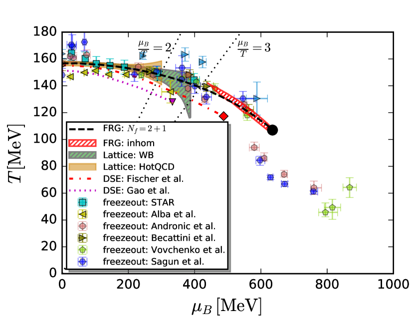
Figure 1: Phase diagram for $N_{f}=2+1$ flavour QCD in comparison to other theoretical approaches and phenomenological freeze-out data. Our result for the chiral crossover is depicted by the black dashed line. The crossover temperature has been determined through the peak position of the thermal susceptibility of the renormalised light chiral condensate, $\partial_{T}\Delta_{l,R}$, at fixed baryon chemical potential $\mu_{B}$. For more details see Section V.1, and in particular Figure 10. We show dotted black lines for $\mu_{B}/T=2,3$ to indicate the reliability bounds for the lattice and functional methods.
The phase boundary globally agrees well with recent lattice results. In particular the curvature of the phase boundary for small chemical potential, $\kappa=0.0142(2)$, is consistent with recent lattice results, $\kappa=0.0149(21)$ in Bellwied et al. (2015), $\kappa=0.0144(26)$ in Bonati et al. (2018), and $\kappa=0.015(4)$ in Bazavov et al. (2019), for an overview see D’Elia (2019). We find a critical end point at $(T_{\text{\tiny CEP}},{\mu_{B}}_{\text{\tiny CEP}})=(107,635)\,\text{MeV}$. Indications for an inhomogeneous regime close to the chiral phase transition for $\mu_{B}\gtrsim 420$  MeV are depicted by the hatched red area. For quantitative statements in this area the current approximation has to be upgraded systematically. Accordingly the hatched red area also serves as a reliability bound for the current approximation. For more details see Section V.2 and Figure 21.
Other theoretical results: lattice QCD based on an analytic continuation from the imaginary chemical potential Bellwied et al. (2015) (WB), lattice QCD based on a Taylor expansion in chemical potential Bazavov et al. (2019) (HotQCD), DSE approach with backcoupled quarks and a dressed vertex Fischer et al. (2014a) (Fischer et al.), and DSE calculations with a gluon model Gao et al. (2016) (Gao et al.).
Freeze-out data: Adamczyk et al. (2017) (STAR), Alba et al. (2014) (Alba et al.), Andronic et al. (2018) (Andronic et al.), Becattini et al. (2017) (Becattini et al.), Vovchenko et al. (2016) (Vovchenko et al.), and Sagun et al. (2018) (Sagun et al.). Note that freeze-out data from Becattini et al. with (light blue) and without (dark green) afterburner-corrections are shown in two different colors.

Our study cumulates in a prediction for the QCD phase diagram for $\mu_{B}/T\lesssim 6$. For $N_{f}=2+1$ it is presented in Figure 1 on the next page together with a survey of other theoretical predictions as well as a compilation of freeze-out points from different incarnations of the hadron resonance gas. We define the chiral phase boundary through the renormalised light chiral condensate $\Delta_{l,R}$. At small and intermediate baryon chemical potential the transition is a crossover. At $\mu_{B}=0$ the pseudocritical temperature is $T_{c}=156$ MeV. The curvature of the chiral phase boundary at small chemical potential is $\kappa=0.0142(2)$. With increasing $\mu_{B}$, the crossover becomes sharper and we find a critical endpoint at

$$(T_{\text{\tiny CEP}},{\mu_{B}}_{\text{\tiny CEP}})=(107,635)\,\text{MeV}\,.$$ (1)

Our results for the chiral phase boundary are depicted by the black dashed line in Figure 1.

In addition to a CEP, we also find indications for an inhomogeneous regime for $\mu_{B}\gtrsim 420$ MeV in the vicinity and above the chiral phase boundary. It is given by the region in the phase diagram where mesonic dispersion relation develop a minimum at nonvanishing spatial momentum, for more details we refer to Section V.2. This indicates a potential instability towards the formation of an inhomogeneous quark condensate. The region where this regime has significant overlap with the homogeneous chiral condensate is shown by the red hatched area in Figure 1. Within this area, a competition between homogeneous and inhomogeneous quark condensation has to be taken into account. Hence, this already suggests that the systematic error of the present approximation grows large for $\mu_{B}/T\gtrsim 3$.

In Figure 1 also we compare our results to recent predictions of lattice gauge theory for the phase structure at small $\mu_{B}/T$ from the Wuppertal-Budapest Collaboration Bellwied et al. (2015) (WB) and the HotQCD Collaboration Bazavov et al. (2019) (HotQCD). Our result for the pseudocritical temperature and the curvature of the phase boundary agree very well with the lattice. We also show predictions of the DSE approach from different groups, Fischer et al. (2014a) (Fischer et al.) and Gao et al. (2016) (Gao et al.). Finally we included the freeze-out data from Adamczyk et al. (2017) (STAR), Alba et al. (2014) (Alba et al.), Andronic et al. (2018) (Andronic et al.), Becattini et al. (2017) (Becattini et al.), and Vovchenko et al. (2016) (Vovchenko et al.). The freeze-out points are surprisingly close to our result for the chiral phase boundary, even at larger $\mu_{B}$. All in all, we see that a consistent picture of the QCD phase boundary at finite density starts to emerge form a culmination of results from different sources.

In order to discuss the implication for CEP searches, it is instructive to convert $\mu_{B}$ to the center-of-mass beam energy per nucleon, $\sqrt{s}$. Assuming the connection between these quantities is captured by the statistical hadronisation scenario, one finds to a very good approximation for central collisions the relation $\sqrt{s}=(a/\mu_{B}-1)/b$ with $a=1307.5\,\text{MeV}$ and $b=0.288\,\text{GeV}^{-1}$ Andronic et al. (2018). This yields for our prediction of the location of the CEP the beam energy

$$\sqrt{s_{\text{\tiny CEP}}}\approx 3.7\,\text{GeV}\,.$$ (2)

This is clearly below the smallest beam energy of current BES measurements of $\sqrt{s}=7.7\,\text{GeV}$, but well within reach of future experiments such as FAIR’s SIS100 Friman et al. (2011), NICA MPD Sorin et al. (2011), J-PARC HI Sakaguchi (2017), and STAR’s Fixed-Target (FXT) program Meehan (2016), see also Dainese et al. (2019); Alemany et al. (2019); Adamova et al. (2019). Our results therefore provide a strong motivation for CEP searches at these future experiments. Furthermore, the inhomogeneous regime appears to be also within reach of heavy-ion collisions at small beam-energies. Hence, looking for experimental signatures of this regime might be a worthwhile endeavour.

This work is organised as follows. In Section II we introduce the functional renormalisation group approach to QCD. In Section III, IV we discuss in detail the underlying systematic truncation scheme, and specify the flows for correlation functions including the propagators, vertices, and the effective potential. In Section V we present the numerical results and discuss them in detail. In Section VI we analyse the systematic error in the current approximation, also in relation to that of other functional approaches. In Section VII we close with a short summary. Many technical details of our calculations are deferred to the appendices.

II Functional renormalisation group approach to QCD

Here we discuss the functional renormalisation group approach to QCD. Our study is based on and extends the work on QCD in Braun et al. (2010a); Braun (2009); Braun et al. (2011a); Mitter et al. (2015); Braun et al. (2016a); Rennecke (2015a); Cyrol et al. (2016, 2018a, 2018b) and also draws from results on the QCD phase structure within low energy effective theories (LEFTs), Pawlowski and Rennecke (2014); Fu and Pawlowski (2015, 2016); Fu et al. (2016); Rennecke and Schaefer (2017); Braun et al. (2017); Fu et al. (2018a, b); Braun et al. (2018). For a selection of fRG studies within LEFTs see Schaefer and Wambach (2005, 2007); Herbst et al. (2011); Skokov et al. (2010, 2011); Braun et al. (2012); Strodthoff et al. (2012); Fukushima and Pawlowski (2012); Aoki and Sato (2013); Kamikado et al. (2013); Jiang and Zhuang (2012); Haas et al. (2013); Herbst et al. (2014, 2013); Tripolt et al. (2014); Grahl and Rischke (2013); Mitter and Schaefer (2014); Herbst et al. (2014); Morita et al. (2013); Pawlowski and Rennecke (2014); Helmboldt et al. (2015); Khan et al. (2015); Wang and Zhuang (2016); Mueller and Pawlowski (2015); Eser et al. (2015); Weyrich et al. (2015); Fu and Pawlowski (2015); Aoki et al. (2016); Fejos (2015); Jiang et al. (2016); Fu and Pawlowski (2016); Fu et al. (2016); Rennecke and Schaefer (2017); Jung et al. (2017); Fejos and Hosaka (2016); Almasi et al. (2017a); Posfay et al. (2018); Yokota et al. (2016); Springer et al. (2017); Resch et al. (2019); Tripolt et al. (2018a); Braun et al. (2017); Fejos and Hosaka (2017); Yokota et al. (2017); Almasi et al. (2017b); Zhang et al. (2017); Aoki et al. (2018); Braun et al. (2018); Fejos and Hosaka (2018); Braun et al. (2019a); Fu et al. (2018a, b); Sun et al. (2018); Wen et al. (2019); Yin et al. (2019); Leonhardt et al. (2019); Li et al. (2019a). For QCD-related reviews on the fRG approach see Berges et al. (2002); Pawlowski (2007); Schaefer and Wambach (2008); Gies (2012); Rosten (2012); Braun (2012); Pawlowski (2014).

II.1 QCD with dynamical hadronisation

The fRG approach is based on an infrared regularisation for momentum modes $p^{2}\lesssim k^{2}$ of the theory at hand, where $k$ is the infrared (IR) cutoff scale. This is achieved by adding a momentum-dependent mass term to the action which vanishes for momenta $p^{2}\gtrsim k^{2}$. Accordingly, the ultraviolet quantum fluctuations of the theory with momenta $p^{2}\gtrsim k^{2}$ are untouched. In turn, in the presence of the infrared cutoff, quantum fluctuations with momenta $p^{2}\lesssim k^{2}$ carry a mass proportional to $k$ and are therefore suppressed. The presence of this regulator leads to a scale dependent effective action $\Gamma_{k}$, which includes quantum fluctuations of momentum modes $p^{2}\gtrsim k^{2}$.

Thus, in the ultraviolet (UV) at large cutoff scales, $k^{2}/\Lambda_{\textrm{QCD}}^{2}\gg 1$, the effective action $\Gamma_{k}$ tends towards the bare QCD action, which is well under control with perturbation theory. This can be used as the starting point of a renormalisation group (RG) evolution of $\Gamma_{k}$, where the IR cutoff scale $k$ plays the r$\hat{\textrm{o}}$le of an RG scale. By evolving $\Gamma_{k}$ from the UV to the IR, quantum fluctuations at a given momentum scale $p^{2}\propto k^{2}$ are included successively, and the full quantum theory of QCD is resolved as $k\rightarrow 0$. $\Gamma_{k=0}$ is the full quantum effective action of QCD. Its flow $k\partial_{k}\Gamma_{k}$, is given by the Wetterich equation Wetterich (1993), see also Ellwanger (1994a); Morris (1994). It is evident from the discussion above that the fRG is a practical realisation of the Wilson RG.

At low energies or momenta the dynamical degrees of freedom of QCD are hadrons rather than quarks and gluons. The offshell dynamics relevant for the flow equation is then dominated by the lightest hadrons. At small and intermediate densities, these are the pseudo-Goldstone bosons of spontaneous chiral symmetry breaking, in particular the pseudoscalar pions $\bm{\pi}$, and the scalar resonance $f_{0}(500)$, or $\sigma$. Formulated in terms of the fundamental degrees of freedom, this requires taking care of the scalar-pseudoscalar four-quark interaction channels where these mesons emerge as resonances, as well as their scatterings. This is done conveniently by introducing a composite field

$$\phi\propto\bar{q}(T_{f}^{0},i\gamma_{5}T_{f}^{a})q\,,$$ (3)

where $q$ is a Dirac spinor with $N_{f}$ flavours and $N_{c}$ colours. $T_{f}^{a}\,,a\!=\!1,\dots,N_{f}^{2}-1$ are the generators of the $SU(N_{f})$ flavour group and $T^{0}_{f}=\mathbb{1}/\sqrt{2N_{f}}$. For example, in the two-flavour case with up and down quarks, $q=(u,d)$ we have the tensor structure $(i\gamma_{5}\bm{\sigma}/2)$, where $\bm{\sigma}=(\sigma_{1},\sigma_{2},\sigma_{3})$ are the Pauli matrices. This part of $\phi$ then corresponds to the three pions. The full field $\phi$ reflects the underlying $SU(N_{f})$ flavour symmetry for $N_{f}=2$, which translates into a $O(4)$ symmetry for $\phi$ in case of isospin symmetric matter. In the physically more relevant case of $N_{f}=2+1$ with the light $l=(u,d)$ quarks, the heavy $s$ quark and $q=(l,s)$ we simply embed (3) accordingly. This is discussed later, see (16).

The systematic introduction of the composite field $\phi$ in the fRG approach is done via dynamical hadronisation, see Refs. Gies and Wetterich (2002, 2004); Pawlowski (2007); Floerchinger and Wetterich (2009). The present formulation follows Pawlowski (2007); Braun et al. (2016a); Mitter et al. (2015); Cyrol et al. (2018a): we introduce a scale-dependent composite field $\hat{\phi}_{k}(q,\bar{q})$ and $\phi=\langle\hat{\phi}_{k}\rangle$ through a source $\int_{x}\!J_{\phi}\,\hat{\phi}_{k}$ and a respective regulator term. This field carries scalar and pseudoscalar quantum numbers. The effective action is then given by a modified Legendre transformation of the Schwinger functional $W_{k}[J]$ w.r.t. the current

$$J=(J_{A},J_{c},J_{\bar{c}},J_{q},J_{\bar{q}},J_{\phi})\,,$$ (4)

including that of the composite field $\hat{\phi}_{k}$. This leads us to

$$\Gamma_{k}[\Phi]=\int_{x}J\cdot\Phi-W_{k}[J]-\Delta S_{k}[\Phi]\,,$$ (5)

with the currents $J[\Phi]$ defined by the equations of motion (EoM),

$$J=\frac{\delta\left(\Gamma_{k}[\Phi]+\Delta S_{k}[\Phi]\right)}{\delta\Phi}\,,$$ (6)

and the cutoff term

$$\Delta S_{k}[\Phi]=\frac{1}{2}\int_{p}\Phi(-p)\cdot R_{k}(p)\cdot\Phi(p)\,.$$ (7)

The cutoff term implements the IR regularisation though a momentum dependent mass-like term, as discussed above. The components of the superfield $\Phi$ in (5), (7) are gluons, ghosts, quarks and the scalar-pseudoscalar mesonic field $\phi$,

$$\Phi=(\Phi_{f},\phi)\,,\qquad\Phi_{f}=(A,c,\bar{c},q,\bar{q})\,,\quad\phi=(\sigma,\bm{\pi})\,,$$ (8)

and $q=l$ with $l=(u,d)$ for $N_{f}=2$, and $q=(l,s)$ for $N_{f}=2+1$. Note also that the cutoff term includes an infrared regularisation with $R_{\phi}$ for the composite field. This leads us to the regulator matrix

$$R_{k}=\begin{pmatrix}R_{A}&0&0&0&0&0\\[4.30554pt] 0&0&-R_{c}&0&0&0\\[4.30554pt] 0&R_{c}&0&0&0&0\\[4.30554pt] 0&0&0&0&-R_{q}&0\\[4.30554pt] 0&0&0&R_{q}&0&0\\[4.30554pt] 0&0&0&0&0&R_{\phi}\end{pmatrix}\,.$$ (9)

The regulator $R_{k}(p)$ specifies the momentum dependence of the mass-like cutoff. It is chosen such that it suppresses quantum fluctuations with momenta smaller than the cutoff scale, $p^{2}\lesssim k^{2}$, while it leaves the UV physics with momenta $p^{2}\gtrsim k^{2}$ unaffected. Furthermore, to recover the full quantum effective action at $k=0$, we demand $R_{k\rightarrow 0}\rightarrow 0$.

This setup is closely related to a two-particle irreducible (2PI) or rather two-particle point irreducible (2PPI) formulation. If also considering the density channel $\bar{q}\gamma_{0}q$ it resembles density functional theory, for a more detailed discussion of these relations for generic composite fields see Pawlowski (2007).

The scale evolution of $\hat{\phi}_{k}$, or rather its expectation value $\langle\partial_{t}\hat{\phi}_{k}\rangle$, can be chosen freely. Its choice corresponds to a reparameterisation of the theory. We emphasise that the mean field $\phi=\langle\hat{\phi}_{k}\rangle$ in the effective action is $k$-independent. Note also that on the EoS of the auxiliary field the effective action reduces to the standard effective action of QCD in terms of the fundamental fields, $\Gamma_{\textrm{QCD}}[\Phi_{\textrm{f}}]$: The EoM of the composite field including the cutoff term entail a vanishing current,

$$J_{\phi}=\left.\frac{\delta\Gamma_{k=0}[\Phi]}{\delta\phi}\right|_{\phi_{\textrm{EoM}}[\Phi_{f}]}=0\,.$$ (10)

Since the composite field is introduced only trough the source $J_{\phi}$ and its regulator $R_{\phi}$ in the first place, the EoM (10) removes $\hat{\phi}_{k}$ from the path integral at vanishing cutoff, reducing it to the standard gauge fixed path integral of QCD. We are led to

$$\Gamma_{\textrm{QCD}}[A,c,\bar{c},q,\bar{q}]=\Gamma_{k=0}[\Phi_{f},\phi_{\textrm{EoM}}[\Phi_{f}]]\,.$$ (11)

At finite cutoff scale the composite field can also be eliminated. There, vanishing of the current $J_{\phi}$ is obtained for $\delta(\Gamma_{k}+\Delta S_{k})/\delta\phi=0$, and the infrared regularised path integral at $J_{\phi}=0$ still depends on the cutoff term of the composite field. This amounts to inserting a UV-irrelevant four-quark interaction in the classical QCD action. This procedure does not spoil the renormalisability as a pointlike NJL-type interaction does, but solely provides an IR regularisation of the respective resonant four-quark interaction.

In summary this setup encodes the full information of the QCD correlation functions but also allows for a simple access to bound state information such as the Bethe-Salpeter wave functions, see Mitter et al. (2015); Braun et al. (2016a); Cyrol et al. (2018b); Alkofer et al. (2019). Note also that in general the QCD correlation functions now involve derivatives of the composite field. As an important example we consider general four-quark vertices. They are given by functional derivatives of the QCD effective action $\Gamma_{\textrm{QCD}}$ on the EoM $\Phi_{f,\textrm{EoM}}=0$ at $T$. At finite temperature $\Phi_{f,\textrm{EoM}}$ contains a nonvanishing temporal gluon background field, $A_{0,\textrm{EoM}}$, which carries the information of confinement, see Braun et al. (2010a, b); Fister and Pawlowski (2013); Herbst et al. (2015).

If the composite field $\phi$ is simply proportional to a quark bilinear as indicated in (3), the four-quark derivatives of (11) lead us to

$$\Gamma^{(4)}_{\textrm{QCD},q_{1}\bar{q}_{1}q_{2}\bar{q}_{2}}[0]=\Gamma^{(4)}_{0,q_{1}\bar{q}_{1}q_{2}\bar{q}_{2}}[0,\phi]$$

$$+\int_{x}\frac{\delta^{2}\phi(x)}{\delta q_{1}\delta\bar{q}_{1}}\Gamma^{(3)}_{0,q_{2}\bar{q}_{2}\phi}[0,\phi]+\textrm{permut.}$$

$$+\int_{x,y}\frac{\delta^{2}\phi(x)}{\delta q_{1}\delta\bar{q}_{1}}\frac{\delta^{2}\phi(y)}{\delta q_{2}\delta\bar{q}_{2}}\Gamma^{(2)}_{0,\phi\phi}[0,\phi]+\textrm{permut.}\,.$$ (12)

In (12) it is understood that $\phi=\phi_{\textrm{EoM}}[\Phi_{f}]$, and we have restricted ourselves to the $T=0$ case with $\Phi_{f,\textrm{EoM}}=0$. In (12) we have also introduced our notation for $n$-point correlation functions or vertices,

$$\qquad\Gamma^{(n)}_{\Phi_{i_{1}}\cdots\Phi_{i_{n}}}[\Phi]=\frac{\delta^{n}\Gamma[\Phi]}{\delta\Phi_{i_{1}}\cdots\delta\Phi_{i_{n}}}\,.$$ (13)

If we choose the composite field such that it completely absorbs a given momentum channel in the four-quark scattering, the first term on the right hand side in (12) vanishes and we are left with exchange terms of the composite field. For example, for the pseudoscalar channel the second and third line in (12) comprise terms with a pion propagator $(1/\Gamma^{(2)})_{\pi\pi}$ with two Bethe-Salpeter wave functions $\Gamma^{(3)}_{q\bar{q}\pi}$ attached.

Note also that nontrivial terms such as in the second and third line of (12) only occur in correlation functions of the fundamental fields $\Phi_{f}$ for more than one quark-antiquark pair. For example, for the quark two-point function or inverse propagator we find schematically

$$\Gamma^{(2)}_{\textrm{QCD},q_{1}\bar{q}_{1}}=\Gamma^{(2)}_{0,q_{1}\bar{q}_{1}}+\int\frac{\delta^{2}\phi}{\delta q_{1}\delta\bar{q}_{1}}\Gamma^{(1)}_{0,\phi}=\Gamma^{(2)}_{0,q_{1}\bar{q}_{1}}\,,$$ (14)

with $\phi=\phi_{\textrm{EoM}}[\Phi_{f}]$. Then the term proportional to $\Gamma^{(1)}_{0,\phi}$ vanishes as the latter is the EoM for $\phi$. Finally we use $\Phi_{f}=0$ as in (12).

For the dynamical hadronisation in the present work we use the option of absorbing the dominant four-quark interaction channel completely. This is achieved by choosing the flow of $\hat{\phi}_{k}$ such that the scalar-pseudoscalar channel in the effective four-quark interaction of the light quarks $u,d$ is eliminated. Formally, this can be viewed as a successive bosonisation in terms of a Hubbard-Stratonovich transformation of this interaction channel at each RG scale $k$. For more details see Section III.5. This puts forwards the general hadronisation relation

$$\langle\partial_{t}\hat{\phi}_{k}\rangle= \dot{A}_{k}\,\bar{q}\tau q+\dot{B}_{k}\,\phi+\dot{C}_{k}\,\hat{e}_{\sigma}\,,$$ (15)

with $\tau=(T_{2}^{0},i\gamma_{5}\bm{T}_{2})$ and $T_{f}^{a}$ defined in (3). The vector $\hat{e}_{\sigma}$ points in the $\sigma$-direction, with the convenient normalisation $\hat{e}_{\sigma}=1/\sqrt{2N_{f}}$ matching that of $\tau$. Since we only consider the dynamical hadronisation of the $\bm{\pi}$–$\sigma$ channel of the light quarks, we embed the $SU(2)$ scalar-pseudoscalar field $(\sigma,\bm{\pi})$ into $SU(3)$. This implies in (15),

$$\tau^{a}_{N_{f}=2+1}=\begin{pmatrix}\tau^{a}&0\\[4.30554pt] 0&0\end{pmatrix}\,,$$ (16)

in a slight abuse of notation. The hadronisation functions $\dot{A}_{k}$, $\dot{B}_{k}$ and $\dot{C}_{k}$ can be chosen freely. The hadronisation function $\dot{A}_{k}$ controls the overlap of $\phi$ with the scalar-pseudoscalar channel, while $\dot{B}_{k}$ simply changes the wave function renormalisation $Z_{\phi}$ of the composite field. The latter function can e.g. be used to conveniently choose $Z_{\phi}=1$. As it does not change the parameterisation of the theory we discard it in the following, using $\dot{B}_{k}=0$.

Finally, the hadronisation function $\dot{C}_{k}$ introduces a shift in the scalar field $\sigma$. In general, this shift can be used to entirely absorb the quark mass of the respective quark flavour, leading to chiral quarks. However, this comes at the expense of diffusing the symmetry properties of the effective action. For example, if we start with a $\mathbf{Z}_{2}$-symmetric effective potential $V(\sigma)=V(-\sigma)$ necessary (but not sufficient) for chiral symmetry, a shift in $\sigma$ introduces odd powers in the $\sigma$ field in the effective potential. Of course, chiral symmetry is not lost, but the respective symmetry transformation is not simply $\sigma\to-\sigma$ anymore. A prominent example is the $\sigma$-mass term $1/2m_{\sigma}^{2}\sigma^{2}$. A shift in $\sigma$ with $\sigma\to\sigma-c_{\sigma}/m_{\sigma}^{2}$ leads to a linear term in the effective action,

$$\Gamma_{k}[\Phi]\propto-\int_{x}c_{\sigma}\,\sigma\,,$$ (17)

while still keeping the original $\sigma$-mass term. In the presence of higher powers of $\sigma$, more $\sigma$-odd terms are generated as well as changing the coefficients of the $\sigma$-even terms. Consequently we expect that $\dot{C}_{k}$ cannot be chosen freely if we restrict ourselves to dynamical hadronisation setups that keep chiral symmetry apparent. Indeed this constraint leads us to $\dot{C}_{k}\equiv 0$, see Appendix B.

The linear term (17) plays a special r$\hat{\textrm{o}}$le in the effective action. To see this more clearly, we solve the Legendre transform (5) for the Schwinger functional and use the EoM for the current leading to $J[\Phi]$ defined in (6). With these definitions (17) implies that $J[\Phi]$ contains the term $-c_{\sigma}$. Then, the Schwinger functional reads,

$$W_{k}[J]=\int_{x}J\cdot\Phi-\Gamma_{k}[\Phi]-\Delta S_{k}[\Phi]\,,$$ (18)

where $J=J[\Phi]$. Evidently the $c_{\sigma}$-dependences in the first two terms on the right hand side of (18) cancel each other. We conclude already from here that the flow equation of the effective action with dynamical hadronisation should be explicitly $c_{\sigma}$-independent. Moreover, necessarily the left hand side of (18) is also $c_{\sigma}$-independent. Consequently, the $c_{\sigma}$-dependence of the current in the Schwinger functional is canceled by that of $W_{k}[0]$. This leaves us with

$$W_{k}[J]=\widehat{W}_{k}[\hat{J}]\quad\textrm{with}\quad\widehat{W}_{k}=\left.W_{k}\right|_{c_{\sigma}=0}\,,$$ (19)

and $J=J[\Phi]$ satisfies the EoM (6). The current is shifted in the $J_{\sigma}$-direction, $\hat{J}[\Phi]=J[\phi]+c_{\sigma}\delta_{\Phi\sigma}$, in components:

$$\hat{J}=(J_{A},J_{c},J_{\bar{c}},J_{q},J_{\bar{q}},J_{\sigma}+c_{\sigma},J_{\pi})\,.$$ (20)

The shifted current $\hat{J}[\Phi]$ in (20) does not depend on $c_{\sigma}$, that is $\partial_{c_{\sigma}}\hat{J}\equiv 0$. With these relation we finally arrive at a convenient form of the effective action,

$$\Gamma_{k}[\Phi]=\int_{x}J\cdot\Phi-\widehat{W}_{k}[\hat{J}]-\Delta S_{k}[\Phi]\,,$$ (21)

We would like to elucidate the above relations within a simple example which is relevant in the present context: Consider a composite $\sigma$-field that is just proportional to the scalar quark bilinear,

$$\hat{\sigma}_{k}=-D_{k}\,\hat{\bar{q}}\hat{q}\,,$$ (22)

with a cutoff dependent prefactor $D_{k}$. Note that the hats indicate that this relation holds on the level of the fluctuation fields in the path integral. We also emphasise that our example (22) has an overlap with the first term in the dynamical hadronisation flow (15) with $\dot{A}_{k}=-\partial_{t}D_{k}$, but is not identical: $\langle\hat{\bar{q}}\hat{q}\rangle=\bar{q}q+G_{\bar{q}q}[\Phi]$. Importantly, the linear term $-\int_{x}c_{\sigma}\sigma$ in the effective action (17) is in one to one correspondence to the quark (current) mass term in the classical action, $S_{\textrm{QCD}}\propto m^{0}_{q}\int\hat{\bar{q}}\hat{q}$. Obviously, the latter term can be absorbed into a shift of the source term for $\hat{\sigma}$ with

$$-m^{0}_{q}\int\hat{\bar{q}}\hat{q}+\int_{x}J_{\sigma}\hat{\sigma}_{k}=\int_{x}\hat{J}_{\sigma}\hat{\sigma}_{k}\,,$$ (23)

where

$$\hat{J}_{\sigma}=J_{\sigma}+c_{\sigma}\,,\quad\textrm{with}\quad c_{\sigma}=\frac{m^{0}_{q}}{D_{k}}\,.$$ (24)

We conclude that the Schwinger functional with a source for the composite field $\hat{\sigma}_{k}$ in (22) and the classical QCD action with a quark current mass term, $S_{\textrm{QCD}}\propto m^{0}_{q}\int\hat{\bar{q}}\hat{q}$, is that in the chiral limit with $m^{0}_{q}=0$ and a shifted current for the composite field. However, $m^{0}_{q}=0$ simply is $c_{\sigma}=0$, see (24), and we arrive at

$$W_{k}[J_{\sigma}]=\left.W_{k}[\hat{J}_{\sigma}]\right|_{m_{q}=0}=\widehat{W}_{k}[\hat{J}_{\sigma}]\,.$$ (25)

Note that (25) entails that the full dynamics of QCD in the presence of explicit chiral symmetry breaking is that of the theory with a composite condensate field $\hat{\sigma}$ with full chiral symmetry: The explicit chiral symmetry breaking is completely absorbed in a shift of the external current $J\to\hat{J}$.

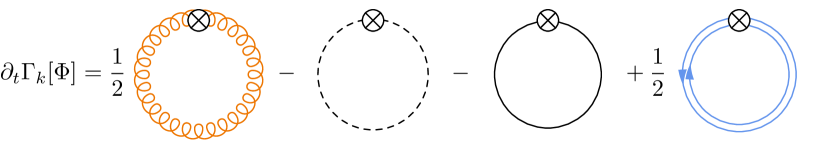
Figure 2: Flow of the effective action of QCD. The first three diagrams arise from the gluon, ghost, and the quark degrees of freedom respectively. The last diagram is that of the mesonic contribution. The double line with the up-down arrows indicates the nature of the mesons as quark-antiquark composites. The crossed circles indicate the regulator insertion in the flow equation.

In summary this leads us to the flow equation for QCD with dynamical hadronisation, Pawlowski (2007); Rennecke (2015b),

$$\begin{split}&\partial_{t}\Gamma_{k}[\Phi]+\int\langle\partial_{t}\hat{\phi}_{k,i}\rangle\,\left(\frac{\delta\Gamma_{k}[\Phi]}{\delta\phi_{i}}+c_{\sigma}\delta_{i\,\sigma}\right)\\[4.30554pt] &\quad=\frac{1}{2}\operatorname{Tr}\!\big{(}G_{k}[\Phi]\,\partial_{t}R_{k}\big{)}+\frac{1}{2}\operatorname{Tr}\!\bigg{(}G_{\phi\Phi_{j}}[\Phi]\frac{\delta\langle\partial_{t}\hat{\phi}_{k}\rangle}{\delta\Phi_{j}}\,R_{\phi}\bigg{)}\,,\end{split}$$ (26)

with the RG time $t=\ln(k/\Lambda)$, and

$$G_{k}[\Phi]=\frac{1}{\Gamma^{(2)}_{k}[\Phi]+R_{k}}\,,\qquad G_{\Phi_{i}\Phi_{j}}[\Phi]=\left(G_{k}[\Phi]\right)_{\Phi_{i}\Phi_{j}}\,.$$ (27)

The shift in the dynamical hadronisation term in the first line in (26) subtracts the explicit chiral symmetry breaking term in $\Gamma^{(1)}_{\sigma}$. The $t$-derivative $\partial_{t}\Gamma_{k}$ in (26) is taken at fixed $c_{\sigma}$ as the $\dot{c}_{\sigma}$ terms from $\partial_{t}\Gamma_{k}$ cancel with that from $\partial_{t}\int J\cdot\Phi\propto\partial_{t}\int(\partial_{t}J_{\textrm{sym}})\cdot\Phi-\int\dot{c}_{\sigma}\sigma$. The $(\partial_{t}J_{\textrm{sym}})$-terms are cancel by those from the Schwinger functional in (21). We emphasise that (26) is explicitly $c_{\sigma}$-independent, and is a novel representation of dynamical hadronisation.

Note also that (26) with (15) entails that we do not have to specify $\hat{\phi}_{k}$ but only the expectation value of its flow, $\langle\partial_{t}\hat{\phi}_{k}\rangle$, as done in (15). The second term in the first line of (26) accounts for the cutoff dependence of the reparameterisation that originates in the cutoff dependence of $\hat{\phi}_{k}$. It can be understood as a generalised anomalous dimension of $\phi$. Indeed, for

$$\langle\partial_{t}\hat{\phi}\rangle=-\frac{1}{2}\eta_{\phi}\phi\,,$$ (28)

this term carries nothing but the anomalous rescaling of the composite field $\phi$. However, we emphasise again that $\partial_{t}$ is a derivative at fixed mean superfield $\Phi$, and in particular at fixed $\phi$. The second term in the second line also accounts for the cutoff dependence of the reparameterisation via $\partial_{t}\hat{\phi}_{k}$.

The first term in the second line of (26) is the standard functional flow. The trace sums over momenta, internal indices and species of fields including the composite field. More explicitly it reads

$$\begin{split}\frac{1}{2}\operatorname{Tr}G_{k}\,\partial_{t}R_{k}=&\,\frac{1}{2}\operatorname{Tr}G_{AA}\,\partial_{t}R_{A}-\operatorname{Tr}\,G_{c\bar{c}}\,\partial_{t}R_{c}\\[4.30554pt] &-\operatorname{Tr}G_{q\bar{q}}\,\partial_{t}R_{q}+\frac{1}{2}\operatorname{Tr}G_{\phi\phi}\,\partial_{t}R_{\phi}\,,\end{split}$$ (29)

where all propagators are $\Phi$-dependent. We show the flow equation (26) with $\partial_{t}\hat{\phi}=0$ diagrammatically in Figure 2 for QCD. The first gluon and ghost diagrams constitute the glue contributions, and the last two arise from the matter sector, which are the quark and meson degrees of freedom, respectively. Note that the scalar and pseudoscalar mesonic loops are present here because we introduced them explicitly with dynamical hadronisation. This is nothing but a convenient parametrisation of resonant interaction channels. We emphasise that the absense of explicit loops for other hadrons, e.g. other mesons and baryons, does not entail that their dynamics is not included.

III Truncation scheme

In this section we discuss in detail the expansion scheme for the effective action and the flow equations used in the present work. This includes in particular a discussion of the approximations used, and their quantitative or qualitative validity.

III.1 Vertex expansion

In QCD, (26) can only be solved within given truncations to the effective action. The systematic expansion scheme behind such approximations is the vertex expansion. It is an expansion of the effective action in powers of the field, the expansion coefficients being the $n$-point functions $\Gamma^{(n)}(p_{1},...,p_{n})$. Typically, this expansion shows a rather good convergence if no divergent exchange processes or couplings are present. In Landau gauge QCD the strong couplings related to gluon exchange grow towards the infrared but tend to zero for momenta or cutoff scales below approximately one GeV, reflecting the QCD mass gap, see Mitter et al. (2015); Braun et al. (2016a); Rennecke (2015a, b); Cyrol et al. (2018a). This behaviour supports the apparent convergence of the vertex expansion. Another source for divergent exchange processes are resonant interactions that potentially spoil or at least slow down the convergence of the vertex expansion. In particular for this reason dynamical hadronisation is crucial as it controls the resonant interaction channels and allows to take into account multi-scatterings of resonances in a technically accessible way via the respective effective potential of the composite fields.

III.2 Expansion about vacuum QCD & finite temperature Yang-Mills theory

We can rely on quantitative results for vacuum Yang-Mills theory, Cyrol et al. (2016) and $N_{f}=2$ flavour QCD, Mitter et al. (2015); Cyrol et al. (2018a), and finite temperature Yang-Mills theory, Cyrol et al. (2018b), as input as well as benchmark tests for our current computations. State-of-the-art truncations which involve a large set of correlation functions have been used in these works.

Furthermore, it is well-known that mild momentum-dependences of vertex functions and propagators are well captured by scale-dependent dressing functions; for investigations in QCD and low energy effective models see e.g. Helmboldt et al. (2015); Pawlowski and Rennecke (2014); Braun et al. (2016a); Rennecke (2015b); Rennecke and Schaefer (2017). This suggests an approximation scheme in which only the dominant nontrivial momentum dependences are taken into account explicitly, while the rest of the dependences is approximated by scale-dependent dressings.

This approach has been successfully applied to vacuum QCD in Braun et al. (2016a); Rennecke (2015a, b) and for QCD at finite temperature and imaginary chemical potential in Braun et al. (2011a). In these works QCD flows have been expanded about the full gluon and ghost two-point functions of Yang-Mills theory. All other correlation functions considered there have been approximated with scale-dependent dressings. Schematically we decompose the two-point functions as $\Gamma^{(2)}\simeq Z\,S^{(2)}_{\textrm{kin}}+$ (additional tensor structures). For example, for the quark, $S^{(2)}_{\textrm{kin}}$ carries the Dirac term, while the mass term is buried in the additional tensor structures. For the gluon this entails for the two-point function is $\Gamma^{(2)}_{AA}(p)\simeq Z_{A}(p^{2})\,S^{(2)}_{AA}(p)$, but we have to consider different Lorentz tensors. The nontrivial momentum- and scale-dependence of the kinetic term of a given field is fully captured by the anomalous dimensions,

$$\eta_{\Phi_{i}}=-\frac{\partial_{t}Z_{\Phi_{i}}}{Z_{\Phi_{i}}}\,.$$ (30)

Note that (30) only schematically provides the anomalous dimension, we have neither specified the projection procedure nor the momentum evaluation. We further exemplify the setup with the relevant case of the gluon two-point function. There, one also utilises the observation that the anomalous dimension $\eta_{A}$ of the gluon can be parameterised in terms of the running coupling $\alpha^{\textrm{YM}}_{k}$ in Yang-Mills theory,

$$\eta_{A,k}^{\textrm{YM}}=\eta_{A}^{\textrm{glue}}\left(\alpha^{\textrm{YM}}_{k},(\bar{m}^{\textrm{YM}}_{A,k})^{2}\right)\,,$$ (31)

with the Yang-Mills running coupling $\alpha^{\textrm{YM}}_{k}$ and the transversal gluon mass parameter,

$$m_{A,k}^{2}=\left.\frac{1}{3(N_{c}^{2}-1)}\frac{1}{k^{2}}\Pi_{\mu\nu}^{\perp}(p){\Gamma^{(2)}_{AA}}^{aa}_{\mu\nu}(p)\right|_{p=0}\,,$$ (32)

where $\Pi_{\mu\nu}^{\perp}$ is the transversal projection operator, see (226). The renormalised gluon mass parameter $\bar{m}_{A}^{2}$ differs from $m_{A}^{2}$ in (32) by an appropriate renormalisation. This renormalisation has to be applied to all coupling parameters and fields and is discussed in detail in the next Section III.3. In (31) the Yang-Mills gluon mass parameter $(\bar{m}^{\textrm{YM}}_{A,k})^{2}$ has been used. $\eta_{A}^{\textrm{glue}}$ stands for all diagrams involving gluons and ghosts that contribute to the gluon anomalous dimension. This parameterisation of the glue part of the anomalous dimension allows for a simple representation of the anomalous dimension of full QCD,

$$\eta_{A,k}=\eta_{A}^{\textrm{glue}}(\alpha_{k},\bar{m}_{A,k}^{2})+\eta^{\textrm{quark}}_{A,k}\,,$$ (33)

with the full QCD coupling $\alpha_{k}$ and renormalised mass parameter $\bar{m}_{A,k}^{2}=m_{A,k}^{2}/Z_{A}$, respectively. Importantly, this setup also takes care of the backreaction of the quark fluctuations to the pure glue and ghost diagrams, for a detailed description see Braun et al. (2016a); Rennecke (2015b). A benchmark test concerns the full gluon propagator in unquenched two-flavour QCD, which has been shown to be in quantitative agreement with the lattice results in Rennecke (2015b), more details can be found in Appendix D.

A simpler approximation is given by the ‘direct sum’

$$\eta_{A,k}\approx\eta_{A,k}^{\textrm{YM}}+\eta^{\textrm{quark}}_{A,k}\,.$$ (34)

With (34) the backreaction of the quark loop on the pure glue couplings and propagators in $\eta_{A}^{\textrm{glue}}$ is neglected. While such an approximation also lacks full RG invariance, it works well for initial scales of $\Lambda\approx 10-20$  GeV. Alternatively a readjustment of the scales can be done on top of the simple approximation (34). A respective benchmark test for the full gluon propagator in unquenched two-flavour QCD has been done in Rennecke (2015b), for more details see Appendix D. The direct-sum approximation has been used very successfully in many functional applications to the phase structure of QCD, notably in fRG application to QCD, Braun et al. (2011a), as well as the DSE applications Fischer et al. (2011); Fischer and Luecker (2013); Fischer et al. (2014b, a, 2015); Eichmann et al. (2016a); Mitter et al. (2018); Fischer (2019); Isserstedt et al. (2019); Gunkel et al. (2019). We also emphasise that the approximation may get even better for large chemical potential, as the latter lifts the fermi sea and successively more quark fluctuations are buried in it. This effect reduces the impact of the quark loop on the purely gluonic correlation functions. However, this reasoning does not apply straightforwardly to the quark-gluon vertex, and has to be taken with a grain of salt beyond the onset of baryon density. Still, in summary the approximation is well-founded and well-tested.

Here we apply this promising approximation scheme to the unquenched QCD gluon propagator at vanishing temperature as well as the glue contribution at finite temperature. Let us describe this procedure with an expansion of the finite temperature and density theory about the vacuum. Schematically this is described by the following separation of the flow for a given correlation function at finite $T$ and $\mu$,

$$\partial_{t}\Gamma^{(n)}_{T,\mu}(p)=\partial_{t}\Gamma^{(n)}_{0,0}(p)+\partial_{t}\Delta\Gamma^{(n)}_{T,\mu}(p)\,,$$ (35)

where we suppressed the subscript $k$, and $\Delta\Gamma^{(n)}$ is defined by,

$$\Delta\Gamma^{(n)}_{T,\mu}(p)=\Gamma^{(n)}_{T,\mu}(p)-\Gamma^{(n)}_{0,0}(p)\,.$$ (36)

Its flow is given by the difference of the flow diagrams for the correlation function at finite $T,\mu$ and the vacuum,

$$\partial_{t}\Delta\Gamma^{(n)}_{T,\mu}(p)=\textrm{Flow}^{(n)}_{T,\mu}(p)-\textrm{Flow}^{(n)}_{0,0}(p)\,,$$ (37)

with

$$\textrm{Flow}^{(n)}_{\Phi_{i_{1}}\cdots\Phi_{i_{n}}}=\frac{\delta^{n}}{\delta\Phi_{i_{1}}\cdots\Phi_{i_{n}}}\left[\frac{1}{2}\operatorname{Tr}\,G_{k}[\Phi]\,\partial_{t}R_{k}\right]\,.$$ (38)

While the first term on the right hand side of (37) depends on $\Delta\Gamma^{(n)}_{T,\mu}(p)$ and $\Gamma^{(n)}_{0,0}(p)$, the second term is a function of only the latter vacuum correlation functions. Accordingly, the flows (37) are closed equations for the set $\{\Delta\Gamma^{(n)}\}$ of thermal and density corrections of general correlation functions $\Gamma^{(n)}_{T,\mu}$ with the given input of the set of vacuum correlation functions $\{\Gamma^{(n)}_{0,0}\}$.

In summary this allows for the use of scale-dependent dressings for $\Delta\Gamma^{(n)}$ with a mild momentum dependence at finite temperature and density, while still maintaining the quantitative nature of the approximation: Quantitative results for vacuum QCD and finite temperature Yang-Mills theory Mitter et al. (2015); Cyrol et al. (2016, 2018a, 2018b) are used for the nontrivial momentum dependences of this part of the correlation functions. Note that this setup also allows for the use of quantitative results from other approaches such as lattice simulations and DSE computations.

In the present work we apply this approach to the gluon two-point function $\Gamma^{(2)}_{AA}$. Its density corrections and thermal quark fluctuations are computed with the input of the quantitatively reliable vacuum QCD results from Cyrol et al. (2018a) and the finite temperature Yang-Mills results in Cyrol et al. (2018b). For the ghost two-point function $\Gamma^{(2)}_{c\bar{c}}$ we only use input from vacuum QCD from Cyrol et al. (2018a). The details can be found in Section IV.1.2.

III.3 Truncation for the effective action

Having captured the nontrivial momentum-dependence of the gluon propagation, we adopt the following truncation for the Euclidean scale-dependent effective action $\Gamma_{k}$ for both, $N_{f}=2$ and $N_{f}=2+1$ flavours,

$$\Gamma_{k}= \int_{x}\bigg{\{}\frac{1}{4}F^{a}_{\mu\nu}F^{a}_{\mu\nu}+Z_{c}\,(\partial_{\mu}\bar{c}^{a})D_{\mu}^{ab}c^{b}+\frac{1}{2\xi}(\partial_{\mu}A^{a}_{\mu})^{2}$$

$$+\frac{1}{2}\int_{p}A^{a}_{\mu}(-p)\left(\Gamma^{(2)}_{AA}{}^{ab}_{\mu\nu}(p)-Z_{A}\Pi_{\mu\nu}^{\perp}\delta^{ab}p^{2}\right)A^{b}_{\nu}(p)$$

$$+\bar{q}\,\bigl{[}Z_{q}\,(\gamma_{\mu}D_{\mu}-\gamma_{0}\hat{\mu})+m_{s}(\sigma_{s})\bigr{]}\,q\,$$

$$-{\lambda_{q}}\,\Big{[}(\bar{q}\,\tau^{0}q)^{2}+(\bar{q}\,\bm{\tau}q)^{2}\Big{]}+h\,\bar{q}\,\left(\tau^{0}\sigma+\bm{\tau}\cdot\bm{\pi}\right)\,q$$

$$+\frac{1}{2}Z_{\phi}\,(\partial_{\mu}\phi)^{2}+V_{k}(\rho,A_{0})-c_{\sigma}\,\sigma-\frac{1}{\sqrt{2}}\,c_{\sigma_{s}}\,\sigma_{s}\bigg{\}}\,,$$ (39)

with $\int_{x}=\int_{0}^{1/T}dx_{0}\int d^{3}x$ and $\tau=1/2(\mathbb{1},i\gamma_{5}\bm{\sigma})$ being defined in (3). Note that all couplings depend on the RG scale $k$, which in most cases is omitted for the sake of clarity. The effective potential

$$V_{k}(\rho,A_{0})=V_{\textrm{glue},k}(A_{0})+V_{\textrm{mat},k}(\rho,A_{0})\,,$$ (40)

carries a dependence on the mesonic field $\rho=(\sigma^{2}+\vec{\pi}^{2})/2$, and the temporal gauge field $A_{0}$, which is related to the Polyakov loop $L[A_{0}]$. The expectation values of these fields are approximate order parameters for the chiral phase transition ($\rho)$ and the confinement-deconfinement phase transition ($A_{0}$ or $L[A_{0}]$), for more details see Section III.6. In (40) we separated the contribution from the gluonic loop in (26), see Figure 2, that is $V_{\textrm{glue},k}$ and that of the quark and meson loops, $V_{\textrm{mat},k}$. We also neglected the subleading $\rho$-dependences of the gluon loop, $V_{\textrm{glue},k}(A_{0},\rho)\to V_{\textrm{glue},k}(A_{0})$.

The gluon two-point function $\Gamma^{(2)}_{AA}$ has been already discussed in the previous Section III.2. The subtraction with $Z_{A}p^{2}$ in the second line removes the $A^{2}$-contribution coming from the $F_{\mu\nu}^{2}$-term for avoiding double counting. In the present fRG approach the theory is fully determined by the strong running coupling $\alpha_{s,\Lambda}$ at the initial cutoff scale $k=\Lambda$ in the UV, the light current quark mass $m_{l}^{0}$ for $N_{f}=2$ and additionally the strange current quark $m_{s}^{0}$ for $N_{f}=2+1$ with the choice

$$Z_{\Phi,k=\Lambda}=1\,.$$ (41)

With dynamical hadronisation the current quark masses are encoded in $c_{\sigma}$ and $c_{\sigma_{s}}$. Their values in the physical case are fixed by the pion mass and the kaon mass. Alternatively, the pion and kaon decay constants can be used to pin down these parameters. This is explained below. The values for an initial cutoff $\Lambda=20\,$GeV can be found in Table 1 at the end of this Section.

The field strength tensor $F^{a}_{\mu\nu}$ and the covariant derivatives in the ghost and quark kinetic terms also carry a cutoff dependence, and are defined and discussed in detail in Section III.4, (60) and (57) respectively. The $Z_{\Phi_{i}}$’s are the cutoff dependent wave function renormalisations of the respective component fields $\Phi_{i}$ of the superfield defined in (8). Note that the effective action is renormalisation group invariant (but $k$-dependent) w.r.t. the underlying renormalisation group scale $\mu$ of the theory at $k=0$, for more details see Pawlowski (2007). This suggests the introduction of renormalised fields

$$\bar{\Phi}=Z_{\Phi}^{1/2}\Phi\,,$$ (42)

as well as renormalised coupling parameters, for example

$$\bar{m}_{\Phi}=\frac{m_{\Phi}}{Z^{1/2}_{\Phi}}\,,\quad\quad\bar{h}=\frac{h}{Z_{\phi}^{1/2}Z_{q}}\,.$$ (43)

Since we perform our computations in Euclidean spacetime, the renormalised masses in (43) are curvature masses in contradistinction to the physical pole masses $m_{\Phi,\textrm{pol}}$. Within the fRG setup this difference has been discussed in detail in Helmboldt et al. (2015). For example, the constituent quark masses are curvature masses. In turn, the pion pole mass $m_{\pi,\textrm{pol}}$ is used for fixing the value of explicit chiral symmetry breaking, see Table 1. For more details on the definition of the mesonic pole masses see Section IV.1.1.

Similar relations hold for the other coupling parameters and are discussed later. Note that the epithet renormalised is related to the $k$-dependence. Note also that the renormalised fields carry classical dispersions if we use fully momentum-dependent $Z_{\Phi}$’s in (42). Accordingly in pole renormalisation schemes the respective masses are pole masses. Moreover, observables are provided in terms of the renormalised fields and couplings, and we shall discuss physics in terms of these objects.

The quark chemical potential matrix $\hat{\mu}$ considered here is understood to couple to all flavours equally, $\hat{\mu}=\textrm{diag}(\mu_{q},\mu_{q},\mu_{q})$. Thus, it is directly related to the baryon chemical potential $\mu_{B}=3\mu_{q}$. The constituent quark mass $\bar{m}_{s}$ also has to be read as a diagonal flavour matrix $\textrm{diag}(0,0,\bar{m}_{s})$.

In the present work we do not consider dynamical hadronisation of the full $N_{f}=3$ flavour multiplet $T^{a}_{N_{f}}(\sigma_{a}+i\,\gamma_{5}\pi_{a})$, with the $U(N_{f})$ generators $T^{a}_{N_{f}}$, $a=0,...,N_{f}^{2}-1$. In the singlet-octet basis they are given by $T^{0}_{N_{f}}=\mathbb{1}_{N_{f}\times N_{f}}/\sqrt{2N_{f}}$ and the $SU(N_{f})$ generators $T^{i}_{N_{f}}$ for $i=1,...,N_{f}^{2}-1$. Instead, we only consider part of the embedded $N_{f}=2$ multiplet: the scalar $\sigma$ as well as the pseudoscalar pions. The four-quark interaction that gives rise to the corresponding resonances is given by $\lambda_{q}$. The other mesons of the scalar and pseudoscalar nonets are too heavy for playing a significant r$\hat{\textrm{o}}$le in the offshell dynamics. Of the strange part of the multiplet we only consider the scalar $\sigma_{s}$. The two scalars $\sigma,\sigma_{s}$ are related to the ones in the singlet-octet basis via

$$\begin{pmatrix}\sigma\\ \sigma_{s}\end{pmatrix}=\frac{1}{\sqrt{3}}\begin{pmatrix}\sqrt{2}&1\\ 1&-\sqrt{2}\end{pmatrix}\begin{pmatrix}\sigma_{0}\\ \sigma_{8}\end{pmatrix}\,,$$ (44)

for more details see e.g. Schaefer and Wagner (2009); Herbst et al. (2014); Mitter and Schaefer (2014); Rennecke and Schaefer (2017); Fu et al. (2018a); Wen et al. (2019). Both, light and strange quark constituent masses are given in terms of condensates,

$$\bar{m}_{l}=\frac{1}{2}\bar{h}\,\bar{\sigma}\,,\qquad\qquad\bar{m}_{s}=\frac{1}{\sqrt{2}}\bar{h}\,\bar{\sigma}_{s}\,,$$ (45)

with the renormalised Yukawa coupling and the renormalised $\sigma,\sigma_{s}$-expectation value $\bar{\sigma}=Z_{\phi}^{1/2}\sigma$ and $\bar{\sigma}_{s}=Z_{\phi}^{1/2}\sigma_{s}$ respectively, see (42) and (43). Their values are determined via the explicit breaking terms $c_{\sigma}\,\sigma$ and $1/\sqrt{2}\,c_{\sigma_{s}}\,\sigma_{s}$, as well as dynamical chiral symmetry breaking. Both phenomena lead to nonvanishing $\sigma_{\textrm{EoM}}$ and $\sigma_{s,\textrm{EoM}}$ and hence to nonvanishing renormalised expectation values $(\bar{\sigma},\bar{\sigma}_{s})_{\textrm{EoM}}$. The explicit breaking coefficient $c_{\sigma}$ in the light sector is fixed with the physical pion mass. Alternatively one could use the ratio of the pion decay constant $f_{\pi}$ with that in the chiral limit, $f_{\pi,\chi}$ for fixing $c_{\sigma}$, that is $f_{\pi}/f_{\pi,\chi}\approx 93/88$, Tanabashi et al. (2018). Here, we choose the pion mass instead of this ratio as it is more easily accessible. Furthermore, small errors in the determination of the pion mass only propagate to small errors in other observables. In turn, the explicit breaking coefficient $c_{\sigma_{s}}$ may be either determined by e.g. the kaon mass or the ratio $f_{K}/f_{\pi}\approx 111/93$, Tanabashi et al. (2018). We refer to Appendix E.3 for a more detailed discussion of the scale setting.

The relative size of the explicit breaking coefficients, $c_{\sigma_{s}}/c_{\sigma}$ may also be determined by their relation to the current quark masses $m_{l}^{0}$ and $m_{s}^{0}$. For large momentum scales of the order of the electro-weak scale $\sim 90$ GeV, that is in the absence of any chiral dynamics, the constituent quark masses (45) reduce to the current quark masses. Note also that the renormalised mesonic quantities tend towards bare ones for large momentum or cutoff scales as $Z_{\phi}\to 1$. Moreover, $Z_{q}\to 1$ due to the Landau gauge. Accordingly, $\bar{\sigma},\bar{\sigma}_{s}\to\sigma,\sigma_{s}$ and $\bar{h},\bar{m}_{q}\to h,\bar{m}_{q}$. This limit entails,

$$\sigma_{\textrm{EoM}}=\frac{2m_{l}^{0}}{h}=\frac{c_{\sigma}}{m^{2}_{\phi}}\,,\quad\sigma_{s,\textrm{EoM}}=\frac{\sqrt{2}m_{s}^{0}}{h}=\frac{c_{\sigma_{s}}}{\sqrt{2}m^{2}_{\phi}}\,,$$ (46)

where $m_{\phi}^{2}$ is the unique mesonic mass function for large momentum scales. Equation (46) entails that the ratio of the current quark masses agrees with that of the explicit breaking parameters,

$$\frac{c_{\sigma_{s}}}{c_{\sigma}}=\frac{m^{0}_{s}}{m_{l}^{0}}\approx 27.46(15)(41)\,,$$ (47)

in $N_{f}=2+1$ flavour computations. The estimate comes from lattice computations, see Aoki et al. (2014). Equation (46) and (47) also enable us to relate the chiral condensates to $c_{\sigma}$- and $c_{\sigma_{s}}$-derivatives, for more details see Appendix A.

Finally, one may also adjust the constituent strange quark mass $\bar{m}_{s}$ or the difference to the constituent light quark mass $\bar{m}_{l}$,

$$\Delta\bar{m}_{sl}=\bar{m}_{s}-\bar{m}_{l}\,,$$ (48)

on the basis of quantitative functional or lattice results in the Landau gauge.

In the present work we compute observables in the light quark sector. We use that offshell flavour-mixing terms are small, as they always involve the propagator of a heavy mesonic state. This is in stark contradistinction to onshell flavour-mixing terms, which are e.g. maximal in the pseudoscalar sector due to the axial anomaly. Accordingly, light quark and gluon correlation functions are sensitive to strange quark fluctuations only via the gluon propagator or rather the gluon dressing. The latter carries the momentum and RG running of the strange-quark–induced vacuum polarisation, and it is well-known from respective quantitative $N_{f}=2$ flavour computations that the gluon propagator is almost insensitive to changes of the quark mass. This has been studied in Cyrol et al. (2018b), where the pion mass (and hence the light quark mass) has been changed from very light quarks to heavy ones in the range $60\,\textrm{MeV}\lesssim m_{\pi}\lesssim 300\,\textrm{MeV}$. This change had no effect on the gluon propagator within the systematic error bars of the result. This analysis carries over readily to the present $N_{f}=2+1$ flavour computation. Indeed, the influence of the strange quark mass is even smaller due to the smaller relative importance of the strange quark and its more effective decoupling in the infrared due to the larger explicit chiral symmetry breaking.

Consequently we use a simple approximation to the strange sector. The chiral offshell dynamics are dominated by the pions, and we approximate

$$\bar{\sigma}_{s,\textrm{EoM}}= \,\frac{1}{\sqrt{2}}\bar{\sigma}_{\textrm{EoM}}+\frac{\sqrt{2}}{\bar{h}}\Delta\bar{m}_{sl}\,,$$ (49)

With (49) the chiral dynamics in the strange quark sector are the same as in the light quark sector.

All these determinations have to be taken with a grain of salt due to the rough nature of our approximation of the strange quark sector. While this approximation has to be improved for an access to observables with strangeness, the observables considered here depend only very mildly on the difference between the constituent light and strange quark masses, (48),

$$100\,\textrm{MeV}\lesssim\Delta\bar{m}_{sl}\lesssim 200\,\textrm{MeV}\,.$$ (50)

For the determination of $\Delta\bar{m}_{sl}$ in the present work we use the ratio of the decay constants, which relates the current strange quark mass directly to observables. In the mean field approximation in low energy effective theories we typically have $f_{\pi}\approx\bar{\sigma}_{\textrm{EoM}}$ and $f_{K}\approx 1/2\bar{\sigma}_{\textrm{EoM}}+1/\sqrt{2}\,\bar{\sigma}_{s,\textrm{EoM}}$. We emphasise that these relations do not hold true in QCD as the determination of the decay constant requires the full momentum dependence of the quark mass functions; for a detailed discussion of the pion decay constant see Appendix E.3. However, the cutoff scale (and momentum) dependence of both the light and the strange quark masses are very similar (after being rescaled by their value at vanishing momentum). Hence we conclude that the mean field relations should hold even quantitatively for the ratios of the decay constants. Using (49) in the mean field approximation for the ratio of kaon decay constant and pion decay constant, this is well adjusted with $\Delta\bar{m}_{sl}=120$ MeV,

$$\frac{f_{K}}{f_{\pi}}\approx 1+\frac{1}{2}\frac{\Delta\bar{m}_{sl}}{\bar{m}_{l}}\quad\stackrel{{\scriptstyle\Delta\bar{m}_{sl}=120\,\textrm{MeV}}}{{\longrightarrow}}\quad\frac{f_{K}}{f_{\pi}}\approx 1.17\,.$$ (51)

Equation (51) is in good agreement with the actual value $\frac{f_{K}}{f_{\pi}}\approx 1.19$, see Tanabashi et al. (2018). More accurately we may derive the mass difference with a comparison to $N_{f}=2+1$ lattice QCD (with isospin symmetry). The ratio of the decay constant is determined with $f_{K}/f_{\pi}=1.194(5)$, Aoki et al. (2014), and provides $\Delta\bar{m}_{sl}\approx 135$ MeV.

For our choice $\Delta\bar{m}_{sl}=120$ MeV, the constituent strange quark mass is found to be $\bar{m}_{s}=467$ MeV, in good agreement with quark model values. Note however, that the Landau gauge constituent strange quark mass is considerably higher, $\bar{m}_{s}\gtrsim 500$ MeV, see e.g. Fischer (2019), which would amount to a current strange quark mass of $\Delta\bar{m}_{sl}\gtrsim 150$ MeV in the present approach. This is further discussed in Appendix A. We emphasise again that a variation of $\Delta\bar{m}_{sl}$ within this range does not influence our results for light quark observables.

Next we discuss the treatment of the four-quark sector in (39): We only consider the four-quark interaction $\lambda_{q}$ of the $N_{f}=2$ scalar-pseudoscalar multiplet as well as the corresponding Yukawa interaction $h$ and the mesonic composite fields. In turn, the Dirac term depends on all quark fields, so either $u,d$ in the $N_{f}=2$ flavour case or, $u,d,s$ in the $N_{f}=2+1$ flavour case. Accordingly, the mesonic field $\phi=(\sigma,\bm{\pi})$ in (39) is in the $O(4)$-representation with $\rho=\phi^{2}/2$ for both, $N_{f}=2$ and $N_{f}=2+1$. The linear term $-c_{\sigma}\,\sigma$ breaks the two flavour chiral symmetry explicitly, and leads to the current quark masses for $u,d$ quarks. We assume light isospin symmetry here, so they have identical masses. They are absorbed in a shift of $\sigma$, leading to current quark mass terms from the Yukawa term. In the present setup the $c_{\sigma}$-term is generated from the $u,d$-quark mass term via dynamical hadronisation with an appropriate choice of $\dot{C}_{k}$ in (15), for more details see Section III.5. It is now apparent that the shifted $\sigma$-current coupled to the dynamical hadronisation flow $\dot{\phi}_{k}$ is chirally symmetric, as it does not depend on $c_{\sigma}$,

$$\partial_{c_{\sigma}}\left[\frac{\delta\Gamma_{k}}{\delta\sigma}+c_{\sigma}\right]\equiv 0\,.$$ (52)

In turn, we do not consider offshell fluctuations from the four-quark interactions with strangeness: In (39) neither four-quark terms nor mesonic fields with strangeness are included. This approximation is based on the observation that at $T,\mu=0$ even the two-flavour scalar-pseudoscalar terms produce negligible contributions for cutoff scales $k\gtrsim 500\,$MeV above the onset of chiral symmetry breaking, Mitter et al. (2015); Cyrol et al. (2018b). For cutoff scales in the vicinity of the onset of chiral symmetry breaking and below, $k\lesssim 500\,$MeV the other two-flavour channels and even more so the $s$-quark channels are not dynamical anymore due to their large mass scales. Indeed, sizable contributions at $T,\mu=0$ are only triggered by the pion channel. This is in line and supports chiral perturbation theory.

Observables	Value	Parameter in $\Gamma_{\Lambda}$
$m_{\pi,\textrm{pol}}$ [MeV]	137	2: $c_{\sigma}$ = 3.6 $\text{GeV}^{3}$ 2+1: $c_{\sigma}$ = 3.6 $\text{GeV}^{3}$
$f_{K}/f_{\pi}$	1.17	2+1: $\Delta\bar{m}_{sl}$= 120  MeV
$\alpha_{s}$	RG-consistency: Section IV.2.3	2: $\alpha_{s,\Lambda}$ = 0.21 2+1: $\alpha_{s,\Lambda}$ = 0.235
$\bar{m}_{l}$ [MeV]	2: 367 2+1: 347	2: $a$=0.008  $b$=2 GeV 2+1: $a$=0.034  $b$=2 GeV
$f_{\pi}$ [MeV]	2: 96.0 2+1: 93.0
$\bar{m}_{s}$ [MeV]	467
$\bar{m}_{\sigma}$ [MeV]	2: 531 2+1: 510

Table 1: Upper part: observables and related fundamental QCD couplings at the initial cutoff scale $\Lambda=20$ GeV: the strong coupling $\alpha_{s,\Lambda}$, the pion pole mass $m_{\pi,\textrm{pol}}$ via $c_{\sigma}$, and the ratio $f_{K}/f_{\pi}$ via the constituent quark mass difference $\Delta\bar{m}_{sl}=\bar{m}_{s}-\bar{m}_{l}$ for the present $N_{f}=2$ and $N_{f}=2+1$ flavour computations.
Middle part: IR enhancement of quark-gluon coupling $\alpha_{\bar{q}Aq}\to(1+a)\,\alpha_{\bar{q}Aq}$ below $k\approx b$. The value of $a$ is adjusted with the constituent light quark mass $\bar{m}_{l}$, for more details see Appendix E.2. This phenomenological IR-enhancement effectively accounts for the effect of nonclassical tensor structures in the quark-gluon vertex which are missing in the present approximation. If taking the full quark-gluon vertex into account, this is not necessary and $\bar{m}_{l}$ is a prediction, see Mitter et al. (2015); Cyrol et al. (2018a).
Lower part: predictions in vacuum QCD: the strange constituent quark masses $\bar{m}_{s}$ and the $\sigma$-mass $\bar{m}_{\sigma}$. Also $f_{\pi}$ is a prediction as we have fixed the pion pole mass $m_{\pi,\textrm{pol}}$ instead of $f_{\pi}$. Fixing the latter relative to the pion decay constant $f_{\pi,\chi}$ in the chiral limit (in the present work $f_{\pi,\chi}=88.6$ MeV for $N_{f}=2+1$) would have been the more physical but less accessible choice, for a detailed discussion see Appendix E.3.

Note however, that e.g. in the vicinity of the phase transition, kaons and the eta meson may play a r$\hat{\textrm{o}}$le. Neglecting this is part of our current systematic error. We also emphasise that at large densities we expect relevant offshell contributions from diquark and/or density channels. The importance of the additional $N_{f}=2$ flavour channels has been investigated thoroughly in effective theories in Braun et al. (2017, 2018); Zhang et al. (2017), leading to a semiquantitative agreement of both approximations up to large densities after an appropriate rescaling including the critical region found in the present work for $N_{f}=2$ flavour QCD, see Section V.4 and Figure 20. This estimate is fully confirmed in a QCD study with the fRG in Braun et al. (2019b). Note that the observed dominance of the scalar-pseudoscalar channel for $N_{f}=2$ flavours in Braun et al. (2017, 2018, 2019b) translates to $\mu_{B}/T\lesssim 7$ in the present $N_{f}=2+1$ flavour study, and includes the respective critical region, see Figure 1.

Accordingly, the $N_{f}=2$ and $N_{f}=2+1$ theories differ by the Dirac term in the effective action, and hence by the respective additional $s$-quark loops. This is important for purely gluonic correlation functions and amounts to a relative change in the physics scale $\Lambda_{\textrm{QCD}}$ as well as the respective $\beta$-functions. This is very similar to respective DSE computations, a difference being the backreaction onto the purely gluonic diagrams which is partly taken into account in the present work.

In summary the couplings $\alpha_{s,\Lambda}$, $c_{\sigma}$ and $\Delta\bar{m}_{sl}$ (or the ratio of the current quark masses $m_{s}^{0}/m_{l}^{0}=c_{\sigma_{s}}/c_{\sigma}$, see (47)) with $Z_{\Phi,\Lambda}=1$ in the initial action $\Gamma_{\Lambda}$ at the initial UV scale $\Lambda=20$ GeV are fixed by the fundamental parameters of QCD; for the strong coupling and the current quark masses, as well as phenomenological infrared enhancement parameters $a,b$ for the quark-gluon coupling, see Table 1. The latter phenomenological parameters, $(a,b)$, effectively account for the infrared effects of the missing nonclassical tensor structures of the quark-gluon vertex, see Appendix E.2.

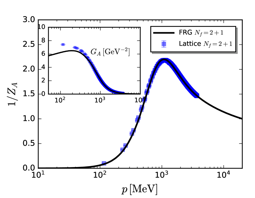
Figure 3: $N_{f}=2+1$ gluon dressing function $1/Z_{A}(p^{2})$ and gluon propagator $G_{A}=1/[Z_{A}(p^{2})\,p^{2}]$ (inset) in the vacuum as functions of momenta in comparison to lattice results based on the $N_{f}=2+1$ configurations (domain wall fermions) of the RBC/UKQCD collaboration, e.g. Blum et al. (2016). The lattice results are continuum extrapolated from data with $\beta=2.25,\,a^{-1}=2.359(7)\,\textrm{GeV},\,m_{\pi}=139.2(5)$ MeV and $\beta=2.13,\,a^{-1}=1.730(4)\,\textrm{GeV},\,m_{\pi}=139.2(4)$ MeV, see Zafeiropoulos et al. (2019); Boucaud et al. (2018, 2019). The momentum dependence of the fRG results is given by $p^{2}=k^{2}$, in accordance with the same identification of the $N_{f}=2$ flavour input data; for more details see Section IV.1.2.

Strictly speaking, absolute momentum scales should be measured in the pion decay constant in the chiral limit. In the present approximation it is computed as

$$f_{\pi,\chi}=88.6\,\textrm{MeV}\quad\textrm{for}\quad N_{f}=2+1\,,$$ (53)

see (195). The details of the scale setting procedure are discussed in Appendix E.3. Apart from the quantitative precision of the predictions for observables in Table 1 in particular for $N_{f}=2+1$, the $N_{f}=2+1$ gluon dressing is a prediction within the current setup. It agrees quantitatively with the respective lattice results, see Figure 3. Note that the gluon propagator shows the expected deviations in the deep infrared: the $N_{f}=2$ flavour propagator in Cyrol et al. (2018a) is of the scaling type, related to a different infrared closure of the Landau gauge as that implicitly defined by the lattice gauge fixing. This has been discussed at length in the literature, see Cyrol et al. (2018a) and references therein. Importantly, as part of the gauge fixing, it has no impact on observables.

III.4 Strong couplings $\alpha_{s}$ from gluon, ghost-gluon and quark-gluon vertices

The quark-gluon and purely gluonic correlation functions in the current approximation give rise to different ‘avatars’ of the strong couplings $\alpha_{\Phi_{1}\cdots\Phi_{n}}$ with $\Phi_{i}=A_{\mu},c,\bar{c},q,\bar{q}$ and $n=3,4$. For details see Mitter et al. (2015); Cyrol et al. (2016, 2018a, 2018b), for similar considerations in quantum gravity see Eichhorn et al. (2018, 2019). They are defined by the respective vertex dressings $\lambda_{\Phi_{1}\cdots\Phi_{n}}$, divided by the wave function renormalisations $\prod Z_{\Phi_{i}}^{1/2}$ of the attached legs evaluated at vanishing momentum, see e.g. Cyrol et al. (2018a). Here we consider the couplings of the purely gluonic sector,

$$\alpha_{A^{3}}=\frac{1}{4\pi}\frac{\lambda_{A^{3}}^{2}}{Z_{A}^{3}}\,,\quad\alpha_{A^{4}}=\frac{1}{4\pi}\frac{\lambda_{A^{4}}}{Z_{A}^{2}}\,,\quad\alpha_{\bar{c}Ac}=\frac{1}{4\pi}\frac{\lambda_{Ac\bar{c}}^{2}}{Z_{A}\,Z_{c}^{2}}\,,$$ (54)

and that of the matter sector, $\alpha_{\bar{q}Aq}=(\alpha_{\bar{l}Al},\alpha_{\bar{s}Ac})$ with two entries for the light quark-gluon and strange quark-gluon couplings respectively,

$$\alpha^{\ }_{\bar{l}Al}=\frac{1}{4\pi}\frac{\lambda_{Al\bar{l}}^{2}}{Z_{A}\,Z_{l}^{2}}\,,\qquad\alpha_{\bar{s}As}=\frac{1}{4\pi}\frac{\lambda_{As\bar{s}}^{2}}{Z_{A}\,Z_{s}^{2}}\,.$$ (55)

Note that the strong couplings (54), (55) are natural definitions of gluon exchange couplings. For example, the quark-gluon couplings involve two quark-gluon vertex functions and one gluon dressing $1/Z_{A}$, related to the one-gluon scattering of two quark currents, see Figure 4.

For perturbative and semiperturbative scales $k\gtrsim 1-3\,$GeV these couplings are related by modified Slavnov-Taylor identities (mSTIs). This property also holds true in the quantitative approximation Mitter et al. (2015); Cyrol et al. (2016, 2018a, 2018b) for the purely gluonic couplings, for more details see in particular Cyrol et al. (2018a). We emphasise that in the present setup gauge invariance is encoded in these mSTIs. They arise from BRST-variations of the gauge fixed action in the presence of the regulator terms, see e.g. Ellwanger (1994b); Bonini et al. (1995); D’Attanasio and Morris (1996); Becchi (1996); Reuter and Wetterich (1997); Freire et al. (2000); Igarashi et al. (2001); Pawlowski (2003, 2007); Wetterich (2018); Igarashi et al. (2019). For smaller momenta and cutoff scales $k\lesssim 1-3\,$GeV they start to differ for two reasons: first of all the gluon mass scale starts to influence the running. More importantly the mSTIs only relate the longitudinal couplings, while the flow depends on the transversal couplings. It can be shown that some of the transversal $\alpha$’s cannot be identified with their longitudinal counterparts as otherwise the gluon mass scale would be absent, see Cyrol et al. (2016); Cornwall (1982); Aguilar et al. (2011, 2012, 2019). However, in the absence of the gluon mass scale in the propagator the theory lacks confinement, Braun et al. (2010a, b); Fister and Pawlowski (2013).

Here we compute the flows of the three-gluon coupling, $\alpha_{A^{3}}$, and the quark-gluon couplings $\alpha_{\bar{q}Aq}$. From the vacuum results for the couplings in Braun et al. (2016a); Cyrol et al. (2018a) we infer that the four-gluon coupling runs closely to $\alpha_{A^{3}}$, and the ghost-gluon coupling runs closely to $\alpha_{\bar{q}Aq}$ in the relevant momentum regime $k\gtrsim 1$  GeV. In the deep infrared all these couplings. However, except of the ghost-gluon coupling, all the avatars of the strong coupling decay for these scales, see Figure 17 in Section IV.2.3, and Braun et al. (2016a); Cyrol et al. (2018a). The ghost-gluon coupling only enters in diagrams that are suppressed except for the deep infrared with $k\lesssim 100$ MeV, a more detailed discussion of this fact is provided in Section IV.2.2. In summary the differences lead to negligible effects and we use

$$\alpha_{A^{4}}=\alpha_{A^{3}}=\alpha_{\textrm{glue}}\,,\qquad\alpha_{\bar{c}Ac}\simeq\alpha_{\bar{q}Aq}\,.$$ (56)

For gluons and quarks this leads us to covariant derivatives in the fundamental and adjoint representation of $SU(N_{c})$ respectively,

$$D_{\mu} =\partial_{\mu}-iZ_{A}^{1/2}g_{\bar{q}Aq}A^{a}_{\mu}t^{a}\,,$$

$$D^{ab}_{\mu} =\partial_{\mu}\delta^{ab}-Z_{A}^{1/2}g_{\textrm{\tiny{glue}}}f^{abc}A^{c}_{\mu}\,,$$ (57)

where

$$g_{\textrm{\tiny{glue}}}=\sqrt{4\pi{\alpha}_{\textrm{\tiny{glue}}}}\,,\qquad g_{\bar{q}Aq}=\sqrt{4\pi{\alpha}_{\bar{q}Aq}}\,.$$ (58)

The covariant derivative in the ghost terms is an adjoint one but carries $g_{\bar{q}Aq}$. In (57), $f^{abc}$ are the structure constants for the $SU(N_{c})$ group with

$$[t^{a},t^{b}]=if^{abc}t^{c}\,,\qquad\qquad\operatorname{Tr}\,t^{a}t^{b}=\frac{1}{2}\delta^{ab}\,.$$ (59)

The terms in the first two lines on the r.h.s. of (39) are built from the operators in the classical QCD action. The gluonic field strength tensor reads

$$F^{a}_{\mu\nu} =Z_{A}^{1/2}\left(\partial_{\mu}A^{a}_{\nu}-\partial_{\nu}A^{a}_{\mu}+Z_{A}^{1/2}g_{\textrm{\tiny{glue}}}f^{abc}A^{b}_{\mu}A^{c}_{\nu}\right)\,,$$ (60)

and the Landau gauge $\xi=0$ is chosen in this work.

A similar truncation has been found to be successful in describing the transition from the quark-gluon regime at high energy to the hadronic one at low energy in the vacuum Braun et al. (2016a). The truncation (39) for the effective action takes into account all order scatterings of the resonant scalar and pseudoscalar channels of the four-fermi interaction through the scale-dependent effective potential $V_{k}(\rho,L,\bar{L})$. It is complementary to taking into account a Fierz-complete four-fermi basis as done in Mitter et al. (2015); Cyrol et al. (2018a); Braun et al. (2017, 2018); Leonhardt et al. (2019). A respective two flavour study with a Fierz complete basis and all order interactions of resonant channels is work in progress, Braun et al. .

III.5 Dynamical hadronisation in the $\sigma-\pi$ channel

As discussed in Section II, we take into account the resonant interactions in the $\sigma-\bm{\pi}$ channel with the help of dynamical hadronisation. We use (15) with ${\dot{B}}_{k}=0$, ${\dot{C}}_{k}=0$,

$$\langle\partial_{t}\hat{\phi}_{k}\rangle= \dot{A}_{k}\,\bar{q}\tau q\,,$$ (61)

in the flow equation (26). Our strategy is to choose the coefficients in (61) such that the running of the four-quark interaction $\lambda_{q}$ in (39) is exactly cancelled. This amounts to a scale dependent bosonisation of this channel. We emphasise that this only transfers the information carried by four-quark interaction from the quark-gluon sector to the meson sector. It is a practical way to enter the symmetry broken phase in the presence of resonant channels and still retain the full information of the underlying dynamics of the fundamental degrees of freedom. In case of the scalar-pseudoscalar channel considered here, a resonance at vanishing momentum indicates the formation of a quark condensate $\langle\bar{q}q\rangle$ and therefore chiral symmetry breaking.

Figure 4: Flow equation for the four-quark coupling in the present approximation. Further diagrams with the nonresonant part of the scalar-pseudoscalar channel and other four-quark tensor structures, as well as that with higher order couplings are dropped. The black dots denote the full vertices and the various lines represent for the full propagators. The derivative $\tilde{\partial}_{t}=\left.\partial_{t}\right|_{\{\Gamma^{(n)}_{k}\}}$ only hits the $k$-dependence of the regulator, e.g. $\tilde{\partial}_{t}G_{k}=-G_{k}\dot{R}_{k}G_{k}$. The first line with the quark-gluon diagrams generates the four-quark interaction through gluon-exchange at large scales. The second line takes into account the self-interaction of the resonant four-quark interaction in terms of meson exchange diagrams. The last line comprises the mixed diagrams with meson and gluon exchange. Gluon-exchange dominates the flow for large and intermediate energy scales, while the meson-exchange diagrams dominate at low energy, see Appendix L. Accordingly, in the present work we keep the quark-gluon and quark-meson diagrams and drop the mixed ones.

To this end, we project the flow equation on the flow of the scalar-pseudoscalar four-quark vertex, $\lambda_{q}$ in (39) at vanishing momentum. We define the respective dimensionless, renormalised four-quark coupling, Yukawa coupling and hadronisation function as

$$\bar{\lambda}_{q}=\frac{\lambda_{q}\,k^{2}}{Z_{q}^{2}}\,,\qquad\bar{h}=\frac{h}{Z_{\phi}^{1/2}Z_{q}}\,,\qquad\dot{\bar{A}}=\frac{Z_{\phi}^{1/2}}{Z_{q}}\dot{A}\,k^{2}\,,$$ (62)

where we suppressed the subscript $k$, and the renormalised Yukawa coupling has already been introduced in (43). With these definitions the flow of the renormalised four-quark function reads

$$\partial_{t}\bar{\lambda}_{q}-2\left(1+\eta_{q}\right)\bar{\lambda}_{q}-\bar{h}\,\dot{\bar{A}}=\overline{\textrm{Flow}}^{(4)}_{(\bar{q}\tau q)(\bar{q}\tau q)}\,,$$ (63)

where

$$\overline{\textrm{Flow}}^{(n)}_{\Phi_{i_{1}}\cdots\Phi_{i_{n}}}=\frac{1}{\prod_{j=1}^{n}Z^{1/2}_{{\Phi_{i_{j}}}}\,k^{d_{\lambda_{{\Phi_{i_{1}}\cdots\Phi_{i_{n}}}}}}}\textrm{Flow}^{(4)}_{\Phi_{i_{1}}\cdots\Phi_{i_{n}}}\,,$$ (64)

are the dimensionless, renormalised flow diagrams.

The projection on the scalar-pseudoscalar four-quark channel in (64) is done along the lines of Braun (2012) with an expansion of the flow in terms of quark-bilinears. This is indicated by the subscript ${}_{(\bar{q}\tau q)(\bar{q}\tau q)}$. $\textrm{Flow}^{(n)}$ is defined in (38), and $d_{\lambda_{{\Phi_{i_{1}}\cdots\Phi_{i_{n}}}}}$ is the canonical momentum dimension of the vertex dressing $\lambda_{\Phi_{i_{1}}\cdots\Phi_{i_{n}}}$. Now we resort to fully hadronised flows in the $\sigma$–$\bm{\pi}$ channel by demanding

$$\bar{\lambda}_{q}\equiv 0\,,\qquad\forall k\,.$$ (65)

With this, all diagrams with four-quark vertices $\bar{\lambda}_{q}$ are absent and the flow is depicted by Figure 4. The diagrams in the first line on the r.h.s. in Figure 4 arise from the exchange of gluons and those in the second line from mesons. The respective expressions are given in Appendix L, (220) and (221). The mixed diagrams with gluon and meson exchange, shown in the third line in Figure 4, are neglected here, since the dynamics of gluons and mesons dominate in approximately disjoint regions of the RG scale and the mixed diagrams are comparatively small in either regime, cf. Appendix L.

Inserting (65) into (63) leaves us with an equation for the hadronisation function,

$$\dot{\bar{A}} =-\frac{1}{\bar{h}}\,\overline{\textrm{Flow}}^{(4)}_{(\bar{q}\tau q)(\bar{q}\tau q)}\,.$$ (66)

This choice entails that the quantum fluctuations contributing to the quark scattering in the $\sigma$–$\bm{\pi}$ channel are transferred completely to effective hadronic degrees of freedom, the $\sigma$ and $\bm{\pi}$ fields, their propagation, self-scattering and scattering with quark-antiquark pairs.

The original four-quark interaction is described with instantaneous meson propagators and a Yukawa interaction of the $\sigma,\bm{\pi}$ with a quark-antiquark pair. Multi-scatterings of the resonant channels are encoded in the effective potential $V_{k}$. The flow of the respective couplings and propagators is discussed in Section IV.

III.6 Thermodynamic potential & order parameters

The equilibrium thermodynamic potential density $\Omega$ is given by

$$\Omega[\Phi;T,\mu] =\Big{(}\frac{T}{\cal V}\Big{)}\Gamma_{k=0}[\Phi]\,,$$ (67)

where $\cal V$ is the spatial volume. $\Omega[\Phi;T,\mu]$ is nothing but $V_{k=0}(\rho,L,\bar{L})$ in (40). It depends on the given background $\Phi$, the temperature $T$ and the quark chemical potential $\mu$. In the present case we only consider homogeneous background fields and the infinite volume limit. Equation (67) can be obtained from the evolution of the effective action $\Gamma_{k}$ with (26). To simplify the calculations, we split $\Gamma_{k}$ into two parts,

$$\Gamma_{k}[\Phi]=\Gamma_{\text{\tiny{glue}},k}[\Phi]+\Gamma_{\text{\tiny{matt}},k}[\Phi]\,,$$ (68)

where the glue sector corresponds to the first two loops in Figure 2, and the matter sector to the latter two. The thermodynamic potentials related to the two parts are dealt with differently in this work; that is, we do not evolve the flow of $\Gamma_{\text{\tiny{glue}},k}$, but instead replace it with the QCD-enhanced glue potential Haas et al. (2013); Herbst et al. (2014), to wit,

$$\Big{(}\frac{T}{\cal V}\Big{)}\Gamma_{\text{\tiny{glue}},k=0}[\Phi]=V_{\text{\tiny{glue}}}(L,\bar{L})\,.$$ (69)

In (69) we have introduced the traced Polyakov loops $L,\bar{L}$ with

$$L(\bm{x})=\frac{1}{N_{c}}\left\langle\operatorname{Tr}\,{\cal P}(\bm{x})\right\rangle\,,\quad\bar{L}(\bm{x})=\frac{1}{N_{c}}\langle\operatorname{Tr}\,{\cal P}^{\dagger}(\bm{x})\rangle\,,$$ (70)

and

$${\cal P}(\bm{x})=\mathcal{P}\exp\Big{(}ig\int_{0}^{\beta}d\tau\hat{A}_{0}(\bm{x},\tau)\Big{)}\,.$$ (71)

Here, $\mathcal{P}$ on the r.h.s. standing for the path ordering. In (71) the gauge field is the fluctuation field and $A_{0}=\langle\hat{A}_{0}\rangle$ is the temporal mean gauge field in $\Phi$. Accordingly, the expectation values (70) are nontrivial functions of the mean field $A_{0}$ and

$$L[A_{0}]\neq\frac{1}{N_{c}}\operatorname{Tr}\,{\cal P}[A_{0}]\,.$$ (72)

This has been discussed at length in Braun et al. (2010a); Marhauser and Pawlowski (2008); Braun et al. (2010b); Fister and Pawlowski (2013); Herbst et al. (2015), for related work see e.g. Fukushima and Skokov (2017); Fukushima and Kashiwa (2013); Reinosa et al. (2015a, b); Maelger et al. (2018a, b).

However, in Herbst et al. (2015) it has been shown that the difference in (72) can largely be attributed to a temperature-dependent rescaling.

In the present work this difference is ignored, it will be discussed elsewhere. We approximate $L[A_{0}]\approx\frac{1}{N_{c}}\operatorname{Tr}\,{\cal P}[A_{0}]$ which allows us to utilise pure glue lattice results for the expectation value $L$ and the correlations of the Polyakov loop for the construction of the Polyakov loop potential. The glue potential $V_{\text{\tiny{glue}}}$ employed in this work is that computed in Lo et al. (2013), where the quadratic fluctuations of the Polyakov loop, $\langle{\cal P}[A_{0}](\bm{x}){\cal P}[A_{0}](\bm{y})\rangle$, are taken into account. We specify the glue potential in Appendix G. Finally, one obtains the thermodynamic potential density as follows

$$\Omega[\Phi;T,\mu] =V_{\text{\tiny{glue}}}(L,\bar{L})+V_{\text{mat}}(\rho,L,\bar{L})-c_{\sigma}\sigma\,.$$ (73)

The potential (73) allows us to access both, the confinement-deconfinement phase transition or crossover via the Polyakov loop expectation value $L$,

$$\left.\frac{\partial\Omega[\Phi;T,\mu]}{\partial L}\right|_{\Phi=\Phi_{\textrm{EoM}}}=\left.\frac{\partial\Omega[\Phi;T,\mu]}{\partial\bar{L}}\right|_{\Phi=\Phi_{\textrm{EoM}}}=0\,,$$ (74)

where $\Phi_{\textrm{EoM}}$ now includes $L_{\textrm{EoM}},\bar{L}_{\textrm{EoM}}$ instead of $A_{0,\textrm{EoM}}$ in a slight abuse of notation.

In turn, explicit and spontaneous chiral symmetry breaking is encoded in the expectation value $\langle\sigma\rangle:=\sigma_{\textrm{EoM}}$ of the $\sigma$-field, defined with the respective EoM,

$$\left.\frac{\partial V_{k=0}(\rho,L,\bar{L})}{\partial\sigma}\right|_{\Phi_{\textrm{EoM}}}=c_{\sigma}\,.$$ (75)

The expectation value $\sigma_{\textrm{EoM}}$ is an order parameter for chiral symmetry breaking similar to the magnetisation in the Ising model. It is closely related to the chiral condensate of the light quarks, $\langle\bar{u}u+\bar{d}d\rangle/2$, which is a function of the constituent quark mass of the light flavours,

$$\bar{m}_{l}=\frac{1}{2}\,\bar{h}\bar{\sigma}_{\textrm{EoM}}\,.$$ (76)

The potential (73) also gives us access to the thermodynamics of the system which will be discussed elsewhere.

IV Correlation functions

In this section we discuss the correlation functions presented in (39), and derive their flow equations. This includes the propagators of all fields and the respective anomalous dimensions (Section IV.1), the strong couplings related to pure glue, ghost-gluon and quark-gluon vertices (Sections IV.2.2, IV.2.1), the four-quark scattering and the Yukawa coupling between pions, $\sigma$ and the quarks due to dynamical hadronisation (Section IV.3), and the flow of the effective potential (Section IV.4).

IV.1 Propagators and anomalous dimensions

The flow equation for the (inverse) propagators, $\partial_{t}\Gamma^{(2)}_{k}(p)$ is obtained by taking the second derivative w.r.t. the fields of the Wetterich equation (26). They are depicted in Figure 5 for the quark, gluon, and meson fields, respectively. We are led to the anomalous dimensions $\eta_{\Phi_{i}}$ with $\Phi_{i}=(A,q,\bar{q},\phi)$. While the $\eta_{A}$ comprises the full flow of the inverse gluon propagator, the mass terms of quarks and mesons are field dependent. They are captured by the Yukawa term and the second derivative of the effective potential respectively.

IV.1.1 Mesons and quarks

The full quark and meson two-point functions (at vanishing pion fields $\bm{\pi}=0$ and vanishing quark chemical potential $\mu_{q}=0$) are given by

$$\Gamma^{(2)}_{q\bar{q}}(p)= \,Z_{q}(p)\,\left[ip\hbox to0.0pt{\hss/}+M_{q}(p)\right]\,,$$

$$\Gamma^{(2)}_{\phi\phi}(p)= \,Z_{\phi}(p)\,p^{2}+m_{\phi}^{2}\,,$$ (77)

where both the wave function renormalisations and the mass terms also depend on the chosen mesonic field $\phi$. The notation in (77) is that in Mitter et al. (2015); Cyrol et al. (2018a), where the full momentum dependence of the meson and quark two-point function of two-flavour QCD in the vacuum has been computed. The running quark mass parameter in the present work is given by $\bar{m}_{l,k}=M_{l,k}(0)$, and this relation holds on a quantitative level, see the Figures 26 and 28 in Appendix E.3. Evidently, the fully momentum-dependent wave function renormalisations $Z_{q}(p)$ and mass functions $M_{q}(p)$ of the quarks are uniquely defined as the prefactor of the Dirac tensor structure and the scalar tensor structure respectively,

$$Z_{q_{i}}(p)= \,\frac{1}{4N_{c}}\frac{1}{p^{2}}\operatorname{tr}p\hbox to0.0pt{\hss/}\,\Gamma^{(2)}_{q_{i}\bar{q}_{i}}(p)\,,$$

$$M_{q_{i}}(p)= \,\frac{1}{4N_{c}}\frac{1}{Z_{q_{i}}(p)}\operatorname{tr}\Gamma^{(2)}_{q_{i}\bar{q}_{i}}(p)\,,$$ (78)

where $\operatorname{tr}$ stands for the Dirac and colour trace, and we do not sum over the flavour index $i=1,...,3$. The different tensor structures for the kinetic term and the mass term provide us also with unique projections of the flow equation on the flows $\partial_{t}Z_{q}(p)$ and $\partial_{t}M_{q}(p)$ respectively. The latter flow is related to the flow of the Yukawa coupling and is discussed in Chapter IV.3. The flow of the wave function renormalisation is encoded in the anomalous dimension (30) of the quarks. In the present work we do not introduce a thermal splitting of the wave function renormalisation in parts longitudinal and transversal to the heat bath, but use the transversal part throughout. This leads us to

$$\eta_{q_{i}}(p_{0},\bm{p})=\frac{1}{4N_{c}}\frac{1}{Z_{q,k}(p_{0},\bm{p})}\mathrm{Re}\left[\frac{i}{\bm{p}^{2}}\mathrm{tr}\,\bm{\gamma}\cdot\bm{p}\,\partial_{t}\Gamma^{(2)}_{\bar{q}_{i}q_{i},k}(p)\right]\,,$$ (79)

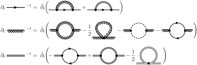
Figure 5: Flow equations for the inverse propagators of quarks, gluons, mesons respectively, in the present approximation; in particular the tadpole contribution from two-quark–two-meson as well as the remnant four-quark scatterings are missing, as is the ghost-gluon tadpole. The derivative $\tilde{\partial}_{t}$ is defined in the caption of Figure 4. The left hand sides stand for, in a slight abuse of notation, $\partial_{t}\Gamma_{k}^{(2)}=\partial_{t}\left(G_{k}^{-1}-R_{k}\right)$, where we have dropped the $-R_{k}$ in the depiction.

where no sum over the flavours $i$ is taken. It is well-known that the anomalous dimension of the quark carries a mild momentum dependence, for results in the present fRG setting as well as respective DSE and lattice results see Mitter et al. (2015); Cyrol et al. (2018a); Williams et al. (2016); Fischer (2019). In particular, from Mitter et al. (2015); Cyrol et al. (2018a) we infer a very small momentum dependence of $\eta_{q}$ in the regime $p^{2}\leq k^{2}$. Hence, we use $\bm{p}=0$ which facilitates the explicit expressions,

$$\eta_{q_{i}}(p_{0})=\frac{1}{4\,Z_{q_{i},k}(p_{0})}\mathrm{Re}\left[i\frac{\partial}{\partial\bm{p}^{2}}\mathrm{tr}\,\bm{\gamma}\cdot\bm{p}\,\partial_{t}\Gamma^{(2)}_{\bar{q}_{i}q_{i},k}(p)\right]_{\bm{p}=0}\,,$$ (80)

where $p_{0}$ is a small, but nonvanishing, frequency, for more details see Appendix J. Its nontrivial choice is also related to fact that the expression in the square bracket is complex for nonvanishing chemical potential. This is well-understood and originates in the Silver-Blaze property: At vanishing temperature correlation functions involving a quark field $q(\omega)$ below density onset are real functions of the complex frequency variable $\omega-i\,\mu_{q}$, for a detailed discussion in the fRG and 2PI approaches see Markó et al. (2014); Khan et al. (2015); Fu and Pawlowski (2016). Therefore we project the flow on its real part, denoted by $\mathrm{Re}$. The trace in (80) projects on the Dirac tensor structure in the quark two-point function, that is its kinetic part. The explicit expression of $\eta_{q,k}$ is also given in Appendix J.

It follows from the parameterisation (77) that the mesonic wave function renormalisations and masses are given by

$$Z_{\phi}(p)= \,\frac{1}{p^{2}}\left[\Gamma_{\phi\phi}^{(2)}(p^{2})-\Gamma_{\phi\phi}^{(2)}(0)\right]\,,$$

$$m_{\phi}^{2}= \,\Gamma_{\phi\phi}^{(2)}(0)\,.$$ (81)

In contradistinction to the quark wave function renormalisations and masses, that of the mesonic degrees of freedom do not allow for unique definitions as they cannot be distinguished by their tensor structures. Accordingly, one can easily shift momentum dependence from the wave function renormalisation $Z_{\phi}$ to the mass $m_{\phi}^{2}$ in (77). Furthermore, for given $\phi_{0}=(\sigma_{0},\bm{\pi}=0)$, the $\sigma$ and $\bm{\pi}$ parts of $\Gamma^{(2)}_{\phi\phi}$ are different,

$$\Gamma^{(2)}_{\sigma\sigma}(p)= \,Z_{\sigma,k}(p)\,p^{2}+m_{\sigma}^{2}\,,$$

$$\Gamma^{(2)}_{\pi_{i}\pi_{i}}(p)= \,Z_{\pi,k}(p)\,p^{2}+m_{\pi}^{2}\,.$$ (82)

The $\sigma$ and pion masses are given by the curvature of the mesonic potential $V_{k}$ in the respective field directions,

$$m_{\pi}^{2}=\partial_{\rho}V_{k}\,, m_{\sigma}^{2}=m_{\pi}^{2}+2\rho\,\partial_{\rho}^{2}V_{k}\,,$$ (83)

and are hence called curvature masses, see e.g. Helmboldt et al. (2015). Evidently, the pion mass vanishes in the chiral limit as it is simply given by the EoM for $c_{\sigma}=0$. The two masses differ by a higher $\rho$-derivative term which is only present for $\rho_{0}\neq 0$, that is $\sigma_{0}\neq 0$ as $\bm{\pi}\equiv 0$. The wave function renormalisations follow similarly,

$$Z_{\pi}(p)=Z_{\phi}(p)\,, Z_{\sigma}(p)=Z_{\phi}(p)+\rho\partial_{\rho}Z_{\phi}(p)\,.$$ (84)

In the present approximation we do not consider the dependence of the wave function renormalisations on the mesonic fields. These terms amount to momentum-dependent mesonic self-scatterings that vanish at vanishing momentum. These terms are suppressed at low energies which is the only regime where the offshell mesonic fluctuations can play a r$\hat{\textrm{o}}$le in the first place. This leaves us with a uniform wave function renormalisation which we define via the pion two-point function,

$$Z_{\phi}(p)=Z_{\pi}(p)\,.$$ (85)

A natural definition of $Z_{\pi}$ comes from the definition of the pion pole mass

$$\bar{\Gamma}^{(2)}_{\pi_{i}\pi_{i}}(p_{0}=im_{\pi,\textrm{pol}},\,\bm{p}^{2}=0)=0\,,$$ (86)

with $\bar{\Gamma}^{(2)}_{\phi\phi}(p_{0},\bm{p})=\Gamma_{\phi\phi}^{(2)}(p_{0},\bm{p})/Z_{\phi}(p_{0},\bm{p})$, which implies

$$m_{\pi,\textrm{pol}}^{2}=\frac{1}{Z_{\pi}(im_{\pi,\textrm{pol}},0)}m_{\pi}^{2}\,,$$ (87)

see e.g. Helmboldt et al. (2015). In the present Euclidean setup we are restricted to $p_{0}^{2}\geq 0$. The approximation $Z_{\pi}(im_{\pi,\textrm{pol}},0)\approx Z_{\pi}(0,0)\equiv Z_{\pi}(0)$ is therefore the optimal choice for the wave function renormalisation in (87), as it is closest to the pion pole. Since this pole, in turn, is close to the origin in the region where mesons are dynamically relevant, this approximation is even quantitative if $Z_{\pi}(p)$ is only mildly momentum dependent in the small region $|p^{2}|\lesssim m_{\pi}^{2}$. Indeed, this has been demonstrated to be true for cutoffs $\lesssim 1$ GeV within low energy effective theories in Helmboldt et al. (2015). Hence, we arrive at

$$m_{\pi,\textrm{pol}}^{2}=\frac{1}{Z_{\pi}(0)}m_{\pi}^{2}\,,$$ (88)

which also implies that the pole mass and the (renormalised) curvature mass of the pion agree. Therefore we consider explicitly the pion wave function renormalisation, and with (85) we arrive at

$$Z_{\phi}(p)=\frac{1}{3}\delta_{ij}\frac{1}{p^{2}}\left[\Gamma^{(2)}_{\pi_{i}\pi_{j}}(p)-\Gamma^{(2)}_{\pi_{i}\pi_{j}}(0)\right]\,.$$ (89)

For momenta close to the pion pole this agrees well with the pole renormalisation. In the present work we consider $p^{2}\geq 0$ and hence the optimal choice is $\bm{p}^{2}=0$ and $p_{0}=0$, where the latter limit is taken first. This leads us to

$$Z_{\phi}(0)=\frac{1}{3}\delta_{ij}\left[\frac{\partial\Gamma^{(2)}_{\pi_{i}\pi_{j}}}{\partial\bm{p}^{2}}\right](p=0)\,,$$ (90)

with the pion pole mass (88). As for the quarks we have neglected the thermal splitting of the wave function renormalisation in parts longitudinal and transversal to the heat bath. Instead we use the transversal part throughout. The validity of this approximation has been checked explicitly in e.g. Yin et al. (2019).

In the present work we also approximate the full momentum dependence of the quark and meson propagators in the diagrams by cutoff-scale–dependent wave function renormalisations and masses. The cutoff scale dependence carries the -averaged- momentum dependence at $p^{2}\approx k^{2}$. Accordingly, this approximation provides even semiquantitative results in the flow if the momentum dependence of the propagators is small for momenta $p^{2}\lesssim k^{2}$. Moreover, the spatial momentum $\bm{q}$ loop integrals of flows of correlation functions at vanishing external spatial momenta $\bm{p}_{i}=0$ are peaked at $\bm{q}^{2}\approx k^{2}$ for generic cutoffs, and $\bm{q}^{2}=k^{2}$ for the present cutoff choice. Both properties originate in the spatial momentum measure

$$\int\frac{d^{3}q}{(2\pi)^{3}}\,{\cal I}_{k}(\bm{q}^{2})=\frac{1}{2\pi^{2}}\int_{0}^{\infty}dq\,q^{2}\,{\cal I}_{k}(q^{2})\,,$$ (91)

with ${\cal I}_{k}({q}^{2}>k^{2})=0$ for the present cutoff choice (225). We conclude that if approximating the full $Z_{\phi}(p)$ with (89) at $p=k$, the flow diagrams with meson propagators are well-approximated. This leads us to the following approximation of the full momentum dependence of the meson two point function in the right hand side of the flow equations,

$$\Gamma^{(2)}_{\phi\phi}(p)= \,\bar{Z}_{\phi,k}\,p^{2}+m_{\phi}^{2}\,,$$

$$\partial_{t}\bar{Z}_{\phi,k}= \,\frac{\partial_{t}\Gamma^{(2)}_{\phi\phi}(0,k)-\partial_{t}\Gamma^{(2)}_{\phi\phi}(0)}{k^{2}}\,,$$ (92)

where $(0,k)$ stands for $(p_{0}=0,\bm{p}^{2}=k^{2})$. In summary, best use of these consideration is made if $\bar{Z}_{\phi}$ with (92) is used in the flow diagrams, while $Z_{\phi}(0)$ defined in (90) is used for determining the current quark masses via the pole mass of the pion in the vacuum.

It is left to derive the flow equations for the wave function renormalisations $\bar{Z}_{\phi}$ and $Z_{\phi}(0)$. Both can be read of from the anomalous dimension (30) computed from the $k$-derivative of (89). We use that

$$\eta_{\phi}(0,\bm{p})=-\frac{\delta_{ij}}{3Z_{\phi}(0,\bm{p})}\frac{\partial_{t}\Gamma_{\pi_{i}\pi_{j}}^{(2)}(0,\bm{p})-\partial_{t}\Gamma_{\pi_{i}\pi_{j}}^{(2)}(0,\bm{p})}{\bm{p}^{2}}\,,$$ (93)

lead to the flow of $\bar{Z}_{\phi}$ with

$$\frac{1}{\bar{Z}_{\phi}}\partial_{t}\bar{Z}_{\phi}:=-\eta_{\phi}(0,k)\,,\quad\textrm{with}\quad\bar{Z}_{\phi,\Lambda}=Z_{\phi,\Lambda}\equiv 1\,.$$ (94)

Note that (93) and (94) imply that $\bar{Z}_{\phi}\neq Z_{\phi}(0,k)$. This can be seen from the $t$-derivative of $Z_{\phi}(0,k)$,

$$\partial_{t}\left[\log Z_{\phi}(0,k)\right]=-\eta_{\phi}(0,k)+\frac{k}{Z_{\phi}(0,k)}\frac{\partial Z_{\phi}}{\partial|\bm{p}|}(0,k)\,,$$ (95)

where the second term comes from the spatial momentum $|\bm{p}|=k$ in $Z_{\phi}(0,k)$. We emphasise again that the present approximation is based on the mild momentum dependence of the mesonic wave function renormalisation for $p^{2}\lesssim k^{2}$ of both low energy effective theories as well as full QCD. In the vacuum this has been shown in Helmboldt et al. (2015); Mitter et al. (2015); Cyrol et al. (2018a). Note, however, that at finite density a nontrivial momentum dependence of the meson wave function renormalisation can be induced by a modulated spatial structure, e.g. due to an inhomogeneous quark condensate. As discussed below, we find indications for such a regime here.

For the determination of the pion mass in the vacuum we also require the wave function renormalisation at vanishing momentum, $Z_{\phi}(0)$. Its flow is read-off from (90),

$$\eta_{\phi}(0) =-\frac{1}{3Z_{\phi}(0)}\delta_{ij}\left[\frac{\partial}{\partial\bm{p}^{2}}\partial_{t}\Gamma^{(2)}_{\pi_{i}\pi_{j}}\right](p=0)\,.$$ (96)

The explicit expression for (93) and (96) are deferred to Appendix I. Note that $Z_{\phi}(0)$ and $Z_{\phi}(0,k)$ agree at $k=0$, while $\bar{Z}_{\phi}$ does not. This deviation can be used for a systematic error estimate, since the wave function renormalisations only enter via $\eta_{\phi}$. Accordingly, it is the difference $\eta_{\phi}(0,k)+\partial_{t}\ln Z_{\phi}(0,k)$, that is the last term on the right hand side of (95), which is missing in the flows. We have checked numerically that this difference does not play any r$\hat{\textrm{o}}$le.

In the current approximation, the pion pole mass in the vacuum is given by

$$m_{\pi,\text{pol}}=\frac{m_{\pi}}{\sqrt{Z_{\phi,k=0}(0)}}\,.$$ (97)

Similarly we approximate

$$m_{\sigma,\text{pol}}\approx\frac{m_{\sigma}}{\sqrt{Z_{\phi,k=0}(0)}}\,.$$ (98)

However, we emphasise that (98) carries a qualitatively larger systematic error in comparison to (97): Apart from the fact that the physical meaning of the $\sigma$-resonance in the scalar four-quark channel is still debated, Jaffe (1977a, b), it requires a small momentum behaviour for a larger momentum range $|p^{2}|\lesssim m_{\sigma,\text{pol}}^{2}$. Nonetheless, in an extension of the current setup to Minkowski frequencies the respective observable provides the position of the lowest resonance in the scalar channel.

Within this setup we adjust the pion mass in the vacuum, $m_{\pi,\textrm{pol}}=137$ MeV, by fixing $c_{\sigma}$. For the systematic error estimate we also have run the vacuum flows with $\eta_{\phi}(0)$ instead of $\eta_{\phi}(0,k)$. Starting from the same initial conditions we get a pion pole mass of 140 MeV, which gives us a $\sim 2\%$ error. Moreover, the purely fermionic observables, e.g. for $N_{f}=2+1$ the constituent light quark mass $\bar{m}_{l}\!=\!347$ MeV ($\eta_{\phi}(0,k)$), 343 MeV ($\eta_{\phi}(0)$) and the four fermion coupling $\bar{h}_{k}^{2}/(2\bar{m}_{\pi,k}^{2})\!=\!2.73\times 10^{3}\,\text{GeV}^{-2}$ ($\eta_{\phi}(0,k)$), $2.80\times 10^{3}\,\text{GeV}^{-2}$ ($\eta_{\phi}(0)$) also give us a systematic error estimate of $\lesssim 2$ %. Technically, this stability of the fermionic observables comes about as $\eta_{\phi}$ plays a subleading r$\hat{\textrm{o}}$le for purely fermionic observables. In summary both the actual small changes as well as the formal argument for the fermionic observables support the present approximation.

At finite chemical potential the situation changes significantly: The mesonic dispersion develops a minimum for nonvanishing momentum. This entails that $Z_{\phi}(0,k)$ and $Z_{\phi}(0)$ may and do differ qualitatively. Moreover, such a behaviour indicates an inhomogeneous regime, for more details see Section V.2 and Figure 21. Still, we have checked that this does not affect the purely fermionic observables.

IV.1.2 Gluons and ghosts

It is left to specify the gluon and ghost anomalous dimensions. The ghost propagator has been shown to be rather insensitive to quark contributions for $N_{f}=2$ and $N_{f}=2+1$ flavours as well as finite temperatures $T\lesssim 1$ GeV, see e.g. Cyrol et al. (2018b) and references therein. For this reason we use the ghost anomalous dimension at vanishing temperature from Cyrol et al. (2018a),

$$\eta_{c}= -\left.\frac{\partial_{t}Z^{\text{QCD}}_{c,k=0}(p)}{Z^{\text{QCD}}_{c,k=0}(p)}\right|_{p=k}\,.$$ (99)

Note that (99) only enters explicitly the ghost triangle in the vacuum flow of the three-gluon vertex depicted in Figure 6, see Section IV.2.2. Implicitly, $\eta_{c}$ is also present via the input from Cyrol et al. (2018a, b) and in the temperature and density fluctuations of purely gluonic two- and three-point functions.

For the gluon anomalous dimension we decompose the flow for the inverse gluon propagator into the pure glue diagrams and the quark loop, see Figure 5. As discussed in Section III.2, we utilise quantitative results for vacuum two-flavour QCD, Cyrol et al. (2018a), and finite temperature Yang-Mills theory, Cyrol et al. (2018b). Then, the gluon anomalous dimension $\eta_{A,k}$ at finite temperature and density is decomposed into a sum of three parts,

$$\eta_{A}= \eta_{A,\textrm{vac}}^{\text{QCD}}+\Delta\eta_{A}^{\text{glue}}+\Delta\eta_{A}^{q}\,.$$ (100)

The first term on the r.h.s. of the equation above accounts for the vacuum contribution to the gluon anomalous dimension. In turn, $\Delta\eta_{A}^{A}$ and $\Delta\eta^{q}_{A}$ account for the medium contributions to the gluon anomalous dimension, from gluon loops and quark loops respectively.

For $N_{f}=2$ we infer it directly from the corresponding gluon dressing function $Z^{\textrm{QCD}}_{A,k=0}(p)$ from Cyrol et al. (2018a) with

$$\left.\eta_{A,\textrm{vac}}^{\text{QCD}}\right|_{N_{f}=2}= -\left.\frac{\partial_{t}Z^{\text{QCD}}_{A,k=0}(p)}{Z^{\text{QCD}}_{A,k=0}(p)}\right|_{p=k}\,.$$ (101)

Full RG-invariance of the procedure is then obtained by rewriting the anomalous dimension as a function of the running coupling $\alpha_{s,k}$ as done in Braun et al. (2016a); Rennecke (2015b). This is described further in Appendix D. In the present work we simply adjust the input coupling $\alpha_{s,\Lambda}$ consistent with its implicit value given in $\eta_{A}$: We choose $\alpha_{s,\Lambda}$ such that the quark-gluon and purely gluonic couplings show the same ultraviolet running. Their running is proportional to $1/2\eta_{A}$ and $3/2\eta_{A}$ respectively, the rest of the $\beta$-functions is given by diagrams proportional to $\alpha_{s,k}$. Only for the consistent initial coupling both runnings can agree as they should. For more details see Section IV.2.3.

We also emphasise that instead of the fRG data from Cyrol et al. (2018a) we also could have taken lattice data or other data from other functional approaches such as the DSE. As mentioned before, it is an important feature of the current setup that results obtained within other approaches can be systematically included. This allows for systematic improvements and hence enhances the reliability of the current approach.

For $N_{f}=2+1$ we include the contribution of the $s$-quark via its flow. Then we use

$$\eta_{A,\textrm{vac}}^{\text{QCD}}= \left.\eta_{A,\textrm{vac}}^{\text{QCD}}\right|_{N_{f}=2}+\eta^{s}_{A,\textrm{vac}}\,,$$ (102)

with

$$\eta^{s}_{A,\textrm{vac}}=\,-\frac{1}{2(N_{c}^{2}-1)}\,\partial_{p^{2}}\left[\Pi_{\mu\nu}^{\perp}\overline{{\textrm{Flow}}}^{(2)}_{AA}{\,}^{aa}_{\mu\nu}(p)\right]^{(s)}_{p=0}\,.$$ (103)

The transversal projection operator $\Pi^{\perp}$ in (103) is defined in (226). The superscript ^(s) denotes the strange quark contribution. As in the two-flavour case the initial coupling $\alpha_{s,\Lambda}$ is adjusted by RG-consistency. For more details see Section IV.2.3.

Now we proceed to the gluon anomalous dimension at finite temperature and density. The difference to the vacuum anomalous dimension is comprised in the second and third term on the right hand side of (100). Here, $\Delta\eta_{A,T}^{q}$ in (100) denotes the contribution of the quark loop at finite temperature and quark chemical potential $\mu_{q}$. With (64) it reads

$$\Delta\eta_{A}^{q}= \,-\frac{1}{2(N_{c}^{2}-1)}\frac{\Pi_{\mu\nu}^{\text{M}}(p)}{p^{2}}\,\Bigg{(}\left[\overline{{\textrm{Flow}}}^{(2)}_{AA}{\,}^{aa}_{\mu\nu}(p)\right]^{(q)}_{T,\mu}$$

$$\,\hskip 28.45274pt-\left[\overline{{\textrm{Flow}}}^{(2)}_{AA}{\,}^{aa}_{\mu\nu}(p)\right]^{(q)}_{T,\mu=0}\Bigg{)}\Bigg{|}_{\begin{subarray}{c}p_{0}=0\\ |\bm{p}|=k\end{subarray}}\,,$$ (104)

where the superscript ^(q) indicates the contribution of the different quark flavours. The vacuum contribution is subtracted in (104), and we have used the transverse magnetic tensor in the projection,

$$\Pi_{\mu\nu}^{\text{M}}(p)= (1-\delta_{\mu 0})(1-\delta_{\nu 0})\Big{(}\delta_{\mu\nu}-\frac{p_{\mu}p_{\nu}}{\bm{p}^{2}}\Big{)}\,.$$ (105)

Moreover, the contraction of Lorentz and group indices is implicitly understood in (104). The explicit expression for $\Delta\eta_{A}^{q}$ can be found in (208).

The thermal contribution of the glue sector is encoded in the second term on the r.h.s. of (100), i.e., $\Delta\eta_{A}^{\text{glue}}$. It has been discussed in Cyrol et al. (2018b) that it is well-captured by a thermal screening mass, its inclusion is described in detail in Appendix H. Note that the present setup does not take into account the full backcoupling of the thermal and density fluctuations of the quark in the pure glue diagrams. A respective error estimate is discussed in Appendix D. There it is shown that this approximation, the ‘direct sum’ of the contributions, already works semiquantitatively for the much bigger backcoupling effects related to adding the quarks to pure glue in the vacuum. In the present work we take the vacuum backcoupling fully into account, and only apply the direct sum approximation to the much smaller thermal and density contributions. This suggests a quantitative nature of the current setup.

IV.2 ‘Avatars’ of the strong coupling $\alpha_{s}$

In the present truncation we consider different ‘avatars’ of the strong coupling, introduced in Section III.4, as well as the Yukawa coupling between quarks and the scalar-pseudoscalar mesons, introduced via dynamical hadronisation in Section III.5.

IV.2.1 Quark-gluon couplings

The strong couplings and their running with the RG scale, especially the quark-gluon couplings $g_{\bar{q}Aq}=(\alpha_{\bar{l}Al},\alpha_{\bar{s}As})$, play a significant r$\hat{\textrm{o}}$le in dynamical chiral symmetry breaking, see e.g., Gies and Wetterich (2004); Braun and Gies (2006); Braun et al. (2016a); Mitter et al. (2015) for more detailed discussions. As we discuss in III.4, different strong couplings are identical in the perturbative regime due to the mSTIs, however, they deviate from each other in the nonperturbative or even semiperturbative regime Cyrol et al. (2018a). In Figure 6 we show the flow equations for the quark-gluon and three-gluon couplings. The first and third diagrams on the r.h.s. of the equation in the first line are the usual QCD contributions, while the second one arises from the mesonic fluctuations. Thus the relevant flow equation for the quark-gluon coupling is given by the projection of the flow of $\Gamma^{(3)}_{Aq\bar{q}}$ on the classical tensor structure $T^{{(1)}}_{Aq\bar{q}}=S^{(3)}_{Aq\bar{q}}/g$. This leads us to

$$\partial_{t}g_{\bar{q}Aq}= \left(\frac{1}{2}\eta_{A}+\eta_{q}\right)g_{\bar{q}Aq}$$

$$-\frac{1}{8(N_{c}^{2}-1)}\operatorname{tr}\,\left[\left[\overline{{\textrm{Flow}}}^{(3)}_{Aq\bar{q}}\right]^{a}_{\mu}\left[T^{{(1)}}_{Aq\bar{q}}\right]^{a}_{\mu}\right]\big{(}\{p\})\,,$$ (106)

where the trace sums over Dirac indices and the fundamental representation of gauge group. The classical tensor structure is given by

$$\left[T^{{(1)}}_{Aq\bar{q}}\right]^{a}_{\mu}=\left[\frac{1}{g}S^{(3)}_{Aq\bar{q}}\right]^{a}_{\mu}=-i\gamma_{\mu}t^{a}\,,$$ (107)

where the coupling has been divided out. The contracted flow in (106) is normalised with the trace of the classical tensor structure squared,

$$\operatorname{tr}\,\left[\left[T^{(1)}_{Aq\bar{q}}\right]^{a}_{\mu}\left[T^{(1)}_{Aq\bar{q}}\right]^{a}_{\mu}\right]=-8(N_{c}^{2}-1)\,.$$ (108)

In (106), $\{p\}$ denotes the set of external momenta for the three-point vertex. The momentum for the gluon is chosen to be vanishing, and that for the quark as illustrated in Appendix J. We divide the term in the second line of (106) into two parts, i.e., $\partial_{t}g_{\bar{q}Aq}\big{|}_{A}$ and $\partial_{t}g_{\bar{q}Aq}\big{|}_{\phi}$, which correspond to the relevant contributions from the quark-gluon and quark-meson couplings, respectively. Their expressions are given in (223) and (224).

It is left to discuss the effect of the current approximation with only the classical tensor structure. In quantitatively reliable approximations to QCD the initial conditions at a perturbative initial scale $\Lambda\gtrsim 10$ GeV, as described in Appendix E.1, lead to QCD physics at vanishing cutoff scale $k=0$. In particular, this holds for the physics of spontaneous chiral symmetry breaking, see Mitter et al. (2015); Cyrol et al. (2018a) for quenched and unquenched $N_{f}=2$ flavour results respectively. From these computations we also know that not only the classical tensor structure of the quark-gluon vertex carries the fluctuations important for chiral symmetry breaking. In turn this implies, that an approximation with only the classical vector tensor structure may lack interaction strength. This typically calls for a phenomenological infrared enhancement of the quark-gluon coupling $\alpha_{\bar{q}Aq}$ that compensates for the missing tensor structures. This is common to all functional approaches within approximations that lack full quark gluon vertices, for related discussions in DSEs see Section VI and and e.g. Qin et al. (2011); Fischer et al. (2011); Fischer and Luecker (2013); Fischer et al. (2014b, a, 2015); Williams et al. (2016); Eichmann et al. (2016a); Gao et al. (2016); Gao and Liu (2016), for a recent review see Fischer (2019).

Figure 6: Flow equations for the three-point functions computed here: quark-gluon, three-gluon and Yukawa couplings. In the present approximation, the diagrams with higher order vertices and the remnant four quark vertices are dropped. $\tilde{\partial}_{t}$ is defined in the caption of Figure 4.

In the present work we follow the approach proposed in Braun et al. (2016a), where the infrared enhancement is directly introduced in the infrared part of the flow. More details can be found in Appendix E.2. Here, we simply summarise the results:

In the present setup it turns out that the required infrared enhancement is rather small, only for cutoff scales smaller than 2 GeV the flow is enhanced with a factor 1.034, see (188) and (189) in Appendix E.2. While being small, its effect is significant as the constituent quark mass of the light quarks would be $m_{q}\!=\!217$ MeV without the enhancement. Thus, there is only a fine line between ‘too little’ (or no) and ‘too much’ chiral symmetry breaking in QCD. This has already been observed in Mitter et al. (2015); Cyrol et al. (2018a), where a quantitative approximation to two-flavour QCD in the vacuum was studied. See also Vujinovic and Alkofer (2018) for a related two-flavour DSE study with $N_{c}=2$. This peculiar behaviour of first principle QCD which may also has significant consequences for the interplay of confinement and chiral symmetry breaking at finite temperature and density, can be phrased as: QCD is living on the edge. In Mitter et al. (2015); Cyrol et al. (2018a), in particular all tensor structures and momentum dependences of the quark-gluon vertex have been included selfconsistently. There it has been observed that the nonclassical tensor structures, in particular the chiral symmetry breaking ones, contribute significantly to the size of dynamical chiral symmetry breaking.

Still, we interpret the smallness of the enhancement as a sign of robustness and quantitative reliability of the present setup: At finite $\mu_{B}$ the coupling decreases and we are sensitive to the functional form of how the infrared enhancement is switched of at larger momentum scales. Note that the latter scale also includes temperature and chemical potential. Accordingly, the smaller the infrared enhancement is the less influence this can have. In turn, in the presense of a significant infrared enhancement this calls for a systematic study of its shape.

IV.2.2 Gluonic couplings

The gluonic couplings includes the three- and four- gluon couplings $g_{A^{3}}$, $g_{A^{4}}$, and the ghost-gluon coupling $g_{\bar{c}Ac}$. In the vacuum we adopt the approximations: $g_{A^{4}}=g_{A^{3}}$ and $g_{\bar{c}Ac}=g_{\bar{l}Al}$, see also (56). This is consistent with the results obtained in Cyrol et al. (2018a); Braun et al. (2016a) for cutoff and momentum scales $k\gtrsim 1$ GeV. For smaller cutoff scales $k\lesssim 1$  GeV the purely gluonic couplings, $g_{A^{3}}$, $g_{A^{4}}$, decay rapidly and the relative difference is subleading. In turn, the ghost-gluon coupling $g_{\bar{c}Ac}$ approaches a sizable value ($\alpha_{\bar{c}Ac}(k=0)\approx 3$). However, in the present setup, the ghost-gluon coupling only contributes explicitly to the vacuum part of the flow of the three-gluon vertex in the ghost triangle in Figure 6. This is a subleading diagram except in the deep infrared for $k\lesssim 100$  MeV. In this regime it leads to the zero-crossing of the three-gluon vertex and a small negative IR value of the coupling. This infrared limit is not reproduced in the present approximation, but this deep-IR property has no effect on the present results.

This leaves us with the quark-gluon couplings $\alpha_{\bar{q}Aq}$ with the flows (106) at finite temperature and density, and the three-gluon coupling $\alpha_{A^{3}}$. We strive for RG-consistency also at finite temperature and density and identify the thermal contributions of the quark-gluon and ghost-gluon couplings. For the computations we use that of the quark-gluon coupling, (106), which is the most relevant for the chiral dynamics of the theory. This entails for the medium contribution $\partial_{t}\Delta g_{A^{3}}=\partial_{t}g_{A^{3}}-\partial_{t}g_{A^{3},\textrm{vac}}$

$$\partial_{t}\Delta g_{A^{3}}= \partial_{t}\Delta g_{\bar{q}Aq}\,.$$ (109)

The vacuum part has been computed in Braun et al. (2016a) and we use the respective flows

$$\partial_{t}g_{A^{3}} =\frac{2}{3}\eta_{A}\,g_{A^{3}}+\frac{i}{12N_{c}(N_{c}^{2}-1)}$$

$$\quad\times\lim_{p\rightarrow 0}\bigg{(}\frac{1}{p^{2}}\,p_{\rho}f^{abc}\left[\overline{{\textrm{Flow}}}^{(3)}_{A^{3}}(p,-p)\right]^{abc}_{\mu\nu\rho}\delta_{\mu\nu}\bigg{)}$$

$$\quad+\partial_{t}\Delta g_{A^{3}}\,.$$ (110)

The momentum configuration of $\overline{{\textrm{Flow}}}^{(3)}_{A^{3}}(p,-p)$ is chosen such that the three external gluons carry incoming momenta $p$, $-p$ and 0 respectively. The contraction with $\delta_{\mu\nu}\,p_{\rho}f^{abc}$ and the normalisation comes from the projection on the classical tensor structure $T^{{(1)}}_{A^{3}}$,

$$\,\left[T^{{(1)}}_{A^{3}}\right]^{abc}_{\mu\nu\rho}(p_{1},p_{2},p_{3})=\frac{1}{g}\left[S^{(3)}_{A^{3}}\right]^{abc}_{\mu\nu\rho}(p_{1},p_{2},p_{3})$$

$$= i\,f^{abc}\left[(p_{2}-p_{1})_{\rho}\delta_{\mu\nu}+(p_{1}-p_{3})_{\nu}\delta_{\mu\rho}+(p_{3}-p_{2})_{\mu}\delta_{\nu\rho}\right]\,.$$ (111)

As in (107), the strong coupling has been divided out. For the diagrammatic representation of the quark-, gluon-, ghost- triangle diagrams and the tadpole diagram from the four-gluon coupling, see Figure 6.

IV.2.3 RG-consistency of the ’avatars’ of the strong coupling

The flows computed in the present work utilise input from the quantitative $N_{f}=2$ flavour vacuum QCD Cyrol et al. (2018a) and finite temperature YM computations Cyrol et al. (2018b): Parts of the gluon and ghost anomalous dimensions $\eta_{A}$ and $\eta_{c}$ are taken from these works, see Section IV.1.2. The input is given in terms of the running scale $k$ in either $N_{f}=2$ flavour vacuum QCD or finite temperature Yang-Mills theory. The current setup differs in several aspects. First of all, we also consider $N_{f}=2+1$ flavours. Moreover, the regulators chosen in the present work differ from that in Cyrol et al. (2018a, b). These differences are fully accounted for if one resolves the anomalous dimension as a function of $\alpha_{s}$ and further parameters, that is $\eta_{A,k}=\eta_{A}(\alpha_{s,k})$. This has been put forward in Braun et al. (2016a); Rennecke (2015b), see also Appendix D.

This scale matching entails in particular that the strong coupling at the initial scale has to be chosen consistently with that implicit in $\eta_{A}(\alpha_{s})$. In the present work we guarantee the above RG-consistency in the following sense: In the perturbative regime the $\beta$-functions of the different ‘avatars’ of the strong coupling, i.e. the three-gluon coupling (54) and the quark-gluon coupling (55) have to agree. Their flows are given by (IV.2.2) and (106) respectively. In the perturbative regime we have $g_{A_{3}}=g_{\bar{q}Aq}=g_{s}$, which entails schematically

$$\partial_{t}g_{A^{3}}-\partial_{t}g_{\bar{q}Aq}=\eta_{A}(\alpha_{s})\,g_{s}+\textrm{diagrams}(\alpha_{s})\stackrel{{\scriptstyle!}}{{=}}0\,,$$ (112)

where ’$\textrm{diagrams}(\alpha_{s})$’ stands for the difference of the diagrams for the three-gluon and quark-gluon vertices depicted in Figure 6. The constraint (112) is the requirement of RG-consistency of the couplings. For a given initial cutoff scale $k=\Lambda$ it defines the consistent initial condition for the strong coupling. In particular, it adjusts for the relative RG-scaling in $N_{f}=2$ and $N_{f}=2+1$ flavour QCD. The couplings $\alpha_{\bar{q}Aq},\alpha_{\bar{s}As},\alpha_{A^{3}}$ determined by this procedure agree well with each other for cutoff scales $k\gtrsim 5$  GeV, and hence are RG-consistent, see Figure 17. For smaller cutoff scales, $k\lesssim 5$  GeV the different couplings start to separate which is also seen in Cyrol et al. (2018a). This is expected and necessary, as for smaller scales we enter the nonperturbative regime which is influenced by the confining gluon gap. Moreover, the initial coupling $\alpha_{s,\Lambda}$ derived from (112) agrees quantitatively with that in Cyrol et al. (2018a). Both properties constitute nontrivial reliability tests of the current approach. Moreover, in Appendix D it is shown that the procedure adapted here only leads to small quantitative effects even if going from Yang-Mills theory to $N_{f}=2$ flavour QCD, which requires a far larger scale correction. In summary the combined checks suggest a small systematic error of the current procedure, the attraction of which is its simplicity.

IV.3 Yukawa coupling

In the full effective action without approximation the Yukawa coupling in (39) is field-dependent, $h=h(\rho)$, and the $\rho$-dependence takes into account higher scattering processes of quarks with the scalar-pseudoscalar mesonic channel Pawlowski and Rennecke (2014). This already entails that strictly speaking we have to deal with two Yukawa couplings at the expansion point $\phi_{0}=(\sigma_{0},\bm{\pi}=0)$,

$$h_{\pi}= \,h(\rho_{0})=\Gamma^{(3)}_{(\bar{q}\bm{\tau}q)\bm{\pi}}[\Phi_{0}]\,,$$

$$h_{\sigma}= \,h(\rho_{0})+\rho\,h^{\prime}(\rho_{0})=\Gamma^{(3)}_{(\bar{q}\tau^{0}q)\sigma}[\Phi_{0}]\,.$$ (113)

Both vertices are derived from $h(\rho)$ and are present in the flow equations for correlation functions. In the present work we consider the $\rho$-dependence of the Yukawa coupling as subleading and identify $h_{\sigma}=h_{\pi}=h$. The corresponding error is minimised by identifying $h=h_{\pi}$ as we have three pions and only one radial mode $\sigma$. Moreover, the pions are lighter except in the scaling regime in the vicinity of the critical point. Hence already the diagrams with one pion mode give bigger contributions than those with the $\sigma$. In the critical region the $\sigma$, as the critical mode, becomes massless. However, this regime is exceedingly small and a detailed analysis of its features will be presented elsewhere.

This leaves us with the flow equation of $h=h_{\pi}$, or rather that of $\bar{h}$,

$$\partial_{t}\bar{h} =\left(\frac{1}{2}\eta_{\phi}+\eta_{q}\right)\,\bar{h}-\bar{m}^{2}_{\pi}\,\dot{\bar{A}}+\overline{\textrm{Flow}}^{(3)}_{(\bar{q}\bm{\tau}q)\bm{\pi}}\,,$$ (114)

where $\bar{m}^{2}_{\pi}(\bar{\rho})=\bar{V}^{\prime}(\bar{\rho})/k^{2}$, and the subscript ${}_{(\bar{q}\bm{\tau}q)\bm{\pi}}$ indicates the projection on the pseudoscalar part of the Yukawa coupling. The diagrams contributing to $\overline{\textrm{Flow}}^{(3)}_{(\bar{q}\bm{\tau}q)\bm{\pi}}$ are shown in the third line of Figure 6. Note that, as discussed in Section III.5, the hadronisation function $\dot{\bar{A}}$ explicitly enters the flow of the Yukawa coupling. This highlights the fact that dynamical hadronisation, in contrast to conventional bosonisation, stores the full dynamical information of the four-quark correlation in the constituent-quark–meson sector. The ratio $\bar{h}^{2}/(2\bar{m}_{\phi}^{2})$ then is identical to $\bar{\lambda}_{q}$ (without dynamical hadronisation) in the chirally symmetric phase, reflecting the smooth transition from fundamental to composite degrees of freedom in QCD.

However, instead of using the flow equation for $\Gamma^{(3)}_{q\bar{q}\pi_{i}}[\Phi_{0}]$, it is simpler to use the fact that the scalar part of the quark two-point function is proportional to $Z_{q}\sigma_{0}h(\rho_{0})$. Note that this only holds true within a dynamical hadronisation of the theory which keeps the formulation maximally symmetric: The only term that breaks explicitly chiral symmetry are the linear terms in $\sigma$ and $\sigma_{s}$. As shown in Appendix B this implies ${\dot{C}}_{k}\equiv 0$ in (15). Then, the flow of $\bar{h}$ can be deduced from that of the quark two-point function, see Figure 5, with

$$\partial_{t}\bar{h} =\left(\frac{1}{2}\eta_{\phi}+\eta_{q}\right)\,\bar{h}-\bar{m}^{2}_{\pi}\,\dot{\bar{A}}+\frac{1}{\bar{\sigma}}\mathrm{Re}\,\overline{\textrm{Flow}}^{(2)}_{\bar{q}\tau^{0}q}\,,$$ (115)

where the subscript ${}_{(\bar{q}\tau^{0}q)}$ indicates the projection on the scalar part $\bar{q}\tau^{0}q=(\bar{u}u+\bar{d}d)/2$ of the quark two-point function. More details can be found in Appendix B.

Both, (114) and (115) provide the flow of $\bar{h}$. This is different from the flows of $h_{\pi}$ and $h_{\sigma}$, which differ by a term proportional to $h^{\prime}(\rho)$. In the present case we use (115) for $\partial_{t}\bar{h}$, as it has the simpler diagrammatic part.

IV.4 Effective potential

The effective potential $V_{k}(\rho,L,\bar{L})$ in (39) receives direct contributions from the quark and meson loop in Figure 2. Via the quark loop of the flow equation for the gluon two-point function the gluon propagator also develops a $\phi$-dependence. The latter $\phi$-dependence then also propagates to the ghost loop. However, both dependences are negligible and are dropped in the following. This leaves us with a flow for the effective potential which only receives contributions from the quark and meson loop in (26), see also Figure 2. Owing to the coupling between the gluon background field $A_{0}$ and the quarks, the quark loop also induced a dependence on the Polyakov loop to the effective potential. The flow equation for $\partial_{t}V_{k}$, (196), is discussed in detail in Appendix F.

Here we only emphasise the important parts of Appendix F. In the present work we resort to a Taylor expansion of the effective potential. In general this can be done about a $k$-dependent expansion point,

$$\bar{V}_{\textrm{mat},k}(\bar{\rho},L,\bar{L}) =\sum_{n=0}^{\infty}\frac{\bar{\lambda}_{n,k}}{n!}(\bar{\rho}-\bar{\kappa}_{k})^{n}\,,\quad\,\bar{\rho}=Z_{\phi}\rho\,,$$ (116)

where $\bar{\rho}$ is the renormalised field (42). On the right hand side of (116) we have suppressed the dependences on $L,\bar{L}$ of the expansion coefficients: $\lambda_{n,k}=\lambda_{n,k}(L,\bar{L})$ and $\kappa_{k}=\kappa_{k}(L,\bar{L})$. Moreover, in (116) we have implicitly assumed its convergence. It has been shown in Pawlowski and Rennecke (2014) that the most rapid convergence of this expansion is achieved if the expansion point $\kappa$ is kept fixed, for applications see also Braun et al. (2016a); Fu and Pawlowski (2015); Rennecke and Schaefer (2017). Then the only $k$-dependence of the expansion point in (116) comes from the mesonic wave function $Z_{\phi}$.

In the present work we resort to an expansion about the flowing solution of the quantum equation of motion, $\kappa_{k}=\bar{\rho}_{\textrm{EoM},k}$ with

$$\frac{\partial}{\partial\bar{\rho}}\Big{(}\bar{V}_{k}(\bar{\rho},L,\bar{L})-\bar{c}_{k}\bar{\sigma}\Big{)}\bigg{|}_{\bar{\rho}=\bar{\rho}_{\textrm{EoM},k}}=0\,.$$ (117)

Using the flowing expansion point (117) facilitates the access to the expectation value of the $\sigma$-field. The expansion is described in more detail in Section F.

The price we pay for this simple access to the EoM of the $\sigma$ field is that this expansion shows bad convergence properties for large chemical potential. This is but one of the reasons why our current analysis is limited to $\mu_{B}/T\lesssim 6$. For general considerations concerning the stability of this expansion scheme see Pawlowski and Rennecke (2014); Grossi and Wink (2019). Respective $k$-independent expansion schemes, full effective potentials and a detailed stability analysis will be considered in future work.

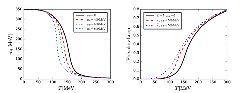
Figure 7: Left panel: $N_{f}=2+1$ constituent mass $\bar{m}_{l}$ of light quarks as a function of temperature $T$ at various baryon chemical potentials $\mu_{B}$.
Right panel: Polyakov loops $L$, $\bar{L}$ as functions of temperature $T$ at different baryon chemical potentials $\mu_{B}$.

V Results and discussion

In this section we discuss a selection of numerical results obtained in the present setup. We concentrate on $N_{f}=2+1$ flavour QCD, and use the corresponding results for $N_{f}=2$ only for the comparison of the $N_{f}=2$ and $N_{f}=2+1$ flavour QCD phase structures. Confinement and chiral symmetry breaking is discussed in Section V.1. Indications for an inhomogeneous phase at large chemical potential are shown in Section V.2. The strong couplings and propagators at finite $T$ and $\mu_{B}$ are discussed Section V.3. In Section V.4 we present phase structure of $N_{f}=2$ and $N_{f}=2+1$ flavour QCD at finite temperature and density.

In practice, we numerically solve the coupled set of flow equations discussed in the previous section together with the initial conditions discussed in Appendix E. As it has been discussed extensively in the literature, e.g.  Gies and Wetterich (2004); Braun and Gies (2007, 2010); Braun et al. (2011b); Mitter et al. (2015); Braun et al. (2016a); Pawlowski (2014); Rennecke (2015a); Cyrol et al. (2018a), the running couplings in the bound state sector are governed by an IR attractive fixed point in the chirally symmetric regime. As a consequence, if we initialise the flow in the perturbative regime, the initial conditions are fixed by the initial values of the strong coupling and the quark masses. As long as the initial meson masses are larger than the cutoff scale, our results are independent of the choice for the initial values in the meson sector, i.e. independent of any low-energy effective parameters. The low-energy sector emerges dynamically in our case, and the corresponding parameters cannot be tuned, but are predicted.

Note that the mutual coupling of the different $n$-point functions through their respective flow equations leads to a resummation of infinitely many diagrams upon integration of these equations. The renormalisation and regularisation provided by the fRG gives us access to the nonperturbative IR regime of QCD.

V.1 Chiral and confinement-deconfinement order parameters & signatures for the CEP

Observables and order parameters are derived from fields with nonvanishing expectation values: The scalar condensates $\bar{\sigma}_{\textrm{EoM}}$ and $\bar{\sigma}_{s,\textrm{EoM}}$ are directly related to dynamical chiral symmetry breaking, and the Polyakov loop and its conjugate, $L,\bar{L}$, are related to confinement, as introduced in Section III.6. Note however that these order parameters are not observables themselves.

In particular, the mesonic fields $\phi=(\sigma,\bm{\pi})$ are introduced as low energy effective fields that carry the dynamics of the scalar-pseudoscalar four-quark interaction. They carry the same quantum numbers as the related mesons but their direct physics interpretation in terms of onshell mesons has to be taken with a grain of salt. Nonetheless, the renormalised light chiral condensate and the reduced chiral condensate, $\Delta_{l,R}$ and $\Delta_{l,s}$ respectively, are given in terms of the unrenormalised expectation values $\sigma_{\textrm{EoM}}$ and $\sigma_{s,\textrm{EoM}}$, for more details see Appendix A. In the present work we concentrate on the renormalised light chiral condensate $\Delta_{l,R}$,

$$\Delta_{l,R}(T,\mu_{q})=-\frac{c_{\sigma}}{{2\cal N}_{R}}\left[\sigma_{\textrm{EoM}}(T,\mu_{q})-\sigma_{\textrm{EoM}}(0,0)\right]\,,$$ (118)

with a normalisation $-c_{\sigma}/(2{\cal N}_{R})$ which is fixed to the lattice, see also (133). The reduced condensate is also discussed in Appendix A, but carries a larger systematic error in the present approximation.

In turn, the Polyakov loop is an order parameter for confinement in pure Yang-Mills theory, but does not carry a direct physics interpretation in QCD with dynamical quarks. Despite these deficiencies both, $\bar{\sigma}_{\textrm{EoM}}$ and $(L,\bar{L})_{\textrm{EoM}}$ play a distinguished r$\hat{\textrm{o}}$le for the low energy dynamics of QCD.

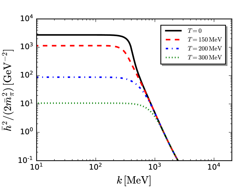
Figure 8: $N_{f}=2+1$ effective four-quark coupling $\bar{h}^{2}/(2\bar{m}_{\pi}^{2})$ in the pseudoscalar channel as a function of the RG scale $k$ at different temperatures and $\mu_{B}=0$.

In Figure 7 we show the constituent mass of light quarks and the Polyakov loop as functions of the temperature for several values of $\mu_{B}$. The size of the quark mass entails the strength of dynamical chiral symmetry breaking triggered by the scalar-pseudoscalar four-quark interaction. We see that both transitions are crossovers for small baryon chemical potential as is well-known due to explicit chiral and center symmetry breaking, see e.g. Aoki et al. (2006). They are getting sharper and shift to smaller temperatures with increasing $\mu_{B}$. As $L$ and $\bar{L}$ are related to the free energy of a single quark and antiquark respectively, they are different at finite $\mu_{B}$: Heuristically speaking, it is easier for an antiquark to propagate in a system with an excess of quarks, and hence $\bar{L}$ is larger than $L$ at finite, positive $\mu_{B}$.

As discussed in particular in Section III.5, the four-quark interaction plays a central r$\hat{\textrm{o}}$le for chiral symmetry breaking. The physical picture is that, as the strong coupling increases in strength with decreasing energy scale, the scattering of quark-antiquark pairs, mediated by gluon exchange, becomes stronger and eventually resonant. If this resonance occurs in the channel which carries the quantum numbers of a scalar quark condensate, $\langle\bar{q}q\rangle$, chiral symmetry is spontaneously broken. Dynamical hadronisation allows us to accurately capture the dynamics of the resonant quark-antiquark scattering channels in both the symmetric and the spontaneously broken phase. As argued in Section IV.3, the resulting effective four-quark interaction of the scalar-pseudoscalar channel is the given by the ratio $\bar{h}^{2}/(2\bar{m}_{\pi}^{2})$. In Figure 8 we show it as a function of the RG scale $k$ for several values of the temperature. Starting from large $k$, the coupling rises as expected from the increasingly strong quark-antiquark scattering. At $T=0$ and around $k\approx 400$ MeV, the increasingly steep rise indicates the resonance. The coupling turns into a pion-exchange interaction below this scale through dynamical hadronisation. Since the pion mass and the pion-quark Yukawa coupling are essentially constant in the chirally broken phase (cf. Figures 11 and 16), this interaction becomes approximately constant as well. The thermal suppression of the strong coupling discussed below leads to a suppression of the four-quark interaction with increasing temperature. As a consequence, the resonance disappears and chiral symmetry is restored at sufficiently high temperature. This is discussed in more detail in Braun and Gies (2006).

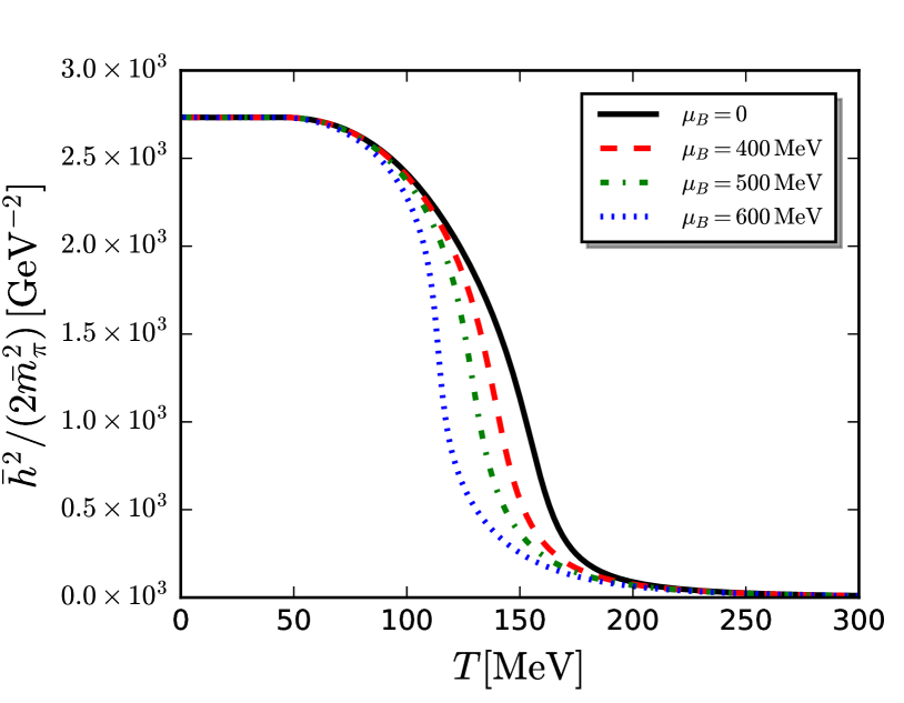
Figure 9: $N_{f}=2+1$ effective four-quark coupling $\bar{h}^{2}/(2\bar{m}_{\pi}^{2})$ at vanishing cutoff scale, $k=0$, in the pseudoscalar channel as a function of temperature $T$ at various baryon chemical potentials $\mu_{B}$.

In Figure 9 we show the effective four-quark interaction $\bar{h}^{2}/(2\bar{m}_{\pi}^{2})$ as a function of $T$ for $k=0$ for various chemical potentials. The insensitivity to $\mu_{B}$ at vanishing temperature is a consequence of the Silver Blaze property discussed in Section IV.1.1. For correlation functions below onset density, it implies that their dependence on $\mu_{B}$ is given solely by a $\mu_{B}$-dependent shift of the frequencies of external legs that carry baryon number. This is discussed in detail in Khan et al. (2015). For the present case, see Appendix J. For increasing temperature, the four-quark interaction melts down earlier and more rapidly with increasing $\mu_{B}$. Consequently, the chiral transitions occurs also more rapidly and at lower temperatures.

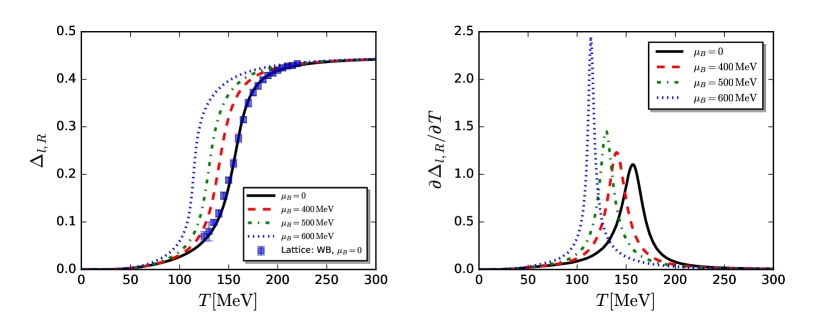
Figure 10: Left panel: $N_{f}=2+1$ renormalised light chiral condensate, $\Delta_{l,R}$, see Eqs. (133), (137), as a function of temperature $T$ at various baryon chemical potentials $\mu_{B}$. The normalisation constant in (133), (137) is chosen to match the scale in the lattice calculation Borsanyi et al. (2010).
Right panel: Thermal susceptibility of $N_{f}=2+1$ renormalised light chiral condensate, $\partial_{t}\Delta_{l,R}$, as a function of temperature $T$ at various baryon chemical potentials $\mu_{B}$.

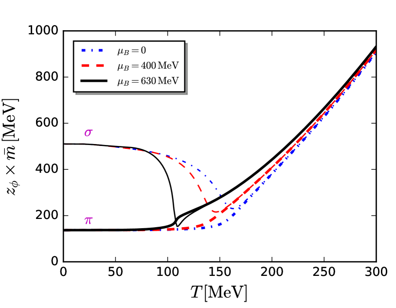
Figure 11: $N_{f}=2+1$ meson masses $\bar{m}_{\pi}$, $\bar{m}_{\sigma}$ as function of the temperature at different baryon chemical potentials $\mu_{B}$. They are rescaled by the multiplicative constant $z_{\phi}\equiv(\bar{Z}_{\phi}/Z_{\phi}(0))^{1/2}_{T,\mu_{B}=0}$. As a result, $z_{\phi}\,\bar{m}$ coincides with the pole mass defined in (88) and (98) in the vacuum. The in-medium behavior is that of the curvature masses defined in (43). For more details see Section IV.1.1.

The order parameter for chiral symmetry breaking used in the present work is the renormalised light chiral condensate $\Delta_{l,R}$, see Appendix A, in particular (137) and Figure 22. In Figure 10 (left panel) we show $\Delta_{l,R}$ as a function of temperature at various baryon chemical potentials. At $\mu_{B}=0$ we compare our result to the continuum extrapolation of lattice results at the physical point from Borsanyi et al. (2010) and find very good agreement. The corresponding thermal susceptibility, $\partial\Delta_{l,R}/\partial T$, is shown in the right plot of Figure 10. We use the peak position to define the pseudocritical temperature. We note that the pseudocritical temperature $T_{c}=156$ MeV at $\mu_{B}=0$ is in quantitative agreement with the lattice prediction. Similarly, one can use the inflection points of $\bar{m}_{l}$ and the Polyakov loop in Figure 7 to extract $T_{c}$, which yield 155 MeV and 153 MeV respectively, at vanishing baryon chemical potential. While these are not unique definitions of the crossover temperature, they match well with each other. For a more detailed comparison of chiral order parameters in the crossover regime see e.g. Pawlowski and Rennecke (2014).

The dynamics of the system at different $T$ and $\mu_{B}$ are reflected in the meson masses. They are shown in Figure 11. The splitting of the pion and $\sigma$ meson mass due to the chiral condensate is clearly visible. Furthermore, since $\bar{m}_{\sigma}$ is directly related to the inverse correlation length of the system, it has a dip at the chiral crossover. The closer the system is to the CEP, the lighter the sigma becomes at the transition until it eventually dips below $\bar{m}_{\pi}$. This indicates that the system enters the critical region, as visible in Figure 11 for $\mu_{B}=630$ MeV. At the CEP, the sigma is exactly massless since it is the critical mode of the chiral phase transition.

We also find that in the chirally symmetric phase $m_{\pi}$ and $m_{\sigma}$ become degenerate and grow rapidly with the increase of $T$. This entails that the mesonic degrees of freedom decouple quickly when the temperature of the system is above $T_{c}$. In this regime the dynamics are governed by the fundamental degrees of freedom of QCD. This will be discussed in more detail below. We note that the inclusion of only the resonant scalar-pseudoscalar interaction channel in the two-flavour subspace of 2+1 flavours entails that $U(1)_{A}$ is maximally broken. Hence, the mesons in the light sector that receive a positive contribution to their mass from the axial anomaly, $\eta^{\prime}$ and $\bm{a}_{0}$, are fully decoupled here. We defer a more complete study of chiral symmetry restoration, including the anomalous effects, to future work.

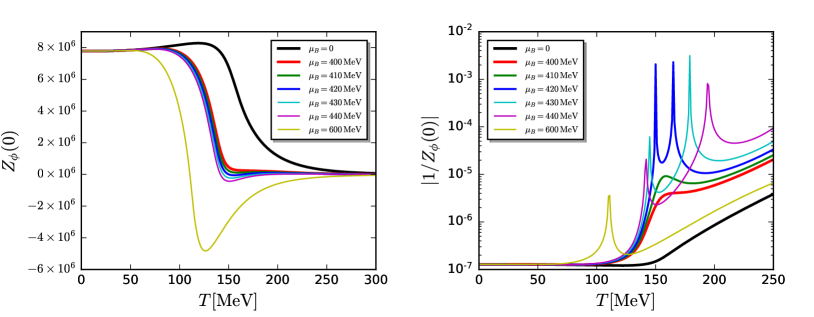
Figure 12: Left panel: $Z_{\phi}(0)$ at vanishing cutoff scale as a function of the temperature $T$ for various baryon chemical potentials $\mu_{B}$. Negative $Z_{\phi}(0)$, see (90), entails a negative spatial momentum slope of the dispersion $\Gamma^{(2)}_{\phi\phi}(p)$ at vanishing momentum. This indicates a minimum of the dispersion at a finite $\bm{p}^{2}\neq 0$.
Right panel: $\big{|}1/Z_{\phi}(0)\big{|}$ for the data in the left panel. Between the spikes the wave function renormalisation is negative at $\bm{p}^{2}=0$.

V.2 Inhomogeneous regime at large chemical potential

At finite chemical potential the situation changes significantly: The mesonic dispersion develops a minimum at nonvanishing momentum. This is signaled by $Z_{\phi}(0)$ at $k=0$ as defined in (85) and (90) turning negative. Indeed this happens for baryon chemical potentials $\mu_{B}\gtrsim 420$  MeV for a temperature regime that widens with increasing chemical potential, see Figure 12. The left panel shows $Z_{\phi}(0)$ as a function of temperature for different baryon chemical potentials, while the right panel shows $1/|Z_{\phi}(0)|$, which highlights the negative regime bounded by the spikes. This property entails that the mesonic two-point function develops a negative slope at vanishing momentum implying a minimum at nonvanishing spatial momentum, $\bm{p}^{2}_{\textrm{min}}\neq 0$. This signals a spatially modulated or inhomogeneous regime. Vanishing of the wave function renormalisation, as the coefficient of $\bm{p}^{2}$ in the meson propagator, can be indicative of an instability towards the formation of an inhomogeneous quark bound state, such as a chiral density wave. Whether or not inhomogeneous condensation occurs cannot be answered on the basis of only the meson wave function renormalisation. Such an analysis requires a systematic study of the competing effects of potential homogeneous and inhomogeneous resonances in quark-antiquark scattering channels. This will be deferred to future work. The relation between a minimum of the dispersion relation of bound states and inhomogeneous phases has been discussed in detail in the past decade within low energy effective theories at and beyond mean field. For reviews see e.g. Buballa and Carignano (2015); Anglani et al. (2014); Thies (2006); Schon and Thies (2000); Pisarski et al. (2019a), for applications with the functional RG see e.g. Carignano et al. (2014); Braun et al. (2016b); Roscher et al. (2015); Tripolt et al. (2018a).

This regime is indicated in the phase diagram in Figure 21. The blue shaded area corresponds to the region with $Z_{\phi}(0)<0$. The hatched red area denotes where this region overlaps with a sizable homogeneous chiral condensate. Note that the chiral phase boundary lies within this regime for baryon chemical potentials $\mu_{B}\gtrsim 500$  MeV. Hence, in particular in the hatched red region a competition between homogeneous and inhomogeneous quark-antiquark pairing is expected. This competing order effect can alter the phase structure. The hatched red region should therefore also be interpreted as a systematic error on our phase boundary. Accordingly, the present approximation should be upgraded by inhomogeneous four-quark interactions at larger $\mu_{B}$. Most notably, the CEP lies in this regime.

The connection between the CEP and inhomogeneous phases has been investigated within low energy effective theories, e.g. Carignano et al. (2014). It has been shown that the relative position of the onset of the inhomogeneous regime and the chiral CEP is related to the $\sigma$ mass gap, $m_{\sigma}$, and the constituent light quark mass, $m_{l}$. For $m_{l}=m_{\sigma}/2$ the two onsets agree on the mean field level. In this case the phases with restored chiral symmetry, the homogeneous phase and the inhomogeneous phase meet at a singe point, the Lifshitz point. For $m_{l}\geq m_{\sigma}/2$ the location of the (potential) chiral CEP is at larger baryon chemical potential as that for the onset of the inhomogeneous regime. In the present case we have $m_{l}\geq m_{\sigma}/2$ with $m_{l}/m_{\sigma}=347/510\approx 0.68$ in the vacuum. However, it has been argued in Pisarski et al. (2019b) that strong IR fluctuations wipe out the Lifshitz point. This could even lead to the destruction of the CEP. We emphasise that a detailed investigation of this regime goes beyond the scope of the present work but will be discussed in a forthcoming publication. However, we emphasise again that our observation of a minimum at nonzero spatial momentum in the mesonic dispersion is a strong indication for very interesting physics in this regime.

V.3 Dynamics and sequential decoupling

The relevance of the different fields for the dynamics of the system at different energy scales is encoded in the strength of the vertices and the propagator dressings. For example, we have already seen, that the effective four quark coupling $\bar{h}^{2}/(2\bar{m}^{2}_{\pi})$ decays rapidly for large momentum or cutoff scales, see Figure 8 and Figure 9. Accordingly, the quark-self coupling gets irrelevant in the UV. Moreover, for increasing temperature and chemical potential the effective four quark coupling decreases further. In the present parameterisation with dynamical hadronisation this decoupling is solely triggered by the increase of the pion mass function $\bar{m}^{2}_{\pi}$, for the temperature dependence of the mesonic mass functions see Figure 11. In turn, the Yukawa interaction does not show a significant momentum scale and parameter dependence, see Figure 16 and discussion there. Similar observation apply to the gluonic sector. All avatars of the strong coupling show a rather strong scale dependence, as do the gluon and meson dressings. This will be discussed in the following. In combination, the different dynamics and scale dependence of the couplings, wave function renormalisations and mass functions allow us to provide a consistent picture of a sequential decoupling of gluon, quark and mesonic degrees of freedom with decreasing momentum and cutoff scales. This leads to the natural emergence of low energy effective theories (LEFTs) of QCD for scales below $\sim 1$  GeV and is discussed at the end of the present Section.

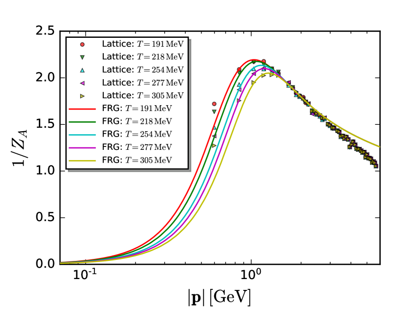
Figure 13: $N_{f}\!=\!2\!+\!1$ gluon dressing function $1/Z_{A}$ as a function of spatial momenta $|{\bm{p}}|$ at different temperatures in comparison to the $N_{f}\!=\!2\!+\!1\!+\!1$ lattice data from Ilgenfritz et al. (2018), based on the tmfT configurations Burger et al. (2013), for the tmfT simulation setup see also Baron et al. (2010a, b). The lattice results depicted here are obtained for $\beta=2.1$, $a=0.0646\,$fm and an approximate pion mass of $m_{\pi}=369(15)$ MeV leading to a pseudocritical temperature of $T_{\textrm{deconf}}=193(13)(2)$ MeV, for more details see Ilgenfritz et al. (2018).

We start our analysis of the dynamics and decoupling properties of the system with the gluon dressing. Here we also provide a further benchmark test of the present approach at vanishing baryon chemical potential: In Figure 13 we compare our results at finite $T$ and $\mu_{B}=0$ to lattice results on the magnetic gluon dressing function from Ilgenfritz et al. (2018) based on the tmfT configurations Burger et al. (2013); for this simulation setup see also Baron et al. (2010a, b). Note that the lattice results are obtained for $N_{f}\!=\!2\!+\!1\!+\!1$ flavours, with $\beta=2.1$, $a=0.0646\,$fm and an approximate pion mass of $m_{\pi}=369(15)$ MeV leading to a critical temperature of $T_{\textrm{deconf}}=193(13)(2)$ MeV. Hence, agreement with our results can only be expected at large temperatures and the corresponding spatial momentum scales. In this regime, the vacuum constituent quark masses are small against their thermal masses and the perturbative running of $N_{f}=3$ vs $N_{f}=4$ is not yet dominant. Furthermore, the effects of the additional quark flavour and the different masses are subleading. In order to facilitate this comparison, we rescaled our momentum scale by $|\bm{p}|\rightarrow 1.07|\bm{p}|$ as to match our results in the semiperturbative regime around $p\approx 2$ GeV. This is necessary since, owing to the different mass scales, also the momentum scales of our results and the lattice results are inherently different. Indeed, we find good agreement for the temperatures, 191, 218, 254, 277 and 305 MeV, for $0.8\,\textrm{GeV}\lesssim|\bm{p}|\lesssim 3$​ GeV. For larger momenta, our result show the correct leveling-off expected from the logarithmic momentum dependence in the perturbative regime. For smaller momenta, both the different mass scales and the different infrared gauge fixing come into play. Note also that the lattice data are subject to lattice artefacts at large momenta, as is the case in the $N_{f}=2$ vacuum data, see Figure 25.

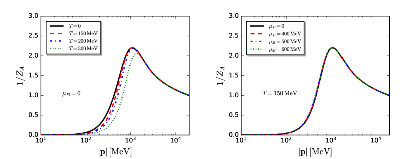
Figure 14: $N_{f}=2+1$ gluon dressing function $1/Z_{A}$ at vanishing Matsubara frequency, $p_{0}=0$, as a function of spatial momenta $|{\bm{p}}|$ at different temperatures (left panel) and baryon chemical potentials (right panel). As for the $N_{f}=2$ flavour input data and the $N_{f}=2+1$ vacuum results, see Figure 3, we use the identification $\bm{p}^{2}=k^{2}$.

In Figure 14 we show the gluon dressing function $1/Z_{A}(|\bm{p}|)=1/Z_{A,k=|\bm{p}|}$ at vanishing Matsubara frequency $p_{0}=0$ as a function of spatial momenta for different temperatures (left panel) and baryon chemical potentials (right panel). While the gluon dressing shows a mild dependence on the temperature, it is essentially independent on the baryon chemical potential. Note that the respective dependences are more significant in the gluon propagator $G_{A}=1/(p^{2}Z_{A}(p))$ shown in Figure 29 in Appendix H. However, we emphasise that the flows of the couplings and observables computed in the present work depend on the gluon dressing rather than on the gluon propagator.

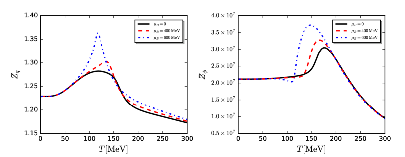
Figure 15: $N_{f}=2+1$ quark (left panel, $Z_{q}$) and meson (right panel, $\bar{Z}_{\phi}$) wave function renormalisations at vanishing cutoff scale, $k=0$, as functions of temperature $T$ at different baryon chemical potentials $\mu_{B}$.

The suppression of the thermal and chemical potential dependences discussed above are linked to the mass gap of the gluon propagator in the Landau gauge. This mass gap signals confinement, see Braun et al. (2010a); Marhauser and Pawlowski (2008); Braun et al. (2010b); Fister and Pawlowski (2013); Herbst et al. (2015), and manifests itself through the nonmonotonicity of the curves depicted in Figure 14. The backbending of the gluon propagator at small momenta also signals positivity violation Alkofer and von Smekal (2001), and results in a negative spectral function at low frequencies Cyrol et al. (2018c). With increasing temperature above $T_{c}$, the chromoelectric part of the gluon is subject to increasingly strong Debye-screening. As discussed in Section IV.1.2, we define the gluon dressing via the chromomagnetic contribution. Hence, the thermal suppression in the left plot of Figure 14 is due to nonperturbative magnetic screening. For more technical details on the in-medium gluon propagator we refer to Section IV.1.2 and Appendix H.

Overall, the temperature dependence of the gluon dressing is a subleading effect in the temperature region relevant for the phase transition. Below the critical temperature it is mostly affected in the infrared, where the mass gap suppresses gluon fluctuations anyway. While thermal corrections are also present in the pure gauge theory, density corrections are only triggered by the quark contributions discussed in Section IV.1.2. We find that the gluon dressing function is almost insensitive to $\mu_{B}$. This is shown in the right plot of Figure 14, and also in Figure 29 for the propagators itself. For temperatures in the vicinity of the crossover, we find a slight enhancement of the gluon propagator with increasing $\mu_{B}$ for momenta below $\sim 1$ GeV. The reason is that the quark contribution to the gluon propagator, i.e. the vacuum polarisation, is suppressed at finite $\mu_{B}$, which can be read-off from the explicit expression in (208). This counteracts the color screening of quarks. These findings support the qualitative or even semiquantitative approximations in functional applications (fRG and DSE), where either both or part of the thermal and density dependence of the gluon dressing is left out.

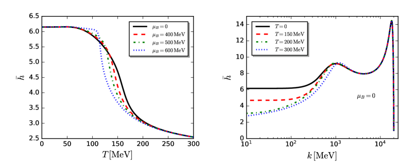
Figure 16: Left panel: $N_{f}=2+1$ Yukawa coupling at vanishing cutoff scale, $k=0$, as a function of the temperature $T$ at different baryon chemical potentials $\mu_{B}$.
Right panel: $N_{f}=2+1$ Yukawa coupling as a function of the RG scale $k$ at different temperatures $T$ and vanishing baryon chemical potential $\mu_{B}=0$.

The quark and meson wave function renormalisations and their dependence on $T$ and $\mu_{B}$ are shown in Figure 15. Owing to our choice of regulators, shown in (225a) and (225b), $Z_{q,k}$ and $Z_{\phi,k}$ enter the system of flow equations only indirectly through the corresponding anomalous dimensions, (30). Consequently, the flows of the wave function renormalisations do not have to be integrated and their initial values are irrelevant. We have chosen $Z_{k=\Lambda}=1$ for convenience, see (41). One observes that there is a bump in $Z_{q}$ as a function of $T$ during the phase transition, and it evolves into a sharp peak with the increase of the baryon chemical potential. This indicates that constituent quark fluctuations are enhanced in the vicinity of the phase transition at finite $\mu_{B}$. We also find that the meson wave function renormalisation decreases after chiral symmetry is restored. This effect drives the decoupling of mesons from the physical spectrum above $T_{c}$, which is also visible in Figure 11 and discussed in the previous section.

Interestingly, the renormalised Yukawa coupling, (43), is relatively stable over all scales. Accordingly, the quark-meson vertex running counterbalances the strong scale dependence of the meson wave function renormalisation. This is explicitly seen in Figure 16: On the left side we show the temperature and chemical potential dependence of the physical Yukawa coupling, $\bar{h}_{k=0}$. On the right side we show its running with $k$ at different temperatures. The Yukawa coupling is related to the expectation value of the renormalised $\bar{\sigma}$-field and the constituent mass of the light quarks via $\bar{h}_{k=0}=2\bar{m}_{q}/\langle\bar{\sigma}\rangle$. In the symmetric phase, the fast decrease of $\bar{h}$ with increasing $T$ triggers a more rapid melting of $\bar{m}_{q}$ as compared to $\langle\bar{\sigma}\rangle$. It is evident from the running of the Yukawa coupling in the right panel of Figure 16 that thermal corrections only set in if the RG scale is smaller than the temperature scale, $k\lesssim 2\pi T$. For larger $k$ and the 3d spatial regulators used here, see Appendix N, they are exponentially suppressed with $\exp(-k/(2\pi T))$ and there is only the vacuum running. For a respective discussion of the thermal properties including also other regulators we refer to Fister and Pawlowski (2015). Furthermore, we have explicitly checked that our results are independent of the initial value of the Yukawa coupling: The Yukawa coupling is an irrelevant coupling that is generated by the flow. The memory of its initial condition is washed-out by an IR-attractive fixed point in the regime of small strong coupling. This is in line with the discussion at the beginning of this section.

This stability of the renormalised Yukawa coupling together with the rapid rise of the meson mass parameters $\bar{m}_{\sigma},\bar{m}_{\pi}$ entails the decoupling of the scalar-pseudoscalar mesonic channel of the four-quark interaction in the chirally symmetric phase at large scales, discussed in Section V.1.

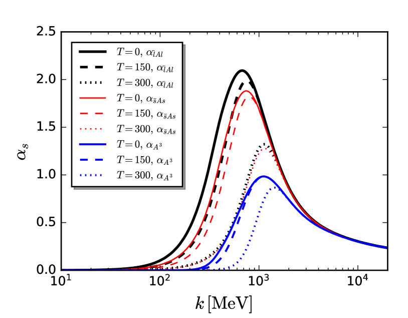
Figure 17: $N_{f}=2+1$ quark-gluon coupling for light quarks ($\alpha_{\bar{l}Al}$) and strange quarks ($\alpha_{\bar{s}As}$) quarks, and three-gluon coupling ($\alpha_{A^{3}}$) as functions of the RG scale $k$ for several values of the temperature $T$ and for vanishing baryon chemical potential, $\mu_{B}=0$.

For larger scales, $k\gtrsim 1$ GeV, the gluon exchange interactions are dominating the system, while for smaller scales, $k\lesssim 1$ GeV, the gluons decouple. This is clearly seen in Figure 17, where we show the running of the different strong couplings: The quark-gluon and the three-gluon couplings. We have distinguish between the quark-gluon coupling for $u$ and $d$ quarks, denoted by $\alpha_{\bar{l}Al}$, and for the $s$ quark, $\alpha_{\bar{s}As}$. The quark-gluon couplings $\alpha_{\bar{l}Al}$ and $\alpha_{\bar{s}As}$ match for momentum scales $k$ above $\sim 1$ GeV. In turn, the strange quark coupling is slightly smaller at lower scales. This is expected since quark number conservation of the strong interactions implies that there is no flavour mixing in the quark-gluon interactions. Hence, only strange quarks contribute to the leading quantum corrections of $\alpha_{\bar{s}As}$, resulting in a suppression relative to the leading corrections to $\alpha_{\bar{l}Al}$.

The quark-gluon couplings and the three-gluon coupling agree with each other, and are also consistent with perturbation theory, for scales above $\sim 5$ GeV Braun et al. (2016a); Cyrol et al. (2018a). One also finds that for scales $k\lesssim 5$  GeV, the light flavour coupling $\alpha_{\bar{l}Al}$ and the strange coupling $\alpha_{\bar{s}As}$ grows bigger than $\alpha_{A^{3}}$, which is qualitatively consistent with the calculation in Cyrol et al. (2018a). For scales $k\lesssim 1-2$ GeV, $\alpha_{\bar{l}Al}$, $\alpha_{\bar{s}As}$ and $\alpha_{A^{3}}$ deviate from each other pronouncedly, and all strong couplings are suppressed significantly. This behavior in the IR region is due to the running of the gluon dressing function shown in the left panel of Figure 14 and our definition of the strong couplings in (54) and (55). Since they effectively describe gluon exchange, the suppression of glue dynamics in the nonperturbative regime due to the dynamically generated gluon mass gap is transferred to the RG invariant strong couplings. Apparently, the three-gluon coupling is more suppressed than the quark-gluon vertex in the IR, since more gluons are attached to the former, which is verified in Figure 17. The dependence of the strong couplings on the temperature is consistent with our expectation inferred from the results of the gluon propagator. The strong couplings decrease with the increase of the temperature, which indicates the interaction between gluons and quarks gets weaker at high temperature. We have also investigated the dependence of the strong couplings on the baryon chemical potential, and find a small $\mu_{B}$- dependence in the $\mu_{B}$ region of our interest.

We close this Section with a discussion of sequential decoupling and the natural emergence of low energy effective theories (LEFT) in the present fRG approach to QCD for low cutoff scales $k\lesssim 1$ GeV: The flows of matter vertices and propagators (quarks and mesons) are driven by the tree-level four-point single field exchange couplings with either quark or meson legs in the current approach. We emphasise that this is not due to the approximations used here but originates in the one loop completeness of the flow equation for the effective action, (26). Relevant examples are provided by the flows of the quark-gluon and Yukawa couplings depicted in Figure 6, and the flow of the four quark coupling depicted in Figure 4. These flows contain all single field exchange couplings considered in the present approach: The four-quark single gluon exchange coupling and the four-quark single meson exchange coupling. Note that the potential third single field exchange coupling, the two-quark–two-meson single quark exchange coupling simply comes from a reordering of the building blocks in the diagrams. It also originates in the fundamental building blocks in the QCD matter sector considered here, the scalar-pseudoscalar channel of the four-quark interaction. Accordingly, the two-quark–two-meson single quark exchange coupling simply measures the strength of the Yukawa coupling and has no physical interpretation. In particular, it does not entail a possible decoupling. This leaves us with

$$g^{2}_{\bar{q}Aq}\,,\qquad\qquad\frac{\bar{h}^{2}}{1+\tilde{m}_{\phi}^{2}}\,,$$ (119)

with $\phi=\sigma,\bm{\pi}$ and the dimensionless mass functions $\tilde{m}$ defined in (197). Note also that these exchange couplings generate genuine four-field interactions in the flow, such as the four-quark and four-meson vertices. Consequently, the strength of these higher order couplings is tightly linked to that of the single field exchange couplings, the analysis of which suffices in the absense of additional resonant interaction channels besides the scalar-pseudoscalar one.

In Figure 18 we depicted the two fundamental single field exchange couplings defined in (119). The UV dominance of the gluonic exchange coupling for cutoff scales $k\gtrsim 1$ GeV is clearly visible. In turn, for cutoff scales $k\lesssim 1$ GeV the mesonic exchange coupling takes over gradually with $g_{\bar{l}Al}^{2}=\bar{h}^{2}/(1+m_{\pi}^{2})$ at $k\approx 600$  MeV, while the gluonic coupling decays more quickly. Note that the exchange couplings only provide the qualitative picture; the respective flow diagram also have different combinatorial factors from the different colour and flavour traces. For the four-quark flow a details comparison is done in Appendix L, and is summarised in Figure 30.

In the matter-dominated regime the best indicator for the further decoupling is given by the respective propagator gapping

$$\frac{1}{1+\tilde{m}_{q}^{2}}\,,\qquad\frac{1}{1+\tilde{m}_{\phi}^{2}}\,,$$ (120)

with $\phi=\sigma,\bm{\pi}$, $q=l,s$ and the $\tilde{m}$ defined in (197). These gapping functions are depicted in Figure 19, where also the full gluon dressing is displayed for the sake of comparison. Note that the latter does not only entail the gapping information for cutoff scales smaller than that of the peak postion of the dressing function, $k\lesssim k_{\textrm{peak}}$, but also the running of the gluon wave function for $k\gtrsim k_{\textrm{peak}}$. Qualitatively, this carries the same information as that depicted in Figure 18: gluonic fluctuations decouple first. However, Figure 18 carries the full decoupling which also requires the coupling strengths of quark-gluon vertex and Yukawa vertex respectively.

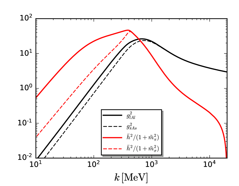
Figure 18: Dimensionless four-quark single gluon exchange coupling ($g^{2}_{\bar{l}Al}$ and $g^{2}_{\bar{s}As}$) and four-quark single meson exchange couplings ($\bar{h}^{2}/(1+\tilde{m}_{\pi}^{2})$ and $\bar{h}^{2}/(1+\tilde{m}_{\sigma}^{2})$) as functions of the cutoff scale $k$ in the vacuum. Gluons, quarks, and mesons decouple sequentially from the matter dynamics.

In turn, after the decoupling of the gluonic sector the interactions between quark and mesons only depend on the Yukawa coupling, and the respective propagator gapping is sufficient for the decoupling information: the propagator gappings of quarks and mesons clearly entail that diagrams with quark propagators decouple first (first strange, than the light quark diagrams). The $\sigma$-field decouples at roughly the same scale as the light quarks and finally the contributions of pion diagrams tend towards zero below the pion mass scale.

In summary, the sequential decoupling is clearly seen. First the gluonic dynamics decouples from the matter sector, then the quark and $\sigma$ exchange diagrams decouple and finally the pion decouples. For example, this already entails that in the vacuum chiral perturbation theory emerges naturally in this setup, for investigations of respective low energy parameters see e.g. Divotgey et al. (2019); Eser et al. (2019). Moreover, it allows us to also investigate the validity bounds of chiral perturbation theory. Note also that the ordering in the sequential decoupling is changes at finite density. In particular the $\sigma$ mode decouples later in the vicinity of the CEP, where, as the critical mode, gets massless.

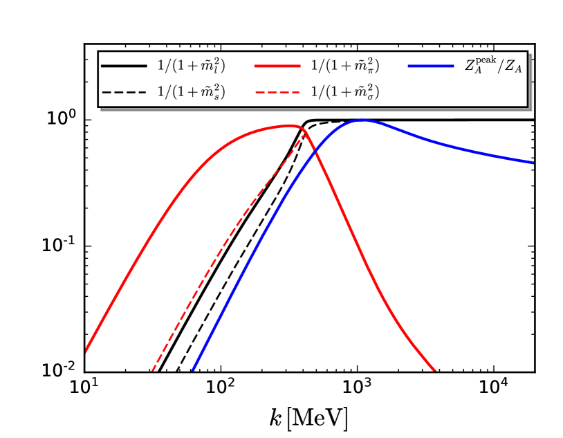
Figure 19: Dimensionless propagator gapping $1/(1+\tilde{m}^{2}_{\Phi_{i}})$ for $\Phi_{i}=l,s,\sigma,{\bm{\pi}}$. For comparison, we also show the gluon dressing function $Z_{A}^{\textrm{peak}}/Z_{A}$ with the solid blue line. Here, $1/Z_{A}$ is normalised by its peak position at $k_{\textrm{peak}}$, that is $Z_{A}^{\textrm{peak}}=Z_{A}(k_{\textrm{peak}})$: for cutoff scales $k\gtrsim k_{\textrm{peak}}$ the $k$-dependence of $Z_{A}$ is dominated by the running of the gluon wave function renormalisation, for $k\lesssim k_{\textrm{peak}}$ it shows the gluon gapping. In summary, the sequential decoupling of gluon, quark and meson dynamics towards the IR is evident here.

This leads us to an intriguing and simple picture: Initiating the QCD flow at a large perturbative cutoff scale $k=\Lambda^{\textrm{UV}}_{\textrm{QCD}}$, here $\Lambda^{\textrm{UV}}_{\textrm{QCD}}=20$ GeV, the flow towards smaller scales leaves us with the dynamics of quarks and mesons for $k\ll 1$  GeV. In the present setup with dynamical hadronisation we flow into a Polyakov loop enhanced quark meson model. In turn, without dynamical hadronisation we arrive at a Polyakov loop enhanced NJL-type model. We also emphasise that while the offshell dynamics of gluons decouples, the gluon sector still leaves its imprint in terms of the quantum equations of motion for the gluonic background $A_{0}$ or $L,\bar{L}$.

Hence, the underlying assumption of LEFTs, that high-energy degrees of freedom are integrated out, can be made explicit with the present setup. Moreover, this can also provide valuable reliability checks for LEFTs. In summary this provides an explanation and further reliability. The sequential decoupling demonstrated here adds further justification for the unreasonable effectiveness of LEFTs in QCD. For a selection of fRG work on QCD LEFTs see Schaefer and Wambach (2005, 2007); Herbst et al. (2011); Skokov et al. (2010, 2011); Braun et al. (2012); Strodthoff et al. (2012); Fukushima and Pawlowski (2012); Aoki and Sato (2013); Kamikado et al. (2013); Jiang and Zhuang (2012); Haas et al. (2013); Herbst et al. (2014, 2013); Tripolt et al. (2014); Grahl and Rischke (2013); Mitter and Schaefer (2014); Herbst et al. (2014); Morita et al. (2013); Pawlowski and Rennecke (2014); Helmboldt et al. (2015); Braun et al. (2016c); Khan et al. (2015); Wang and Zhuang (2016); Mueller and Pawlowski (2015); Eser et al. (2015); Weyrich et al. (2015); Fu and Pawlowski (2015); Aoki et al. (2016); Fejos (2015); Jiang et al. (2016); Fu and Pawlowski (2016); Fu et al. (2016); Rennecke and Schaefer (2017); Jung et al. (2017); Fejos and Hosaka (2016); Almasi et al. (2017a); Posfay et al. (2018); Yokota et al. (2016); Springer et al. (2017); Resch et al. (2019); Tripolt et al. (2018a); Braun et al. (2017); Fejos and Hosaka (2017); Yokota et al. (2017); Almasi et al. (2017b); Zhang et al. (2017); Aoki et al. (2018); Braun et al. (2018); Fejos and Hosaka (2018); Braun et al. (2019a); Fu et al. (2018a, b); Sun et al. (2018); Wen et al. (2019); Yin et al. (2019); Leonhardt et al. (2019); Li et al. (2019a).

We emphasise that the emergence of QCD LEFTs in the infrared at scales $k\lesssim 1$ GeV within the current approach allows for their systematic improvement in terms of QCD-assisted LEFTs, and constitutes important progress in the setup and the qualitative and quantitative reliability of low energy effective theories. Of course, QCD LEFTs in general rely on QCD information. For example, the parameters of QCD LEFTs used for QCD at finite temperature and density are typically fixed with vacuum observables such as the pion decay constant and meson masses as well as quark constituent masses. Further QCD input ranges from the enhancement of the models with a Polyakov loop potential that carries information about the confinement-deconfinement phase transition.

A step in the direction towards using dynamical or fluctuation information of QCD is done with the implementation of the QCD-running of external parameters such as the critical temperature parameter $T_{0}$ in the Polyakov loop potential as suggested in Schaefer et al. (2007). A first example for a QCD-assisted LEFTs is then provided by Haas et al. (2013); Herbst et al. (2014), where the phenomenological approach in Schaefer et al. (2007) was confirmed and improved by results for the Polyakov loop potential from fRG-computations in Yang-Mills theory Braun et al. (2010a); Fister and Pawlowski (2013) and $N_{f}=2$ flavour QCD Braun et al. (2011a). Another example is provided by Springer et al. (2017), where the UV initial conditions for the QCD LEFT were computed from QCD flows.

The results and in particular the flows of the current work can be readily used as external input for QCD LEFTs, hence lifting them to QCD-assisted LEFTs. An interesting and relevant example under progress is provided by fluctuation observables such as cumulants of net-particle multiplicity distributions, e.g. Fu et al. (2016, 2018b). A qualitative improvement of the computations there is given by utilising the quark-gluonic flows from the present work as external input. This provides quantitative reliability of the results at large density or small $\sqrt{s}$ relevant for the search of the critical end point.

V.4 Phase Structure of $N_{f}=2$ and $N_{f}=2+1$ flavour QCD

In Figure 20 we show our results on the phase structure in $T$-$\mu_{B}$ plane for $N_{f}=2$ and $N_{f}=2+1$ flavours. In both cases, as discussed in Section V.1, we define the pseudocritical temperature via the thermal susceptibility of the renormalised light chiral condensate, $\partial\Delta_{l,R}/\partial T$. At vanishing baryon chemical potential, the respective chiral transition temperatures are

$$T_{c,{\tiny{N_{f}=2}}}=171\,\textrm{MeV}\,,\qquad T_{c,{\tiny{N_{f}=2+1}}}=156\,\textrm{MeV}\,.$$ (121)

The width of the transition is taken to be the full width at 80% of the maximum of this susceptibility. For $N_{f}=2$, the crossover phase boundary is given by the long-dashed red line and its width by the gray band. The corresponding CEP is denoted by the red star. For $N_{f}=2+1$, the short-dashed black line marks the phase boundary and the blue band its width. The black point shows our result for the CEP of $N_{f}=2+1$ QCD.

At small chemical potential lattice results provide a benchmark test for the present fRG computations. This includes the curvature of the phase boundary. It is a sensitive measure for the correct relative strength of quantum, thermal and density fluctuations. The curvature coefficient $\kappa$ of the phase boundary at vanishing baryon chemical potential is the quadratic expansion coefficient of $T_{c}(\mu_{B})$ around $\mu_{B}=0$, i.e.,

$$\frac{T_{c}(\mu_{B})}{T_{c}} =1-\kappa\left(\frac{\mu_{B}}{T_{c}}\right)^{2}+\lambda\left(\frac{\mu_{B}}{T_{c}}\right)^{4}+\cdots\,,$$ (122)

with $T_{c}=T_{c}(\mu_{B}=0)$. We refer, e.g., to Fischer (2019) for additional relevant discussions. As for the transition temperature, the curvature of the phase boundary of a crossover depends on its definition Pawlowski and Rennecke (2014). By using the renormalised light chiral condensate, we ensure comparability with the lattice results in Bellwied et al. (2015); Bazavov et al. (2019). To extract the curvature, we fit our numerical results for $T_{c}(\mu_{B})/T_{c}$ by the polynomial given in (122) for orders 2 and 4 in $\mu_{B}/T_{c}$ within the regions $\mu_{B}/T\leq 2$ and 3, and read-off the corresponding quadratic coefficient $\kappa$. Our final result for the curvature with its numerical error is then given by the mean and the standard deviation of all these coefficients.

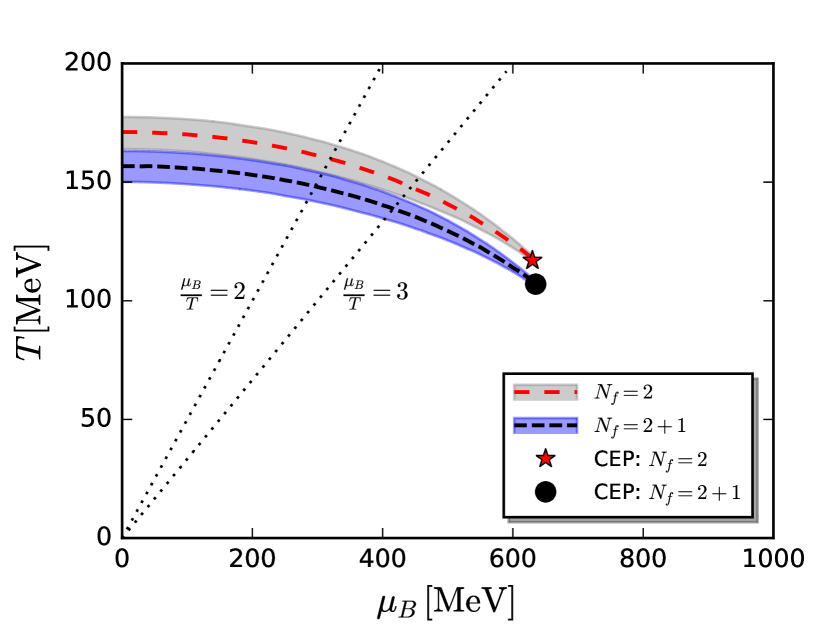
Figure 20: Phase diagram in the plane of the temperature and the baryon chemical potential. The gray and blue bands denote the crossover transitions for the $N_{f}=2$ and 2+1 flavour QCD, respectively; and the red star and black circle are their relevant CEP. The bands are determined through the 80$\%$ peak height of $\partial\Delta_{l,R}/\partial T$ at fixed $\mu_{B}$. The black and red dashed lines depict the peak positions for the $N_{f}=2+1$ and $N_{f}=2$, respectively. We also provide the two lines of $\mu_{B}/T=2,3$ related to reliability bounds for both lattice and functional methods.

The curvature for the two-flavour pseudocritical line is determined to be

$$\kappa_{{}_{\tiny{N_{f}=2}}}=0.0176(1)\,.$$ (123)

For the curvature of the 2+1 flavour phase boundary we find

$$\kappa_{{}_{\tiny{N_{f}=2+1}}}=0.0142(2)\,.$$ (124)

As has been emphasised before, our results are consistent with recent $N_{f}=2+1$ lattice results, e.g. $\kappa=0.0149(21)$ in Bellwied et al. (2015) and $\kappa=0.015(4)$ in Bazavov et al. (2019). Note also that $\kappa_{{}_{\tiny{N_{f}=2}}}\approx\kappa_{{}_{\tiny{N_{f}=2+1}}}(T_{c,{\tiny{N_{f}=2}}}/T_{c,{\tiny{N_{f}=2+1}}})^{2}=0.171$. This entails that the two dimensionless phase transition lines given by $T_{c}(\mu)/T_{c}(0)$ in (122) agree for small baryon chemical potentials. This even holds for a large $\mu_{B}$-range as can be already deduced from Figure 20.

All results, including DSE, are summarised in Table 2. For a comparison to other results and potential implications for experimental CEP searches, we also refer to the discussion in the introduction, Section I, and in particular Figure 1.

	$N_{f}=2$	$N_{f}=2+1$
fRG: this work	0.0176(1)	0.0142(2)
lattice: Bellwied et al. (2015)		0.0149(21)
lattice: Bonati et al. (2018)		0.0144(26)
lattice: Bazavov et al. (2019)		0.015(4)
DSE: Fischer et al. (2014a)		0.0238
DSE: Gao et al. (2016)		0.038
lattice: Allton et al. (2002)	0.0078(39)
lattice: de Forcrand and Philipsen (2002)	0.0056(6)

Table 2: Curvature coefficients $\kappa$, see (122): from the fRG: present work; Lattice collaborations: Bellwied et al. (2015) (WB), Bonati et al. (2018) (Bonati et al.), Bazavov et al. (2019) (hotQCD), Allton et al. (2002) (Allton et al.), de Forcrand and Philipsen (2002) (Forcrand and Philipsen), Lattice overviews Philipsen (2007); D’Elia (2019); DSE: Fischer et al. (2014a) (Fischer et al.), Gao et al. (2016) (Gao et al.), DSE overview Fischer (2019).

At finite baryon chemical potential lattice simulations are hampered by the sign problem, resulting in increasing statistical and systematic errors with increasing $\mu_{B}$. The former are shown in Figure 1, the latter are unknown. The respective validity bounds are indicated by the dashed lines at $\mu_{B}/T=2$ and $\mu_{B}/T=3$ in Figure 20. For $\mu_{B}/T$ close to the crossover line and larger than $\mu_{B}/T=3$ also the approximations used in the present work start to lose reliability: In the presence of the nontrivial mesonic dispersions, the phase structure can be altered, cf. Section V.2. Accordingly, results in this regime, including our result for the location of the CEP, have to be interpreted with care.

We find CEPs for $N_{f}=2$ and $N_{f}=2+1$ flavour QCD at

$$(T_{{}_{\tiny{\text{CEP}}}},{\mu_{B}}_{{}_{\tiny{\text{CEP}}}})_{{}_{\tiny{N_{f}=2}}}=(117,630)\,\textrm{MeV}\,,$$ (125)

and

$$(T_{{}_{\tiny{\text{CEP}}}},{\mu_{B}}_{{}_{\tiny{\text{CEP}}}})_{{}_{\tiny{N_{f}=2+1}}}=(107,635)\,\textrm{MeV}\,,$$ (126)

respectively. This amounts to rather large values of ${\mu_{B}}_{{}_{\tiny{\text{CEP}}}}/T_{{}_{\tiny{\text{CEP}}}}$ of

$$N_{f}=2: \ \frac{{\mu_{B}}_{{}_{\tiny{\text{CEP}}}}}{T_{{}_{\tiny{\text{CEP}}}}}=5.38\,,$$

$$N_{f}=2+1: \ \frac{{\mu_{B}}_{{}_{\tiny{\text{CEP}}}}}{T_{{}_{\tiny{\text{CEP}}}}}=5.93\,.$$ (127)

Our results for the CEP are extracted from the onset of critical scaling on the chiral phase boundary. As discussed in Section IV.4 and Appendix F, we expand the effective potential about its running minimum. The flow of the minimum is proportional to the correlation length $1/\partial_{\bar{\sigma}}^{2}\bar{V}_{k}\big{|}_{\textrm{EoM}}$ (cf. (159b)), and hence becomes unstable in the critical region. We use this instability to determine where the system enters the critical region from below in $\mu_{B}$. To pin down the location of the CEP, we exploit the well established fact that, owing to the very small pion mass and strong mesonic fluctuations close to the CEP, the critical region is at most a few MeV wide in $\mu_{B}$; see e.g. Herbst et al. (2011). We emphasise that the critical properties are solely driven by the quark-meson fluctuations and hence QCD LEFT investigations are fully applicable here. Accordingly, to very high accuracy, the CEP is located at the point on the phase boundary where the running minimum becomes unstable.

We emphasise that the reduced reliability of our results at large $\mu_{B}$ is not of conceptual origin, as opposed to the sign problem on the lattice. It is related to correlation functions that have been neglected in our truncation of the effective action. Improvements require the systematic inclusion of additional momentum-dependences of correlation functions. Moreover, a Fierz complete basis of the four-quark tensor structures should be taken into account, including potentially dynamical hadronisation of additional resonant channels. This is work in progress within the fQCD collaboration Braun et al. (2019c).

A physically intriguing source for part of the systematic error in the present work is related to the indications of an inhomogeneous regime we discussed in Section V.2. To highlight the potential effect on the phase boundary, we show the region where the meson wave function renormalisation at vanishing spatial momentum is negative, $Z_{\phi}(0)<0$, with the shaded blue area in Figure 21. Note that we only scanned the phase diagram for $\mu_{B}<{\mu_{B}}_{{}_{\tiny{\text{CEP}}}}$. Hence, the boundary of the shaded blue region at $\mu_{B}=635$ MeV is of no physical significance. As discussed in Section V.2, the possibility of inhomogeneous condensation leads to a competition between potential resonances in the homogeneous and inhomogeneous quark-antiquark interaction channels. Regarding the phase structure itself, this is most relevant when condensation occurs in the first place. The region where the mesonic dispersion with a minimum at nonvanishing spatial momentum overlaps with a sizable condensate, defined in Section V.2 and the caption of Figure 21, is given by the hatched red area in this figure. There, the phase structure could be altered significantly by possible inhomogeneities. To put his into perspective, we also added a selection of freeze-out points to Figure 21. It is very intriguing that the inhomogeneous regime could be probed in heavy-ion collisions at small beam energies of roughly $\sqrt{s}\lesssim 6$ GeV.

VI Critical end point and systematic error estimates in functional approaches

Here we combine the up-to-date CEP results of functional approaches for a first estimate of the most likely region of the CEP. To that end we discuss the respective approximations and the potential effect of missing fluctuations. A full discussion of the respective systematic errors is deferred to future work as it goes far beyond the scope of the present work.

The results for the phase structure in the present fRG approach are summarised in Figure 1 and Figure 20. The respective DSE results and an exhaustive discussion can be found in the recent review Fischer (2019), for original work see e.g. Qin et al. (2011); Fischer et al. (2011); Fischer and Luecker (2013); Fischer et al. (2014b, a, 2015); Mueller and Pawlowski (2015); Eichmann et al. (2016a); Gao et al. (2016); Gao and Liu (2016).

It goes without saying that the approximations applied in the different works differ vastly. However, all DSE works share a common feature with the present fRG work: The most general quark-gluon interactions are not fully taken into account and both, momentum dependencies as well as tensor structures are missing. Typically, this causes a lack of infrared strength of dynamical chiral symmetry breaking Mitter et al. (2015); Cyrol et al. (2018a). This is compensated for by an infrared enhancement similar in spirit to that described in Appendix E.2. Accordingly, the systematic error inherent to these approximations (apart from other error sources) relates to the strength of this infrared enhancement.

As also discussed in Appendix E.2, such a setup guarantees the value of the chiral condensate and the correct temperature dependence of the order parameters at vanishing density or chemical potential. However, it potentially lacks quantitative precision for the $\mu_{B}$-dependence, as the $\mu_{B}$-dependence of the infrared enhancement, that is the $\mu_{B}$-dependence of the missing tensor structures in the quark-gluon vertex, is not known. On the other hand, while the explicit $\mu_{B}$-dependence is only present in the quark-gluon correlations, the chemical potential dependence of the gluon propagator has been shown to be very small, see Figure 14. Accordingly, the respective systematic error of dropping this dependence that has been used in various works is presumably very small.

Now we adopt these observations to the phase structure computations with the DSE. All of them exhibit a larger curvature $\kappa^{\textrm{DSE}}$ in comparison to the lattice results and the fRG results of the present work, which are compatible. The larger curvature at low density implies a stronger $\mu_{B}$-dependence of, e.g., order parameters, which suggests -in a linear error propagation- also a CEP at too small chemical potential and temperature. Indeed, the DSE curvatures and positions of the CEPs can be ordered accordingly, see Figure 1.

Let us now concentrate on Fischer et al. (2014a). In this work, as in the present one, the phase boundary is well described by only the leading contribution proportional to $\kappa$ in (122). Assuming that all physical effects influence the $\mu_{B}$-dependence only linearly, we can rewrite the curvature term of the DSE phase boundary as follows:

$$\kappa_{\textrm{\tiny{DSE}}}\frac{\mu_{B,\textrm{\tiny{DSE}}}^{2}}{T_{c}^{2}}=\kappa_{\textrm{\tiny{fRG}}}\frac{\mu_{B}^{2}}{T_{c}^{2}}\,,\quad\textrm{where}\quad\mu_{B}=\sqrt{\frac{\kappa_{\textrm{\tiny{DSE}}}}{\kappa_{\textrm{\tiny{fRG}}}}}\mu_{B,\textrm{\tiny{DSE}}}\,,$$ (128)

and we note that $T_{c}$ at vanishing chemical potential is practically the same in both cases. Using the value $\kappa_{\textrm{\tiny{DSE}}}=0.0238$ and ${\mu_{B,\textrm{\tiny{DSE}}_{\textrm{\,\tiny{CEP}}}}}=488\,$MeV from Fischer et al. (2014a); Fischer (2019), we are led to

$${\mu_{B}}_{\textrm{CEP}}=631\,\textrm{MeV}\,,$$ (129)

to be compared with ${\mu_{B}}_{\textrm{CEP}}=635$  MeV in the present work, see (126). This is promisingly close. However, we rush to add that such a ‘linear’ error analysis can be deceptive. For example, the analysis of the $\mu_{B}$-dependence of the baryonic contributions in Eichmann et al. (2016a); Fischer (2019) show that a smaller $\kappa$ induced from baryonic fluctuations comes with a smaller ${\mu_{B}}_{\textrm{CEP}}$ in contradistinction to the discussion here, involving the direct $\mu_{B}$-dependence in the quark-gluon vertex. This calls for a more elaborate combined error analysis in functional approaches, and we hope to report on this in the near future.

Still, our preliminary analysis of the systematic error in state-of-the-art functional approaches allows for a simple estimate of a region where the critical end point, or more precisely the onset of a new phase of matter, is most likely. For this combined estimate we rely on the DSE results from Fischer et al. (2014a), as this computation has the most complete $\mu_{B}$-dependence of the gluon propagator and the quark-gluon vertex to date. This is also reflected by the fact that it features the smallest curvature $\kappa_{\textrm{DSE}}$ of all the DSE computations, as well as the largest ratio ${\mu_{B}}_{{}_{\tiny{\text{CEP}}}}/T_{{}_{\tiny{\text{CEP}}}}$. Now we correct the DSE curvature by hand with the factor $\kappa_{\textrm{fRG}}/\kappa_{\textrm{DSE}}$. As the above systematic error analysis for the DSE also suggests that the CEP is at too low chemical potential, the rescaled CEP from the DSE gives us a lower estimate on the CEP on the $T_{c}(\mu_{B})$ curve of fRG and lattice with $\mu_{B}\approx 480$  MeV. Moreover, at $\mu_{B}\gtrsim 500$ MeV the potential inhomogeneous regime intersects the chiral transition region, see Figure 21, and the competition between homogeneous and inhomogeneous condensation could modify the phase structure there. Below these values we see no indications for a critical end point. In combination, this leads us to the estimate

$$(135\,,\,480\,)\,\textrm{MeV}\lesssim({T}_{{}_{\tiny{\text{CEP}}}}\,,\,{\mu_{B}}_{{}_{\tiny{\text{CEP}}}})\lesssim(103\,,\,660)\,\textrm{MeV}\,,$$ (130)

where it is indicated with $\sim$ that the upper and lowers bounds are not strict, as they carry additional systematic errors of our approximation that are difficult to estimate. Below the lower bound we see neither an indication for a CEP nor signals for the failure of the current approximation. This is also sustained by the investigations in Braun et al. (2017, 2018, 2019b), where the Fierz-complete basis of four-quark scattering vertex has been taken into account: Except of a diquark channel at very large chemical potential, $\mu_{B}/T\gtrsim 7$, only the scalar-pseudoscalar channel gives large contributions.

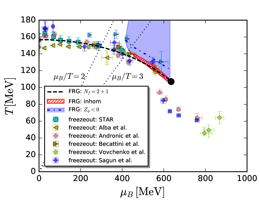
Figure 21: Phase diagram for $N_{f}=2+1$ flavour QCD in comparison to freeze-out data. The crossover temperature has been determined through the peak position of the thermal susceptibility of the renormalised light chiral condensate $\Delta_{l,R}$, see (133), (137): $\partial_{T}\Delta_{l,R}$ at fixed baryon chemical potential $\mu_{B}$. For more details see Section V. The phase boundary globally agrees well with recent lattice results, and in particular the curvature of the phase boundary for small chemical potential, $\kappa=0.0142(2)$, is consistent with recent lattice results. We find a critical end point at $(T_{\text{\tiny CEP}},{\mu_{B}}_{\text{\tiny CEP}})=(107,635)\,\text{MeV}$.
fRG: inhom: The blue area depicts the regime with a negative slope of the mesonic dispersion at vanishing spatial momentum, that is $Z_{\phi}(0)<0$, see Figure 12. There, the the meson dispersion has a minimum at a nonvanishing spatial momentum. This is a strong indication for an inhomogeneous regime. We also show the minimum of $Z_{\phi}(0)$ in $T$ at a fixed value of $\mu_{B}$ with the blue dashed line. The red hatched area shows where the inhomogeneous regime overlaps with a sizable homogeneous chiral condensate. The latter is defined as the size of the (reduced) chiral condensate where the thermal susceptibility $\partial\Delta_{l,R}/\partial T$ at fixed $\mu_{B}$ reaches 80$\%$ of its peak height (from above), and larger. In this region, a competition between homogeneous and inhomogeneous condensation is expected and the phase structure could be altered significantly. For a detailed discussion see Section V.2.
Freeze-out data: Adamczyk et al. (2017) (STAR), Alba et al. (2014) (Alba et al.), Andronic et al. (2018) ( Andronic et al.), Becattini et al. (2017) (Becattini et al.), and Vovchenko et al. (2016) (Vovchenko et al.). Note that freeze-out data from Becattini et al. with (blue) and without (dark green) afterburning corrections are shown in two different colors.

In turn, for chemical potentials above the regime in (130) either a CEP has already been observed or the standard chiral symmetry breaking pattern has broken down. For the upper bound on the CEP region we therefore assume that the system does not enter the critical region in the vicinity of the CEP we find here. A simple estimate of the phase boundary without a CEP at $(T_{\text{\tiny CEP}},{\mu_{B}}_{\text{\tiny CEP}})=(107,635)\,\text{MeV}$ is then given by an extrapolation of the boundaries of the width of the chiral transition in Figure 20 from the crossover region towards larger $\mu_{B}$. The intersection of these boundaries then yields the r.h.s. of (130). To be more specific, we fit the upper and lower bound of the width of the (2+1)-flavour chiral phase boundary in Figure 20 by the polynomial in (122) up to fourth order for chemical potentials $\mu_{B}\leq 630$ MeV. The two curves intersect at $(103,660)$ MeV.

We emphasise again, that these considerations are only the first step towards a combined functional analysis of the CEP. Moreover, (130) should be rather seen as the regime with either a CEP or interesting new phenomena such as a phase with an inhomogeneous condensate. As already mentioned in the beginning of this Section, in particular the present estimate is based on a linear error analysis in a nonlinear problem and hence has to be taken with a grain of salt. Despite the obvious deficiencies of the present analysis this combined functional approach at large chemical potential, while also utilising benchmark results from lattice simulations at smaller chemical potential will finally enable us to provide quantitative predictions for the large density regime including the potential CEP in the next few years.

VII Summary and outlook

In this work we have studied the QCD phase structure at finite temperature and baryon chemical potential as it emerges from the fundamental dynamics of QCD. To this end, we extended the dynamical hadronisation technique within the functional renormalisation group approach to QCD towards the inclusion of in-medium effects. Our results therefore constitute a new state-of-the-art regarding the understanding of the QCD phase diagram based on the dynamics of quarks and gluons.

We have investigated various quantities, including their temperature and chemical potential dependence. In particular, we have computed order parameters for chiral symmetry breaking, e.g. the renormalised chiral condensate, see Figure 10, as well as the Polyakov loop expectation value, see Figure 7. In addition, we studied the constituent quark mass, the pion and $\sigma$-meson masses, the wave function renormalisations/propagators, the running strong couplings and the interactions of quarks and the mesonic low energy degrees of freedom. This allowed us to gain insights into the interplay of different degrees of freedom at different momentum-, temperature- and density-scales.

Most importantly, we have obtained the phase diagram of $N_{f}=2$ and $N_{f}=2+1$ flavour QCD at finite temperature and baryon chemical potential, see Section V.4. Various aspects of our results, including comparisons to other recent works, are shown in Figures 1, 20 and 21. Our result for the curvature of the phase boundary for $2\!+\!1$ quark flavours at small chemical potential is $\kappa_{{}_{\tiny{N_{f}=2+1}}}=0.0142(2)$, which is fully compatible with the most recent lattice results Bellwied et al. (2015); Bazavov et al. (2019). In addition, we find a critical end point at $(T_{{}_{\tiny{\text{CEP}}}},{\mu_{B}}_{{}_{\tiny{\text{CEP}}}})=(107,635)$ MeV. We compare our results for $N_{f}=2+1$ and $N_{f}=2$ in Figure 20. Owing to strange quark fluctuations, the (2+1)-flavour phase boundary is systematically lower than the two-flavour boundary.

An intriguing aspect of our results is that we find strong indications for an inhomogeneous regime at large chemical potentials in the region $\mu_{B}\gtrsim 420$ MeV, shown in Figures 1 and 21. Since this regime intersects the phase boundary, it could have important implications for the QCD phase structure. For a detailed discussion see Section V.2.

A preliminary analysis of the systematic error in our computation is done in Section VI. In combination with a similar analysis of the DSE as well as with the benchmark results from the lattice at small chemical potential, we put forward a first suggestion for the region of the critical end point, see (130). This combination of results from functional approaches at large chemical potential and lattice results at small chemical potential will finally allow us to pin down the location of CEP or, given potential inhomogeneous phases and their implications, the onset of a new state of matter at large density.

This calls for a systematic improvement of the approximations used here. Firstly, only quark-antiquark scattering in the $\sigma$-$\pi$ channel has been taken into account for the dynamical hadronisation. Other channels, however, may play a sizable r$\hat{\textrm{o}}$le in particular at large $\mu_{B}$, such as diquark and vector-meson channels, see, e.g., Braun et al. (2017, 2018). Therefore, the present approximation for the four-quark couplings is currently extended to a Fierz-complete basis, see Mitter et al. (2015); Braun et al. (2017, 2018); Cyrol et al. (2018a). In addition, we need to allow for inhomogeneous quark-antiquark scattering channels in order to supplement our present results in this direction. Secondly, we have employed a minimal extension to include strange quark dynamics in our calculation. In the current work we have been concentrating on specific light quark observables which are insensitive to the details of the strange sector. However, this is insufficient for the highly interesting investigations of strangeness at finite chemical potential and temperature; for an fRG point of view see Fu et al. (2018a, b). For these aspects a full (2+1)-flavour study, including the corresponding four-quark interactions and resonances, is required. Finally, we relied on external input for the momentum-dependent gluon and ghost propagators in vacuum, the in-medium screening of gluons in Yang-Mills theory and the gauge part of the gluon effective potential. Only the average momentum dependences encoded in the cutoff dependence have been considered. Full momentum dependences have so far been considered in vacuum QCD and finite temperature Yang-Mills theory, Mitter et al. (2015); Braun et al. (2016a); Cyrol et al. (2016, 2018a, 2018b). Its extension to QCD at finite temperature and chemical potential is under way. This also includes a complete basis of tensor structures for in particular the quark-gluon vertex as well as the purely gluonic vertices. The selfconsistent determination of the gluon effective potential along the lines of Braun et al. (2010a) is also on our agenda.

Further interesting applications of the present work are manifold. In the following, we list selected active projects within the fQCD collaboration Braun et al. (2019c). A detailed study of QCD thermodynamics and the equation of state is the most obvious application. This will provide input for phenomenological studies of heavy-ion collisions that is firmly rooted in QCD even at small beam energies. Since the chiral limit is easily accessible within the present approach, the magnetic equation of state is also being computed. Furthermore, fluctuations and correlations of conserved charges are evaluated. The present approach allows for both, the spectral reconstruction and the direct computation of real-time correlation functions in QCD along the lines of Floerchinger (2012); Strauss et al. (2012); Haas et al. (2014); Kamikado et al. (2014); Silva et al. (2014); Christiansen et al. (2015); Pawlowski and Strodthoff (2015); Jung et al. (2017); Pawlowski et al. (2018); Cyrol et al. (2018c); Tripolt et al. (2018b); Dudal et al. (2019); Binosi and Tripolt (2019); Li et al. (2019b), that are important for QCD-assisted transport, Bluhm et al. (2019), and QCD-assisted hydrodynamics, Dubla et al. (2018). These applications play important r$\hat{\textrm{o}}$les in experimental searches for the CEP, and more generally for our understanding of the QCD phase structure. We hope to report on these matters in the near future.

Appendix A Chiral condensates

Here we explain of how to extract chiral condensates within the present approach. Results in the present approximations for the renormalised chiral condensate, (133), and the reduced chiral condensate, (134), are presented in Figure 22 and Figure 23 respectively.

Naturally, these observables are derived from the thermodynamic potential density or free energy density defined in (67), evaluated on the EoM (6) with $J=0$. This is a finite, renormalisation group invariant observable, as follows from its relation to the effective action $\Gamma[\Phi_{\textrm{EoM}}]$. The chiral condensates are proportional to $\int_{x}\langle\bar{q}_{i}q_{i}\rangle$ with $q_{i}=u,d,s$ and vanishes in the chirally symmetric regime. Up to the normalisation it is given by the derivative of $\Gamma$ w.r.t. the current quark mass $m^{0}_{q_{i}}$, to wit

$$\Delta_{q_{i}}= \,m_{q_{i}}^{0}\frac{\partial\Omega[\Phi_{\textrm{EoM}};T,\mu_{q}]}{\partial{m^{0}_{q_{i}}}}=m_{q_{i}}^{0}\frac{T}{\cal V}\int_{x}\langle\bar{q}_{i}(x)q_{i}(x)\rangle\,,$$ (131)

where no sum over $i$ is implied in (131). The normalisation in (131) includes the trivial volume factor $T/{\cal V}$ with the spatial volume $\cal V$. The multiplication factor $m_{q_{i}}^{0}$ leading to the logarithmic current quark masses derivative removes possible ambiguities relative to the condensates from other formulations such as DSEs and the lattice. In the present work the masses of the light quarks $u,d$ are the same, $m_{u}=m_{d}=m_{l}$, and we define the light quark condensate $\Delta_{l}=\Delta_{u}=\Delta_{d}$. Up to renormalisation terms the condensates $\Delta_{q_{i}}$ read

$$\Delta_{q_{i}}\simeq-m_{q_{i}}^{0}T\sum_{n\in\mathbb{Z}}\int\frac{d^{3}q}{(2\pi)^{3}}\operatorname{tr}\,G_{q_{i}\bar{q}_{i}}(q)\,.$$ (132)

The necessity of the renormalisation of (132) is typically circumvented by subtracting two condensates from each other. One convenient choice is to only consider the thermal and density part of the condensates, similar to the definition of the pressure $p=-(\Omega[\Phi_{\textrm{EoM}};\mu_{q},T]-\Omega[\Phi_{\textrm{EoM}};0,0])$. This leads us to the renormalised condensate $\Delta_{q_{i},R}$ with

$$\Delta_{q_{i},R}=\frac{1}{{\cal N}_{R}}\left[\Delta_{q_{i}}(T,\mu_{q})-\Delta_{q_{i}}(0,0)\right]\,.$$ (133)

Indeed, $\Delta_{q_{i},R}=-m^{0}_{q_{i}}\partial_{q_{i}}p$. In (133) the normalisation ${\cal N}_{R}$ renders $\Delta_{q_{i},R}$ dimensionless. ${\cal N}_{R}$ is a convenient normalisation that is typically chosen to be one of the characteristic, well-determined, scales in the theory. A common choice is ${\cal N}_{R}=m_{\pi}^{4}$ for the physical case. If also being interested in the chiral limit, ${\cal N}_{R}=f_{\pi}^{4}$ is better suited.

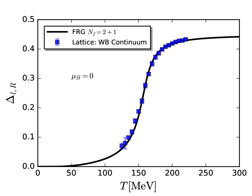
Figure 22: $N_{f}=2+1$ renormalised light chiral condensate $\Delta_{l,R}$, in Eqs. (133) and (137) as a function of the temperature with $\mu_{B}=0$, in comparison to the lattice result in Borsanyi et al. (2010). The normalisation constant in (133) and (137) is chosen to match the scale in the lattice calculation.

Another common choice is the reduced condensate $\Delta_{l,s}$, which is proportional to the weighted difference between light and strange quark condensate, $\Delta_{l}$ and $\Delta_{s}$. It is normalised by its value in the vacuum and reads

$$\Delta_{l,s}(T,\mu_{q})=\frac{\Delta_{l}(T,\mu_{q})-\left(\frac{m_{l}^{0}}{m_{s}^{0}}\right)^{2}\Delta_{s}(T,\mu_{q})}{\Delta_{l}(0,0)-\left(\frac{m_{l}^{0}}{m_{s}^{0}}\right)^{2}\Delta_{s}(0,0)}\,.$$ (134)

In the functional RG approach the necessity of renormalising (132) is resolved by the very definition (131) to use current quark mass derivatives of the the basic object in the approach, the finite effective action $\Gamma[\Phi_{\textrm{EoM}}]$: We first use that $\Delta_{l}$ can be represented as a $c_{\sigma}$-derivative,

$$\Delta_{l}=\frac{1}{2}m_{l}^{0}\frac{\partial\Omega[\Phi_{\textrm{EoM}};T,\mu_{q}]}{\partial{m_{l}^{0}}}=\frac{1}{2}c_{\sigma}\frac{\partial\Omega[\Phi_{\textrm{EoM}};T,\mu_{q}]}{\partial{c_{\sigma}}}\,,$$ (135)

where we have used that $c_{\sigma}\propto m_{l}^{0}$ carries the only dependence of $\Omega$ on the current quark mass $m_{l}^{0}$. This leads us to the finite chiral condensate

$$\Delta_{l}(T,\mu_{q})=-\frac{1}{2}c_{\sigma}\,\sigma_{\textrm{EoM}}(T,\mu_{q})\,,$$ (136)

which is simply the term in the effective action that explicitly breaks chiral symmetry. We emphasise that (136) is an exact relation. Using (136) in (133) we arrive at

$$\Delta_{l,R}(T,\mu_{q})=-\frac{c_{\sigma}}{{2\,\cal N}_{R}}\left[\sigma_{\textrm{EoM}}(T,\mu_{q})-\sigma_{\textrm{EoM}}(0,0)\right]\,.$$ (137)

This is readily computed within the present approach. In Figure 22 we show the results within the current approximation in comparison to the continuum extrapolated lattice result in Borsanyi et al. (2010), for results at finite baryon chemical potentials see Figure 10 in Section V.1. The normalisation constant in (133) and (137) is chosen to match the scale in the lattice calculation.

In an approach with (dynamical) hadronisation also for the strange quark sector also the reduced condensate can be represented in terms of the meson field expectation values. Similarly to (135) we get

$$\Delta_{s}=m_{s}^{0}\frac{\partial\Omega[\Phi_{\textrm{EoM}};T,\mu_{q}]}{\partial{m_{s}^{0}}}=c_{\sigma_{s}}\frac{\partial\Omega[\Phi_{\textrm{EoM}};T,\mu_{q}]}{\partial{c_{\sigma_{s}}}}\,,$$ (138)

leading to

$$\Delta_{s}(T,\mu_{q})=-\frac{1}{\sqrt{2}}c_{\sigma_{s}}\,\sigma_{s,\textrm{EoM}}(T,\mu_{q})\,.$$ (139)

With (136) and (139) we arrive at

$$\Delta_{l,s}(T,\mu_{q})=\frac{\left(\sigma-\sqrt{2}\frac{c_{\sigma}}{c_{\sigma_{s}}}\sigma_{s}\right)_{T,\mu_{q}}}{\left(\sigma-\sqrt{2}\frac{c_{\sigma}}{c_{\sigma_{s}}}\sigma_{s}\right)_{0,0}}\,,$$ (140)

where we have used that

$$\frac{m_{l}^{0}}{m^{0}_{s}}=\frac{c_{\sigma}}{c_{\sigma_{s}}}\,,$$ (141)

see also (47) and Section III.3 for its derivation. It is implicitly understood that $\sigma$ and $\sigma_{s}$ in (140) are evaluated on the respective EoMs.

In the current work we utilise the simple approximation (49) for the respective strange condensate. Using (49) in the reduced condensate (140) leads us to the simple expression

$$\Delta_{l,s}(T,\mu_{q})=\frac{\sigma(T,\mu_{q})}{\sigma(0,0)}\frac{1-\frac{m_{l}^{0}}{m_{l}(T,\mu_{q})}}{1-\frac{m_{l}^{0}}{m_{l}(0,0)}}\,,$$ (142)

Notably, the explicit dependence on the current strange quark mass $m^{0}_{s}$ has dropped out. Equation (142) also makes evident that it is even nonvanishing in the flavour-symmetric case with $m_{l}^{0}=m_{s}^{0}$ even though both the numerator and the denominator in (140) vanish.

Equation (140) still contains explicitly the parameters of explicit chiral symmetry breaking in the initial action, $c_{\sigma},c_{\sigma_{s}}$. Now we rewrite (140) in terms of the full effective action $\Gamma_{k=0}$. To that end we utilise the equations of motion. For constant solutions $\sigma_{\textrm{EoM}},\sigma_{s,\textrm{EoM}}$ they read

$$\sigma_{\textrm{EoM}}= \,\frac{c_{\sigma}}{V^{(1,0)}_{k}(\rho_{\textrm{EoM}},\rho_{s,\textrm{EoM}})},$$

$$\sigma_{s,\textrm{EoM}}= \,\frac{1}{\sqrt{2}}\frac{c_{\sigma_{s}}}{V^{(0,1)}_{k}(\rho_{\textrm{EoM}},\rho_{s,\textrm{EoM}})}\,,$$ (143)

where $V^{(1,0)}_{k}(\rho,\rho_{s})=\partial_{\rho}V_{k}(\rho,\rho_{s})$ and $V^{(0,1)}_{k}(\rho,\rho_{s})=\partial_{\rho_{s}}V_{k}(\rho,\rho_{s})$. Inserting (143) for $k=0$ in (140) yields

$$\Delta_{l,s}=\left.\frac{\left(\frac{1}{m_{\pi}^{2}}-\frac{1}{V^{(0,1)}(\rho,\rho_{s})}\right)_{T,\mu_{q}}}{\left(\frac{1}{m_{\pi}^{2}}-\frac{1}{V^{(0,1)}(\rho,\rho_{s})}\right)_{0,0}}\right|_{\textrm{EoM}}\,,$$ (144)

where the fields $\rho,\rho_{s}$ are evaluated on the respective EoMs (143) at finite $T,\mu_{q}$ and in the vacuum. Equation (144) depends on the unrenormalised pion mass $m_{\pi}^{2}=V^{(1,0)}(\rho_{\textrm{EoM}})$, and the effective potentials in (144) are evaluated at vanishing cutoff scale, $V(\rho,\rho_{s})=V_{k=0}(\rho,\rho_{s})$. Equation (144) only depends on the full effective potential at vanishing cutoff scale $k=0$: the apparent dependence on the parameters of the initial effective action has been removed. In the chiral limit both the numerator and the denominator of the reduced condensate vanish as they should. A convenient reparameterisation of (144) leads us to

$$\Delta_{l,s}=\left.\frac{\sigma(T,\mu_{q})}{\sigma(0,0)}\frac{1-\left[\frac{V^{(1,0)}(\rho,\rho_{s})}{V^{(0,1)}(\rho,\rho_{s})}\right]_{T,\mu_{q}}}{1-\left[\frac{V^{(1,0)}(\rho,\rho_{s})}{V^{(0,1)}(\rho,\rho_{s})}\right]_{0,0}}\right|_{\textrm{EoM}}\,.$$ (145)

Its computation only requires the knowledge of the full effective potential $V(\rho,\rho_{s})$ at vanishing cutoff scales at the $T,\mu_{q}$-dependent EoMs $\sigma_{\textrm{EoM}},\sigma_{s,\textrm{EoM}}$: the $T,\mu_{q}$-dependent pion and masses. The flow equation for the effective potential and the relevance analysis in Section V.3 and Appendices K, L allows us also to provide a simple expression for $V(\rho,\rho_{s})$. The effective potential is generated from the $\sigma,\sigma_{s}$ dependences of the Yukawa terms. These terms have the full $N_{f}$-symmetry which is unspoiled by the flow as neither $c_{\sigma}$ nor $c_{\sigma_{s}}$ are present. In the present approximation we only consider the diagonal terms in the full potential. This is consistent as long as the potential is mostly driven by the quark contribution: This approximation is well justified for larger temperatures and small baryon chemical potential, but may fail for larger chemical potential $\mu_{B}$ and small temperatures. This is one of the reasons why we do not consider the reduced condensate as an order parameter for chiral symmetry breaking here, its reliability at large $\mu_{B}$ requires a better approximation. In the present quark-dominated approximation the potential is simply a sum of the same potential $V_{k}$ for both $\rho$ and $\rho_{s}$ separately. This yields

$$V_{k}(\rho,\rho_{s})\approx V_{k}(\rho)+\frac{1}{2}V_{k}(2\rho_{s})\,,$$ (146)

which is a quantitative approximations for cutoff scales $k\gtrsim 200-300\,$MeV. With (146) we arrive at

$$\Delta_{l,s}=\left.\frac{\sigma(T,\mu_{q})}{\sigma(0,0)}\frac{1-\left[\frac{V^{\prime}(\rho)}{V^{\prime}(2\rho_{s})}\right]_{T,\mu_{q}}}{1-\left[\frac{V^{\prime}(\rho)}{V^{\prime}(2\rho_{s})}\right]_{0,0}}\right|_{\textrm{EoM}}\,,$$ (147)

Equation (147) can be evaluated within our current approximation, see Figure 23. Note that the reduced condensate, $\Delta_{l,s}$, in contradistinction to the renormalised condensate, $\Delta_{l,R}$, is sensitive to the correct relative treatment of strange and light quark sector. In the current work we have used a simple approximation for the strange quark sector as none of our observables is sensitive to the subleading differences between light quark and strange quark sector. Put differently, we may use the reduced condensate for fixing the strange current quark mass $m_{s}^{0}$ or $c_{\sigma_{s}}$, alternatively to the ratio of the decay constants $f_{K}/f_{\pi}$. Given the large value of the constituent strange quark mass in the Landau gauge, $m_{s}^{0}\gtrsim 500$  MeV, see e.g. Fischer (2019), we expect $m_{s}^{0}\gtrsim 150$  MeV for this adjustment, for a detailed discussion see Section III.3 around (47). There we also referred to the $N_{f}=2+1$ flavour ratio from lattice simulations, $f_{K}/f_{\pi}\approx 27$, which is obtained here for

$$\Delta\bar{m}_{sl}=150\,\textrm{MeV}\,,\quad c_{\sigma_{s}}=97.5\,{\textrm{GeV}}^{3}\,.$$ (148)

Note also that $c_{\sigma_{s}}$ and hence the ratio varies rapidly with $\Delta\bar{m}_{sl}$ from current quark mass ratios $m_{s}^{0}/m_{l}^{0}=c_{\sigma_{s}}/c_{\sigma}=14,27,30,34$ for $\Delta\bar{m}_{sl}=120,150,155,160$ MeV. While this has a minimal impact on the reduced condensate $\Delta_{l,s}$ at small temperatures this variation changes the temperature-dependence of $\Delta_{l,s}$ at large temperature. This is clearly seen in Figure 23. Note that while this strange quark mass variation has no impact on the light quark and gluon correlation functions and observables, it of course is relevant for observables and correlations with strange quark content. In particular we see quantitative agreement of the reduced condensate for all temperatures studied here for current quark ratios close to the physical one.

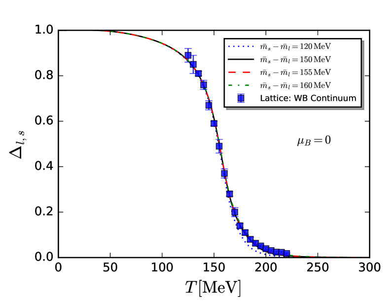
Figure 23: The reduced condensate in the approximation (147) for the constituent quark mass difference $\Delta\bar{m}_{sl}=\bar{m}_{s}-\bar{m}_{l}=120,150,155,160$ MeV for current quark mass ratios of $m_{s}^{0}/m_{l}^{0}=c_{\sigma_{s}}/c_{\sigma}\approx 14,27,30,34$ in comparison to the lattice results in Borsanyi et al. (2010). We observe quantitative agreement for all temperatures for ratios close to the physical one from $N_{f}=2+1$ flavour lattice simulations, $m_{s}^{0}/m_{l}^{0}\approx 27$ from Aoki et al. (2014).

We close this Appendix with a discussion of possible improvements of the computation of the condensates (or other observables) utilising the flow equation of the condensates instead of the their representation in terms of the effective action/potential at $k=0$. Such an improvement is based on the fact that in a given approximation each flow-step generates terms (information) that is dropped when projecting on the approximation of the effective action at hand. Accordingly, a flow representation of a specific observables may keep this information.

Of course, without approximation both ways have to give the same results, which can be cast in form of an integrability condition,

$$\left[\partial_{c_{\sigma}}\,,\,\partial_{t}\right]\,\Gamma_{k}[\Phi_{\textrm{EoM}}]\equiv 0\,,$$ (149)

for more details see Pawlowski (2007); Pawlowski et al. (2017); Braun et al. (2019a). While being trivial for the full theory, (149) is nontrivial within a given approximation. For the flow of the chiral condensate $\Delta_{q_{i}}$ we use the flow equation for the effective action,

$$\partial_{t}\Delta_{q_{i}}= \,m^{0}_{q_{i}}\frac{\partial}{\partial m^{0}_{q_{i}}}\partial_{t}\Gamma[\Phi_{\textrm{EoM}}]$$

$$= \,\frac{1}{2}m^{0}_{q_{i}}\frac{\partial}{\partial m^{0}_{q_{i}}}\Bigl{(}\operatorname{Tr}\,G_{k}[\Phi_{\textrm{EoM}}]\,\partial_{t}R_{k}\Bigr{)}\,.$$ (150)

Note that all the dynamical hadronisation terms in the flow vanish on the equation of motion within our choice as $\langle\partial_{t}\hat{\phi}_{k}\rangle_{\textrm{EoM}}=0$. Seemingly, (150) carries explicit and implicit dependences on the current quark mass. The implicit ones are that of the $\Phi_{\textrm{EoM}}$ and that of the couplings. The latter dependences can be computed with the same recursive relations as has been put forward in Fu and Pawlowski (2015) for the $\mu_{q}$-dependence. However, (150) can be simplified with (135), and we write for the light quark condensate

$$\partial_{t}\Delta_{l}= \,\frac{1}{2}\,c_{\sigma}\partial_{c_{\sigma}}\partial_{t}\Gamma[\Phi_{\textrm{EoM}}]$$

$$= \,\frac{1}{4}\,c_{\sigma}\partial_{c_{\sigma}}\Bigl{(}\operatorname{Tr}\,G_{k}[\Phi_{\textrm{EoM}}]\,\partial_{t}R_{k}\Bigr{)}$$

$$= \,\frac{1}{4}\,c_{\sigma}\int_{x}\frac{\partial\Phi_{\textrm{EoM}}}{\partial{c_{\sigma}}}\frac{\delta}{\delta\Phi}\left.\Bigl{(}\operatorname{Tr}\,G_{k}[\Phi]\,\partial_{t}R_{k}\Bigr{)}\right|_{\Phi_{\textrm{EoM}}}\,,$$ (151)

where we have used that the diagrams depends on $c_{\sigma}$ only via the equations of motion $\Phi_{\textrm{EoM}}$. As in (150) all the dynamical hadronisation terms in the flow vanish on the equation of motion within our choice as $\langle\partial_{t}\hat{\phi}_{k}\rangle_{\textrm{EoM}}=0$. For the strange quark condensate we get

$$\partial_{t}\Delta_{s}=\,\frac{1}{2}\,c_{\sigma_{s}}\int_{x}\frac{\partial\Phi_{\textrm{EoM}}}{\partial{c_{\sigma_{s}}}}\frac{\delta}{\delta\Phi}\left.\Bigl{(}\operatorname{Tr}\,G_{k}[\Phi]\,\partial_{t}R_{k}\Bigr{)}\right|_{\Phi_{\textrm{EoM}}}\,,$$ (152)

The only nonvanishing solutions of the EoM are $\sigma_{\textrm{EoM}}$, $\sigma_{s,\textrm{EoM}}$ and $L_{\textrm{EoM}},\bar{L}_{\textrm{EoM}}$. In a further approximation we only consider the direct contributions and neglect the subleading dependencies of $\sigma_{s},L,\bar{L}$ on $c_{\sigma}$ via the change of $\sigma_{\textrm{EoM}}$, as well as that of $\sigma,L,\bar{L}$ on $c_{\sigma_{s}}$ via the change of $\sigma_{s,\textrm{EoM}}$,

$$\frac{\partial(\sigma_{s},L,\bar{L})_{\textrm{EoM}}}{\partial c_{\sigma}}\approx 0\approx\frac{\partial(\sigma,L,\bar{L})_{\textrm{EoM}}}{\partial c_{\sigma_{s}}}\,.$$ (153)

In the current approximation this leads us to

$$\partial_{t}\Delta_{l}=\frac{c_{\sigma}}{2}\frac{\partial\sigma_{\textrm{EoM}}}{\partial{c_{\sigma}}}\,\partial_{\sigma}\left[\frac{1}{2}\,\operatorname{Tr}\,G_{\phi\phi}\,\partial_{t}R_{\phi}-\operatorname{Tr}\,G_{q\bar{q}}\,\partial_{t}R_{q}\right]\,,$$ (154)

and

$$\partial_{t}\Delta_{s}=\,c_{\sigma_{s}}\frac{\partial\sigma_{s,\textrm{EoM}}}{\partial c_{\sigma_{s}}}\,\partial_{\sigma_{s}}\left[\frac{1}{2}\,\operatorname{Tr}\,G_{\phi\phi}\,\partial_{t}R_{\phi}-\operatorname{Tr}\,G_{q\bar{q}}\,\partial_{t}R_{q}\right]\,,$$ (155)

For the explicit result we first concentrate on the light condensate. Within the approximation (153) we get

$$c_{\sigma}\frac{\partial\Gamma^{(1)}_{\sigma}[\Phi_{\textrm{EoM}}]}{\partial c_{\sigma}}=\Gamma^{(2)}_{\sigma\sigma}[\Phi_{\textrm{EoM}}]\,c_{\sigma}\frac{\partial\sigma_{\textrm{EoM}}}{\partial{c_{\sigma}}}-c_{\sigma}=0\,,$$ (156)

Equation (156) leads us to

$$c_{\sigma}\frac{\partial\sigma_{\textrm{EoM}}}{\partial{c_{\sigma}}}=\frac{c_{\sigma}}{m_{\sigma}^{2}}\,,\quad\textrm{with}\quad m_{\sigma}^{2}=\left.\partial_{\sigma}^{2}V_{k}\right|_{\sigma_{\textrm{EoM}}}\,.$$ (157)

Collecting all the ingredients this leads us to

$$\partial_{t}\Delta_{l}= \,\frac{1}{2}\frac{c_{\sigma}}{m^{2}_{\sigma}}\Biggl{[}\frac{h_{k}}{2}\operatorname{Tr}G_{q\bar{q}}^{2}\,\partial_{t}R_{q}$$

$$\,-\frac{1}{2}\operatorname{Tr}\,\left(G_{\sigma\sigma}^{2}V^{(3)}_{\sigma\sigma\sigma}+G_{\pi\pi}^{2}V^{(3)}_{\sigma\pi\pi}\right)\,\partial_{t}R_{\phi}\Biggr{]}\,.$$ (158)

Note that the expression in the square bracket is nothing but $\partial_{\sigma}\dot{V}_{k}$ and $m_{\sigma}^{2}$ is the second $\sigma$-derivative of $V_{k}$, see (157). Now we use that the flow of $\sigma_{\textrm{EoM},k}$ follows straightforwardly from the cutoff dependence EoM $\partial_{\sigma}V_{k}=c_{\sigma}$. The $t$-derivative of the EoM reads

$$\partial_{t}\sigma_{\textrm{EoM},k}V^{(2)}_{k}+\partial_{t}V^{(1)}_{k}=0\,,$$ (159a)

which can be solved for the flow of $$\sigma_{\textrm{EoM},k}$$,

$$\to\partial_{t}\sigma_{\textrm{EoM},k}=-\left.\frac{\dot{V}_{k}^{(1)}}{{V_{k}^{(2)}}}\right|_{\sigma=\sigma_{\textrm{EoM},k}}\,.$$ (159b)

Accordingly, (158) is nothing but the flow of $\sigma_{\textrm{EoM},k}$ up to a prefactor $-c_{\sigma}$. This follows already from (136), to wit

$$\frac{1}{c_{\sigma}}\partial_{t}\Delta_{l}=-\frac{1}{2}\partial_{t}\sigma_{\textrm{EoM},k}\,,$$ (160)

which proves that (149) holds nontrivially in the present approximation. Note also that at large cutoff scales the term in the second line of (158) from the mesonic loop drops quickly proportional to $\sigma_{\textrm{EoM}}$. The prefactor of the first term approaches the current quark mass $\frac{c_{\sigma}\,h_{k}}{m^{2}_{\sigma}}\to 2m_{l}^{0}$. Hence, in this limit (158) reduces to the explicit $m_{l}^{0}$-derivatives in (150). In turn, for smaller cutoff scales (158) carries also the implicit ones in (150).

Appendix B Dynamical hadronisation

Here we carefully derive the hadronisation relations for the given hadronisation (15), which is recalled here,

$$\langle\partial_{t}\hat{\phi}_{k}\rangle= \dot{A}_{k}\,\bar{q}\tau q+\dot{B}_{k}\,\phi+\frac{1}{\sqrt{2N_{f}}}\dot{C}_{k}\hat{e}_{\sigma}\,,$$ (161)

with $\hat{e}_{\sigma}$ is a conveniently normalised vector in the $\sigma$-direction, $\hat{e}_{\sigma}^{2}=1/\sqrt{2N_{f}}$. Now we use the shift in the $\sigma$-direction, $\dot{C}_{k}(\Phi)\,\hat{e}_{\sigma}$, for absorbing the current quark mass of up- and down-quarks into the mesonic field. Here we allow a field dependence of the coefficient $\dot{C}_{k}$. Then, the scalar quark two-point function

$$(\bar{q}\tau^{0}q)=(\bar{u}u+\bar{d}d)/2\,,$$ (162)

is proportional to $\sigma$ and its symmetry part vanishes for all momenta $p$ and cutoff scales $k$,

$$\Gamma^{(2)}_{(\bar{q}\tau^{0}q)}[\sigma](p)+\Gamma^{(2)}_{(\bar{q}\tau^{0}q)}[-\sigma](p)\equiv 0\,.$$ (163)

This entails, that the flow of the symmetric part vanishes,

$$\partial_{t}\Gamma^{(2)}_{(\bar{q}\tau^{0}q)}[\sigma](p)+\partial_{t}\Gamma^{(2)}_{(\bar{q}\tau^{0}q)}[-\sigma](p)\equiv 0\,.$$ (164)

Moreover, it also leads to vanishing flow diagrams,

$$\textrm{Flow}^{(2)}_{(\bar{q}\tau^{0}q)}[\sigma](p)+\textrm{Flow}^{(2)}_{(\bar{q}\tau^{0}q)}[-\sigma](p)\equiv 0\,.$$ (165)

For the determination of $\dot{C}_{k}$ we evaluate the flow equation for the scalar part of the quark two point function, derived from (26) with the choice (161). It reads

$$\partial_{t}\Gamma_{(\bar{q}\tau^{0}q)}^{(2)}+\dot{A}_{k}\,\left(\frac{\delta\Gamma}{\delta\sigma}+c_{\sigma}\right)+\dot{C}_{k}\,\Gamma^{(3)}_{(\bar{q}\tau^{0}q)\sigma}=\textrm{Flow}^{(2)}_{(\bar{q}\tau^{0}q)}\,,$$ (166)

where the field-dependence of all correlation functions has been suppressed, and the subscript ${}_{(\bar{q}q)}$ indicates the projection on the scalar part of the quark two-point function $\bar{q}q=2\bar{q}\tau^{0}q$. Upon symmetrising (166) the flow of the quark two-point function, $\partial_{t}\Gamma_{(\bar{q}\tau^{0}q)}^{(2)}$ and the diagrams, $\textrm{Flow}^{(2)}_{(\bar{q}\tau^{0}q)}$, drop out due to (164), (165). This leaves us with

$$\dot{C}_{k}=-{\dot{A}_{k}}\,\frac{1}{\Gamma^{(3)}_{(\bar{q}\tau^{0}q)\sigma}[\sigma]}\,\frac{\Gamma^{(1)}_{\sigma}[\sigma]+\Gamma^{(1)}_{\sigma}[-\sigma]+2c_{\sigma}}{2}\,,$$ (167)

where we have used that (163) leads us to $\Gamma^{(3)}_{(\bar{q}\tau^{0}q)\sigma}[-\sigma]=\Gamma^{(3)}_{(\bar{q}\tau^{0}q)\sigma}[\sigma]$. In the chiral limit the numerator in (167) vanishes and $\dot{C}_{k}\equiv 0$ as expected. For finite current quark masses (167) the symmetric sum $\Gamma^{(1)}_{\sigma}[\sigma]+\Gamma^{(1)}_{\sigma}[-\sigma]=-2c_{\sigma}$. Hence, we finally conclude

$$\dot{C}_{k}\equiv 0\,.$$ (168)

This is the expected property following from the symmetry constraints on the $\sigma$-dependence we have imposed in (163), see also the discussion in Section II.1. With (168) we are led to

$$\partial_{t}\Gamma_{(\bar{q}\tau^{0}q)}^{(2)}+\dot{A}_{k}\,\left(\frac{\delta\Gamma}{\delta\sigma}+c_{\sigma}\right)=\textrm{Flow}^{(2)}_{(\bar{q}\tau^{0}q)}\,,$$ (169)

As (169) depends on $\Gamma^{(1)}_{\sigma}$, we also study the respective flow in order to discuss the selfconsistence of the current expansion schemes as well as the optimisation of the approximation (39) used in the present work. The flow of $\Gamma^{(1)}_{\sigma}$ at $(q,\bar{q})=0$ reads

$$\partial_{t}\Gamma_{\sigma}^{(1)}=\textrm{Flow}^{(1)}_{\sigma}\,,$$ (170)

and is that in the chiral limit: it does not depend on $c_{\sigma}$, see Section 52. Accordingly the dynamical hadronisation put forward here carries the full chiral symmetry at each cutoff scale due to the shift in $J_{\sigma}$. Explicit chiral symmetry breaking is entirely carried by the linear term in $\sigma$. Inserting (39) in (169), we arrive at

$$\partial_{t}h_{k}(\rho)+m_{\pi}^{2}(\rho)\,\dot{A}=\frac{1}{\sigma}\textrm{Flow}^{(2)}_{(\bar{q}\tau^{0}q)}\,,$$ (171)

where $m_{\pi}^{2}(\rho)=\partial_{\rho}V(\rho)$. In terms of dimensionless variables and after rescaling with the wave function renormalisations we are led to (115).

In summary we are left with the two key equations (170) and (171). In particular the latter one, (171), relates the $\rho$-dependence of the pion mass function $m_{\pi}^{2}(\rho)$ to that of the Yukawa coupling. This entails that the field-dependence of the Yukawa coupling is in one-to-one correspondence to that of the effective potential, see also Pawlowski and Rennecke (2014). Since we do not take into account the $\rho$-dependence of $h_{k}(\rho)$, the respective systematic error is minimised for an expansion point in the Taylor expansion in $\rho$, that minimises the higher Taylor coefficients of $m_{\pi}^{2}(\rho)$:

$$\min_{\rho}|\partial_{\rho}^{n}m_{\pi}^{2}(\rho)|=\min_{\rho}|\partial_{\rho}^{n+1}V(\rho)|\,.$$ (172)

The Taylor coefficients in (172) are minimised at the flowing minimum, the $k$-dependent EoM for $\kappa_{k}=\sigma^{2}_{\textrm{EoM},k}/2$. Note however that this expansion point does not lead to best convergence for the flow of the effective potential, (170). The latter flow shows best convergence for a fixed expansion point close to the final minimum $\sigma_{\textrm{EoM}}=\sigma_{\textrm{Eom},k=0}$. Accordingly, for small cutoff scales a fixed expansion point fares better than the running one in terms of convergence. It is suggestive to switch of the running of the renormalised expansion point at

$$\left.\partial_{t}\bar{\kappa}_{k}\right|_{k_{\textrm{peak}}}=0\,,\quad\textrm{with}\quad \bar{\kappa}_{k}=\bar{\rho}_{\textrm{EoM},k}\,,$$ (173)

see (117) in Section IV.4. However, if the frozen expansion point is too far away from the physical configuration $\rho_{\textrm{EoM}}=\bar{\rho}_{\textrm{EoM},k=0}\leq\bar{\rho}_{\textrm{EoM},k_{\textrm{peak}}}$, the latter may not be in the radius of convergence of the Taylor expansion. This is checked by stopping the flow of the minimum later and checking the stability of the results under this procedure. This subtlety can be avoided completely by a field-dependent Yukawa-coupling (and further field-dependent couplings such as the wave function renormalisations), see e.g. Pawlowski and Rennecke (2014). This will be studied in future work.

Appendix C Strange quark and the minimal extension to $N_{f}=2+1$

In this work we adopt an minimal approach to extend the calculation of $N_{f}=2$ to that of $N_{f}=2+1$. First of all, the contribution of the strange quark loop to the gluon anomalous dimension is included, i.e., another term denoted by $\eta_{A,k}^{s}$ is added in (100), which reads

$$\eta_{A,k}=\eta_{A,\textrm{vac}}^{\text{QCD}}+\Delta\eta_{A}^{\text{YM}}+\Delta\eta_{A}^{l}+\eta_{A}^{s}\,.$$ (174)

The in-medium gluon vacuum polarisation generated by the light quarks, $\Delta\eta_{A}^{l}$, is given by the in-medium part of (208) and (209) with $\bar{m}_{q}=\bar{m}_{l}$, $N_{f}=2$ and the light-quark–gluon coupling, $g_{\bar{l}Al}$, defined in (106) and (M). For the strange quark contribution, $\eta_{A}^{s}$, we use (208) directly with $\bar{m}_{q}=\bar{m}_{s}$, defined in (45), $N_{f}=1$ and the the strange-quark–gluon coupling, $g_{\bar{s}As}$, defined below. Note that $\eta_{A}^{s}$ not only contains the thermal contribution, as does $\Delta\eta_{A}^{q}$, but also includes the vacuum contribution, since our input for the unquenched QCD calculation in vacuum, i.e. the first term on the r.h.s. of (174), in only for two flavours Cyrol et al. (2018a).

Furthermore, the quark-gluon coupling for the strange quark is distinguished from that for the $u$- and $d$-quarks, and its flow equation is given by

$$\partial_{t}g_{\bar{s}As}= \left(\frac{1}{2}\eta_{A}+\eta_{q}\right)g_{\bar{s}As}+\overline{\textrm{Flow}}^{(3),A}_{(\bar{s}As)}\,.$$ (175)

where the last term is defined in (223). In comparison to (106), we note that in (175) we have neglected the contribution of mesonic fluctuations to the running of $g_{\bar{s}As}$. This will be improved in our future work. All explicit expressions for the quantities discussed here are given in Appendix H and M.

Appendix D Direct sum versus full back coupling

Here, we motivate the approximation we use for the gauge field propagator. The goal is to find a simple, yet quantitatively reliable scheme. This discussion is largely based on Braun et al. (2016a); Rennecke (2015b) and reiterated here for completeness. The most prominent feature in the gauge sector is confinement. In linear covariant gauges it manifests itself in the emergence of a gluon mass gap, cf. (32), together with an enhanced ghost propagator in the IR Gribov (1978); Kugo and Ojima (1979); Zwanziger (2004). This implies that in order to capture the mass gap, the full momentum dependence of the gauge field propagators has to be resolved. This is a formidable task which requires sophisticated truncation schemes and considerable numerical effort, e.g. Fischer et al. (2009); Aguilar et al. (2008); Boucaud et al. (2008); Fister and Pawlowski (2011); Mitter et al. (2015); Cyrol et al. (2016, 2018b). Here, we motivate an approximation scheme which uses the full gauge field propagators from fist-principles computations of the pure gauge theory as input, while matter effects, i.e. quark and hadron fluctuations, and their backreaction on the gauge sector, are computed selfconsistently.

Within the truncation scheme described in Section III, the propagators enter the flow equations through the corresponding anomalous dimensions and mass parameters. The gluon anomalous dimension, for instance, is in general a function of the strong couplings and the mass gap,

$$\eta_{A,k}^{\text{QCD}}=\eta_{A,k}^{\text{QCD}}(\alpha_{\bar{q}Aq},\alpha_{\bar{c}Ac},\alpha_{A^{3}},\alpha_{A^{4}},\bar{m}_{A}^{2},\bar{m}_{q}^{2})\,,$$ (176)

where we omitted the $k$-dependence on the couplings and masses for the sake of brevity. Within both, the fRG and DSE approaches this can always be split into a part where only diagrams of the pure gauge theory contribute, $\eta^{\textrm{glue}}(\alpha_{\bar{c}Ac},\alpha_{A^{3}},\alpha_{A^{4}},\bar{m}_{A}^{2})$, and the matter contribution, $\eta^{\textrm{quark}}_{A}(\alpha_{\bar{q}Aq},\bar{m}_{q}^{2})$. We note that the couplings themselves are the ones of QCD, i.e. the couplings in the gauge sector also depend on the ones in the matter sector and vice versa. Hence, the splitting of the gluon anomalous dimension into gauge and matter part is purely formal. A first simplification can be made by using that the different gauge couplings only differ from each other in the low-energy regime where the mass gap is generated, i.e. where gluons decouple in QCD. Hence, we parametrise the anomalous dimension as

$$\eta_{A,k}^{\text{QCD}}=\eta^{\textrm{glue}}_{A}(\alpha_{s},\bar{m}_{A}^{2})+\eta^{\textrm{quark}}_{A}(\alpha_{\bar{q}Aq},\bar{m}_{q}^{2})\,,$$ (177)

where $\alpha_{s}$ stands for $\alpha_{c\bar{c}A}$, $\alpha_{A^{3}}$ or $\alpha_{A^{4}}$. Note that the gluon mass gap is part of the gauge contribution. As discussed in Section III, the glue diagrams of the anomalous dimension in Yang-Mills theory and in QCD agree, and it can be parameterised in terms of the couplings $\alpha_{s}$ and the mass gap $m_{A}^{2}$. Accordingly, the differences between the glue parts in QCD and Yang-Mills theory come from the differences in $\alpha_{s}$ and $m_{A}^{2}$. We have

$$\left.\eta_{A}^{\textrm{glue}}\right|_{\textrm{YM}}= \,\eta_{A,k}^{\textrm{YM}}=\eta_{A}^{\textrm{glue}}\left(\alpha^{\textrm{YM}},(\bar{m}^{\textrm{YM}}_{A})^{2}\right)\,,$$

$$\left.\eta_{A}^{\textrm{glue}}\right|_{\textrm{QCD}}= \,\eta_{A}^{\textrm{glue}}\left(\alpha_{s},\bar{m}_{A}^{2}\right)\,,$$ (178)

where $\alpha_{s}$ and $m_{A}^{2}$ are the QCD couplings and mass gap respectively. This suggest a possible approximation scheme for the gluon propagator: One takes the Yang-Mills anomalous dimension $\eta_{A}^{\text{YM}}$ in (178) as an external input from a first-principles computation, computes $\alpha_{s}$, $\bar{m}_{A}^{2}$ and $\eta_{A}^{\textrm{quark}}(\alpha_{\bar{q}Aq},\bar{m}_{q}^{2})$ as functions of the RG scale $k$ and puts everything together according to (177).

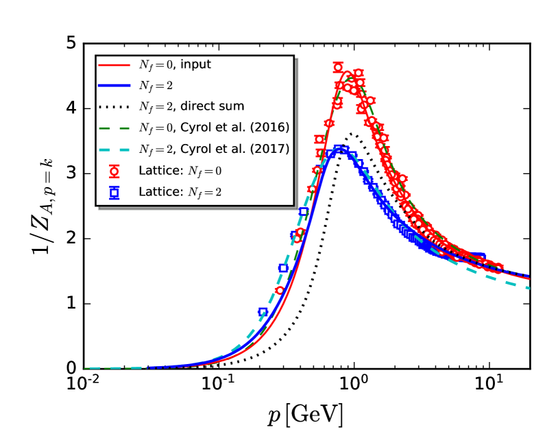
Figure 24: Comparison between the $N_{f}=2$ propagators obtained from lattice gauge theory and fRG results at vanishing temperature and density. The solid red thin line shows the gluon propagator of the pure gauge theory we use as input. The open red circles are the corresponding lattice results Sternbeck et al. (2006). The blue open squares are the lattice results for two-flavour QCD Sternbeck et al. (2012). The solid blue thick line shows the fRG result using (177) and the dotted black line shows the result based on (179). Both results are taken from Braun et al. (2016a); Rennecke (2015b). Furthermore, results from the fRG calculations with the state-of-the-art truncations at vacuum for the pure Yang-Mills theory Cyrol et al. (2016) and $N_{f}=2$ unquenched QCD Cyrol et al. (2018a) are shown for comparison, which are denoted by the green and cyan dashed lines, respectively.

The advantage of this procedure is that the information about the full momentum dependence, and in particular the emergent mass gap, is encoded in the quantitatively reliable external input. The corrections from matter fluctuations as well as their feedback on the gauge contribution are computed ‘locally’, i.e. the full RG scale dependence of the correlation functions is resolved, but only one momentum configuration (typically vanishing momenta) is taken into account. A simple reduction of this procedure is to ignore the feedback from the matter sector onto the gauge sector and simply define

$$\eta_{A,k}^{\text{QCD}}=\eta_{A,k}^{\text{YM}}+\eta_{A,k}^{\textrm{quark}}(\alpha_{\bar{q}Aq},\bar{m}_{q}^{2})\,.$$ (179)

This amounts to only adding the gluon vacuum polarisation to the input from YM.

To check the quality of both approximations we compare the resulting gluon propagators to results from lattice gauge theory Sternbeck et al. (2006, 2012) at vanishing temperature and chemical potential in Figure 24. In this figure we also show the benchmark fRG calculations with the state-of-the-art truncation of pure Yang-Mills theory in vacuum, Cyrol et al. (2016), (thin green dashed line), and $N_{f}=2$ flavour QCD Cyrol et al. (2018a) (thick cyan dashed line). The fRG results in the current approximation have been taken from Braun et al. (2016a); Rennecke (2015b): The red line shows the input propagator from the pure gauge theory. The open circles are the corresponding lattice data in Sternbeck et al. (2006). The open blue squares show the lattice results for two-flavour QCD Sternbeck et al. (2012). The solid blue line shows our results within the approximation based on (177). We used $\alpha_{s}=\alpha_{\bar{c}Ac}$.

Indeed, this approximation leads to a perfect agreement with the corresponding lattice results. To facilitate a comparison between $p$- and $k$-dependent quantities, we have identified $k=p$. Note that the momentum scale is arbitrary here. If the feedback to the gauge sector is ignored, i.e. the approximation in (179) is used, we find the dotted black line in Figure 24. While it still is a good approximation to the full propagator, it is clearly outperformed by (177).

This results motivates the use of a local approximation, i.e. resolving only the RG scale dependence of the correlation functions, for the effects of matter fluctuations, as long as the relevant nonlocal information, i.e. the genuine momentum dependence, is taken into account through the input. This is crucial for the present work, since we compute the thermal and density corrections to the gluon vacuum polarisation in a local approximation directly, while we use the gluon anomalous dimension of QCD at $T=0$ as well as the thermal effects of YM as input, cf. (100).

Appendix E Initial conditions & infrared enhancement

E.1 Initial conditions

The UV cutoff scale where the flow for the effective action $\Gamma_{k}[\Phi]$, or rather that of the correlation functions $\Gamma^{(n)}_{k}[\Phi]$, is initiated, is chosen as

$$\Lambda=20\,\text{GeV}\,.$$ (180)

At this scale, only the fundamental couplings of QCD, i.e. the strong coupling and the quark masses, are relevant. We initiate the flow with a nonvanishing strong coupling $\alpha_{s}$,

$$\alpha_{\bar{q}Aq,\Lambda}=\alpha_{A^{3},\Lambda}=\alpha_{A^{4},\Lambda}=\alpha_{\bar{c}Ac,\Lambda}=\alpha_{s,\Lambda}\,,$$ (181)

such that all avatars of the strong coupling agree at the initial scale. The initial strong coupling $\alpha_{s}(\Lambda)$ is constrained by the requirement of the RG consistency in (112), and we find that (112) is satisfied for

$$\left.\alpha_{s,\Lambda}\right|_{N_{f}=2+1}=0.235\,,\qquad\left.\alpha_{s,\Lambda}\right|_{N_{f}=2}=0.21\,.$$ (182)

The only other input at our perturbative initial scale are the current quark masses. We identify the up and down quark masses, $m_{u}=m_{d}=m_{q}$, and fix their value by the pion mass in the vacuum to be $m_{\pi}=138$  MeV. Following our discussion in Section IV.1.1, we emphasise that the curvature mass $\bar{m}_{\pi}$ of the pion has been shown to be in very good agreement with the pion pole mass $m_{\pi,\textrm{pol}}$ defined by $\Gamma^{(2)}_{\pi\pi}(p^{2}=-m^{2}_{\pi,\textrm{pol}})=0$, see Helmboldt et al. (2015); Pawlowski et al. (2018). This can be traced back to the mild momentum dependence of the pion correlation function, Helmboldt et al. (2015); Mitter et al. (2015); Cyrol et al. (2018a) as well as its relatively small width. For the $\sigma$ resonance this is less obvious and in particular the width is not expected to be small. Accordingly the curvature mass $m_{\sigma}$ may not be close to the position of the smallest scalar resonance. In the present work it is computed to be $m_{\sigma}=485$  MeV. As discussed in Section III, the light quark mass is absorbed in a shift in the $\sigma$-field and simply leads to a linear term in the potential, $c_{\sigma}\,\sigma$, see Section III.3. We arrive at

$$c_{\sigma}=3.6\,\textrm{GeV}^{3}\,,\quad\;\textrm{with }\quad\;m_{\pi,k=0}=137\,\textrm{MeV}\,.$$ (183)

Note that $\bar{c}_{\sigma,k}=c_{\sigma}/Z_{\phi,k}^{1/2}$ with $c_{\sigma}$ being independent of $k$. This leads to

$$\partial_{t}\bar{c}_{k}=\frac{\eta_{\phi,k}}{2}\,\bar{c}_{k}\,.$$ (184)

The strange current quark mass is fixed as $m_{s,\Lambda}=120$  MeV by the ratio $f_{K}/f_{\pi}$, see the discussion in Section III.3 and Table 1. This amounts to

$$c_{\sigma_{s}}=48.8\,\textrm{GeV}^{3}\,,\quad\;\textrm{with }\quad\;\Delta\bar{m}_{sl}=120\,\textrm{MeV}\,.$$ (185)

We have checked that a variation of the difference of the constituent quark masses $100\,\textrm{MeV}\lesssim\Delta\bar{m}_{sl}\lesssim 200$ MeV does not influence our results for light quark and gluon correlation functions and observables.

In the perturbative regime all other couplings are irrelevant, so they are either vanishing or have irrelevant RG flows. This entails in particular that the full four-quark coupling $\bar{\lambda}_{q,\textrm{eff}}$ (that on the EoM for $\phi$) should be infinitesimally small,

$$\bar{\lambda}_{q,\textrm{eff}}=\frac{\bar{h}_{\Lambda}^{2}}{2\bar{m}_{\phi,\Lambda}^{2}}\approx 0\,.$$ (186)

where we have used the trivial initial effective potential

$$\bar{V}_{\Lambda}(\bar{\rho}) =\bar{m}^{2}_{\phi,\Lambda}\bar{\rho}\,.$$ (187)

Equation (186) fixes the ratio of the meson mass parameter and the Yukawa coupling. Dynamical hadronisation entails that results should only depend on the combination (186), and not on $\bar{m}_{\phi,\Lambda}^{2}$ and $\bar{h}_{\Lambda}$ separately. Moreover, if $\bar{\lambda}_{q,\textrm{eff}}$ is small in comparison to its flow, $\bar{\lambda}_{q,\textrm{eff}}/\partial_{t}\bar{\lambda}_{q,\textrm{eff}}\approx 0$, (186) holds, and the results at $k=0$ do not depend on $\bar{\lambda}_{q,\textrm{eff}}$. We have checked that this is indeed the case as well as the independence on $\bar{m}_{\phi,\Lambda}^{2}$ and $\bar{h}_{\Lambda}$ separately, see also Braun et al. (2016a). In fact, this behaviour is guaranteed by an IR-attractive fixed point in the weak-coupling regime Gies and Wetterich (2004).

The above scenario holds for initial cutoff scales of $\Lambda\gtrsim 10$  GeV, as we are safely in the perturbative regime of QCD. Then the above initial conditions should be applicable with appropriately adjusted values for the RG-consistent strong coupling. We have investigated the dependence of our results on the value of $\Lambda$ in this regime. We found that the $\Lambda$-dependence is negligible.

E.2 Infrared enhancement

In Section IV.2.1 we have discussed a potential infrared enhancement of the quark-gluon coupling in order to compensate for the dynamics of the missing nonclassical tensor structures in the present approximation. We follow the approach proposed in Ref. Braun et al. (2016a): The potentially missing interaction strength is compensated for by a phenomenological infrared enhancement of the vector tensor structure. This is done with the replacement,

$$\partial_{t}\bar{g}_{\bar{q}qA}\rightarrow\bar{g}_{\bar{q}qA}\,\partial_{t}\varsigma_{a,b}(k)+\varsigma_{a,b}(k)\partial_{t}\bar{g}_{\bar{q}qA}\,,$$ (188)

with the infrared enhancement function given by

$$\varsigma_{a,b}(k) =1+a\frac{(k/b)^{\delta}}{\exp[(k/b)^{\delta}]-1}\,.$$ (189)

This function behaves as $\varsigma_{a,b}(k)\rightarrow 1$ with $k>b$ and $\varsigma_{a,b}(k)\rightarrow 1+a$ with $k<b$. In this work $b=$ 2 GeV and $\delta=2$ are chosen. The strength of the enhancement for $N_{f}=2+1$, $a=0.034$, and for $N_{f}=2$, $a=0.008$, is fixed by fitting the physical constituent quark mass. Note that this IR enhancement is only applied for the quark-gluon vertex, and the three gluon coupling $g_{A^{3}}$ is not enhanced. This takes into account that the infrared enhancement takes into account missing tensor structures, which is relevant for the quark-gluon vertex, but not for the three-gluon vertex.

E.3 Scales

QCD in the chiral limit, that is with vanishing current quark masses $m_{l,s}^{0}=0$, has no scale on the classical level, and all observables can only be measured in the dynamically created scales: The confinement scale, carried e.g. by $\Lambda_{\textrm{QCD}}$ or the string tension, and the chiral symmetry breaking scale, carried e.g. in the chiral condensate or $f_{\pi,\chi}$.

At the physical point with $m_{l,s}^{0}\neq 0$ all scales are measured in the above dynamical scales, for more details and the possible choice of observables see Section III.3. In particular, this leads us to

$$\frac{f_{\pi}}{f_{\pi,\chi}}=\frac{93}{88}\,,\qquad\qquad\frac{f_{K}}{f_{\pi,\chi}}=\frac{111}{88}\,.$$ (190)

Naturally, the scales at the physical point may also be measured in units of the reduced condensate, $\Lambda_{\textrm{QCD}}$ or the string tension. However, the pion decay constant has a direct physical meaning and hence is preferable.

These scales may also be set in comparison to lattice simulations, which has been done in Mitter et al. (2015); Cyrol et al. (2018a) for $N_{f}=2$ flavour QCD. In the present work we took over the scales from Mitter et al. (2015); Cyrol et al. (2018a), fixing the scales at $\Lambda=20$  GeV in a direct extension to $N_{f}=2+1$. RG-consistency, see Section IV.2.3, then determines the value of the $N_{f}=2+1$ flavour strong coupling $\alpha_{s,\Lambda}$ at the initial scale, providing us with a prediction of the $N_{f}=2+1$ gluon propagator, see Figure 25. This prediction is in quantitative agreement with the continuum-extrapolated lattice data from Zafeiropoulos et al. (2019); Boucaud et al. (2018, 2019) with a pion mass of $m_{\pi}=139$ MeV.

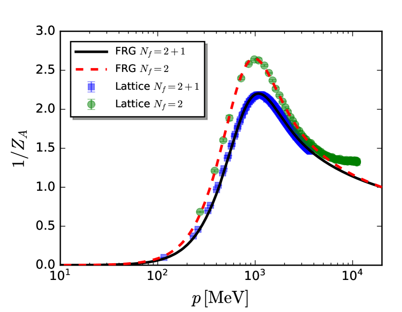
Figure 25: $N_{f}=2$ flavour and $N_{f}=2+1$ gluon dressing functions $1/Z_{A}$ as function of momentum. The $N_{f}=2$ flavour gluon dressing computed with the fRG in Cyrol et al. (2018a) is the input in the present work. It is in quantitative agreement with the respective lattice results. The lattice data here are taken from Sternbeck et al. (2012). The $N_{f}=2+1$ flavour gluon dressing shown here is a genuine prediction of the present computation. It is shown to be in quantitative agreement with the respective lattice results Zafeiropoulos et al. (2019); Boucaud et al. (2018, 2019).

This completes our scale setting for the physical point. All quantities are measured in the respective absolute units.

For the sake of completeness we also provide results for the pion decay constant. This computation is also interesting in terms of the predictive power as well as the limitations of the present approximation. The pion decay constant can be determined from the momentum dependence of the quark propagator dressings $Z_{q}(p)$ and $M_{q}(p)$, defined in (77). These dressings are linked to the Bethe-Salpether wave function of the pion, for reviews see e.g. Fischer (2006); Bashir et al. (2012); Eichmann et al. (2016b),

$$f^{2}_{\pi}=\frac{3}{2\pi^{2}}\int_{0}^{\infty}dp\,\frac{p^{3}\,M_{q}(p)}{\left[p^{2}+M_{q}(p)\right]^{2}}\left[M_{q}(p)-p\frac{\partial M_{q}(p)}{\partial p}\right]\,.$$ (191)

Equation (191) is sensitive to the full momentum dependence of the quark mass function $M_{q}(p)$. This dependence is suppressed in the flows due to the presence of the regulator term in the propagators. The letter suppression is the argument for the momentum-independent approximation in the present work with $m_{l,k}=M_{q,k}(p=0)$. Note also that the results in Cyrol et al. (2018a) have been obtained for a fixed expansion point or background with $\partial_{t}\kappa=0$ with a four-dimensional flat regulator. Both properties can be taken account in the present work by evaluating the mass function on a fixed background $\kappa=1/2\sigma_{\textrm{EoM}}$ at vanishing cutoff $k=0$ as well as rescaling the cutoff scale $k\to 3/4k$. Moreover, we have to rescale the mass function $M_{q,k}\to M_{q,k}m_{l,0}/M_{q,0}$ in order to have the same infrared value. This leads us to Figure 26, which first of all confirms impressively the validity of our approximation scheme.

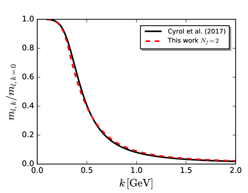
Figure 26: Two-flavour QCD quark mass functions from Cyrol et al. (2018a) and the present work for a fixed background $\sigma=\sigma_{\textrm{EoM}}$ at vanishing cutoff scale. In Cyrol et al. (2018a) the full momentum-dependent mass $M_{q,k}(p)$ function in $N_{f}=2$ flavour QCD has been computed, and we have $m_{l.k}/m_{l.k=0}=M_{q,k}(0)/M_{q,k=0}(0)$.

Moreover it allows us to use the rescaled quark mass function $M_{q,\textrm{res}}(p)$ of Cyrol et al. (2018a) for an estimate of $f_{\pi}$ in the present work with (191). The rescaled quark mass function reads

$$M_{q,\textrm{res}}(p)=M_{q,k=0}(p)\frac{m_{l,k=0}}{M_{q,k=0}(0)}\,,$$ (192)

and the result for the pion decay constant at the physical point is

$$f_{\pi}\approx 96.0\,\textrm{MeV}\,,$$ (193)

see also Table 1. In the current approximation the $N_{f}=2+1$ flavour mass function has the same cutoff behaviour as the $N_{f}=2$ flavour one. This is related to the fact, that the strange quark feeds into the light quark mass function only indirectly over the gluon propagator and running coupling $\alpha_{\bar{l}Al}$ in the quark-gluon vertex. Rescaling the mass functions with their value at $k=0$ makes this very apparent, see Figure 27.

We conclude that the agreement of the rescaled $M_{q,k}(0)$ with the $N_{f}=2+1$ flavour light quark mass function $m_{l,k}$ works equally well as for the two-flavour case depicted in Figure 26. The respective plot is shown in Figure 28.

Consequently we can use the same estimate as in (192) for the $N_{f}=2+1$ flavour case. This leads us to

$$f_{\pi}\approx 93.0\,\textrm{MeV}\,,$$ (194)

see also Table 1. Finally we are interested in the pion decay constant in the chiral limit. The respective light quark mass function $m_{l,\chi}$ at $k=0$ is given by $m_{l,\chi}=319$  MeV, leading to

$$f_{\pi,\chi}\approx 88.6\,\textrm{MeV}$$ (195)

In summary the scale setting in the present work is selfconsistent with both the confinement scales, here determined via the gluon dressing function, as well as the chiral symmetry breaking ones, here determined with the pion decay constant. This is further nontrivial evidence for the reliability of the present approximation for not too large chemical potential.

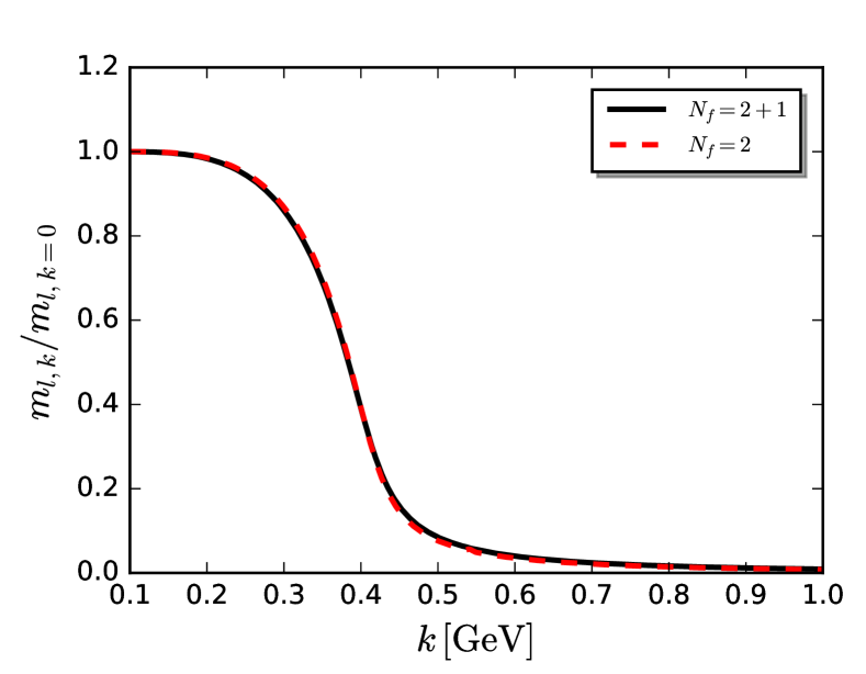
Figure 27: $N_{f}=2$ and $N_{f}=2+1$ light quark mass functions as a function of the cutoff scale $k$, normalised by their value at vanishing cutoff scale $k=0$.

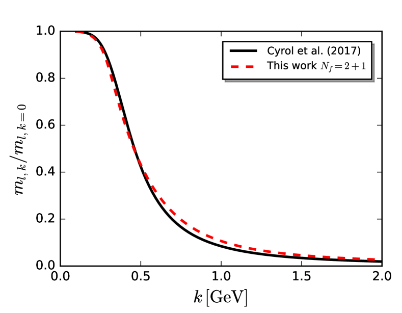
Figure 28: $N_{f}=2$ quark mass function from Cyrol et al. (2018a) and the $N_{f}=2+1$ light quark mass function from present work in the fixed expansion.

Appendix F Flow of the effective potential

Within the approximation discussed in Section IV.4, the effective potential $V_{\mathrm{mat},k}(\rho,L,\bar{L})$ in (40) satisfies the flow equation (26), which we recall,

$$\partial_{t}V_{\mathrm{mat},k}(\rho) =\frac{k^{4}}{4\pi^{2}}\big{[}(N_{f}^{2}-1)l_{0}^{(B,4)}(\tilde{m}_{\pi,k}^{2},\eta_{\phi,k};T)$$

$$\quad+l_{0}^{(B,4)}(\tilde{m}_{\sigma,k}^{2},\eta_{\phi,k};T)$$

$$\quad-4N_{c}N_{f}l_{0}^{(F,4)}(\tilde{m}_{q,k}^{2},\eta_{q,k};T,\mu_{q})\big{]}\,,$$ (196)

where the threshold functions $l_{0}^{(B/F,4)}$ are given in (233) and (234) in Appendix N, and the Polyakov loops $L,\bar{L}$ are not shown explicitly for brevity. The right hand side of (196) also depends on the dimensionless renormalised quark and meson masses, i.e.,

$$\tilde{m}_{q,k}^{2} =\frac{h_{k}^{2}\rho}{2k^{2}Z_{q,k}^{2}}\,,\quad\quad\tilde{m}_{\pi,k}^{2}=\frac{V_{k}^{\prime}(\rho)}{k^{2}\bar{Z}_{\phi,k}}\,,$$

$$\tilde{m}_{\sigma,k}^{2} =\frac{V_{k}^{\prime}(\rho)+2\rho V_{k}^{\prime\prime}(\rho)}{k^{2}\bar{Z}_{\phi,k}}\,.$$ (197)

Performing a Taylor expansion of the effective potential, one arrives at

$$V_{\mathrm{mat},k}(\rho) =\sum_{n=0}^{N_{v}}\frac{\lambda_{n,k}}{n!}(\rho-\kappa_{k})^{n}\,,$$ (198)

where the expansion point $\kappa_{k}$ can depend on the RG scale. Note that the expansion coefficients $\lambda_{n,k}$ should not be confused with the four-fermion coupling $\lambda_{q}$ in (39). It is more convenient to work with RG-invariant variables, which are denoted in this paper by quantities with a bar, except for the strong couplings in (54) and (55), for example, $\bar{\rho}=\bar{Z}_{\phi,k}\rho$, $\bar{\kappa}_{k}=\bar{Z}_{\phi,k}\kappa_{k}$, and $\bar{\lambda}_{n,k}=\lambda_{n,k}/\bar{Z}_{\phi,k}^{n}$ with $\bar{Z}_{\phi}$ defined in (92). The $\eta^{\ }_{\Phi_{i},k}$’s in (196) are the anomalous dimensions for respective fields, which are given in (30). We reformulate the effective potential in terms of RG-invariant variables through $V_{\mathrm{mat},k}(\rho)=\bar{V}_{\mathrm{mat},k}(\bar{\rho})$, i.e.,

$$\bar{V}_{\mathrm{mat},k}(\bar{\rho}) =\sum_{n=0}^{N_{v}}\frac{\bar{\lambda}_{n,k}}{n!}(\bar{\rho}-\bar{\kappa}_{k})^{n}\,.$$ (199)

The expansion point $\bar{\kappa}_{k}$ can be chosen freely, provided that the physics of our concern is within the radius of convergence of the expansion Pawlowski and Rennecke (2014). Expanding about a fixed background is a convenient choice, see e.g. Pawlowski and Rennecke (2014); Braun et al. (2016a); Fu and Pawlowski (2015); Rennecke and Schaefer (2017), where the unrenormalised expansion point is chosen to be independent of $k$. In this work we adopt the physical point expansion. In this expansion $\bar{\kappa}_{k}$ is chosen to be the minimum of the effective potential at each scale $k$, i.e. it is given by the solution of the EoM,

$$\frac{\partial}{\partial\bar{\rho}}\Big{(}\bar{V}_{k}(\bar{\rho})-\bar{c}_{k}\bar{\sigma}\Big{)}\bigg{|}_{\bar{\rho}=\bar{\kappa}_{k}} =0\,.$$ (200)

With (196) and (200), see also (159), one obtains the flow of the expansion point in (199), to wit,

$$\partial_{t}\bar{\kappa}_{k}= -\frac{\bar{c}_{k}^{2}}{\bar{\lambda}_{1,k}^{3}+\bar{c}_{k}^{2}\bar{\lambda}_{2,k}}\bigg{[}\eta_{\phi,k}\Big{(}\frac{\bar{\lambda}_{1,k}}{2}+\bar{\kappa}_{k}\bar{\lambda}_{2,k}\Big{)}$$

$$+\left.\partial_{\bar{\rho}}\partial_{t}\big{|}_{\rho}\bar{V}_{k}(\bar{\rho})\big{)}\right|_{\bar{\rho}=\bar{\kappa}_{k}}\bigg{]}\,.$$ (201)

The flow equations of the expansion coefficients of the effective potential $\bar{\lambda}_{n,k}$, which describe $2n$-meson scattering, are

$$\partial_{t}\bar{\lambda}_{n,k}= \partial_{\bar{\rho}}^{n}\big{(}\partial_{t}\big{|}_{\rho}\bar{V}_{k}(\bar{\rho})\big{)}\Big{|}_{\bar{\rho}=\bar{\kappa}_{k}}+n\eta_{\phi,k}\bar{\lambda}_{n,k}$$

$$+\big{(}\partial_{t}\bar{\kappa}_{k}+\eta_{\phi,k}\bar{\kappa}_{k}\big{)}\bar{\lambda}_{n+1,k}\,.$$ (202)

In this work the maximal order of the Taylor expansion for the effective potential in (199) is chosen to be $N_{v}=5$, and we have checked its convergence for the $\mu_{B}$-range studied here, $0\leq\mu_{B}\lesssim 600$ MeV.

Appendix G Glue potential

We employ the parameterisation put forward in Lo et al. (2013) for the glue potential in (69). The advantage is that, besides the expectation value of the Polyakov loop and the pressure in Yang-Mills theory, quadratic fluctuations of the Polyakov loop are taken into account. For a detailed discussion we refer to Fu and Pawlowski (2015). The glue potential reads

$$V_{\text{glue}}(L,\bar{L}) =-\frac{a(T)}{2}\bar{L}L+b(T)\ln M_{H}(L,\bar{L})$$

$$\quad+\frac{c(T)}{2}(L^{3}+\bar{L}^{3})+d(T)(\bar{L}L)^{2}\,,$$ (203)

with the Haar measure

$$M_{H}(L,\bar{L}) =1-6\bar{L}L+4(L^{3}+\bar{L}^{3})-3(\bar{L}L)^{2}\,.$$ (204)

The temperature dependence of coefficients on the r.h.s. of (203) enters through

$$x(T) =\frac{x_{1}+x_{2}/(t_{\text{\tiny{YM}}}+1)+x_{3}/(t_{\text{\tiny{YM}}}+1)^{2}}{1+x_{4}/(t_{\text{\tiny{YM}}}+1)+x_{5}/(t_{\text{\tiny{YM}}}+1)^{2}}\,,$$ (205)

for $x\in\{a,c,d\}$, and

$$b(T) =b_{1}(t_{\text{\tiny{YM}}}+1)^{-b_{4}}\left(1-e^{b_{2}/(t_{\text{\tiny{YM}}}+1)^{b_{3}}}\right)\,.$$ (206)

The constants in 205 and 206 are taken from Lo et al. (2013), and are also collected in Table 3 for convenience. $t_{\text{\tiny{YM}}}$ is related to the reduced temperature of Yang-Mills theory, and it has been found in Pawlowski (2011); Haas et al. (2013); Herbst et al. (2014) that unquenching effects in QCD are well captured through a linear rescaling of the reduced temperature of the pure gauge theory,

$$t_{\text{\tiny{YM}}} \rightarrow\alpha\,t_{\text{\tiny{glue}}}\quad\text{with}\quad t_{\text{\tiny{glue}}}=(T-T_{c}^{\text{\tiny{glue}}})/T_{c}^{\text{\tiny{glue}}},$$ (207)

where $\alpha=0.57$, $T_{c}^{\text{\tiny{glue}}}$=250 MeV for $N_{f}=2$ and 225 MeV for $N_{f}=2+1$ are used in this work. For more relevant details, see the foregoing references.

	1	2	3	4	5
$a_{i}$	-44.14	151.4	-90.0677	2.77173	3.56403
$b_{i}$	-0.32665	-82.9823	3.0	5.85559
$c_{i}$	-50.7961	114.038	-89.4596	3.08718	6.72812
$d_{i}$	27.0885	-56.0859	71.2225	2.9715	6.61433

Table 3: Constants in (205) and (206) for the glue potential.

Appendix H Gluon anomalous dimension

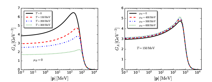
Figure 29: $N_{f}=2+1$ gluon propagator $G_{A}=1/(Z_{A,k}k^{2})$ at vanishing frequency $p_{0}=0$ as a function of spatial momenta $|\bm{p}|$ at different temperatures (left panel) and baryon chemical potentials (right panel).

Implementing the projection as shown in (104), one obtains the contribution of the quark loop to the gluon anomalous dimension, which reads

$$\eta_{A}^{q} =-\frac{N_{f}}{\pi^{2}}g_{\bar{q}Aq,k}^{2}\int_{0}^{1}dx\bigg{[}(1-\eta_{q,k})\sqrt{x}+\eta_{q,k}x\bigg{]}$$

$$\times\int_{-1}^{1}d\cos\theta\bigg{[}\Big{(}\mathcal{FF}_{(1,1)}(\tilde{m}_{q,k}^{2},\tilde{m}_{q,k}^{2})$$

$$-\mathcal{FF}_{(2,1)}(\tilde{m}_{q,k}^{2},\tilde{m}_{q,k}^{2})\Big{)}+\Big{(}\sqrt{x}\cos^{2}\!\theta-\cos\theta\Big{)}$$

$$\times\Big{(}1+r_{F}(x^{\prime})\Big{)}\Big{(}\mathcal{FF}_{(2,1)}(\tilde{m}_{q,k}^{2},\tilde{m}_{q,k}^{2})$$

$$-\frac{1}{2}\mathcal{FF}_{(1,1)}(\tilde{m}_{q,k}^{2},\tilde{m}_{q,k}^{2})\Big{)}\bigg{]}\,,$$ (208)

with the fermionic regulator in (225d). We have defined $x=\bm{q}^{2}/k^{2}$, $x^{\prime}=(\bm{q}-\bm{p})^{2}/k^{2}$. $\bm{q}$ and $\bm{p}$ are the loop and external momenta, respectively, and $\theta$ is the angle between them. In order to take into account the screening effect of the quark on the gluon propagator more efficiently, we choose the external momentum to be $|\bm{p}|=k$ in (208). This is necessary for consistence, since we also evaluate the external input for the gluon anomalous dimension at $|\bm{p}|=k$. The in-medium contribution, which we use for the light-quark contribution, is then

$$\Delta\eta_{A}^{q}=\eta_{A}^{q}-\eta_{A}^{q}\big{|}_{T,\mu=0}\,.$$ (209)

The threshold functions in (208) are given in (244). Moreover, the second term on the r.h.s. of (100), viz. $\Delta\eta_{A}^{\text{glue}}$, which is the thermal part of the pure glue contribution to the gluon anomalous dimension, has to be specified. Again, we build on the results in Yang-Mills theory in Cyrol et al. (2018b). As discussed there, $\Delta\eta_{A}^{\text{glue}}$ is captured quantitatively through the inclusion of a thermal screening mass of the gluon, $\Delta m_{\textrm{scr}}^{2}(k,T)$. In addition to the temperature, it has to depend on the RG scale since thermal effects are rapidly suppressed for $k\gtrsim 2\pi T$. Therefore, in the following we discuss the modification of the gluon anomalous dimension resulting from its thermal screening mass. Beginning with the inverse gluon propagator,

$$G_{A}^{-1}(k) =Z_{A,k}k^{2}\,,$$ (210)

one obtains a modified one with the screening mass,

$$\bar{G}_{A}^{-1}(k) =\bar{Z}_{A,k}k^{2}=Z_{A,k}k^{2}+\Delta m_{\textrm{scr}}^{2}(k,T)\,.$$ (211)

Differentiating both sides with respect to $t$ leads to

$$\bar{Z}_{A,k}k^{2}(2-\bar{\eta}_{A,k}) =Z_{A,k}k^{2}(2-\eta_{A,k})+\partial_{t}\big{(}\Delta m_{\textrm{scr}}^{2}(k,T)\big{)}\,.$$ (212)

where $\bar{\eta}_{A}=-\partial_{t}\bar{Z}_{A}/\bar{Z}_{A}$ is the anomalous dimension with the screening mass. Replacing $Z_{A}$ in (212) by resorting to (211), one is led to

$$\bar{\eta}_{A} =\eta_{A}+\frac{\Delta m_{\textrm{scr}}^{2}(k,T)}{\bar{Z}_{A}k^{2}}(2-\eta_{A})$$

$$-\frac{1}{\bar{Z}_{A}k^{2}}\partial_{t}\big{(}\Delta m_{\textrm{scr}}^{2}(k,T)\big{)}\,.$$ (213)

Guided by the results of Cyrol et al. (2018b), we propose an ansatz for the screening mass as follows:

$$\Delta m_{\textrm{scr}}^{2}(k,T) =(c\,T)^{2}\exp\Big{[}-\Big{(}\frac{k}{\pi T}\Big{)}^{n}\Big{]}\,.$$ (214)

Here $c=2$ is adopted for $N_{f}=2+1$, which is consistent with the result in Cyrol et al. (2018b). Furthermore, we choose $n=2$ in (214). We have also investigated the dependence of our results on the parameters in (214), and find that variations of the parameters result in only a mild change of the pseudocritical temperature of the chiral phase transition.

In Section V.3 we show the momentum (or cutoff) dependence of the gluon dressing function $1/Z_{A}(p)$ for different temperatures and baryon chemical potentials. In particular the dependence on $\mu_{B}$ is very mild and only concerns the infrared. The in-medium behaviour is more pronounced in the gluon propagator depicted in Figure 29. However, we emphasise that the dressing functions are the relevant quantities for the flow equations in the present work.

Appendix I Scalar anomalous dimension

The anomalous dimensions of the mesons for vanishing external momentum $p=0$ and nonvanishing momentum $(p_{0}=0,|\bm{p}|=k)$ are given by (96) and (93), respectively. This leads us to

$$\eta_{\phi}(0)= \,\frac{\bar{Z}_{\phi}}{Z_{\phi}(0)}$$

$$\,\times\frac{1}{6\pi^{2}}\bigg{\{}\frac{4}{k^{2}}\bar{\kappa}_{k}(\bar{V}^{{}^{\prime\prime}}_{k}(\bar{\kappa}_{k}))^{2}\mathcal{BB}_{(2,2)}(\tilde{m}_{\pi,k}^{2},\tilde{m}_{\sigma,k}^{2};T)$$

$$\,+N_{c}\bar{h}_{k}^{2}\Big{[}(2\eta_{q,k}-3)\mathcal{F}_{(2)}(\tilde{m}_{q,k}^{2};T,\mu_{q})$$

$$\,-4(\eta_{q,k}-2)\mathcal{F}_{(3)}(\tilde{m}_{q,k}^{2};T,\mu_{q})\Big{]}\bigg{\}}\,,$$ (215)

where the ratio $\bar{Z}_{\phi}/Z_{\phi}(0)$ takes into account that the flow on the right hand side of (215) has been defined with derivatives w.r.t. the renormalised field $\bar{\phi}=\bar{Z}_{\phi}\phi$. The term with the threshold function $\mathcal{BB}_{(2,2)}$ arises from the mesonic loop of the flow equation for the meson propagator in Figure 5. The terms involving $\mathcal{F}_{(n)}$ are related to the quark loop. Explicit expressions for all threshold functions are collected in Appendix N. For (93) we have with $(0,k)=(p_{0}=0,|\mathbf{p}|=k)$,

$$\eta_{\phi}(0,k)$$

$$= \frac{2}{3\pi^{2}}\frac{1}{k^{2}}\bar{\kappa}_{k}(\bar{V}^{{}^{\prime\prime}}_{k}(\bar{\kappa}_{k}))^{2}\mathcal{BB}_{(2,2)}(\tilde{m}_{\pi,k}^{2},\tilde{m}_{\sigma,k}^{2};T)$$

$$-\frac{N_{c}}{\pi^{2}}\bar{h}_{k}^{2}\int_{0}^{1}dx\bigg{[}(1-\eta_{q,k})\sqrt{x}+\eta_{q,k}x\bigg{]}$$

$$\times\int_{-1}^{1}d\cos\theta\Bigg{\{}\bigg{[}\Big{(}\mathcal{FF}_{(1,1)}(\tilde{m}_{q,k}^{2},\tilde{m}_{q,k}^{2})-\mathcal{F}_{(2)}(\tilde{m}_{q,k}^{2})\Big{)}$$

$$-\Big{(}\mathcal{FF}_{(2,1)}(\tilde{m}_{q,k}^{2},\tilde{m}_{q,k}^{2})-\mathcal{F}_{(3)}(\tilde{m}_{q,k}^{2})\Big{)}\bigg{]}$$

$$+\bigg{[}\Big{(}\sqrt{x}-\cos\theta\Big{)}\Big{(}1+r_{F}(x^{\prime})\Big{)}\mathcal{FF}_{(2,1)}(\tilde{m}_{q,k}^{2},\tilde{m}_{q,k}^{2})$$

$$-\mathcal{F}_{(3)}(\tilde{m}_{q,k}^{2})\bigg{]}-\frac{1}{2}\bigg{[}\Big{(}\sqrt{x}-\cos\theta\Big{)}\Big{(}1+r_{F}(x^{\prime})\Big{)}$$

$$\times\mathcal{FF}_{(1,1)}(\tilde{m}_{q,k}^{2},\tilde{m}_{q,k}^{2})-\mathcal{F}_{(2)}(\tilde{m}_{q,k}^{2})\bigg{]}\Bigg{\}}\,,$$ (216)

with $x=\bm{q}^{2}/k^{2}$ and $x^{\prime}=(\bm{q}-\bm{p})^{2}/k^{2}$ as same as in (208). Note that in (216) we have neglected the external momentum dependence of the meson loop for simplicity in the numerical calculations. This is a good approximation for both, small and large $k$, since meson loops are suppressed by the meson masses in the IR and decouple in the UV. Only in the phase transition region and in particular at the CEP, corrections to the mesonic part of (216) could become relevant.

Appendix J Quark anomalous dimension

The quark anomalous dimension $\eta_{q,k}$ in (80) reads

$$\eta_{q,k}= \frac{1}{24\pi^{2}N_{f}}(4-\eta_{\phi,k})\bar{h}_{k}^{2}$$

$$\times\bigg{\{}(N_{f}^{2}-1)\mathcal{FB}_{(1,2)}(\tilde{m}_{q,k}^{2},\tilde{m}_{\pi,k}^{2};T,\mu_{q},p_{0,\text{\tiny{ex}}})$$

$$+\mathcal{FB}_{(1,2)}(\tilde{m}_{q,k}^{2},\tilde{m}_{\sigma,k}^{2};T,\mu_{q},p_{0,\text{\tiny{ex}}})\bigg{\}}$$

$$+\frac{1}{24\pi^{2}}\frac{N_{c}^{2}-1}{2N_{c}}g_{\bar{q}Aq,k}^{2}$$

$$\times\bigg{\{}2(4-\eta_{A,k})\mathcal{FB}_{(1,2)}(\tilde{m}_{q,k}^{2},0;T,\mu_{q},p_{0,\text{\tiny{ex}}})$$

$$+3(3-\eta_{q,k})\Big{(}\mathcal{FB}_{(1,1)}(\tilde{m}_{q,k}^{2},0;T,\mu_{q},p_{0,\text{\tiny{ex}}})$$

$$-2\mathcal{FB}_{(2,1)}(\tilde{m}_{q,k}^{2},0;T,\mu_{q},p_{0,\text{\tiny{ex}}})\Big{)}\bigg{\}},$$ (217)

where the fermion-boson mixed threshold function $\mathcal{FB}$’s are given in Appendix N. It is obvious that the contributions in (217) can be divided into two sectors, which results from the quark-meson and quark-gluon interactions, respectively.

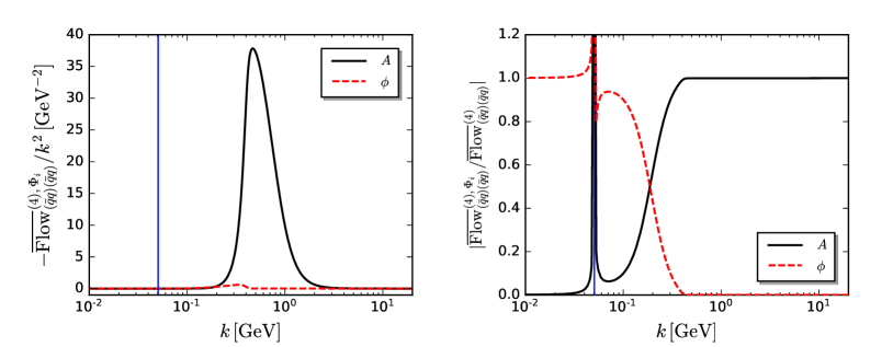
Figure 30: Left panel: comparison between the flow of the $N_{f}=2+1$ four–light-quark coupling arising from the gluon exchange in (220), $\Phi_{i}=A$, and that from the meson exchange in (221), $\Phi_{i}=\phi$, as a function of $k$ at $T=\mu_{B}=0$.
Right panel: the ratio of their respective flow over the total flow, i.e., the summation of (220) and (221), where the absolute value for the ratio is chosen. The blue vertical line in both plots shows the position where the flow resulting from the meson exchange changes sign.

The external 3-momentum in (217) is chosen to be $\bm{p}=0$. However, since the fermionic Matsubara frequency, $p_{0}=(2n+1)\pi T$ with $n\in\mathbb{Z}$, does not have a zero-mode, $p_{0}$ cannot be chosen to be zero. In fact, a truncation that takes into account the full frequency dependence of the quark anomalous dimension plays a significant r$\hat{\textrm{o}}$le in obtaining quantitative accuracy in the computation of particle number correlations with the fRG, and is also indispensable to guarantee the Silver Blaze properties at finite chemical potential, see Fu et al. (2016) for more relevant details. However, a frequency dependent truncation is computationally very demanding, in particular in a temporal gluon background field. Hence, in the present work we use a modification of the lowest Matsubara mode. As has been discussed in detail in Fu and Pawlowski (2015), an evaluation consistent with the silver blaze property is done with

$$p_{0,\text{\tiny{ex}}}=(\pi T)\exp\{-k/(\pi T)\}-i\,\mu_{q}\,.$$ (218)

We use the exponential factor to suppress the artificial $T$-dependence in the vacuum part of the flow that is introduced by the fermionic Matsubara frequency. As discussed in Fu and Pawlowski (2015); Fu et al. (2016), this procedure is necessary to ensure the correct thermal behaviour without taking into account the full frequency dependence. The chemical potential part eliminates the $\mu$-part of the argument $p_{0}+i\,\mu_{q}$ of the correlation functions. This keeps the expansion point $p_{0,\text{\tiny{ex}}}+i\,\mu_{q}$ fixed and does not lead to an unphysical $\mu_{q}$-dependence. The even quantitative reliability of this treatment has been verified in Fu et al. (2016) through a comparison with the fully frequency-dependent calculations.

In comparison to Fu and Pawlowski (2015) we use the limit $p_{0,\text{\tiny{ex}}}+i\,\mu_{q}\to 0$ instead of $p_{0,\text{\tiny{ex}}}+i\,\mu_{q}\to k$ for convenience. This modification allows us to compare our vacuum results more directly to that in Braun et al. (2016a), as there the flows are evaluated at $p_{0,\text{\tiny{ex}}}=0$. We drop the suppression factor in the thermal part of the diagrams: $p_{0,\text{\tiny{ex}}}\to(\pi T)-i\,\mu_{q}$. This leads to simpler expressions, and the necessary suppression of thermal effects at small $T/k$ is guaranteed by the thermal distribution functions. Both modifications have no sizable impact on the numerical results.

Appendix K Flow of the Yukawa coupling

We have discussed the Yukawa coupling in Section IV.3, and its flow is given in (115). Adopting the same external frequency and momentum as the quark anomalous dimension, the last term on the r.h.s. of (115) reads

$$\mathrm{Re}\big{(}\overline{\textrm{Flow}}^{(2)}_{(\bar{q}\tau^{0}q)}\big{)}/\bar{\sigma}$$

$$\quad=\frac{1}{4\pi^{2}N_{f}}\bar{h}_{k}^{3}\bigg{[}-(N_{f}^{2}-1)$$

$$\qquad\times L_{(1,1)}^{(4)}(\tilde{m}_{q,k}^{2},\tilde{m}_{\pi,k}^{2},\eta_{q,k},\eta_{\phi,k};T,\mu_{q},p_{0,\text{\tiny{ex}}})$$

$$\qquad+L_{(1,1)}^{(4)}(\tilde{m}_{q,k}^{2},\tilde{m}_{\sigma,k}^{2},\eta_{q,k},\eta_{\phi,k};T,\mu_{q},p_{0,\text{\tiny{ex}}})\bigg{]}$$

$$\qquad-\frac{3}{2\pi^{2}}\frac{N_{c}^{2}-1}{2N_{c}}g_{\bar{q}Aq,k}^{2}\bar{h}_{k}$$

$$\qquad\times L_{(1,1)}^{(4)}(\tilde{m}_{q,k}^{2},0,\eta_{q,k},\eta_{A,k};T,\mu_{q},p_{0,\text{\tiny{ex}}})\,.$$ (219)

Appendix L Flow of the four-quark coupling

The flow diagrams of the four-quark coupling arising from the gluon exchange in the first line in Figure 4, after projected onto the $\sigma$-$\bm{\pi}$ channel, are denoted with $\overline{\textrm{Flow}}^{(4),A}_{(\bar{q}q)(\bar{q}q)}$. The flow diagrams arising from the meson exchange or denoted with $\overline{\textrm{Flow}}^{(4),\phi}_{(\bar{q}q)(\bar{q}q)}$. The gluon exchange diagrams read

$$\overline{\textrm{Flow}}^{(4),A}_{(\bar{q}q)(\bar{q}q)} =-\frac{3}{2\pi^{2}}\frac{N_{c}^{2}-1}{2N_{c}}\Big{(}\frac{3}{4}-\frac{1}{N_{c}^{2}}\Big{)}g_{\bar{q}Aq,k}^{4}$$

$$\quad\times\bigg{\{}\frac{2}{15}(5-\eta_{A,k})\Big{[}\mathcal{FB}_{(1,3)}(\tilde{m}_{q,k}^{2},0)$$

$$\quad-\bar{m}_{q,k}^{2}\mathcal{FB}_{(2,3)}(\tilde{m}_{q,k}^{2},0)\Big{]}$$

$$\quad+\frac{1}{12}(4-\eta_{q,k})\Big{[}\mathcal{FB}_{(2,2)}(\tilde{m}_{q,k}^{2},0)$$

$$\quad-2\bar{m}_{q,k}^{2}\mathcal{FB}_{(3,2)}(\tilde{m}_{q,k}^{2},0)\Big{]}\,,$$ (220)

Here, the arguments $T$, $\mu_{q}$ and $p_{0,\text{\tiny{ex}}}$ for threshold functions are not shown explicitly. The right hand side of (220) is obtained as follows: It contains expressions such as $(q\cdot q^{F})(\gamma\cdot q)(\gamma\cdot q^{F})/q^{2}$ with loop momentum $q$. Here, $q_{\mu}^{F}\equiv(q_{0},(1+r_{F})\bm{q})$ with $r_{F}$ in (225a). This expression arises from the quark propagator with the 3$d$ regulator as shown in Eq. (225a), contracted with the transverse magnetic tensor of the gluon in Eq. (105). In order to simplify the flow in Eq. (220) as well as numerical calculations, we approximate the expression above as $q^{F}\cdot q^{F}$, which is exact for the 4$d$ regulator. We have also investigated the reliability of this approximation through the comparison to the relevant four-quark flow in Braun et al. (2016a). There a 4$d$ regulator has been used, and we find that the difference is negligible.

The meson exchange diagrams have the form

$$\overline{\textrm{Flow}}^{(4),\phi}_{(\bar{q}q)(\bar{q}q)} =\frac{1}{32\pi^{2}}\frac{N_{f}^{2}-2}{N_{f}N_{c}}\bar{h}_{k}^{4}\bigg{\{}\frac{2}{15}(5-\eta_{\phi,k})$$

$$\quad\times\Big{[}\Big{(}\mathcal{FBB}_{(1,1,2)}(\tilde{m}_{q,k}^{2},\tilde{m}_{\pi,k}^{2},\tilde{m}_{\sigma,k}^{2})$$

$$\quad+\mathcal{FBB}_{(1,1,2)}(\tilde{m}_{q,k}^{2},\tilde{m}_{\sigma,k}^{2},\tilde{m}_{\pi,k}^{2})$$

$$\quad-2\mathcal{FB}_{(1,3)}(\tilde{m}_{q,k}^{2},\tilde{m}_{\pi,k}^{2})\Big{)}$$

$$\quad-\tilde{m}_{q,k}^{2}\Big{(}\mathcal{FBB}_{(2,1,2)}(\tilde{m}_{q,k}^{2},\tilde{m}_{\pi,k}^{2},\tilde{m}_{\sigma,k}^{2})$$

$$\quad+\mathcal{FBB}_{(2,2,1)}(\tilde{m}_{q,k}^{2},\tilde{m}_{\pi,k}^{2},\tilde{m}_{\sigma,k}^{2})$$

$$\quad-2\mathcal{FB}_{(2,3)}(\tilde{m}_{q,k}^{2},\tilde{m}_{\pi,k}^{2})\Big{)}\Big{]}+\frac{1}{6}(4-\eta_{q,k})$$

$$\quad\times\Big{[}\Big{(}\mathcal{FBB}_{(2,1,1)}(\tilde{m}_{q,k}^{2},\tilde{m}_{\pi,k}^{2},\tilde{m}_{\sigma,k}^{2})$$

$$\quad-\mathcal{FB}_{(2,2)}(\tilde{m}_{q,k}^{2},\tilde{m}_{\pi,k}^{2})\Big{)}$$

$$\quad-2\tilde{m}_{q,k}^{2}\Big{(}\mathcal{FBB}_{(3,1,1)}(\tilde{m}_{q,k}^{2},\tilde{m}_{\pi,k}^{2},\tilde{m}_{\sigma,k}^{2})$$

$$\quad-\mathcal{FB}_{(3,2)}(\tilde{m}_{q,k}^{2},\tilde{m}_{\pi,k}^{2})\Big{)}\Big{]}\bigg{\}}\,.$$ (221)

In Figure 30 we compare (220) and (221) at $T=0$ and $\mu_{B}=0$ for the purpose of illustration. The flow divided by $k^{2}$ is shown in the left plot of Figure 30, and the ratio between the respective flow and their sum in the right plot. Note that the peak in the right plot corresponds to the position where the sum of (220) and (221) is vanishing, thus resulting in a divergent ratio there. This is because in the low $k$ region meson exchange dominates, and this contribution changes sign at about $k\approx 75$ MeV, as shown by the blue vertical line in both plots. One observes that gluon exchange, i.e., the diagrams in the first line in Figure 4, is the dominant process for $k\gtrsim 300$ MeV. Therefore, it is reasonable to expect that the mixed diagrams in the third line of Figure 4 play a subleading r$\hat{\textrm{o}}$le for dynamical hadronisation. It is interesting to observe that gluon exchange becomes dominant already in (and below) the phase transition region at $k\approx 400$ MeV, which can be read-off, e.g., from Figure 8. This gives an implicit upper bound on the validity of low-energy models, namely $k\lesssim 300$ MeV. For first discussions in this direction, see Rennecke (2015b); Alkofer et al. (2019). Note that this bound is in quantitative agreement with the results in these references.

Appendix M Flow of the quark-gluon coupling

The running of the strong quark-gluon coupling is governed by (106), where the term in the second line is divided into two parts, i.e., $\overline{\textrm{Flow}}^{(3),A}_{(\bar{q}Aq)}$ and $\overline{\textrm{Flow}}^{(3),\phi}_{{(\bar{q}Aq)}}$, which correspond to the relevant contributions from the quark-gluon and quark-meson couplings, respectively. The subscript ${}_{{(\bar{q}Aq)}}$ indicates that these expressions are the projections of the quark-gluon flows on the running coupling, see (106). With this notation, the flow of the light-quark–gluon coupling is:

$$\partial_{t}g_{\bar{l}Al} =\left(\frac{1}{2}\eta_{A}+\eta_{q}\right)g_{\bar{l}Al}$$

$$\quad+\bigg{(}N_{f}\,\overline{\textrm{Flow}}^{(3),A}_{(\bar{l}Al)}+\overline{\textrm{Flow}}^{(3),\phi}_{{(\bar{q}Aq)}}\bigg{)}\bigg{|}_{N_{f}=2}\,.$$ (222)

The explicit form of the flow of the strange-quark–gluon coupling is given in (175). The gluonic contribution reads

$$\overline{\textrm{Flow}}^{(3),A}_{(\bar{q}Aq)}= \frac{3}{8\pi^{2}N_{c}}g_{\bar{q}Aq}^{3}\tilde{m}_{q,k}^{2}\bigg{\{}\frac{2}{15}(5-\eta_{A,k})\mathcal{FB}_{(2,2)}(\tilde{m}_{q,k}^{2},0)$$

$$+\frac{1}{3}(4-\eta_{q,k})\mathcal{FB}_{(3,1)}(\tilde{m}_{q,k}^{2},0)\bigg{\}}$$

$$+\frac{3N_{c}}{8\pi^{2}}g_{\bar{q}Aq}^{2}g_{A^{3}}\bigg{\{}\frac{1}{20}(5-\eta_{q,k})\mathcal{FB}_{(1,2)}(\tilde{m}_{q,k}^{2},0)$$

$$-\frac{1}{6}(4-\eta_{q,k})\mathcal{FB}_{(2,1)}(\tilde{m}_{q,k}^{2},0)+\frac{1}{30}(5-2\eta_{q,k})$$

$$\times\mathcal{FB}_{(2,2)}(\tilde{m}_{q,k}^{2},0)-\frac{4}{15}(5-\eta_{A,k})$$

$$\times\mathcal{FB}_{(1,2)}(\tilde{m}_{q,k}^{2},0)+\frac{1}{30}(10-3\eta_{A,k})$$

$$\times\mathcal{FB}_{(1,3)}(\tilde{m}_{q,k}^{2},0)\bigg{\}}\,.$$ (223)

The contribution of the mesons reads

$$\overline{\textrm{Flow}}^{(3),\phi}_{{(\bar{q}Aq)}}= -\frac{1}{8\pi^{2}N_{f}}g_{\bar{q}Aq}\bar{h}_{k}^{2}\bigg{\{}\frac{1}{6}(4-\eta_{q,k})$$

$$\times\Big{[}\mathcal{FB}_{(2,1)}(\tilde{m}_{q,k}^{2},\tilde{m}_{\sigma,k}^{2})$$

$$+2\tilde{m}_{q,k}^{2}\mathcal{FB}_{(3,1)}(\tilde{m}_{q,k}^{2},\tilde{m}_{\sigma,k}^{2})\Big{]}+\frac{2}{15}(5-\eta_{\phi,k})$$

$$\times\Big{[}\mathcal{FB}_{(1,2)}(\tilde{m}_{q,k}^{2},\tilde{m}_{\sigma,k}^{2})$$

$$+\tilde{m}_{q,k}^{2}\mathcal{FB}_{(2,2)}(\tilde{m}_{q,k}^{2},\tilde{m}_{\sigma,k}^{2})\Big{]}\bigg{\}}$$

$$-\frac{N_{f}^{2}-1}{8\pi^{2}N_{f}}g_{\bar{q}Aq}\bar{h}_{k}^{2}\bigg{\{}\frac{1}{6}(4-\eta_{q,k})$$

$$\times\Big{[}\mathcal{FB}_{(2,1)}(\tilde{m}_{q,k}^{2},\tilde{m}_{\pi,k}^{2})$$

$$+2\tilde{m}_{q,k}^{2}\mathcal{FB}_{(3,1)}(\tilde{m}_{q,k}^{2},\tilde{m}_{\pi,k}^{2})\Big{]}+\frac{2}{15}(5-\eta_{\phi,k})$$

$$\times\Big{[}\mathcal{FB}_{(1,2)}(\tilde{m}_{q,k}^{2},\tilde{m}_{\pi,k}^{2})$$

$$+\tilde{m}_{q,k}^{2}\mathcal{FB}_{(2,2)}(\tilde{m}_{q,k}^{2},\tilde{m}_{\pi,k}^{2})\Big{]}\bigg{\}}\,.$$ (224)

For the light and strange quarks we use the corresponding masses defined in (45) and set $N_{f}=2$ and $N_{f}=1$, respectively, above. Note that, as discussed in Appendix C, we only take (223) into account for the strange-quark–gluon coupling.

Appendix N Regulators and threshold functions

We employ $3d$ optimised regulators, Litim (2000, 2001), throughout this work, which read

$$R^{q}_{k}(q_{0},\bm{q}) =Z_{q,k}i\bm{\gamma}\cdot\bm{q}\,r_{F}(\bm{q}^{2}/k^{2})\,,$$ (225a)

$$R^{\phi}_{k}(q_{0},\bm{q}) =Z_{\phi,k}\bm{q}^{2}r_{B}(\bm{q}^{2}/k^{2})\,,$$ (225b)

for the quarks and mesons, and we choose

$$(R^{A}_{k})_{\mu\nu}(q_{0},\bm{q}) =Z_{A,k}\bm{q}^{2}r_{B}(\bm{q}^{2}/k^{2})\Big{(}\delta_{\mu\nu}-\frac{q_{\mu}q_{\nu}}{q^{2}}\Big{)}$$

$$+\frac{\bm{q}^{2}}{\xi}r_{B}(\bm{q}^{2}/k^{2})\Big{(}\frac{q_{\mu}q_{\nu}}{q^{2}}\Big{)}\,,$$ (225c)

for the gluons, where the Landau gauge $$\xi=0 Z_{q,k} Z_{\phi,k} Z_{A,k}$$ is adopted, and , , are the wave function renormalisations for the three different fields, respectively. The shapes of the regulators are determined by the functions

$$r_{F}(x) =\Big{(}\frac{1}{\sqrt{x}}-1\Big{)}\Theta(1-x)\,,$$ (225d)

$$r_{B}(x) =\Big{(}\frac{1}{x}-1\Big{)}\Theta(1-x)\,,$$ (225e)

where $\Theta(x)$ is the Heaviside step function. We note that, for the regulator of the gluon propagator, we do not distinguish the $3d$ transverse part, i.e., $\Pi_{\mu\nu}^{\text{M}}$ in (105), from its complementary part longitudinal to the heat bath, viz. the electric component $\Pi_{\mu\nu}^{\text{E}}=\Pi_{\mu\nu}^{\perp}-\Pi_{\mu\nu}^{\text{M}}$, with the $4d$ transverse tensor:

$$\Pi_{\mu\nu}^{\perp}(q)=\delta_{\mu\nu}-\frac{q_{\mu}q_{\nu}}{q^{2}}\,.$$ (226)

In the threshold functions in this work, the scalar parts of the propagators typically enter in the form

$$G_{b}(q,m^{2}) =\frac{1}{\tilde{q}_{0}^{2}+1+m^{2}}\,,$$ (227)

$$G_{f}(q,m^{2}) =\frac{1}{(\tilde{q}_{0}+i\tilde{\mu}_{q})^{2}+1+m^{2}}\,,$$ (228)

for bosons and fermions, whose Matsubara frequencies are $q_{0}=2n\pi T$ ($n\in\mathbb{Z}$) and $(2n+1)\pi T$, respectively. Here $q_{0}$ and the chemical potential are rescaled by the RG scale $k$, i.e., $\tilde{q}_{0}=q_{0}/k$ and $\tilde{\mu}_{q}=\mu_{q}/k$. The gluon propagator is just (227) with vanishing mass $m^{2}=0$, since the gluon mass gap is encoded in the momentum dependence of its wave function renormalisation.

To proceed, we define

$$\mathcal{F}_{(n)}(m^{2};T,\mu_{q}) =\frac{T}{k}\sum_{n_{q}}\Big{(}G_{f}(q,m^{2})\Big{)}^{n}\,$$

$$\mathcal{B}_{(n)}(m^{2};T) =\frac{T}{k}\sum_{n_{q}}\Big{(}G_{b}(q,m^{2})\Big{)}^{n}\,.$$ (229a)

Upon inserting Eqs. (227) and (228), one observes

$$\mathcal{F}_{(n+1)}(m^{2};T,\mu_{q}) =-\frac{1}{n}\frac{\partial}{\partial m^{2}}\mathcal{F}_{(n)}(m^{2};T,\mu_{q})\,,$$

$$\mathcal{B}_{(n+1)}(m^{2};T) =-\frac{1}{n}\frac{\partial}{\partial m^{2}}\mathcal{B}_{(n)}(m^{2};T)\,.\Big{(}G_{b}(q,m^{2})\Big{)}^{n}\,.$$ (229b)

Thus, one only needs to sum up the Matsubara frequencies for the lowest-order threshold functions $$\mathcal{F}_{(1)} \mathcal{B}_{(1)}$$ and , which yields

$$\mathcal{F}_{(1)}(m^{2};T,\mu_{q})=\frac{1}{2\sqrt{1+m^{2}}}$$

$$\hskip 8.5359pt\times\Big{(}1-n_{F}(m^{2};T,\mu_{q})-n_{F}(m^{2};T,-\mu_{q})\Big{)}\,,$$ (229c)

and

$$\mathcal{B}_{(1)}(m^{2};T)= \frac{1}{\sqrt{1+m^{2}}}\Big{(}\frac{1}{2}+n_{B}(m^{2};T)\Big{)}\,,$$ (229d)

where the distribution functions read

$$n_{F}(m^{2};T,\mu_{q})$$

$$= \frac{1}{\exp\bigg{\{}\frac{1}{T}\Big{[}k(1+m^{2})^{1/2}-\mu_{q}\Big{]}\bigg{\}}+1}\,,$$ (230)

and

$$n_{B}(m^{2};T)= \frac{1}{\exp\bigg{\{}\frac{k}{T}\Big{(}1+m^{2}\Big{)}^{1/2}\bigg{\}}-1}\,.$$ (231)

So far we have discussed the flows in the absense of a nontrivial Polyakov loop expectation value, that is $L,\bar{L}=1$. For general Polyakov loop expectation values the quark distribution function in (230) in the threshold functions (229) turns into,

$$n_{F}(m^{2};T,\mu_{q},L,\bar{L}) =\frac{1+2\bar{L}e^{x/T}+Le^{2x/T}}{1+3\bar{L}e^{x/T}+3Le^{2x/T}+e^{3x/T}}\,,$$ (232)

with $x=k(1+m^{2})^{1/2}-\mu_{q}$. For antiquarks, the distribution $n_{F}(m^{2};T,-\mu)$ turns into $n_{F}(m^{2};T,-\mu,\bar{L},L)$. We remark that the simple substitution $n_{F}(m^{2};T,\mu_{q})\to n_{F}(m^{2};T,\mu_{q},L,\bar{L})$ in the flows is part of the current approximation. There are additional contributions from the nontrivial color trace in threshold functions that mix bosonic and fermionic contributions, see (240) and (243), which we neglect here.

For $L,\bar{L}=1$ (232) reduces to the Fermi-Dirac distribution of quarks, (230). In turn, for $L,\bar{L}=0$, (232) is the Fermi-Dirac distribution of baryons, that is (230) with $x\to 3x$. Note however, that this limit is not achieved for low temperatures as the Polyakov loop expectation value decays with $L\exp(2m_{q}/T)\to\infty$ for $T\to 0$. Nonetheless, baryon number fluctuations show a baryonic regime for low temperatures as they should, for more details, see Fu and Pawlowski (2015). For the sake of brevity we drop the variables $L$ and $\bar{L}$ in the quark distribution function.

In the flow equation (196) of the effective potential for the mesons, relevant threshold functions read

$$l_{0}^{(B,d)}(m^{2},\eta;T)=\frac{2}{d-1}\Big{(}1-\frac{\eta}{d+1}\Big{)}\mathcal{B}_{(1)}(m^{2};T)\,,$$ (233)

and

$$l_{0}^{(F,d)}(m^{2},\eta;T,\mu_{q})=\frac{2}{d-1}\Big{(}1-\frac{\eta}{d}\Big{)}\mathcal{F}_{(1)}(m^{2};T,\mu_{q})\,.$$ (234)

Both $\mathcal{F}_{(n)}$ and $\mathcal{B}_{(n)}$ only contain either fermionic or bosonic propagators of a single species. Other threshold functions, which describe a mixture of species, are also needed. For instance $\mathcal{BB}_{(2,2)}$ appearing in (215) for the mesonic anomalous dimension, which consists of two kinds of bosonic propagators of different masses. To this end, we define

$$\mathcal{BB}_{(n_{1},n_{2})}(m_{1}^{2},m_{2}^{2};T)$$

$$= \frac{T}{k}\sum_{n_{q}}\Big{(}G_{b}(q,m_{1}^{2})\Big{)}^{n_{1}}\Big{(}G_{b}(q,m_{2}^{2})\Big{)}^{n_{2}}\,.$$ (235)

It is easy to obtain the analytic expression for the lowest-order function, i.e.,

$$\mathcal{BB}_{(1,1)}(m_{1}^{2},m_{2}^{2};T)$$

$$= -\bigg{\{}\Big{(}\frac{1}{2}+n_{B}(m_{1}^{2};T)\Big{)}\frac{1}{\big{(}1+m_{1}^{2}\big{)}^{1/2}}\frac{1}{\big{(}m_{1}^{2}-m_{2}^{2}\big{)}}$$

$$+\Big{(}\frac{1}{2}+n_{B}(m_{2}^{2};T)\Big{)}\frac{1}{\big{(}1+m_{2}^{2}\big{)}^{1/2}}\frac{1}{\big{(}m_{2}^{2}-m_{1}^{2}\big{)}}\bigg{\}}\,.$$ (236)

Higher-order functions are obtained as follows:

$$\mathcal{BB}_{(n_{1}+1,n_{2})}(m_{1}^{2},m_{2}^{2};T)$$

$$= -\frac{1}{n_{1}}\frac{\partial}{\partial m_{1}^{2}}\mathcal{BB}_{(n_{1},n_{2})}(m_{1}^{2},m_{2}^{2};T)\,,$$ (237)

and analogously for derivatives with respect to $m_{b}^{2}$.

We proceed with threshold functions mixing bosonic and fermionic propagators,

$$\mathcal{FB}_{(n_{f},n_{b})}(m_{f}^{2},m_{b}^{2};T,\mu_{q},p_{0})$$

$$= \frac{T}{k}\sum_{n_{q}}\Big{(}G_{f}(q,m_{f}^{2})\Big{)}^{n_{f}}\Big{(}G_{b}(q-p,m_{b}^{2})\Big{)}^{n_{b}}\,.$$

In the same way, higher-order threshold functions can be obtained from lower-order ones, i.e.,

$$\mathcal{FB}_{(n_{f}+1,n_{b})}(m_{f}^{2},m_{b}^{2};T,\mu_{q},p_{0})$$

$$= -\frac{1}{n_{f}}\frac{\partial}{\partial m_{f}^{2}}\mathcal{FB}_{(n_{f},n_{b})}(m_{f}^{2},m_{b}^{2};T,\mu_{q},p_{0})\,,$$ (238)

and

$$\mathcal{FB}_{(n_{f},n_{b}+1)}(m_{f}^{2},m_{b}^{2};T,\mu_{q},p_{0})$$

$$= -\frac{1}{n_{b}}\frac{\partial}{\partial m_{b}^{2}}\mathcal{FB}_{(n_{f},n_{b})}(m_{f}^{2},m_{b}^{2};T,\mu_{q},p_{0})\,.$$ (239)

Note that threshold functions $\mathcal{FB}$’s are complex valued, when the chemical potential is nonvanishing, see e.g. Fu and Pawlowski (2015); Fu et al. (2016) for relevant discussions. Here, only the real parts of these complex functions are kept. The validity of this procedure has been discussed in Pawlowski and Rennecke (2014); Fu et al. (2016). The external momentum $p_{0}+i\mu_{q}$ has been chosen to be $p_{0,\text{\tiny{ex}}}$, as discussed in Appendix J. It is left to specify the relevant threshold function of lowest-order, which reads

$$\mathcal{FB}_{(1,1)}(m_{f}^{2},m_{b}^{2};T,\mu_{q},p_{0})$$

$$= \frac{k^{2}}{2}\bigg{\{}-n_{B}(m_{b}^{2};T)\frac{1}{\big{(}1+m_{b}^{2}\big{)}^{1/2}}\frac{1}{\Big{(}ip_{0}-\mu_{q}+k\big{(}1+m_{b}^{2}\big{)}^{1/2}\Big{)}^{2}-k^{2}\big{(}1+m_{f}^{2}\big{)}}$$

$$-\big{(}n_{B}(m_{b}^{2};T)+1\big{)}\frac{1}{\big{(}1+m_{b}^{2}\big{)}^{1/2}}\frac{1}{\Big{(}ip_{0}-\mu_{q}-k\big{(}1+m_{b}^{2}\big{)}^{1/2}\Big{)}^{2}-k^{2}\big{(}1+m_{f}^{2}\big{)}}$$

$$+n_{F}(m_{f}^{2};T,-\mu_{q})\frac{1}{\big{(}1+m_{f}^{2}\big{)}^{1/2}}\frac{1}{\Big{(}ip_{0}-\mu_{q}-k\big{(}1+m_{f}^{2}\big{)}^{1/2}\Big{)}^{2}-k^{2}\big{(}1+m_{b}^{2}\big{)}}$$

$$+\big{(}n_{F}(m_{f}^{2};T,\mu_{q})-1\big{)}\frac{1}{\big{(}1+m_{f}^{2}\big{)}^{1/2}}\frac{1}{\Big{(}ip_{0}-\mu_{q}+k\big{(}1+m_{f}^{2}\big{)}^{1/2}\Big{)}^{2}-k^{2}\big{(}1+m_{b}^{2}\big{)}}\bigg{\}}\,.$$ (240)

The threshold function $L$ in the flow equation of the Yukawa coupling in (219) is given by

$$L_{(1,1)}^{(d)}(m_{f}^{2},m_{b}^{2},\eta_{f},\eta_{b};T,\mu_{q},p_{0})$$

$$= \frac{2}{d-1}\bigg{[}\Big{(}1-\frac{\eta_{b}}{d+1}\Big{)}\mathcal{FB}_{(1,2)}(m_{f}^{2},m_{b}^{2};T,\mu_{q},p_{0})$$

$$+\Big{(}1-\frac{\eta_{f}}{d}\Big{)}\mathcal{FB}_{(2,1)}(m_{f}^{2},m_{b}^{2};T,\mu_{q},p_{0})\bigg{]}\,,$$ (241)

Furthermore, we also need another class of threshold functions, appearing in the flow equation of the four-fermion coupling induced by the meson exchange in (221). This leads us to define

$$\mathcal{FBB}_{(n_{f},n_{b1},n_{b2})}(m_{f}^{2},m_{b1}^{2},m_{b2}^{2})$$

$$= \frac{T}{k}\sum_{n_{q}}\Big{(}G_{f}(q,m_{f}^{2})\Big{)}^{n_{f}}\Big{(}G_{b}(q-p,m_{b1}^{2})\Big{)}^{n_{b1}}$$

$$\times\Big{(}G_{b}(q-p,m_{b2}^{2})\Big{)}^{n_{b2}}\,.$$ (242)

Again, all the functions $\mathcal{FBB}$’s in (221) can be easily obtained from $\mathcal{FBB}_{(1,1,1)}$, whose analytic expression reads

$$\mathcal{FBB}_{(1,1,1)}(m_{f}^{2},m_{b1}^{2},m_{b2}^{2})$$

$$= \frac{k^{2}}{2}\bigg{\{}n_{B}(m_{b1}^{2};T)\frac{1}{\big{(}1+m_{b1}^{2}\big{)}^{1/2}}\frac{1}{\big{(}m_{b1}^{2}-m_{b2}^{2}\big{)}}\frac{1}{\Big{(}\mu_{q}-ip_{0}+k\big{(}1+m_{b1}^{2}\big{)}^{1/2}\Big{)}^{2}-k^{2}\big{(}1+m_{f}^{2}\big{)}}$$

$$+\big{(}n_{B}(m_{b1}^{2};T)+1\big{)}\frac{1}{\big{(}1+m_{b1}^{2}\big{)}^{1/2}}\frac{1}{\big{(}m_{b1}^{2}-m_{b2}^{2}\big{)}}\frac{1}{\Big{(}\mu_{q}-ip_{0}-k\big{(}1+m_{b1}^{2}\big{)}^{1/2}\Big{)}^{2}-k^{2}\big{(}1+m_{f}^{2}\big{)}}$$

$$+n_{B}(m_{b2}^{2};T)\frac{1}{\big{(}1+m_{b2}^{2}\big{)}^{1/2}}\frac{1}{\big{(}m_{b2}^{2}-m_{b1}^{2}\big{)}}\frac{1}{\Big{(}\mu_{q}-ip_{0}+k\big{(}1+m_{b2}^{2}\big{)}^{1/2}\Big{)}^{2}-k^{2}\big{(}1+m_{f}^{2}\big{)}}$$

$$+\big{(}n_{B}(m_{b2}^{2};T)+1\big{)}\frac{1}{\big{(}1+m_{b2}^{2}\big{)}^{1/2}}\frac{1}{\big{(}m_{b2}^{2}-m_{b1}^{2}\big{)}}\frac{1}{\Big{(}\mu_{q}-ip_{0}-k\big{(}1+m_{b2}^{2}\big{)}^{1/2}\Big{)}^{2}-k^{2}\big{(}1+m_{f}^{2}\big{)}}$$

$$-n_{F}(m_{f}^{2};T,\mu_{q})\frac{k^{2}}{\big{(}1+m_{f}^{2}\big{)}^{1/2}}\frac{1}{\Big{(}ip_{0}-\mu_{q}+k\big{(}1+m_{f}^{2}\big{)}^{1/2}\Big{)}^{2}-k^{2}\big{(}1+m_{b1}^{2}\big{)}}$$

$$\times\frac{1}{\Big{(}ip_{0}-\mu_{q}+k\big{(}1+m_{f}^{2}\big{)}^{1/2}\Big{)}^{2}-k^{2}\big{(}1+m_{b2}^{2}\big{)}}-\big{(}n_{F}(m_{f}^{2};T,-\mu_{q})-1\big{)}\frac{k^{2}}{\big{(}1+m_{f}^{2}\big{)}^{1/2}}$$

$$\times\frac{1}{\Big{(}ip_{0}-\mu_{q}-k\big{(}1+m_{f}^{2}\big{)}^{1/2}\Big{)}^{2}-k^{2}\big{(}1+m_{b1}^{2}\big{)}}\frac{1}{\Big{(}ip_{0}-\mu_{q}-k\big{(}1+m_{f}^{2}\big{)}^{1/2}\Big{)}^{2}-k^{2}\big{(}1+m_{b2}^{2}\big{)}}\bigg{\}}\,.$$ (243)

Finally, we would like to present the threshold functions in (208), which is somewhat different from those mentioned above, since the external momentum $\bm{p}$ in the following is nonvanishing, and the definition reads

$$\mathcal{FF}_{(n_{f_{1}},n_{f_{2}})}(m_{f_{1}}^{2},m_{f_{2}}^{2};T,\mu_{q},p_{0},\bm{p})$$

$$= \frac{T}{k}\sum_{n_{q}}\Big{(}G_{f}(q,m_{f_{1}}^{2})\Big{)}^{n_{f}}\Big{(}G^{\prime}_{f}(q-p,m_{f_{2}}^{2})\Big{)}^{n_{b}}\,,$$ (244)

with $G_{f}$ given in (228) and $G^{\prime}_{f}$ by

$$G^{\prime}_{f}(q-p,m_{f_{2}}^{2})$$

$$= \frac{1}{(\tilde{q}_{0}-\tilde{p}_{0}+i\tilde{\mu}_{q})^{2}+(\tilde{\bm{q}}-\tilde{\bm{p}})^{2}\Big{(}1+r_{F}\big{(}(\tilde{\bm{q}}-\tilde{\bm{p}})^{2}\big{)}\Big{)}^{2}+m_{f_{2}}^{2}}\,,$$ (245)

and here $\tilde{\bm{q}}=\bm{q}/k$ and $\tilde{\bm{p}}=\bm{p}/k$. In the same way, one has

$$\mathcal{FF}_{(2,1)}(m_{f_{1}}^{2},m_{f_{2}}^{2})= -\frac{\partial}{\partial m_{f_{1}}^{2}}\mathcal{FF}_{(1,1)}(m_{f_{1}}^{2},m_{f_{2}}^{2})\,,$$ (246)

and the explicit expression for $\mathcal{FF}_{(1,1)}$ is given as follows

$$\mathcal{FF}_{(1,1)}(m_{f_{1}}^{2},m_{f_{2}}^{2})$$

$$= \frac{k^{3}}{4E_{q}E_{q-p}}\bigg{\{}\Big{(}-1+n_{F}(E_{q-p};T,\mu_{q})+n_{F}(E_{q};T,-\mu_{q})\Big{)}$$

$$\times \frac{1}{ip_{0}-E_{q}-E_{q-p}}+\Big{(}n_{F}(E_{q-p};T,-\mu_{q})-n_{F}(E_{q};T,-\mu_{q})\Big{)}$$

$$\times \frac{1}{ip_{0}-E_{q}+E_{q-p}}+\Big{(}n_{F}(E_{q};T,\mu_{q})-n_{F}(E_{q-p};T,\mu_{q})\Big{)}$$

$$\times \frac{1}{ip_{0}+E_{q}-E_{q-p}}+\Big{(}1-n_{F}(E_{q};T,\mu_{q})$$

$$- n_{F}(E_{q-p};T,-\mu_{q})\Big{)}\frac{1}{ip_{0}+E_{q}+E_{q-p}}\bigg{\}}\,,$$ (247)

with

$$E_{q}= k(1+m_{f_{1}}^{2})^{1/2}\,,$$ (248)

$$E_{q-p}= k\Big{[}(\tilde{\bm{q}}-\tilde{\bm{p}})^{2}\Big{(}1+r_{F}\big{(}(\tilde{\bm{q}}-\tilde{\bm{p}})^{2}\big{)}\Big{)}^{2}+m_{f_{2}}^{2}\Big{]}^{1/2}\,,$$ (249)

and the modified quark distribution function $n_{F}$ defined in (232) with $x=E_{q}$.

References

- Luo and Xu (2017) X. Luo and N. Xu, Nucl. Sci. Tech. 28, 112 (2017), arXiv:1701.02105 [nucl-ex] .
- Adamczyk et al. (2017) L. Adamczyk et al. (STAR), Phys. Rev. C96, 044904 (2017), arXiv:1701.07065 [nucl-ex] .
- Andronic et al. (2018) A. Andronic, P. Braun-Munzinger, K. Redlich, and J. Stachel, Nature 561, 321 (2018), arXiv:1710.09425 [nucl-th] .
- Stephanov (2006) M. A. Stephanov, Proceedings, 24th International Symposium on Lattice Field Theory (Lattice 2006): Tucson, USA, July 23-28, 2006, PoS LAT2006, 024 (2006), arXiv:hep-lat/0701002 [hep-lat] .
- Andersen et al. (2016) J. O. Andersen, W. R. Naylor, and A. Tranberg, Rev. Mod. Phys. 88, 025001 (2016), arXiv:1411.7176 [hep-ph] .
- Shuryak (2017) E. Shuryak, Rev. Mod. Phys. 89, 035001 (2017), arXiv:1412.8393 [hep-ph] .
- Fischer (2019) C. S. Fischer, Prog. Part. Nucl. Phys. 105, 1 (2019), arXiv:1810.12938 [hep-ph] .
- Yin (2018) Y. Yin, (2018), arXiv:1811.06519 [nucl-th] .
- de Forcrand (2009) P. de Forcrand, Proceedings, 27th International Symposium on Lattice field theory (Lattice 2009): Beijing, P.R. China, July 26-31, 2009, PoS LAT2009, 010 (2009), arXiv:1005.0539 [hep-lat] .
- Bzdak and Koch (2012) A. Bzdak and V. Koch, Phys. Rev. C86, 044904 (2012), arXiv:1206.4286 [nucl-th] .
- Rennecke (2019) F. Rennecke, Proceedings, Hot Quarks 2018: Workshop for Young Scientists on the Physics of Ultrarelativistic Nucleus-Nucleus Collisions (HQ2018): De Krim, Texel Island, Netherlands, September 7-14, 2018, MDPI Proc. 10, 8 (2019).
- Adamczyk et al. (2014a) L. Adamczyk et al. (STAR), Phys. Rev. Lett. 112, 032302 (2014a), arXiv:1309.5681 [nucl-ex] .
- Adamczyk et al. (2014b) L. Adamczyk et al. (STAR), Phys. Rev. Lett. 113, 092301 (2014b), arXiv:1402.1558 [nucl-ex] .
- Luo (2015) X. Luo (STAR), Proceedings, 9th International Workshop on Critical Point and Onset of Deconfinement (CPOD 2014): Bielefeld, Germany, November 17-21, 2014, PoS CPOD2014, 019 (2015), arXiv:1503.02558 [nucl-ex] .
- Adamczyk et al. (2018) L. Adamczyk et al. (STAR), Phys. Lett. B785, 551 (2018), arXiv:1709.00773 [nucl-ex] .
- Friman et al. (2011) B. Friman, C. Hohne, J. Knoll, S. Leupold, J. Randrup, R. Rapp, and P. Senger, Lect. Notes Phys. 814, pp.1 (2011).
- Agakishiev et al. (2009) G. Agakishiev et al. (HADES), Eur. Phys. J. A41, 243 (2009), arXiv:0902.3478 [nucl-ex] .
- Abgrall et al. (2014) N. Abgrall et al. (NA61), JINST 9, P06005 (2014), arXiv:1401.4699 [physics.ins-det] .
- Sorin et al. (2011) A. Sorin, V. Kekelidze, A. Kovalenko, R. Lednicky, I. Meshkov, and G. Trubnikov, Proceedings, 4th International Conference on Hard and Electromagnetic Probes of High-Energy Nuclear Collisions (Hard Probes 2010): Eilat, Israel, October 10-15, 2010, Nucl. Phys. A855, 510 (2011).
- Sakaguchi (2017) T. Sakaguchi (J-PARC-HI), Proceedings, 26th International Conference on Ultra-relativistic Nucleus-Nucleus Collisions (Quark Matter 2017): Chicago, Illinois, USA, February 5-11, 2017, Nucl. Phys. A967, 896 (2017).
- Yang et al. (2013) J. C. Yang et al., Proceedings, 16th International Conference on Electromagnetic Isotope Separators and Techniques Related to their Applications (EMIS 2012): Matsue, Japan, December 2-7, 2012, Nucl. Instrum. Meth. B317, 263 (2013).
- Dainese et al. (2019) A. Dainese et al. (QCD Working Group), (2019), arXiv:1901.04482 [hep-ex] .
- Alemany et al. (2019) R. Alemany et al., (2019), arXiv:1902.00260 [hep-ex] .
- Adamova et al. (2019) D. Adamova et al., (2019), arXiv:1902.01211 [physics.ins-det] .
- Braun (2009) J. Braun, Eur. Phys. J. C64, 459 (2009), arXiv:0810.1727 [hep-ph] .
- Braun et al. (2011a) J. Braun, L. M. Haas, F. Marhauser, and J. M. Pawlowski, Phys. Rev. Lett. 106, 022002 (2011a), arXiv:0908.0008 [hep-ph] .
- Mitter et al. (2015) M. Mitter, J. M. Pawlowski, and N. Strodthoff, Phys. Rev. D91, 054035 (2015), arXiv:1411.7978 [hep-ph] .
- Braun et al. (2016a) J. Braun, L. Fister, J. M. Pawlowski, and F. Rennecke, Phys. Rev. D94, 034016 (2016a), arXiv:1412.1045 [hep-ph] .
- Rennecke (2015a) F. Rennecke, Phys. Rev. D92, 076012 (2015a), arXiv:1504.03585 [hep-ph] .
- Fu et al. (2016) W.-j. Fu, J. M. Pawlowski, F. Rennecke, and B.-J. Schaefer, Phys. Rev. D94, 116020 (2016), arXiv:1608.04302 [hep-ph] .
- Cyrol et al. (2016) A. K. Cyrol, L. Fister, M. Mitter, J. M. Pawlowski, and N. Strodthoff, Phys. Rev. D94, 054005 (2016), arXiv:1605.01856 [hep-ph] .
- Cyrol et al. (2018a) A. K. Cyrol, M. Mitter, J. M. Pawlowski, and N. Strodthoff, Phys. Rev. D97, 054006 (2018a), arXiv:1706.06326 [hep-ph] .
- Cyrol et al. (2018b) A. K. Cyrol, M. Mitter, J. M. Pawlowski, and N. Strodthoff, Phys. Rev. D97, 054015 (2018b), arXiv:1708.03482 [hep-ph] .
- Fu et al. (2018a) W.-j. Fu, J. M. Pawlowski, and F. Rennecke, (2018a), arXiv:1808.00410 [hep-ph] .
- Qin et al. (2011) S.-x. Qin, L. Chang, H. Chen, Y.-x. Liu, and C. D. Roberts, Phys. Rev. Lett. 106, 172301 (2011), arXiv:1011.2876 [nucl-th] .
- Fischer et al. (2011) C. S. Fischer, J. Luecker, and J. A. Mueller, Phys. Lett. B702, 438 (2011), arXiv:1104.1564 [hep-ph] .
- Fischer et al. (2014a) C. S. Fischer, J. Luecker, and C. A. Welzbacher, Phys. Rev. D90, 034022 (2014a), arXiv:1405.4762 [hep-ph] .
- Shi et al. (2014) C. Shi, Y.-L. Wang, Y. Jiang, Z.-F. Cui, and H.-S. Zong, JHEP 07, 014 (2014), arXiv:1403.3797 [hep-ph] .
- Gao and Liu (2016) F. Gao and Y.-x. Liu, Phys. Rev. D94, 076009 (2016), arXiv:1607.01675 [hep-ph] .
- Bazavov et al. (2012) A. Bazavov et al., Phys. Rev. Lett. 109, 192302 (2012), arXiv:1208.1220 [hep-lat] .
- Borsanyi et al. (2013) S. Borsanyi, Z. Fodor, S. D. Katz, S. Krieg, C. Ratti, and K. K. Szabo, Phys. Rev. Lett. 111, 062005 (2013), arXiv:1305.5161 [hep-lat] .
- Borsanyi et al. (2014) S. Borsanyi, Z. Fodor, S. D. Katz, S. Krieg, C. Ratti, and K. K. Szabo, Phys. Rev. Lett. 113, 052301 (2014), arXiv:1403.4576 [hep-lat] .
- Bonati et al. (2015) C. Bonati, M. D’Elia, M. Mariti, M. Mesiti, F. Negro, and F. Sanfilippo, Phys. Rev. D92, 054503 (2015), arXiv:1507.03571 [hep-lat] .
- Bellwied et al. (2015) R. Bellwied, S. Borsanyi, Z. Fodor, J. Guenther, S. D. Katz, C. Ratti, and K. K. Szabo, Phys. Lett. B751, 559 (2015), arXiv:1507.07510 [hep-lat] .
- Bazavov et al. (2017a) A. Bazavov et al., Phys. Rev. D95, 054504 (2017a), arXiv:1701.04325 [hep-lat] .
- Bazavov et al. (2017b) A. Bazavov et al. (HotQCD), Phys. Rev. D96, 074510 (2017b), arXiv:1708.04897 [hep-lat] .
- Bonati et al. (2018) C. Bonati, M. D’Elia, F. Negro, F. Sanfilippo, and K. Zambello, Phys. Rev. D98, 054510 (2018), arXiv:1805.02960 [hep-lat] .
- Borsanyi et al. (2018) S. Borsanyi, Z. Fodor, J. N. Guenther, S. K. Katz, K. K. Szabo, A. Pasztor, I. Portillo, and C. Ratti, JHEP 10, 205 (2018), arXiv:1805.04445 [hep-lat] .
- Bazavov et al. (2019) A. Bazavov et al. (HotQCD), Phys. Lett. B795, 15 (2019), arXiv:1812.08235 [hep-lat] .
- Guenther et al. (2018) J. N. Guenther, S. Borsanyi, Z. Fodor, S. K. Katz, K. K. Szab, A. Pasztor, I. Portillo, and C. Ratti, Proceedings, 34th Winter Workshop on Nuclear Dynamics (WWND 2018): Guadeloupe, French West Indies, March 25-31, 2018, J. Phys. Conf. Ser. 1070, 012002 (2018).
- Ding et al. (2019) H. T. Ding et al., Phys. Rev. Lett. 123, 062002 (2019), arXiv:1903.04801 [hep-lat] .
- Wetterich (1993) C. Wetterich, Phys. Lett. B301, 90 (1993).
- Ellwanger (1994a) U. Ellwanger, Proceedings, Workshop on Quantum field theoretical aspects of high energy physics: Bad Frankenhausen, Germany, September 20-24, 1993, Z. Phys. C62, 503 (1994a), [,206(1993)], arXiv:hep-ph/9308260 [hep-ph] .
- Morris (1994) T. R. Morris, Int. J. Mod. Phys. A9, 2411 (1994), arXiv:hep-ph/9308265 [hep-ph] .
- Berges et al. (2002) J. Berges, N. Tetradis, and C. Wetterich, Phys. Rept. 363, 223 (2002), arXiv:hep-ph/0005122 [hep-ph] .
- Pawlowski (2007) J. M. Pawlowski, Annals Phys. 322, 2831 (2007), arXiv:hep-th/0512261 [hep-th] .
- Schaefer and Wambach (2008) B.-J. Schaefer and J. Wambach, Helmholtz International Summer School on Dense Matter in Heavy Ion Collisions and Astrophysics Dubna, Russia, August 21-September 1, 2006, Phys. Part. Nucl. 39, 1025 (2008), arXiv:hep-ph/0611191 [hep-ph] .
- Gies (2012) H. Gies, Renormalization group and effective field theory approaches to many-body systems, Lect. Notes Phys. 852, 287 (2012), arXiv:hep-ph/0611146 [hep-ph] .
- Rosten (2012) O. J. Rosten, Phys. Rept. 511, 177 (2012), arXiv:1003.1366 [hep-th] .
- Braun (2012) J. Braun, J. Phys. G39, 033001 (2012), arXiv:1108.4449 [hep-ph] .
- Pawlowski (2014) J. M. Pawlowski, Proceedings, 24th International Conference on Ultra-Relativistic Nucleus-Nucleus Collisions (Quark Matter 2014): Darmstadt, Germany, May 19-24, 2014, Nucl. Phys. A931, 113 (2014).
- D’Elia (2019) M. D’Elia, Proceedings, 27th International Conference on Ultrarelativistic Nucleus-Nucleus Collisions (Quark Matter 2018): Venice, Italy, May 14-19, 2018, Nucl. Phys. A982, 99 (2019), arXiv:1809.10660 [hep-lat] .
- Gao et al. (2016) F. Gao, J. Chen, Y.-X. Liu, S.-X. Qin, C. D. Roberts, and S. M. Schmidt, Phys. Rev. D93, 094019 (2016), arXiv:1507.00875 [nucl-th] .
- Alba et al. (2014) P. Alba, W. Alberico, R. Bellwied, M. Bluhm, V. Mantovani Sarti, M. Nahrgang, and C. Ratti, Phys. Lett. B738, 305 (2014), arXiv:1403.4903 [hep-ph] .
- Becattini et al. (2017) F. Becattini, J. Steinheimer, R. Stock, and M. Bleicher, Phys. Lett. B764, 241 (2017), arXiv:1605.09694 [nucl-th] .
- Vovchenko et al. (2016) V. Vovchenko, V. V. Begun, and M. I. Gorenstein, Phys. Rev. C93, 064906 (2016), arXiv:1512.08025 [nucl-th] .
- Sagun et al. (2018) V. V. Sagun, K. A. Bugaev, A. I. Ivanytskyi, I. P. Yakimenko, E. G. Nikonov, A. V. Taranenko, C. Greiner, D. B. Blaschke, and G. M. Zinovjev, Eur. Phys. J. A54, 100 (2018), arXiv:1703.00049 [hep-ph] .
- Meehan (2016) K. C. Meehan (STAR), Proceedings, 25th International Conference on Ultra-Relativistic Nucleus-Nucleus Collisions (Quark Matter 2015): Kobe, Japan, September 27-October 3, 2015, Nucl. Phys. A956, 878 (2016).
- Braun et al. (2010a) J. Braun, H. Gies, and J. M. Pawlowski, Phys.Lett. B684, 262 (2010a), arXiv:0708.2413 [hep-th] .
- Pawlowski and Rennecke (2014) J. M. Pawlowski and F. Rennecke, Phys. Rev. D90, 076002 (2014), arXiv:1403.1179 [hep-ph] .
- Fu and Pawlowski (2015) W.-j. Fu and J. M. Pawlowski, Phys. Rev. D92, 116006 (2015), arXiv:1508.06504 [hep-ph] .
- Fu and Pawlowski (2016) W.-j. Fu and J. M. Pawlowski, Phys. Rev. D93, 091501 (2016), arXiv:1512.08461 [hep-ph] .
- Rennecke and Schaefer (2017) F. Rennecke and B.-J. Schaefer, Phys. Rev. D96, 016009 (2017), arXiv:1610.08748 [hep-ph] .
- Braun et al. (2017) J. Braun, M. Leonhardt, and M. Pospiech, Phys. Rev. D96, 076003 (2017), arXiv:1705.00074 [hep-ph] .
- Fu et al. (2018b) W.-j. Fu, J. M. Pawlowski, and F. Rennecke, (2018b), arXiv:1809.01594 [hep-ph] .
- Braun et al. (2018) J. Braun, M. Leonhardt, and M. Pospiech, Phys. Rev. D97, 076010 (2018), arXiv:1801.08338 [hep-ph] .
- Schaefer and Wambach (2005) B.-J. Schaefer and J. Wambach, Nucl. Phys. A757, 479 (2005), arXiv:nucl-th/0403039 [nucl-th] .
- Schaefer and Wambach (2007) B.-J. Schaefer and J. Wambach, Phys. Rev. D75, 085015 (2007), arXiv:hep-ph/0603256 [hep-ph] .
- Herbst et al. (2011) T. K. Herbst, J. M. Pawlowski, and B.-J. Schaefer, Phys. Lett. B696, 58 (2011), arXiv:1008.0081 [hep-ph] .
- Skokov et al. (2010) V. Skokov, B. Stokic, B. Friman, and K. Redlich, Phys. Rev. C82, 015206 (2010), arXiv:1004.2665 [hep-ph] .
- Skokov et al. (2011) V. Skokov, B. Friman, and K. Redlich, Phys. Rev. C83, 054904 (2011), arXiv:1008.4570 [hep-ph] .
- Braun et al. (2012) J. Braun, B. Klein, and B.-J. Schaefer, Phys. Lett. B713, 216 (2012), arXiv:1110.0849 [hep-ph] .
- Strodthoff et al. (2012) N. Strodthoff, B.-J. Schaefer, and L. von Smekal, Phys. Rev. D85, 074007 (2012), arXiv:1112.5401 [hep-ph] .
- Fukushima and Pawlowski (2012) K. Fukushima and J. M. Pawlowski, Phys. Rev. D86, 076013 (2012), arXiv:1203.4330 [hep-ph] .
- Aoki and Sato (2013) K.-I. Aoki and D. Sato, PTEP 2013, 043B04 (2013), arXiv:1212.0063 [hep-th] .
- Kamikado et al. (2013) K. Kamikado, T. Kunihiro, K. Morita, and A. Ohnishi, PTEP 2013, 053D01 (2013), arXiv:1210.8347 [hep-ph] .
- Jiang and Zhuang (2012) Y. Jiang and P. Zhuang, Phys. Rev. D86, 105016 (2012), arXiv:1209.0507 [hep-ph] .
- Haas et al. (2013) L. M. Haas, R. Stiele, J. Braun, J. M. Pawlowski, and J. Schaffner-Bielich, Phys. Rev. D87, 076004 (2013), arXiv:1302.1993 [hep-ph] .
- Herbst et al. (2014) T. K. Herbst, M. Mitter, J. M. Pawlowski, B.-J. Schaefer, and R. Stiele, Phys. Lett. B731, 248 (2014), arXiv:1308.3621 [hep-ph] .
- Herbst et al. (2013) T. K. Herbst, J. M. Pawlowski, and B.-J. Schaefer, Phys. Rev. D88, 014007 (2013), arXiv:1302.1426 [hep-ph] .
- Tripolt et al. (2014) R.-A. Tripolt, J. Braun, B. Klein, and B.-J. Schaefer, Phys. Rev. D90, 054012 (2014), arXiv:1308.0164 [hep-ph] .
- Grahl and Rischke (2013) M. Grahl and D. H. Rischke, Phys. Rev. D88, 056014 (2013), arXiv:1307.2184 [hep-th] .
- Mitter and Schaefer (2014) M. Mitter and B.-J. Schaefer, Phys. Rev. D89, 054027 (2014), arXiv:1308.3176 [hep-ph] .
- Morita et al. (2013) K. Morita, B. Friman, K. Redlich, and V. Skokov, Phys. Rev. C88, 034903 (2013), arXiv:1301.2873 [hep-ph] .
- Helmboldt et al. (2015) A. J. Helmboldt, J. M. Pawlowski, and N. Strodthoff, Phys. Rev. D91, 054010 (2015), arXiv:1409.8414 [hep-ph] .
- Khan et al. (2015) N. Khan, J. M. Pawlowski, F. Rennecke, and M. M. Scherer, (2015), arXiv:1512.03673 [hep-ph] .
- Wang and Zhuang (2016) Z. Wang and P. Zhuang, Phys. Rev. D94, 056012 (2016), arXiv:1511.05279 [hep-ph] .
- Mueller and Pawlowski (2015) N. Mueller and J. M. Pawlowski, Phys. Rev. D91, 116010 (2015), arXiv:1502.08011 [hep-ph] .
- Eser et al. (2015) J. Eser, M. Grahl, and D. H. Rischke, Phys. Rev. D92, 096008 (2015), arXiv:1508.06928 [hep-ph] .
- Weyrich et al. (2015) J. Weyrich, N. Strodthoff, and L. von Smekal, Phys. Rev. C92, 015214 (2015), arXiv:1504.02697 [nucl-th] .
- Aoki et al. (2016) K.-I. Aoki, H. Uoi, and M. Yamada, Phys. Lett. B753, 580 (2016), arXiv:1507.02527 [hep-ph] .
- Fejos (2015) G. Fejos, Phys. Rev. D92, 036011 (2015), arXiv:1506.07399 [hep-ph] .
- Jiang et al. (2016) Y. Jiang, T. Xia, and P. Zhuang, Phys. Rev. D93, 074006 (2016), arXiv:1511.06466 [hep-ph] .
- Jung et al. (2017) C. Jung, F. Rennecke, R.-A. Tripolt, L. von Smekal, and J. Wambach, Phys. Rev. D95, 036020 (2017), arXiv:1610.08754 [hep-ph] .
- Fejos and Hosaka (2016) G. Fejos and A. Hosaka, Phys. Rev. D94, 036005 (2016), arXiv:1604.05982 [hep-ph] .
- Almasi et al. (2017a) G. Almasi, R. Pisarski, and V. Skokov, Phys. Rev. D95, 056015 (2017a), arXiv:1612.04416 [hep-ph] .
- Posfay et al. (2018) P. Posfay, G. G. Barnafoldi, and A. Jakovac, Phys. Rev. C97, 025803 (2018), arXiv:1610.03674 [nucl-th] .
- Yokota et al. (2016) T. Yokota, T. Kunihiro, and K. Morita, PTEP 2016, 073D01 (2016), arXiv:1603.02147 [hep-ph] .
- Springer et al. (2017) P. Springer, J. Braun, S. Rechenberger, and F. Rennecke, Proceedings, 12th Conference on Quark Confinement and the Hadron Spectrum (Confinement XII): Thessaloniki, Greece, EPJ Web Conf. 137, 03022 (2017), arXiv:1611.06020 [hep-ph] .
- Resch et al. (2019) S. Resch, F. Rennecke, and B.-J. Schaefer, Phys. Rev. D99, 076005 (2019), arXiv:1712.07961 [hep-ph] .
- Tripolt et al. (2018a) R.-A. Tripolt, B.-J. Schaefer, L. von Smekal, and J. Wambach, Phys. Rev. D97, 034022 (2018a), arXiv:1709.05991 [hep-ph] .
- Fejos and Hosaka (2017) G. Fejos and A. Hosaka, Phys. Rev. D95, 116011 (2017), arXiv:1701.03717 [hep-ph] .
- Yokota et al. (2017) T. Yokota, T. Kunihiro, and K. Morita, Phys. Rev. D96, 074028 (2017), arXiv:1707.05520 [hep-ph] .
- Almasi et al. (2017b) G. A. Almasi, B. Friman, and K. Redlich, Phys. Rev. D96, 014027 (2017b), arXiv:1703.05947 [hep-ph] .
- Zhang et al. (2017) H. Zhang, D. Hou, T. Kojo, and B. Qin, Phys. Rev. D96, 114029 (2017), arXiv:1709.05654 [hep-ph] .
- Aoki et al. (2018) K.-I. Aoki, S.-I. Kumamoto, and M. Yamada, Nucl. Phys. B931, 105 (2018), arXiv:1705.03273 [hep-th] .
- Fejos and Hosaka (2018) G. Fejos and A. Hosaka, Phys. Rev. D98, 036009 (2018), arXiv:1805.08713 [nucl-th] .
- Braun et al. (2019a) J. Braun, M. Leonhardt, and J. M. Pawlowski, SciPost Phys. 6, 056 (2019a), arXiv:1806.04432 [hep-ph] .
- Sun et al. (2018) K.-x. Sun, R. Wen, and W.-j. Fu, Phys. Rev. D98, 074028 (2018), arXiv:1805.12025 [hep-ph] .
- Wen et al. (2019) R. Wen, C. Huang, and W.-J. Fu, Phys. Rev. D99, 094019 (2019), arXiv:1809.04233 [hep-ph] .
- Yin et al. (2019) S. Yin, R. Wen, and W.-j. Fu, (2019), arXiv:1907.10262 [hep-ph] .
- Leonhardt et al. (2019) M. Leonhardt, M. Pospiech, B. Schallmo, J. Braun, C. Drischler, K. Hebeler, and A. Schwenk, (2019), arXiv:1907.05814 [nucl-th] .
- Li et al. (2019a) X. Li, W.-J. Fu, and Y.-X. Liu, Phys. Rev. D99, 074029 (2019a), arXiv:1902.03866 [hep-ph] .
- Gies and Wetterich (2002) H. Gies and C. Wetterich, Phys. Rev. D65, 065001 (2002), arXiv:hep-th/0107221 [hep-th] .
- Gies and Wetterich (2004) H. Gies and C. Wetterich, Phys. Rev. D69, 025001 (2004), arXiv:hep-th/0209183 [hep-th] .
- Floerchinger and Wetterich (2009) S. Floerchinger and C. Wetterich, Phys. Lett. B680, 371 (2009), arXiv:0905.0915 [hep-th] .
- Alkofer et al. (2019) R. Alkofer, A. Maas, W. A. Mian, M. Mitter, J. París-López, J. M. Pawlowski, and N. Wink, Phys. Rev. D99, 054029 (2019), arXiv:1810.07955 [hep-ph] .
- Braun et al. (2010b) J. Braun, A. Eichhorn, H. Gies, and J. M. Pawlowski, Eur.Phys.J. C70, 689 (2010b), arXiv:1007.2619 [hep-ph] .
- Fister and Pawlowski (2013) L. Fister and J. M. Pawlowski, Phys.Rev. D88, 045010 (2013), arXiv:1301.4163 [hep-ph] .
- Herbst et al. (2015) T. K. Herbst, J. Luecker, and J. M. Pawlowski, (2015), arXiv:1510.03830 [hep-ph] .
- Rennecke (2015b) F. Rennecke, The Chiral Phase Transition of QCD, Ph.D. thesis, Heidelberg U. (2015b).
- Fischer and Luecker (2013) C. S. Fischer and J. Luecker, Phys. Lett. B718, 1036 (2013), arXiv:1206.5191 [hep-ph] .
- Fischer et al. (2014b) C. S. Fischer, L. Fister, J. Luecker, and J. M. Pawlowski, Phys. Lett. B732, 273 (2014b), arXiv:1306.6022 [hep-ph] .
- Fischer et al. (2015) C. S. Fischer, J. Luecker, and J. M. Pawlowski, Phys. Rev. D91, 014024 (2015), arXiv:1409.8462 [hep-ph] .
- Eichmann et al. (2016a) G. Eichmann, C. S. Fischer, and C. A. Welzbacher, Phys. Rev. D93, 034013 (2016a), arXiv:1509.02082 [hep-ph] .
- Mitter et al. (2018) M. Mitter, M. Hopfer, B. J. Schaefer, and R. Alkofer, Phys. Lett. B777, 114 (2018), arXiv:1709.00299 [hep-ph] .
- Isserstedt et al. (2019) P. Isserstedt, M. Buballa, C. S. Fischer, and P. J. Gunkel, (2019), arXiv:1906.11644 [hep-ph] .
- Gunkel et al. (2019) P. J. Gunkel, C. S. Fischer, and P. Isserstedt, (2019), arXiv:1907.08110 [hep-ph] .
- Schaefer and Wagner (2009) B.-J. Schaefer and M. Wagner, Phys. Rev. D79, 014018 (2009), arXiv:0808.1491 [hep-ph] .
- Tanabashi et al. (2018) M. Tanabashi et al. (Particle Data Group), Phys. Rev. D98, 030001 (2018).
- Aoki et al. (2014) S. Aoki et al., Eur. Phys. J. C74, 2890 (2014), arXiv:1310.8555 [hep-lat] .
- Braun et al. (2019b) J. Braun, M. Leonhardt, and M. Pospiech, in preparation (2019b).
- Blum et al. (2016) T. Blum et al. (RBC, UKQCD), Phys. Rev. D93, 074505 (2016), arXiv:1411.7017 [hep-lat] .
- Zafeiropoulos et al. (2019) S. Zafeiropoulos, P. Boucaud, F. De Soto, J. Rodríguez-Quintero, and J. Segovia, Phys. Rev. Lett. 122, 162002 (2019), arXiv:1902.08148 [hep-ph] .
- Boucaud et al. (2018) P. Boucaud, F. De Soto, K. Raya, J. Rodríguez-Quintero, and S. Zafeiropoulos, Phys. Rev. D98, 114515 (2018), arXiv:1809.05776 [hep-ph] .
- Boucaud et al. (2019) P. Boucaud et al., in preparation (2019).
- Eichhorn et al. (2018) A. Eichhorn, P. Labus, J. M. Pawlowski, and M. Reichert, SciPost Phys. 5, 031 (2018), arXiv:1804.00012 [hep-th] .
- Eichhorn et al. (2019) A. Eichhorn, S. Lippoldt, J. M. Pawlowski, M. Reichert, and M. Schiffer, Phys. Lett. B792, 310 (2019), arXiv:1810.02828 [hep-th] .
- Ellwanger (1994b) U. Ellwanger, Phys. Lett. B335, 364 (1994b), arXiv:hep-th/9402077 [hep-th] .
- Bonini et al. (1995) M. Bonini, M. D’Attanasio, and G. Marchesini, Nucl. Phys. B437, 163 (1995), arXiv:hep-th/9410138 [hep-th] .
- D’Attanasio and Morris (1996) M. D’Attanasio and T. R. Morris, Phys. Lett. B378, 213 (1996), arXiv:hep-th/9602156 [hep-th] .
- Becchi (1996) C. Becchi, (1996), arXiv:hep-th/9607188 [hep-th] .
- Reuter and Wetterich (1997) M. Reuter and C. Wetterich, Phys. Rev. D56, 7893 (1997), arXiv:hep-th/9708051 [hep-th] .
- Freire et al. (2000) F. Freire, D. F. Litim, and J. M. Pawlowski, Phys. Lett. B495, 256 (2000), arXiv:hep-th/0009110 [hep-th] .
- Igarashi et al. (2001) Y. Igarashi, K. Itoh, and H. So, Prog. Theor. Phys. 106, 149 (2001), arXiv:hep-th/0101101 [hep-th] .
- Pawlowski (2003) J. M. Pawlowski, (2003), arXiv:hep-th/0310018 [hep-th] .
- Wetterich (2018) C. Wetterich, Nucl. Phys. B934, 265 (2018), arXiv:1710.02494 [hep-th] .
- Igarashi et al. (2019) Y. Igarashi, K. Itoh, and T. R. Morris, (2019), arXiv:1904.08231 [hep-th] .
- Cornwall (1982) J. M. Cornwall, Phys. Rev. D 26, 1453 (1982).
- Aguilar et al. (2011) A. C. Aguilar, D. Binosi, and J. Papavassiliou, Phys. Rev. D84, 085026 (2011), arXiv:1107.3968 [hep-ph] .
- Aguilar et al. (2012) A. C. Aguilar, D. Ibanez, V. Mathieu, and J. Papavassiliou, Phys. Rev. D85, 014018 (2012), arXiv:1110.2633 [hep-ph] .
- Aguilar et al. (2019) A. C. Aguilar, M. N. Ferreira, C. T. Figueiredo, and J. Papavassiliou, Phys. Rev. D99, 094010 (2019), arXiv:1903.01184 [hep-ph] .
- (163) J. Braun, W.-j. Fu, M. Leonhardt, J. M. Pawlowski, M. Pospiech, and F. Rennecke, in preparation .
- Marhauser and Pawlowski (2008) F. Marhauser and J. M. Pawlowski, (2008), arXiv:0812.1144 [hep-ph] .
- Fukushima and Skokov (2017) K. Fukushima and V. Skokov, Prog. Part. Nucl. Phys. 96, 154 (2017), arXiv:1705.00718 [hep-ph] .
- Fukushima and Kashiwa (2013) K. Fukushima and K. Kashiwa, Phys. Lett. B723, 360 (2013), arXiv:1206.0685 [hep-ph] .
- Reinosa et al. (2015a) U. Reinosa, J. Serreau, M. Tissier, and N. Wschebor, Phys. Lett. B742, 61 (2015a), arXiv:1407.6469 [hep-ph] .
- Reinosa et al. (2015b) U. Reinosa, J. Serreau, M. Tissier, and N. Wschebor, Phys. Rev. D91, 045035 (2015b), arXiv:1412.5672 [hep-th] .
- Maelger et al. (2018a) J. Maelger, U. Reinosa, and J. Serreau, Phys. Rev. D97, 074027 (2018a), arXiv:1710.01930 [hep-ph] .
- Maelger et al. (2018b) J. Maelger, U. Reinosa, and J. Serreau, Phys. Rev. D98, 094020 (2018b), arXiv:1805.10015 [hep-th] .
- Lo et al. (2013) P. M. Lo, B. Friman, O. Kaczmarek, K. Redlich, and C. Sasaki, Phys. Rev. D88, 074502 (2013), arXiv:1307.5958 [hep-lat] .
- Williams et al. (2016) R. Williams, C. S. Fischer, and W. Heupel, Phys. Rev. D93, 034026 (2016), arXiv:1512.00455 [hep-ph] .
- Markó et al. (2014) G. Markó, U. Reinosa, and Z. Szép, Phys. Rev. D90, 125021 (2014), arXiv:1410.6998 [hep-ph] .
- Jaffe (1977a) R. L. Jaffe, Phys. Rev. D15, 267 (1977a).
- Jaffe (1977b) R. L. Jaffe, Phys. Rev. D15, 281 (1977b).
- Braun and Gies (2006) J. Braun and H. Gies, JHEP 06, 024 (2006), arXiv:hep-ph/0602226 [hep-ph] .
- Vujinovic and Alkofer (2018) M. Vujinovic and R. Alkofer, Phys. Rev. D98, 095030 (2018), arXiv:1809.02650 [hep-ph] .
- Grossi and Wink (2019) E. Grossi and N. Wink, (2019), arXiv:1903.09503 [hep-th] .
- Braun and Gies (2007) J. Braun and H. Gies, Phys. Lett. B645, 53 (2007), arXiv:hep-ph/0512085 [hep-ph] .
- Braun and Gies (2010) J. Braun and H. Gies, JHEP 05, 060 (2010), arXiv:0912.4168 [hep-ph] .
- Braun et al. (2011b) J. Braun, C. S. Fischer, and H. Gies, Phys. Rev. D84, 034045 (2011b), arXiv:1012.4279 [hep-ph] .
- Aoki et al. (2006) Y. Aoki, G. Endrodi, Z. Fodor, S. D. Katz, and K. K. Szabo, Nature 443, 675 (2006), arXiv:hep-lat/0611014 [hep-lat] .
- Borsanyi et al. (2010) S. Borsanyi, Z. Fodor, C. Hoelbling, S. D. Katz, S. Krieg, C. Ratti, and K. K. Szabo (Wuppertal-Budapest), JHEP 09, 073 (2010), arXiv:1005.3508 [hep-lat] .
- Buballa and Carignano (2015) M. Buballa and S. Carignano, Prog. Part. Nucl. Phys. 81, 39 (2015), arXiv:1406.1367 [hep-ph] .
- Anglani et al. (2014) R. Anglani, R. Casalbuoni, M. Ciminale, N. Ippolito, R. Gatto, M. Mannarelli, and M. Ruggieri, Rev. Mod. Phys. 86, 509 (2014), arXiv:1302.4264 [hep-ph] .
- Thies (2006) M. Thies, J. Phys. A39, 12707 (2006), arXiv:hep-th/0601049 [hep-th] .
- Schon and Thies (2000) V. Schon and M. Thies, Shifman, M. (ed.): At the frontier of particle physics, vol. 3 , 1945 (2000), arXiv:hep-th/0008175 [hep-th] .
- Pisarski et al. (2019a) R. D. Pisarski, V. V. Skokov, and A. Tsvelik, Proceedings, 7th International Conference on New Frontiers in Physics (ICNFP 2018): Kolymbari, Crete, Greece, July 4-12, 2018, Universe 5, 48 (2019a).
- Carignano et al. (2014) S. Carignano, M. Buballa, and B.-J. Schaefer, Phys. Rev. D90, 014033 (2014), arXiv:1404.0057 [hep-ph] .
- Braun et al. (2016b) J. Braun, F. Karbstein, S. Rechenberger, and D. Roscher, Phys. Rev. D93, 014032 (2016b), arXiv:1510.04012 [hep-ph] .
- Roscher et al. (2015) D. Roscher, J. Braun, and J. E. Drut, Phys. Rev. A91, 053611 (2015), arXiv:1501.05544 [cond-mat.quant-gas] .
- Pisarski et al. (2019b) R. D. Pisarski, V. V. Skokov, and A. M. Tsvelik, Phys. Rev. D99, 074025 (2019b), arXiv:1801.08156 [hep-ph] .
- Ilgenfritz et al. (2018) E.-M. Ilgenfritz, J. M. Pawlowski, A. Rothkopf, and A. Trunin, Eur. Phys. J. C78, 127 (2018), arXiv:1701.08610 [hep-lat] .
- Burger et al. (2013) F. Burger, G. Hotzel, M. Müller-Preussker, E.-M. Ilgenfritz, and M. P. Lombardo, Proceedings, 31st International Symposium on Lattice Field Theory (Lattice 2013): Mainz, Germany, July 29-August 3, 2013, PoS Lattice2013, 153 (2013), arXiv:1311.1631 [hep-lat] .
- Baron et al. (2010a) R. Baron et al. (ETM), Proceedings, 28th International Symposium on Lattice field theory (Lattice 2010): Villasimius, Italy, June 14-19, 2010, PoS LATTICE2010, 123 (2010a), arXiv:1101.0518 [hep-lat] .
- Baron et al. (2010b) R. Baron et al., JHEP 06, 111 (2010b), arXiv:1004.5284 [hep-lat] .
- Alkofer and von Smekal (2001) R. Alkofer and L. von Smekal, Phys. Rept. 353, 281 (2001), arXiv:hep-ph/0007355 [hep-ph] .
- Cyrol et al. (2018c) A. K. Cyrol, J. M. Pawlowski, A. Rothkopf, and N. Wink, SciPost Phys. 5, 065 (2018c), arXiv:1804.00945 [hep-ph] .
- Fister and Pawlowski (2015) L. Fister and J. M. Pawlowski, Phys. Rev. D92, 076009 (2015), arXiv:1504.05166 [hep-ph] .
- Divotgey et al. (2019) F. Divotgey, J. Eser, and M. Mitter, Phys. Rev. D99, 054023 (2019), arXiv:1901.02472 [hep-ph] .
- Eser et al. (2019) J. Eser, F. Divotgey, and M. Mitter (2019) arXiv:1902.04804 [hep-ph] .
- Braun et al. (2016c) J. Braun, W. A. Mian, and S. Rechenberger, Phys. Lett. B755, 265 (2016c), arXiv:1412.6025 [hep-ph] .
- Schaefer et al. (2007) B.-J. Schaefer, J. M. Pawlowski, and J. Wambach, Phys. Rev. D76, 074023 (2007), arXiv:0704.3234 [hep-ph] .
- Allton et al. (2002) C. R. Allton, S. Ejiri, S. J. Hands, O. Kaczmarek, F. Karsch, E. Laermann, C. Schmidt, and L. Scorzato, Phys. Rev. D66, 074507 (2002), arXiv:hep-lat/0204010 [hep-lat] .
- de Forcrand and Philipsen (2002) P. de Forcrand and O. Philipsen, Nucl. Phys. B642, 290 (2002), arXiv:hep-lat/0205016 [hep-lat] .
- Philipsen (2007) O. Philipsen, Conceptual and Numerical Challenges in Femto- and Peta-Scale Physics. Proceedings, 45. Internationale Universitätswochen für theoretische Physik: Schladming, Austria, February 24-March 3, 2007, Eur. Phys. J. ST 152, 29 (2007), arXiv:0708.1293 [hep-lat] .
- Braun et al. (2019c) J. Braun, W.-j. Fu, C. Huang, F. Ihssen, J. Horak, M. Leonhardt, J. M. Pawlowski, M. Pospiech, F. Rennecke, C. Schneider, R. Wen, N. Wink, and S. Yin, (2019c).
- Floerchinger (2012) S. Floerchinger, JHEP 05, 021 (2012), arXiv:1112.4374 [hep-th] .
- Strauss et al. (2012) S. Strauss, C. S. Fischer, and C. Kellermann, Phys. Rev. Lett. 109, 252001 (2012), arXiv:1208.6239 [hep-ph] .
- Haas et al. (2014) M. Haas, L. Fister, and J. M. Pawlowski, Phys. Rev. D90, 091501 (2014), arXiv:1308.4960 [hep-ph] .
- Kamikado et al. (2014) K. Kamikado, N. Strodthoff, L. von Smekal, and J. Wambach, Eur. Phys. J. C74, 2806 (2014), arXiv:1302.6199 [hep-ph] .
- Silva et al. (2014) P. J. Silva, D. Dudal, and O. Oliveira, Proceedings, 31st International Symposium on Lattice Field Theory (Lattice 2013): Mainz, Germany, July 29-August 3, 2013, PoS LATTICE2013, 366 (2014), arXiv:1311.3643 [hep-lat] .
- Christiansen et al. (2015) N. Christiansen, M. Haas, J. M. Pawlowski, and N. Strodthoff, Phys. Rev. Lett. 115, 112002 (2015), arXiv:1411.7986 [hep-ph] .
- Pawlowski and Strodthoff (2015) J. M. Pawlowski and N. Strodthoff, Phys. Rev. D92, 094009 (2015), arXiv:1508.01160 [hep-ph] .
- Pawlowski et al. (2018) J. M. Pawlowski, N. Strodthoff, and N. Wink, Phys. Rev. D98, 074008 (2018), arXiv:1711.07444 [hep-th] .
- Tripolt et al. (2018b) R.-A. Tripolt, J. Weyrich, L. von Smekal, and J. Wambach, Phys. Rev. D98, 094002 (2018b), arXiv:1807.11708 [hep-ph] .
- Dudal et al. (2019) D. Dudal, O. Oliveira, M. Roelfs, and P. Silva, (2019), arXiv:1901.05348 [hep-lat] .
- Binosi and Tripolt (2019) D. Binosi and R.-A. Tripolt, (2019), arXiv:1904.08172 [hep-ph] .
- Li et al. (2019b) S. W. Li, P. Lowdon, O. Oliveira, and P. J. Silva, (2019b), arXiv:1907.10073 [hep-th] .
- Bluhm et al. (2019) M. Bluhm, Y. Jiang, M. Nahrgang, J. M. Pawlowski, F. Rennecke, and N. Wink, Proceedings, 27th International Conference on Ultrarelativistic Nucleus-Nucleus Collisions (Quark Matter 2018): Venice, Italy, May 14-19, 2018, Nucl. Phys. A982, 871 (2019), arXiv:1808.01377 [hep-ph] .
- Dubla et al. (2018) A. Dubla, S. Masciocchi, J. M. Pawlowski, B. Schenke, C. Shen, and J. Stachel, Nucl. Phys. A979, 251 (2018), arXiv:1805.02985 [nucl-th] .
- Pawlowski et al. (2017) J. M. Pawlowski, M. M. Scherer, R. Schmidt, and S. J. Wetzel, Annals Phys. 384, 165 (2017), arXiv:1512.03598 [hep-th] .
- Gribov (1978) V. N. Gribov, Nucl. Phys. B139, 1 (1978).
- Kugo and Ojima (1979) T. Kugo and I. Ojima, Prog. Theor. Phys. Suppl. 66, 1 (1979).
- Zwanziger (2004) D. Zwanziger, Phys. Rev. D69, 016002 (2004), arXiv:hep-ph/0303028 .
- Fischer et al. (2009) C. S. Fischer, A. Maas, and J. M. Pawlowski, Annals Phys. 324, 2408 (2009), arXiv:0810.1987 [hep-ph] .
- Aguilar et al. (2008) A. C. Aguilar, D. Binosi, and J. Papavassiliou, Phys. Rev. D78, 025010 (2008), arXiv:0802.1870 [hep-ph] .
- Boucaud et al. (2008) P. Boucaud, J. P. Leroy, A. Le Yaouanc, J. Micheli, O. Pene, and J. Rodriguez-Quintero, JHEP 06, 099 (2008), arXiv:0803.2161 [hep-ph] .
- Fister and Pawlowski (2011) L. Fister and J. M. Pawlowski, (2011), arXiv:1112.5440 [hep-ph] .
- Sternbeck et al. (2006) A. Sternbeck, E. M. Ilgenfritz, M. Müller-Preussker, A. Schiller, and I. L. Bogolubsky, Proceedings, 24th International Symposium on Lattice Field Theory (Lattice 2006): Tucson, USA, July 23-28, 2006, PoS LAT2006, 076 (2006), arXiv:hep-lat/0610053 [hep-lat] .
- Sternbeck et al. (2012) A. Sternbeck, K. Maltman, M. Müller-Preussker, and L. von Smekal, Proceedings, 30th International Symposium on Lattice Field Theory (Lattice 2012): Cairns, Australia, June 24-29, 2012, PoS LATTICE2012, 243 (2012), arXiv:1212.2039 [hep-lat] .
- Fischer (2006) C. S. Fischer, J. Phys. G32, R253 (2006), arXiv:hep-ph/0605173 [hep-ph] .
- Bashir et al. (2012) A. Bashir, L. Chang, I. C. Cloet, B. El-Bennich, Y.-X. Liu, C. D. Roberts, and P. C. Tandy, Commun. Theor. Phys. 58, 79 (2012), arXiv:1201.3366 [nucl-th] .
- Eichmann et al. (2016b) G. Eichmann, H. Sanchis-Alepuz, R. Williams, R. Alkofer, and C. S. Fischer, Prog. Part. Nucl. Phys. 91, 1 (2016b), arXiv:1606.09602 [hep-ph] .
- Pawlowski (2011) J. M. Pawlowski, Proceedings, 9th Conference on Quark Confinement and the Hadron Spectrum: Madrid, Spain, 30 Aug-3 Sep 2010, AIP Conf. Proc. 1343, 75 (2011), arXiv:1012.5075 [hep-ph] .
- Litim (2000) D. F. Litim, Phys. Lett. B486, 92 (2000), arXiv:hep-th/0005245 [hep-th] .
- Litim (2001) D. F. Litim, Phys. Rev. D64, 105007 (2001), arXiv:hep-th/0103195 [hep-th] .