Inf-sup stability of the trace $\boldsymbol{\mathbf{P}}_{2}$–$P_{1}$ Taylor–Hood elements for surface PDEs

Abstract

The paper studies a geometrically unfitted finite element method (FEM), known as trace FEM or cut FEM, for the numerical solution of the Stokes system posed on a closed smooth surface. A trace FEM based on standard Taylor–Hood (continuous $\boldsymbol{\mathbf{P}}_{2}$–$P_{1}$) bulk elements is proposed. A so-called volume normal derivative stabilization, known from the literature on trace FEM, is an essential ingredient of this method. The key result proved in the paper is an inf-sup stability of the trace $\boldsymbol{\mathbf{P}}_{2}$–$P_{1}$ finite element pair, with the stability constant uniformly bounded with respect to the discretization parameter and the position of the surface in the bulk mesh. Optimal order convergence of a consistent variant of the finite element method follows from this new stability result and interpolation properties of the trace FEM. Properties of the method are illustrated with numerical examples.

1 Introduction

Surface fluid equations arise in continuum models of thin fluidic layers such as liquid films and plasma membranes. The Euler and the Navier–Stokes equations posed on manifolds is also a classical topic of analysis [11, 41, 40, 1, 27]. The literature on numerical analysis or numerical simulations of fluid systems on manifolds, however, is still rather scarce; see [29, 3, 37, 36, 38, 13, 30, 34] for recent contributions. Among those papers only [30, 34] addressed an unfitted finite element method for the surface Stokes and the surface Navier–Stokes systems. The choice of the geometrically unfitted discretization (instead of the fitted surface FEM based on direct triangulation of surfaces) is motivated by the numerical modelling of deformable material interfaces. For interfaces featuring lateral fluidity this leads to systems of PDEs posed on evolving surfaces $\Gamma(t)$ [2, 26, 22], for which unfitted discretizations have certain attractive properties concerning flexibility (no remeshing) and robustness (w.r.t. handling of strong deformations and topological singularities). The Stokes problem on a steady surface arises as an auxiliary problem in such simulations, if one splits the system into (coupled) equations for radial and tangential motions [22]. In the literature such unfitted methods are trace FEM [31] or cut FEM [7].

The $\boldsymbol{\mathbf{P}}_{2}$–$P_{1}$ continuous Taylor–Hood element is one of the most popular FE pairs for incompressible fluid flow problems. Surface variants of this pair have been used for surface Navier-Stokes equations in the recent papers [38, 13]. In those papers the fitted surface FE approach is used. There is no literature in which surface variants of the Taylor–Hood elements are studied in the context of unfitted discretizations. Furthermore, there is no literature in which rigorous stability or error analysis of surface variants of Taylor–Hood elements is presented.

In this paper we propose a surface variant of the Taylor–Hood element for an unfitted discretization of the surface Stokes problem. It turns out that a particular stabilization technique is essential, cf. below. A second main topic of the paper is a rigorous analysis of this method. We show that the $\boldsymbol{\mathbf{P}}_{2}$–$P_{1}$ trace FEM that we propose is stable and has optimal order convergence in the surface $H^{1}$ and $L^{2}$ norms for velocity and the surface $L^{2}$-norm for pressure. The key result proved in section 4 is the uniform inf-sup stability property for the trace spaces of $\boldsymbol{\mathbf{P}}_{2}$–$P_{1}$ elements. Hence, this paper contains the first optimal rigorous error bounds for a surface Stokes problem discretized using a surface variant of the Taylor–Hood pair.

It is standard for trace/cut FEM to add volumetric consistent stabilization terms to improve algebraic properties of the algebraic system, which results from the natural choice of basis functions corresponding to the bulk nodal basis. Here we use the volume normal stabilization [9, 15] for this purpose. It turns out that this stabilization (for pressure) is also crucial for the central inf-sup stability result. Numerical results demonstrate that our analysis is sharp in the sense that the discretization without this stabilization is not inf-sup stable.

The remainder of the paper is organized as follows. In section 2 we collect necessary notations of tangential differential calculus and recall the mathematical model. Section 3 introduces the finite element method. The main theoretical result of the paper on stability of trace $\boldsymbol{\mathbf{P}}_{2}$–$P_{1}$ element is proved in section 4; see Theorem 8. Section 5 proceeds with the error analysis of the finite element method. Results of numerical experiments, which illustrate relevant properties of the proposed discretization method, are presented in Section 6. Conclusions are given in the closing section 7.

2 Mathematical model

In this section we recall the system of surface Stokes equations, which models the slow tangential motion of a surface fluid in a state of geometric equilibrium. For the purpose of further numerical analysis, it is convenient to formulate the problem in terms of tangential calculus. For derivations and further properties of fluid equations on manifolds see [40, 1, 27] (for equations written in intrinsic variables) and [2, 26, 22] (for formulations using tangential calculus).

We consider a closed smooth surface $\Gamma\subset\mathbb{R}^{3}$ with the outward-pointing normal field $\mathbf{n}$ and a (sufficiently small) three-dimensional neighborhood $\mathcal{O}(\Gamma)$. For a scalar function $p:\,\Gamma\to\mathbb{R}$ or a vector function $\mathbf{u}:\,\Gamma\to\mathbb{R}^{3}$ we assume any smooth extension $p^{e}:\,\mathcal{O}(\Gamma)\to\mathbb{R}$, $\mathbf{u}^{e}:\,\mathcal{O}(\Gamma)\to\mathbb{R}^{3}$ of $p$ and $\mathbf{u}$ from $\Gamma$ to its neighborhood $\mathcal{O}(\Gamma)$. For example, one can think of extending $p$ and $\mathbf{u}$ with constant values along the normal. The surface gradient and covariant derivatives on $\Gamma$ are then defined as $\nabla_{\Gamma}p\coloneqq\mathbf{P}\nabla p^{e}$ and $\nabla_{\Gamma}\mathbf{u}\coloneqq\mathbf{P}\nabla\mathbf{u}^{e}\mathbf{P}$, with $\mathbf{P}\coloneqq\boldsymbol{\mathbf{I}}-\mathbf{n}\mathbf{n}^{T}$ the orthogonal projection onto the tangential plane (at $\boldsymbol{\mathbf{x}}\in\Gamma$). The definitions of surface gradient and covariant derivatives are independent of a particular smooth extension of $p$ and $\mathbf{u}$ off $\Gamma$. The surface rate-of-strain tensor [16] on $\Gamma$ is given by

$$E_{s}(\mathbf{u})\coloneqq\frac{1}{2}\mathbf{P}\big{(}\nabla\mathbf{u}^{e}+(\nabla\mathbf{u}^{e})^{T}\big{)}\mathbf{P}=\frac{1}{2}(\nabla_{\Gamma}\mathbf{u}+\nabla_{\Gamma}\mathbf{u}^{T}).$$ (1)

The surface divergence operators for a vector $\mathbf{v}:\Gamma\to\mathbb{R}^{3}$ and a tensor $\mathbf{A}:\Gamma\to\mathbb{R}^{3\times 3}$ are defined as

$${\mathop{\,\rm div}}_{\Gamma}\mathbf{v}\coloneqq{\rm tr}(\nabla_{\Gamma}\mathbf{v}),\qquad{\mathop{\,\rm div}}_{\Gamma}\mathbf{A}\coloneqq\left({\mathop{\,\rm div}}_{\Gamma}(\mathbf{e}_{1}^{T}\mathbf{A}),\,{\mathop{\,\rm div}}_{\Gamma}(\mathbf{e}_{2}^{T}\mathbf{A}),\,{\mathop{\,\rm div}}_{\Gamma}(\mathbf{e}_{3}^{T}\mathbf{A})\right)^{T},$$

with $\mathbf{e}_{i}$ the $i$th basis vector in $\mathbb{R}^{3}$.

The surface Stokes problem reads: For a given tangential force vector $\mathbf{f}\in L^{2}(\Gamma)^{3}$, i.e. $\mathbf{f}\cdot\mathbf{n}=0$ holds, and source term $g\in L^{2}(\Gamma)$, with $\int_{\Gamma}g\mathop{}\!\mathrm{d}{s}=0$, find a tangential velocity field $\mathbf{u}:\,\Gamma\to\mathbb{R}^{3}$, $\mathbf{u}\cdot\mathbf{n}=0$, and a surface fluid pressure $p:\,\Gamma\to\mathbb{R}$ such that

$$-2\,\mathbf{P}{\mathop{\,\rm div}}_{\Gamma}(E_{s}(\mathbf{u}))+\alpha\mathbf{u}+\nabla_{\Gamma}p =\mathbf{f}\quad\text{on}~{}\Gamma,$$ (2)

$${\mathop{\,\rm div}}_{\Gamma}\mathbf{u} =g\quad\text{on}~{}\Gamma,$$ (3)

where $\alpha\geq 0$ is a real parameter. The steady surface Stokes problem corresponds to $\alpha=0$, while $\alpha>0$ leads to a generalized surface Stokes problem, which results from an implicit time integration applied to the time dependent equations. The body force $\mathbf{f}$ models exterior forces, such as a gravity force, and tangential stresses exerted by an ambient medium. The source term $g$ is non-zero, for example, if (2)–(3) is used as an auxiliary problem for the modeling of evolving fluidic interfaces. In that case, the inextensibility condition reads ${\mathop{\,\rm div}}_{\Gamma}\mathbf{u}_{T}=-u_{N}\kappa$, where $\kappa$ is the mean curvature and $u_{N}$ is the normal component of the velocity. Here and further in the paper, we use the decomposition of a general vector field into tangential and normal components:

$$\mathbf{u}=\mathbf{u}_{T}+u_{N}\mathbf{n},\quad\mathbf{u}_{T}\cdot\mathbf{n}=0.$$ (4)

For the derivation of the Navier–Stokes equations for evolving fluidic interfaces see, e.g., [22].

As common for models of incompressible fluids, the pressure field is defined up to a hydrostatic mode. For $\alpha=0$ all tangentially rigid surface fluid motions, i.e. satisfying $E_{s}(\mathbf{u})=\boldsymbol{\mathbf{0}}$, are in the kernel of the differential operators at the left-hand side of eq. (2). Integration by parts implies the consistency condition for the right-hand side of eq. (2):

$$\int_{\Gamma}\mathbf{f}\cdot\mathbf{v}\mathop{}\!\mathrm{d}{s}=0\quad\text{for all smooth tangential vector fields}~{}~{}\mathbf{v}~{}~{}\text{s.t.}~{}~{}E_{s}(\mathbf{v})=\mathbf{0}.$$ (5)

This condition is necessary for the well-posedness of problem (2)–(3) when $\alpha=0$. In the literature a tangential vector field $\mathbf{v}$ on $\Gamma$ satisfying $E_{s}(\mathbf{v})=\mathbf{0}$ is known as a Killing vector field. For a smooth two-dimensional Riemannian manifold, Killing vector fields form a Lie algebra of dimension at most 3 (cf., e.g., Proposition III.6.5 in [39]) and the corresponding subspace plays an important role in the analysis of the surface fluid equations, cf. [34]. It is reasonable to assume (see [30, Remark 2.1]) that either no non-trivial Killing vector field exists on $\Gamma$ or $\alpha>0$. For the purpose of this paper, which focuses on stability properties of certain surface finite elements, we assume $\alpha=1$. The results that are obtained also hold (with minor modifications) for the case $\alpha=0$, if $\Gamma$ is such that there is no non-trivial Killing vector field. If a non-trivial Killing vector field is present and $\alpha=0$, then an additional effort is needed as, for example, discussed in [4], where an $\epsilon$-regularization of a finite element method is introduced to handle the kernel.

For the weak formulation of the surface Stokes problem (2)–(3), we need the vector Sobolev space $\mathbf{V}\coloneqq H^{1}(\Gamma)^{3}$ equipped with the norm

$$\|\mathbf{v}\|_{1}\coloneqq\left(\|\mathbf{v}\|^{2}_{L^{2}(\Gamma)}+\|(\nabla\mathbf{v}^{e})\mathbf{P}\|^{2}_{L^{2}(\Gamma)}\right)^{\frac{1}{2}}$$ (6)

and its subspace of tangential vector fields

$$\mathbf{V}_{T}\coloneqq\{\,\mathbf{v}\in\mathbf{V}\>:\>\mathbf{v}\cdot\mathbf{n}=0\,\}.$$ (7)

For $\mathbf{v}\in\mathbf{V}$ we will use the orthogonal decomposition into tangential and normal parts as in (4). We define $L_{0}^{2}(\Gamma)\coloneqq\{\,p\in L^{2}(\Gamma)\>:\>\int_{\Gamma}p\mathop{}\!\mathrm{d}{s}=0\,\}$.

Consider the continuous bilinear forms (with $\boldsymbol{\mathbf{A}}:\boldsymbol{\mathbf{B}}\coloneqq{\rm tr}\big{(}\boldsymbol{\mathbf{A}}\boldsymbol{\mathbf{B}}^{T}\big{)}$ for $\boldsymbol{\mathbf{A}},\boldsymbol{\mathbf{B}}\in\mathbb{R}^{3\times 3}$)

$$a(\mathbf{u},\mathbf{v}) \coloneqq\int_{\Gamma}(2\,E_{s}(\mathbf{u}):E_{s}(\mathbf{v})+\mathbf{u}\cdot\mathbf{v})\mathop{}\!\mathrm{d}{s},\quad\mathbf{u},\mathbf{v}\in\mathbf{V},$$ (8)

$$b_{T}(\mathbf{v},p) \coloneqq-\int_{\Gamma}p\,{\mathop{\,\rm div}}_{\Gamma}\mathbf{v}_{T}\mathop{}\!\mathrm{d}{s},\quad\mathbf{v}\in\mathbf{V},~{}p\in L^{2}(\Gamma).$$ (9)

Note that in the definition of $b_{T}(\mathbf{v},p)$ only the tangential component of $\mathbf{v}$ is used, i.e., $b_{T}(\mathbf{v},p)=b_{T}(\mathbf{v}_{T},p)$ for all $\mathbf{v}\in\mathbf{V}$, $p\in L^{2}(\Gamma)$. This property motivates the notation $b_{T}(\cdot,\cdot)$ instead of $b(\cdot,\cdot)$. If $p$ is from $H^{1}(\Gamma)$, then integration by parts yields

$$b_{T}(\mathbf{v},p)=\int_{\Gamma}\mathbf{v}_{T}\cdot\nabla_{\Gamma}p\mathop{}\!\mathrm{d}{s}=\int_{\Gamma}\mathbf{v}\cdot\nabla_{\Gamma}p\mathop{}\!\mathrm{d}{s}.$$ (10)

The weak formulation of the surface Stokes problem (2)–(3) reads: Find $(\mathbf{u}_{T},p)\in\mathbf{V}_{T}\times L_{0}^{2}(\Gamma)$ such that

$$a(\mathbf{u}_{T},\mathbf{v}_{T})+b_{T}(\mathbf{v}_{T},p) =(\mathbf{f},\mathbf{v}_{T})\quad\text{for all}~{}~{}\mathbf{v}_{T}\in\mathbf{V}_{T},$$ (11)

$$b_{T}(\mathbf{u}_{T},q) =(-g,q)\quad\text{for all}~{}~{}q\in L^{2}(\Gamma).$$ (12)

Here $(\cdot,\cdot)$ denotes the $L^{2}$ scalar product on $\Gamma$. The following surface Korn inequality and inf-sup property were derived in [22, result (4.8) and Lemma 4.2]: Assuming $\Gamma$ is $C^{2}$ smooth and compact, there exist $c_{K}>0$ and $c_{0}>0$ such that

$$\|\mathbf{v}_{T}\|_{L^{2}(\Gamma)}+\|E_{s}(\mathbf{v}_{T})\|_{L^{2}(\Gamma)}\geq c_{K}\|\mathbf{v}_{T}\|_{1}\quad\text{for all}~{}~{}\mathbf{v}_{T}\in\mathbf{V}_{T},$$ (13)

and

$$\sup_{\mathbf{v}_{T}\in{\mathbf{V}_{T}}}\frac{b_{T}(\mathbf{v}_{T},p)}{\|\mathbf{v}_{T}\|_{1}}\geq c_{0}\|p\|_{L^{2}(\Gamma)}\quad\text{for all}~{}~{}p\in L^{2}_{0}(\Gamma).$$ (14)

The equations (13) and (14) guarantee the coercivity and inf-sup stability of the bilinear forms $a(\cdot,\cdot)$ and $b_{T}(\cdot,\cdot)$, respectively. This, in turn, implies the well-posedness of the weak formulation (11)–(12). The unique solution of (11)–(12) is denoted by $(\mathbf{u}_{T}^{\ast},p^{\ast})$. This solution has $H^{2}\times H^{1}$-regularity once $\mathbf{f}$ and $g$ are suitably regular. We include a proof of this result below for a compact closed $C^{2}$ surface.

Lemma 1.

Assume $\Gamma\in C^{2}$ compact and closed, $\mathbf{f}\in L^{2}(\Gamma)^{3}$, $g\in H^{1}(\Gamma)$, then $\mathbf{u}_{T}^{\ast}\in H^{2}(\Gamma)^{3}$, $p^{\ast}\in H^{1}(\Gamma)$ and $\|\mathbf{u}^{\ast}\|_{H^{2}(\Gamma)}+\|p^{\ast}\|_{H^{1}(\Gamma)}\leq C(\Gamma)(\|\mathbf{f}\|_{L^{2}(\Gamma)}+\|g\|_{H^{1}(\Gamma)})$.

Proof.

Since $\Gamma$ is closed (no boundary conditions) the proof splits into two steps: first we show an $H^{1}$-regularity estimate for $p^{\ast}$ from a pressure-Laplace-Beltrami equation and next we derive velocity $H^{2}$-regularity from a Hodge–Laplace equation satisfied by $\mathbf{u}_{T}^{\ast}$. For the first step we use the identity (cf. [36])

$$\begin{split}\int_{\Gamma}2E_{s}(\mathbf{u}_{T}):E_{s}(\mathbf{v}_{T})\,ds&=\int_{\Gamma}{\rm curl}_{\Gamma}\mathbf{u}_{T}\,{\rm curl}_{\Gamma}\mathbf{v}_{T}\,ds+2\int_{\Gamma}{\mathop{\,\rm div}}_{\Gamma}\mathbf{u}_{T}{\mathop{\,\rm div}}_{\Gamma}\mathbf{v}_{T}\,ds\\ &~{}~{}-2\int_{\Gamma}K\mathbf{u}_{T}\cdot\mathbf{v}_{T}\,ds,\end{split}$$ (15)

where $K$ is the Gaussian curvature and ${\rm curl}_{\Gamma}$ the scalar surface curl-operator. We take $\mathbf{v}_{T}=\nabla_{\Gamma}q$, for $q\in H^{2}_{\ast}(\Gamma):=H^{2}(\Gamma)\cap L_{0}^{2}(\Gamma)$, in (11) and use (15), ${\rm curl}_{\Gamma}\nabla_{\Gamma}q=0$ and (12), to get

$$-(p^{\ast},\Delta_{\Gamma}q)_{L^{2}(\Gamma)}=(\mathbf{g},\nabla_{\Gamma}q)_{L^{2}(\Gamma)},\quad\text{with}~{}\mathbf{g}=\mathbf{f}+2\nabla_{\Gamma}g+(2K-1)\mathbf{u}_{T}.$$ (16)

Thanks to the $H^{2}$-regularity of the Laplace–Beltrami problem the bilinear form $(p,q)\to-(p,\Delta_{\Gamma}q)_{L^{2}(\Gamma)}$ is infsup stable in $L^{2}(\Gamma)\times H^{2}_{\ast}(\Gamma)$. Furthermore, $(p,\Delta_{\Gamma}q)_{L^{2}(\Gamma)}=0$ for all $p\in L^{2}(\Gamma)$ implies $q=0$. Therefore, (16) is a well-posed (very) weak formulation of the pressure Laplace–Beltrami problem. Since $\mathbf{g}\in L^{2}(\Gamma)^{3}$ we have $p^{\ast}\in H^{1}(\Gamma)$ and the standard energy estimate implies the desired bound for the unique pressure solution: $\|p^{\ast}\|_{H^{1}(\Gamma)}\leq\|\mathbf{g}\|_{L^{2}(\Gamma)}\leq C(\Gamma)(\|\mathbf{f}\|_{L^{2}(\Gamma)}+\|g\|_{H^{1}(\Gamma)})$.
We proceed to the second step and employ ([36]) the relation $2\,\mathbf{P}{\mathop{\,\rm div}}_{\Gamma}(E_{s}(\mathbf{u}))=\Delta_{\Gamma}^{H}+\nabla_{\Gamma}{\mathop{\,\rm div}}_{\Gamma}+2K\mathbf{u}$, with $\Delta_{\Gamma}^{H}$ the Hodge Laplacian. Using this we rewrite (in suitable weak form) the first equation in the Stokes system as $-\Delta_{\Gamma}^{H}\mathbf{u}=\mathbf{g_{u}}:=\mathbf{f}+(2K-1)\mathbf{u}+\nabla_{\Gamma}g-\nabla_{\Gamma}p$. Now the standard elliptic regularity, cf. e.g. [28, section 7.4], implies $\|\mathbf{u}\|_{H^{2}}\leq C\|\mathbf{g_{u}}\|_{L^{2}(\Gamma)}$, and the desired bound for the velocity follows by suitably bounding each term in $\mathbf{g_{u}}$. ∎

For the discrete surface Stokes problem the situation is similar to the planar case in the following sense: While the coercivity of the finite element velocity form follows immediately from the analogous property of the original formulation, the inf-sup stability of the $b$-form for a given pair of finite element spaces is a delicate question. Here we address this question for the unfitted (trace) variant of the $\boldsymbol{\mathbf{P}}_{2}$–$P_{1}$ Taylor–Hood elements. First we introduce the finite element discretization of (11)–(12).

3 Finite element discretization

We apply an unfitted finite element method, the trace FEM [31], for the discretization of (11)–(12). This method uses a surface-independent ambient (bulk) mesh of an immersed manifold to discretize a PDE. To formulate the method, consider a fixed polygonal domain $\Omega\subset\mathbb{R}^{3}$ that strictly contains $\Gamma$. Assume a family of shape regular tetrahedral triangulations $\{\mathcal{T}_{h}\}_{h>0}$ of $\Omega$. The subset of tetrahedra that have a nonzero intersection with $\Gamma$ is collected in the set denoted by $\mathcal{T}_{h}^{\Gamma}$. Tetrahedra from $\mathcal{T}_{h}^{\Gamma}$ form our active computational mesh. For $h_{T}\coloneqq\mbox{diam}(T)$ we denote $h\coloneqq\max_{T\in\mathcal{T}_{h}^{\Gamma}}h_{T}$. In the numerical section we denote the typical meshsize of $\mathcal{T}_{h}^{\Gamma}$ by $h$. For the analysis of the method, we assume $\{\mathcal{T}_{h}^{\Gamma}\}_{h>0}$ to be quasi-uniform: $h/\min_{T\in\mathcal{T}_{h}^{\Gamma}}h_{T}\leq C$, with a constant $C$ independent of $h$. Moreover, for the stability analysis, we shall need the following technical assumption on how $\mathcal{T}_{h}^{\Gamma}$ resolves $\Gamma$:

$$\forall~{}T\in\mathcal{T}_{h}^{\Gamma}:\quad T\cap\Gamma~{}\text{is simply-connected}~{}~{}\text{and}~{}~{}|\partial T\cap\Gamma|\leq C\,h_{T},$$ (17)

with some $C$ independent of $T$. The assumption on simply-connectivity of $T\cap\Gamma$ can be further relaxed to assuming that the number of connected components in $T\cap\Gamma$ is uniformly bounded, but we will not pursue this technical improvement further.

The domain formed by all tetrahedra in $\mathcal{T}_{h}^{\Gamma}$ is denoted by $\Omega^{\Gamma}_{h}\coloneqq\text{int}(\cup_{T\in\mathcal{T}_{h}^{\Gamma}}\overline{T})$. On $\mathcal{T}_{h}^{\Gamma}$ we use standard finite element spaces of continuous functions, which are polynomials of degree $k$ on each tetrahedron. These so-called bulk finite element spaces are denoted by $V_{h}^{k}$,

$$V_{h}^{k}=\{v\in C(\Omega^{\Gamma}_{h})\,:\,v\in P_{k}(T)~{}\forall~{}T\in\mathcal{T}_{h}^{\Gamma}\}.$$ (18)

Our bulk velocity and pressure finite element spaces are Taylor–Hood elements on $\Omega^{\Gamma}_{h}$:

$$\mathbf{U}_{h}\coloneqq(V_{h}^{k+1})^{3},\quad Q_{h}\coloneqq V_{h}^{k}\cap L^{2}_{0}(\Gamma),~{}~{}k\geq 1.$$ (19)

In the trace finite element method formulated below, traces of functions from $\mathbf{U}_{h}$ and $Q_{h}$ on $\Gamma$ are used to discretize the surface Stokes system.

Assumption 3.1.

We assume that integrals over $\Gamma$ can be computed exactly, i.e. we do not consider geometry errors.

In practice $\Gamma$ has to be approximated by a (sufficiently accurate) approximation $\Gamma_{h}\approx\Gamma$ in such a way that integrals over $\Gamma_{h}$ can be computed accurately and efficiently, cf. Remark 3.1.

Remark 3.1.

For the $\boldsymbol{\mathbf{P}}_{k+1}$–$P_{k}$ Taylor–Hood pair the optimal rate of convergence for velocity (in the $L^{2}$ norm) is $O(h^{k+2})$. A piecewise planar approximation $\Gamma_{h}\approx\Gamma$ leads to an $O(h^{2})$ geometric error and a suboptimal discretization error. To overcome this, for the trace FEM a general higher order technique, based on a parametric mapping of the domain $\Omega^{\Gamma}_{h}$, has been developed [14]. This approach can be directly applied to the Taylor–Hood spaces, cf. [23]. To avoid further technical issues related to the analysis of the parametric mapping, in this paper we do not study these isoparametric Taylor–Hood spaces. Instead we use Assumption 3.1 and analyze the spaces (19). Numerical results from [23] suggest that the stability properties of the trace spaces corresponding to the pair (19), which is the focus of this paper, and of the parametric variant of this pair are essentially the same. We expect that the analysis of the current paper can be also extended to the isoparametric setting. This topic will be treated in a forthcoming paper.

There are two important issues specifically related to the fact that we consider a surface Stokes system. Firstly, the numerical treatment of the tangentiality condition $\mathbf{u}\cdot\mathbf{n}=0$ on $\Gamma$. Enforcing the condition $\mathbf{u}_{h}\cdot\mathbf{n}=0$ on $\Gamma$ for polynomial functions $\mathbf{u}_{h}\in\mathbf{U}_{h}$ is inconvenient and may lead to locking (only $\mathbf{u}_{h}=\boldsymbol{\mathbf{0}}$ satisfies it). Following [19, 20, 22, 38, 30] we add a penalty term to the weak formulation to enforce the tangential constraint weakly. The second issue is related to possible small cuts of tetrahedra from $\mathcal{T}_{h}^{\Gamma}$ by the surface. For the standard choice of finite element basis functions this may lead to poorly conditioned algebraic systems. The algebraic stability is recovered by adding certain volumetric terms to the finite element formulation.

Hence, the bilinear forms that we use in the discretization method contain terms related to algebraic stability and a penalty term. We introduce the bilinear forms:

$$\begin{split}A_{h}(\mathbf{u},\mathbf{v})&\coloneqq\int_{\Gamma}(2E_{s}(\mathbf{u}):E_{s}(\mathbf{v})+\mathbf{u}\cdot\mathbf{v}+\tau\,u_{N}\,v_{N})\mathop{}\!\mathrm{d}{s}\\ &~{}~{}~{}+\rho_{u}\int_{\Omega_{h}^{\Gamma}}([\nabla\mathbf{u}]\,\mathbf{n})\cdot([\nabla\mathbf{v}]\,\mathbf{n})\mathop{}\!\mathrm{d}{\boldsymbol{\mathbf{x}}},\\ s_{h}(p,q)&\coloneqq\rho_{p}\int_{\Omega^{\Gamma}_{h}}(\mathbf{n}\cdot\nabla p)(\mathbf{n}\cdot\nabla q)\,\mathop{}\!\mathrm{d}{\boldsymbol{\mathbf{x}}},\end{split}$$ (20)

with the penalty parameter $\tau\geq 0$ and two stabilization parameters $\rho_{p}\geq 0$ and $\rho_{u}\geq 0$. In practice the (exact) normal $\mathbf{n}$ used in the bilinear forms $A_{h}(\cdot,\cdot)$ and $s_{h}(\cdot,\cdot)$ is replaced by a sufficiently accurate approximation.

The trace finite element method reads: Find $(\mathbf{u}_{h},p_{h})\in\mathbf{U}_{h}\times Q_{h}$ such that

$$A_{h}(\mathbf{u}_{h},\mathbf{v}_{h})+b_{T}(\mathbf{v}_{h},p_{h}) =(\mathbf{f},\mathbf{v}_{h}) \text{for all }\mathbf{v}_{h}\in\mathbf{U}_{h},$$ (21)

$$b_{T}(\mathbf{u}_{h},q_{h})-s_{h}(p_{h},q_{h}) =(-g,q_{h}) \text{for all }q_{h}\in Q_{h}.$$

We allow the following ranges of parameters:

$$\tau=c_{\tau}h^{-2},\quad\rho_{p}=c_{p}h,\quad\rho_{u}\in[c_{u}h,C_{u}h^{-1}].$$ (22)

Here $h$ is the characteristic mesh size of the background tetrahedral mesh, while $c_{\tau}$, $c_{p}$, $c_{u}$, $C_{u}$ are strictly positive constants independent of $h$ and of how $\Gamma$ cuts through the background mesh. The volumetric term in the definition of $A_{h}$ is the so called volume normal derivative stabilization, first introduced in [9, 15] in the context of trace FEM for the scalar Laplace–Beltrami problem on a surface. The term vanishes for the strong solution $\mathbf{u}$ of (2)–(3), since one can always assume an extension of $\mathbf{u}$ off the surface that is constant in normal direction, hence $[\nabla\mathbf{u}]\,\mathbf{n}=\boldsymbol{\mathbf{0}}$ on $\Omega_{h}^{\Gamma}$. As mentioned above, the purpose of adding the integrals over the strip $\Omega^{\Gamma}_{h}$ is to improve the condition number of the resulting algebraic systems. Consistency analysis yields the condition $\rho_{u}\leq C_{u}h^{-1}$. While adding the volumetric stabilization for velocity is not essential for stability of the finite element method (only for algebraic conditioning), we shall see that in the context of mixed trace FEM, the pressure volumetric term with $\rho_{p}\geq c_{p}h$ is crucial also for good stability properties of the finite element discretization method. In view of (optimal) consistency we take $\rho_{p}=c_{p}h$. Stability and error analysis suggest $\tau=c_{\tau}h^{-2}$, the choice used throughout the paper.

Remark 3.2 (Consistency).

The discrete problem (21) is not consistent: (21) is not satisfied with $(\mathbf{u}_{h},p_{h})$ replaced by the true solution $(\mathbf{u}^{*},p^{*})$ extended with constant values along the normal. Indeed, the velocity finite element space is not a subspace of $\mathbf{V}_{T}$ and for the surface rate-of-strain tensor of $\mathbf{v}\in\mathbf{U}_{h}$, we have

$$E_{s}(\mathbf{v})=E_{s}(\mathbf{v}_{T})+v_{N}\boldsymbol{\mathbf{H}},$$

where the term containing the Weingarten map $\boldsymbol{\mathbf{H}}\coloneqq\nabla\mathbf{n}$ causes an inconsistency. This inconsistency is removed if instead of $A_{h}(\cdot,\cdot)$ one uses the bilinear form

$$\begin{split}\tilde{A}_{h}(\mathbf{u},\mathbf{v})&\coloneqq\int_{\Gamma}\big{(}2(E_{s}(\mathbf{u})-u_{N}\boldsymbol{\mathbf{H}}):(E_{s}(\mathbf{v})-v_{N}\boldsymbol{\mathbf{H}})+\mathbf{u}\cdot\mathbf{v}+\tau\,u_{N}\,v_{N}\big{)}\mathop{}\!\mathrm{d}{s}\\ &~{}~{}~{}+\rho_{u}\int_{\Omega_{h}^{\Gamma}}([\nabla\mathbf{u}]\,\mathbf{n})\cdot([\nabla\mathbf{v}]\,\mathbf{n})\mathop{}\!\mathrm{d}{\boldsymbol{\mathbf{x}}}.\end{split}$$ (23)

The consistency properties of the bilinear forms $A_{h}(\cdot,\cdot)$ in (20) and $\tilde{A}_{h}(\cdot,\cdot)$ in (23) are analyzed in [24]. In the analysis below we use $A_{h}(\cdot,\cdot)$, but all results also apply to $\tilde{A}_{h}(\cdot,\cdot)$, due to the equivalence (for $h$ sufficiently small, implying $\tau$ sufficiently large):

$$\frac{1}{2}A_{h}(\mathbf{v},\mathbf{v})\leq\tilde{A}_{h}(\mathbf{v},\mathbf{v})\leq 2A_{h}(\mathbf{v},\mathbf{v})\quad\text{for all}~{}\mathbf{v}\in\mathbf{U}_{h}.$$ (24)

4 Stability analysis of trace Taylor–Hood elements

It is natural to study the stability of the finite element method (21) using the following problem-dependent norms in $\mathbf{U}_{h}$ and $Q_{h}$:

$$\|\mathbf{v}\|_{A}=A_{h}(\mathbf{v},\mathbf{v})^{\frac{1}{2}},\quad\|q\|_{h}=\left(\|q\|^{2}_{L^{2}(\Gamma)}+s_{h}(q,q)\right)^{\frac{1}{2}}.$$ (25)

Functionals in (25) indeed define norms on $\mathbf{U}_{h}$ and $Q_{h}$ thanks to the included volumetric terms (i.e. they define the norms not only on the trace spaces, but also on the spaces of bulk FE functions on $\Omega^{\Gamma}_{h}$). In particular, it holds (cf. Lemma 7.4 from [14]):

$$h^{-\frac{1}{2}}\|\mathbf{v}\|_{L^{2}(\Omega^{\Gamma}_{h})}\leq C\|\mathbf{v}\|_{A}\quad\text{and}\quad h^{-\frac{1}{2}}\|q\|_{L^{2}(\Omega^{\Gamma}_{h})}\leq C\|q\|_{h}\quad\forall~{}\mathbf{v}\in\mathbf{U}_{h},\,q\in Q_{h},$$ (26)

with a constant $C$ independent of $h$ and the position of $\Gamma$ in the mesh.

We immediately see that the forms $b_{T}(\cdot,\cdot)$ and $s_{h}(\cdot,\cdot)$ are continuous and the form $A_{h}(\cdot,\cdot)$ is both coercive and continuous with corresponding constants independent of $h$ and the position of $\Gamma$ in the mesh. Then, it is a textbook result (see, e.g., [12] or [17, section 5] for the case of $s_{h}\neq 0$) that the finite element formulation (21) is well-posed in the product norm $(\|\cdot\|_{A}^{2}+\|\cdot\|_{h}^{2})^{\frac{1}{2}}$, provided the following holds: There exists $c_{0}>0$ independent of $h$ and the position of $\Gamma$ in the mesh such that

$$c_{0}\|q\|_{h}\leq\sup_{\mathbf{v}\in\mathbf{U}_{h}}\frac{b_{T}(\mathbf{v},q)}{\|\mathbf{v}\|_{A}}+s_{h}(q,q)^{\frac{1}{2}}\quad\forall~{}q\in Q_{h}.$$ (27)

We call this the inf-sup stability condition. Proving that this inf-sup stability condition is satisfied for trace Taylor–Hood elements is the main topic of the paper and the subject of this section.

Remark 4.1 (Cond. (27) is FE counterpart of (14)).

Let us take a closer look at condition (27), which we need for the well-posedness of the trace FEM (21). For the norm on the left-hand side the inequality $\|q\|_{h}\geq\|q\|_{L^{2}(\Gamma)}$ trivially holds. Thanks to the Korn inequality (13) and (24), for the norm in the denominator we have the estimate $c\|\mathbf{v}\|_{A}\geq\|\mathbf{v}_{T}\|_{1}$ for all $\mathbf{v}\in\mathbf{U}_{h}$. Therefore, (27) yields

$$\hat{c}_{0}\|q\|_{L^{2}(\Gamma)}\leq\sup_{\mathbf{v}\in\mathbf{U}_{h}}\frac{b_{T}(\mathbf{v},q)}{\|\mathbf{v}_{T}\|_{1}}+s_{h}(q,q)^{\frac{1}{2}}\quad\forall~{}q\in Q_{h},$$

with $\hat{c}_{0}>0$. The latter bound resembles (14) for finite element spaces up to the term $s_{h}(q,q)^{\frac{1}{2}}$, which depends on the normal derivative of $q$ over the tetrahedra cut by $\Gamma$.

Remark 4.2 ($s_{h}(\cdot,\cdot)$ vs. common “pressure-stabilization”).

In the finite elements analysis of the standard planar Stokes problem, it is common to add pressure stabilization in mixed finite element methods that do not satisfy the LBB condition, such as equal-order elements; see, e.g., [25]. Such a stabilization also results in an additional bilinear $(p_{h},q_{h})$-form in the finite element formulation. There is, however, an essential difference between such standard stabilizations of equal-order (or other LBB-unstable) finite element pairs and the volumetric normal pressure stabilization added in (21). For manifolds, such a standard pressure stabilization would mean the penalization of the tangential variation of $p_{h}$, while $s_{h}(p_{h},q_{h})$ defined in (20) imposes a constraint on the normal behaviour of $p_{h}$. For example, for the surface case the classical Brezzi–Pitkäranta stabilization [6] is given by $s_{h}^{\rm tang}(p,q)=\rho_{p}\int_{\Gamma}\nabla_{\Gamma}p\cdot\nabla_{\Gamma}q\mathop{}\!\mathrm{d}{s}$, with $\rho_{p}=O(h^{2})$, or in the form of a volumetric integral by $s_{h}^{\rm tang}(p,q)=\rho_{p}\int_{\Omega_{h}^{\Gamma}}\nabla_{\Gamma}p\cdot\nabla_{\Gamma}q\mathop{}\!\mathrm{d}{\boldsymbol{\mathbf{x}}}$, with $\rho_{p}$ as in (22). Combined with the normal volume stabilization $s_{h}(\cdot,\cdot)$, cf. (20), one obtains a full pressure gradient stabilization of the form

$$s_{h}^{\rm full}(p,q)=\rho_{p}\int_{\Omega_{h}^{\Gamma}}\nabla p\cdot\nabla q\mathop{}\!\mathrm{d}{\boldsymbol{\mathbf{x}}}.$$ (28)

This full pressure gradient stabilization has been used and analyzed in [30] with $\boldsymbol{\mathbf{P}}_{1}$–$P_{1}$ trace finite elements for the surface Stokes problem. Of course, $s_{h}^{\rm full}(p,q)$ would also make the $\boldsymbol{\mathbf{P}}_{2}$–$P_{1}$ trace FEM stable; however, due to a larger consistency error such a method does not have an optimal order discretization error. Numerical experiments (see section 6) show that our stability analysis presented below is sharp in the following sense: From the computed optimal constants $c_{0}$ in (27) we conclude that (i) for $\boldsymbol{\mathbf{P}}_{2}$–$P_{1}$ trace FEM the discretization (21) is unstable for $s_{h}(p,q)=0$, but becomes stable with only the normal volume stabilization $s_{h}(p,q)$ as in (20); while (ii) for $\boldsymbol{\mathbf{P}}_{1}$–$P_{1}$ trace FEM the discretization (21) is unstable for both $s_{h}(p,q)=0$ and $s_{h}(p,q)$ as in (20), and the full-gradient stabilization $s_{h}^{\rm full}(p,q)$ makes it stable.

We outline the structure of our analysis for proving the inf-sup stability condition $\eqref{LBB}$. In section 4.1 we present equivalent formulations of the inf-sup stability condition. One of these formulations essentially follows from the so-called “Verfürth’s trick”, which is well-known in the stability analysis of mixed finite element pairs [42]. Based on this, another equivalent formulation is derived that uses the notion of regular elements, which is known in the literature on trace FEM [8, 10]. The derivation of the latter equivalent formulation is based on a key new result (“neighborhood estimate”) which essentially states that for finite element functions the $L^{2}$ norm on any element $T\in\mathcal{T}_{h}^{\Gamma}$ can be controlled by the $L^{2}$ norm on a neighboring regular element and the $L^{2}$ norm of the normal derivative (i.e., normal to the surface) in a small neighborhood. This result may be useful also in other analyses of trace finite element methods. A proof of this neighborhood estimate is given in a separate section 4.2. The results concerning the equivalent formulations of the inf-sup stability condition and the neighborhood estimate are valid for surface Taylor–Hood pairs for all $k\geq 1$. The formulation of the inf-sup stability condition in terms of regular elements is tailor-made for our setting and in section 4.3 we show that it is satisfied for $k=1$, i.e., for the $\boldsymbol{\mathbf{P}}_{2}$–$P_{1}$ surface Taylor–Hood pair.

In the remainder of the paper we write $x\lesssim y$ to state that the inequality $x\leq cy$ holds for quantities $x,y$ with a constant $c$, which is independent of the mesh parameter $h$ and the position of $\Gamma$ in the background mesh. Similarly for $x\gtrsim y$, and $x\simeq y$ means that both $x\lesssim y$ and $x\gtrsim y$ hold.

4.1 Equivalent formulations of the inf-sup stability condition

The following lemma is an application of Verfürth’s trick [42] in the setting of trace finite element methods. We make use of the following local trace inequality, cf. [18, 35, 17]:

$$h_{T}\|v\|_{L^{2}(\Gamma_{T})}^{2}\lesssim\|v\|_{L^{2}(T)}^{2}+h_{T}^{2}\|v\|_{H^{1}(T)}^{2}\quad\text{for all}~{}v\in H^{1}(T),~{}T\in\mathcal{T}_{h}^{\Gamma},$$ (29)

with $\Gamma_{T}\coloneqq\Gamma\cap T$. We further need the following norm on $Q_{h}$:

$$\|q\|_{1,\,h}\coloneqq\Big{(}\sum_{T\in\mathcal{T}_{h}^{\Gamma}}h_{T}\|\nabla q\|_{L^{2}(T)}^{2}\Big{)}^{\frac{1}{2}}.$$ (30)

Lemma 2.

The inf-sup stability condition (27) is equivalent to

$$\|q\|_{1,\,h} \lesssim\sup_{\mathbf{v}\in\mathbf{U}_{h}}\frac{b_{T}(\mathbf{v},q)}{\|\mathbf{v}\|_{A}}+s_{h}(q,q)^{\frac{1}{2}}\quad\forall~{}q\in Q_{h}.$$ (31)

Proof.

From a finite element inverse inequality and (26) we get

$$\Big{(}\sum_{T\in\mathcal{T}_{h}^{\Gamma}}h_{T}\|\nabla q\|_{L^{2}(T)}^{2}\Big{)}^{\frac{1}{2}}\lesssim h^{-\frac{1}{2}}\|q\|_{L^{2}(\Omega^{\Gamma}_{h})}\lesssim\|q\|_{h}\quad\text{for all}~{}q\in Q_{h}.$$

Hence, (27) implies (31).

We now derive (31) $\Rightarrow$ (27). Take $q\in Q_{h}$. Thanks to the inf-sup property (14), there exists $\mathbf{v}\in\mathbf{V}_{T}$ such that

$$b_{T}(\mathbf{v},q)=\|q\|_{L^{2}(\Gamma)}^{2},\qquad\|\mathbf{v}\|_{1}\lesssim\|q\|_{L^{2}(\Gamma)}.$$ (32)

We consider $\mathbf{v}^{e}\in H^{1}(\mathcal{O}(\Gamma))$, a normal extension of $\mathbf{v}$ off the surface to a neighborhood $\mathcal{O}(\Gamma)$ of width $O(h)$ such that $\Omega^{\Gamma}_{h}\subset\mathcal{O}(\Gamma)$. For this normal extension one has (see, e.g., [32])

$$\|\mathbf{v}^{e}\|_{H^{1}(\Omega^{\Gamma}_{h})}\simeq h^{\frac{1}{2}}\|\mathbf{v}\|_{H^{1}(\Gamma)}.$$ (33)

Take $\mathbf{v}_{h}\coloneqq I_{h}(\mathbf{v}^{e})\in\mathbf{U}_{h}$, where $I_{h}:H^{1}(\mathcal{O}(\Gamma))^{3}\to\mathbf{U}_{h}$ is the Clément interpolation operator. By standard arguments (see, e.g., [35]) based on stability and approximation properties of $I_{h}(\mathbf{v}^{e})$, one gets

$$\begin{split}\|\mathbf{v}_{h}\|_{A}^{2}&=\|I_{h}(\mathbf{v}^{e})\|_{A}^{2}\\ ~{}&\lesssim\|I_{h}(\mathbf{v}^{e})\|_{1}^{2}+h^{-2}\|I_{h}(\mathbf{v}^{e})_{N}\|_{L^{2}(\Gamma)}^{2}+h^{-1}\|\nabla(I_{h}(\mathbf{v}^{e}))\mathbf{n}\|_{L^{2}(\Omega^{\Gamma}_{h})}^{2}\\ {\footnotesize\mathbf{v}\cdot\mathbf{n}=0,\eqref{fund1B}}~{}&\lesssim\sum_{T\in\mathcal{T}_{h}^{\Gamma}}h_{T}^{-1}\|I_{h}(\mathbf{v}^{e})\|_{H^{1}(T)}^{2}+h^{-2}\|\big{(}I_{h}(\mathbf{v}^{e})-\mathbf{v}\big{)}\cdot\mathbf{n}\|_{L^{2}(\Gamma)}^{2}\\ {\footnotesize\eqref{fund1B}}~{}&\lesssim\sum_{T\in\mathcal{T}_{h}^{\Gamma}}h_{T}^{-1}\|\mathbf{v}^{e}\|_{H^{1}(\omega(T))}^{2}+h^{-2}\sum_{T\in\mathcal{T}_{h}^{\Gamma}}h_{T}^{-1}\|I_{h}(\mathbf{v}^{e})-\mathbf{v}^{e}\|_{L^{2}(T)}^{2}\\ &\qquad+h^{-2}\sum_{T\in\mathcal{T}_{h}^{\Gamma}}h_{T}\|I_{h}(\mathbf{v}^{e})-\mathbf{v}^{e}\|_{H^{1}(T)}^{2}\\ &\lesssim\sum_{T\in\mathcal{T}_{h}^{\Gamma}}h_{T}^{-1}\|\mathbf{v}^{e}\|_{H^{1}(\omega(T))}^{2}\lesssim h^{-1}\|\mathbf{v}^{e}\|_{H^{1}(\Omega^{\Gamma}_{h})}^{2}\\ {\footnotesize\eqref{normal}}~{}&\lesssim\|\mathbf{v}\|_{1}^{2}.\end{split}$$

Hence due to (32) we obtain

$$\|\mathbf{v}_{h}\|_{A}\lesssim\|q\|_{L^{2}(\Gamma)}.$$ (34)

Using (29) and approximation properties of $I_{h}(\mathbf{v}^{e})$ one gets

$$\|\mathbf{v}-I_{h}(\mathbf{v}^{e})\|_{L^{2}(\Gamma)}\lesssim h\|\mathbf{v}\|_{H^{1}(\Gamma)}.$$ (35)

Using (35) and (32), (29) we obtain

$$\begin{split}b_{T}(\mathbf{v}_{h},q)&=b_{T}(\mathbf{v},q)-b_{T}(\mathbf{v}-I_{h}(\mathbf{v}^{e}),q)\\ &\geq\|q\|_{L^{2}(\Gamma)}^{2}-\|\mathbf{v}-I_{h}(\mathbf{v}^{e})\|_{L^{2}(\Gamma)}\|\nabla_{\Gamma}q\|_{L^{2}(\Gamma)}\\ {\footnotesize\eqref{aux1d}}~{}&\geq\|q\|_{L^{2}(\Gamma)}^{2}-ch\|\mathbf{v}\|_{H^{1}(\Gamma)}\|\nabla_{\Gamma}q\|_{L^{2}(\Gamma)}\\ &=\|q\|_{L^{2}(\Gamma)}^{2}-ch\|\mathbf{v}\|_{H^{1}(\Gamma)}\left(\sum_{T\in\mathcal{T}_{h}^{\Gamma}}\|\nabla_{\Gamma}q\|_{L^{2}(\Gamma_{T})}^{2}\right)^{\frac{1}{2}}\\ {\footnotesize\eqref{fund1B}}~{}&\geq\|q\|_{L^{2}(\Gamma)}^{2}-c\,h^{\frac{1}{2}}\|\mathbf{v}\|_{H^{1}(\Gamma)}\left(\sum_{T\in\mathcal{T}_{h}^{\Gamma}}\|\nabla q\|_{L^{2}(T)}^{2}\right)^{\frac{1}{2}}\\ {\footnotesize\eqref{aux10}}~{}&\geq\|q\|_{L^{2}(\Gamma)}^{2}-c\|q\|_{L^{2}(\Gamma)}\|q\|_{1,\,h}.\end{split}$$

This and (34) yield

$$\|q\|_{L^{2}(\Gamma)}-c\|q\|_{1,\,h}\lesssim\sup_{\mathbf{v}\in\mathbf{U}_{h}}\frac{b_{T}(\mathbf{v},q)}{\|\mathbf{v}\|_{A}}.$$ (36)

From (31) and (36) we have

$$\|q\|_{L^{2}(\Gamma)} \lesssim\sup_{\mathbf{v}\in\mathbf{U}_{h}}\frac{b_{T}(\mathbf{v},q)}{\|\mathbf{v}\|_{A}}+s_{h}(q,q)^{\frac{1}{2}}\quad\forall~{}q\in Q_{h},$$

which implies (27). ∎

We now derive a further condition that is equivalent to (31), in which the norm on the left-hand side in (31) is replaced by a weaker one in which $\sum_{T\in\mathcal{T}_{h}^{\Gamma}}$ is replaced by $\sum_{T\in\mathcal{T}^{\Gamma}_{\textnormal{reg}}}$ with $\mathcal{T}^{\Gamma}_{\textnormal{reg}}\subset\mathcal{T}_{h}^{\Gamma}$ a subset of “regular elements.” The following notion of regular elements appeared earlier in the literature on trace FEM [10, 8]. We define the set of regular elements as those $T\in\mathcal{T}_{h}^{\Gamma}$ for which the area of the intersection $\Gamma_{T}=\Gamma\cap T$ is not less than $\hat{c}_{\mathcal{T}}h_{T}^{2}$ with some sufficiently small threshold parameter $\hat{c}_{\mathcal{T}}>0$, whose value will be specified later:

$$\mathcal{T}^{\Gamma}_{\textnormal{reg}}\coloneqq\{\,T\in\mathcal{T}_{h}^{\Gamma}\>:\>|\Gamma_{T}|\geq\hat{c}_{\mathcal{T}}h_{T}^{2}\,\}.$$ (37)

The set $\mathcal{T}^{\Gamma}_{\textnormal{reg}}$ is “dense” in $\mathcal{T}_{h}^{\Gamma}$ the following sense: Every $T\in\mathcal{T}_{h}^{\Gamma}$ has a regular element in the set of its neighboring tetrahedra $\omega(T)\coloneqq\{\,T^{\prime}\in\mathcal{T}_{h}^{\Gamma}\>:\>\overline{T^{\prime}}\cap\overline{T}\neq\emptyset\,\}$, cf. section 4.2. Using this property the result in the following key lemma can be proved, which shows that for any $T\in\mathcal{T}_{h}^{\Gamma}$ and $q\in Q_{h}$ the norm $\|q\|_{L^{2}(T)}$ can be essentially controlled by $\|q\|_{L^{2}(T^{\prime})}$ for a neighbouring regular element $T^{\prime}$ and normal derivatives in a small volume neighborhood. In addition to the norm defined in (30), it is convenient to introduce the following seminorm on $Q_{h}$:

$$\|q\|_{1,\,\textnormal{reg}}\coloneqq\Big{(}\sum_{T\in\mathcal{T}_{\textnormal{reg}}^{\Gamma}}h_{T}\|\nabla q\|_{L^{2}(T)}^{2}\Big{)}^{\frac{1}{2}}.$$

Lemma 3 (Neighborhood estimate).

There exists a constant $c$ (depending only on shape regularity properties of $\mathcal{T}_{h}$ and the (local) smoothness of $\Gamma$) such that for each $T\in\mathcal{T}_{h}^{\Gamma}$ there exists $T^{\prime}\in\omega(T)\cap\mathcal{T}^{\Gamma}_{\textnormal{reg}}$ and

$$\|q\|_{L^{2}(T)}\leq c\Big{(}\|q\|_{L^{2}(T^{\prime})}+h_{T}\|\boldsymbol{\mathbf{n}}\cdot\nabla q\|_{L^{2}(\omega(T))}+h_{T}^{2}\|\nabla q\|_{L^{2}(\omega(T))}\Big{)}\quad\forall~{}q\in Q_{h}.$$ (38)

A proof of this result is given in section 4.2.

Remark 4.3 (On estimate (38)).

To see the improvement offered by (38) over available results, it is instructive to compare (38) to a local Sobolev inequality, which is proved by a different argument (cf. Lemma 3.1 in [32]):

$$\|v\|_{L^{2}(T)}\leq\|v\|_{L^{2}(\omega(T))}\leq c\Big{(}\|v\|_{L^{2}(T^{\prime})}+h_{T}\|\nabla v\|_{L^{2}(\omega(T))}\Big{)}\quad\forall~{}v\in H^{1}(\omega(T)).$$ (39)

The latter result holds for $v\in H^{1}(\omega(T))$, while in (38) we restrict to $q\in Q_{h}$. In (39) the first order (in $h_{T}$) term contains the (full) gradient, whereas in (38) only the normal derivative is needed.

The following corollary is needed in the proof of Lemma 5 below.

Corollary 4.

For any $T\in\mathcal{T}_{h}^{\Gamma}$ there exists $T^{\prime}\in\omega(T)\cap\mathcal{T}^{\Gamma}_{\textnormal{reg}}$ such that

$$\|\nabla q\|_{L^{2}(T)}\lesssim\|\nabla q\|_{L^{2}(T^{\prime})}+\|\boldsymbol{\mathbf{n}}\cdot\nabla q\|_{L^{2}(\omega(T))}+h_{T}\|\nabla q\|_{L^{2}(\omega(T))}\quad\forall~{}q\in Q_{h}.$$ (40)

Furthermore, for $h$ sufficiently small we have

$$\|q\|_{1,\,h}^{2}\lesssim\|q\|_{1,\,\textnormal{reg}}^{2}+s_{h}(q,q)\quad\forall~{}q\in Q_{h}.$$ (41)

Proof.

Take $T\in\mathcal{T}_{h}^{\Gamma}$ and the corresponding $T^{\prime}\in\omega(T)\cap\mathcal{T}^{\Gamma}_{\textnormal{reg}}$ as in Lemma 3. Take $q\in Q_{h}$ and define $c_{0}\coloneqq\frac{1}{|T^{\prime}|}\int_{T^{\prime}}q\mathop{}\!\mathrm{d}{\boldsymbol{\mathbf{x}}}$. Note the (local) Poincare inequality $\|q-c_{0}\|_{L^{2}(T^{\prime})}\lesssim h_{T}\|\nabla q\|_{L^{2}(T^{\prime})}$. Using this, a finite element inverse inequality, and (38) we obtain

$$\|\nabla q\|_{L^{2}(T)} =\|\nabla(q-c_{0})\|_{L^{2}(T)}\lesssim h_{T}^{-1}\|q-c_{0}\|_{L^{2}(T)}$$

$$\lesssim h_{T}^{-1}\|q-c_{0}\|_{L^{2}(T^{\prime})}+\|\boldsymbol{\mathbf{n}}\cdot\nabla q\|_{L^{2}(\omega(T))}+h_{T}\|\nabla q\|_{L^{2}(\omega(T))}$$

$$\lesssim\|\nabla q\|_{L^{2}(T^{\prime})}+\|\boldsymbol{\mathbf{n}}\cdot\nabla q\|_{L^{2}(\omega(T))}+h_{T}\|\nabla q\|_{L^{2}(\omega(T))},$$

which is the desired estimate (40). Squaring and multiplying (40) by $h_{T}$, summing over $T\in\mathcal{T}_{h}^{\Gamma}$ and using a finite overlap property we obtain

$$\|q\|_{1,\,h}^{2}\lesssim\|q\|_{1,\,\textnormal{reg}}^{2}+s_{h}(q,q)+h^{2}\|q\|_{1,\,h}^{2}.$$

For $h$ sufficiently small this yields the result (41). ∎

These results are used to derive a condition that is equivalent to (31).

Lemma 5.

For $h$ sufficiently small, the condition (31) is equivalent to the following one:

$$\|q\|_{1,\,\textnormal{reg}} \lesssim\sup_{\mathbf{v}\in\mathbf{U}_{h}}\frac{b_{T}(\mathbf{v},q)}{\|\mathbf{v}\|_{A}}+s_{h}(q,q)^{\frac{1}{2}}\quad\forall~{}q\in Q_{h}.$$ (42)

Proof.

Clearly, (31) implies (42). The reverse direction follows from (41). ∎

4.2 Proof of Lemma 3

For proving that for each $T\in\mathcal{T}_{h}^{\Gamma}$ there exists $T^{\prime}\in\omega(T)\cap\mathcal{T}_{\textnormal{reg}}^{\Gamma}$ such that (38) holds we use a construction based on a local graph representation of $\Gamma$ over a tangent plane.

Consider an arbitrary $T\in\mathcal{T}_{h}^{\Gamma}$. Due to shape regularity, the number of elements in $\omega(T)$ is uniformly bounded by some constant $K_{\mathcal{T}}$. Furthermore, there exists a constant $c_{1,\mathcal{T}}\in(0,1]$ that depends only on the shape regularity property such that

$$B(\boldsymbol{\mathbf{x}};c_{1,\mathcal{T}}h_{T})\cap\Omega_{h}^{\Gamma}\subset\omega(T)\quad\forall~{}\boldsymbol{\mathbf{x}}\in T.$$ (43)

Here and further $B(\boldsymbol{\mathbf{x}};r)\subset\mathbb{R}^{3}$ is the ball of radius $r$ centered at $\boldsymbol{\mathbf{x}}$. Let $L$ be a given plane. The orthogonal projection of $T$ on $L$ is denoted by $P_{L}(T)$. This projection is either a triangle or a convex quadrilateral. From elementary geometry it follows that all interior angles of $P_{L}(T)$ are bounded away from zero and the lower bound, which is independent of $L$ and $T$, depends only on shape regularity properties of $\mathcal{T}_{h}$. This implies that there exists a strictly positive constant $c_{2,\mathcal{T}}$, independent of $L$ and $T$, but dependent on shape regularity properties, such that

$$\frac{|B(\boldsymbol{\mathbf{x}};rh_{T})\cap P_{L}(T)|}{r^{2}h_{T}^{2}}\geq c_{2,\mathcal{T}}\quad\text{for all}~{}\boldsymbol{\mathbf{x}}\in P_{L}(T)~{},~{}r\in(0,1].$$ (44)

Take $\boldsymbol{\mathbf{x}}_{0}\in\Gamma_{T}=T\cap\Gamma$. Let $L_{\boldsymbol{\mathbf{x}}_{0}}$ be the tangential plane at $\boldsymbol{\mathbf{x}}_{0}$. We define a local (in $\omega(T)$) Euclidean coordinate system with origin at $\boldsymbol{\mathbf{x}}_{0}$ and such that $\boldsymbol{\mathbf{x}}=(z_{1},z_{2},z_{3})\in L_{\boldsymbol{\mathbf{x}}_{0}}$ iff $z_{3}=0$. We write $\boldsymbol{\mathbf{z}}\coloneqq(z_{1},z_{2},0)\in L_{\boldsymbol{\mathbf{x}}_{0}}$. For $h$ sufficiently small, the surface $\Gamma\cap\omega(T)$ can be represented as a graph over $L_{\boldsymbol{\mathbf{x}}_{0}}$. We denote the graph function by $g$, i.e $\boldsymbol{\mathbf{x}}\in\Gamma\cap\omega(T)$ can be represented as $\boldsymbol{\mathbf{x}}=\boldsymbol{\mathbf{z}}+g(\boldsymbol{\mathbf{z}})\boldsymbol{\mathbf{n}}_{\boldsymbol{\mathbf{x}}_{0}}$ with $\boldsymbol{\mathbf{z}}\in L_{\boldsymbol{\mathbf{x}}_{0}}$ and $\boldsymbol{\mathbf{n}}_{\boldsymbol{\mathbf{x}}_{0}}$ a unit normal on $L_{\boldsymbol{\mathbf{x}}_{0}}$. We have $g(\boldsymbol{\mathbf{0}})=0$ and

$$\|g\|_{L^{\infty}(\omega(T)\cap L_{\boldsymbol{\mathbf{x}}_{0}})}\leq c_{\Gamma}h_{T}^{2},$$ (45)

with a constant $c_{\Gamma}$ that depends only on the local smoothness of $\Gamma$. We assume that $h_{T}$ is sufficiently small such that

$$c_{\Gamma}h_{T}\leq\frac{1}{2}c_{1,\mathcal{T}}$$ (46)

holds with $c_{1,\mathcal{T}}$ from (43). A projection $P_{\Gamma}(T)\subset\Gamma$ is defined in two steps. First, $P_{L_{\boldsymbol{\mathbf{x}}_{0}}}(T)$ is the orthogonal projection of $T$ on the plane $L_{\boldsymbol{\mathbf{x}}_{0}}$ as introduced above. Then the projection $P_{\Gamma}(T)$ is defined as the graph of $\Gamma$ over the projection $P_{L_{\boldsymbol{\mathbf{x}}_{0}}}(T)$ (cf. Fig. 1):

$$P_{\Gamma}(T)\coloneqq\{\,\boldsymbol{\mathbf{z}}+g(\boldsymbol{\mathbf{z}})\boldsymbol{\mathbf{n}}_{\boldsymbol{\mathbf{x}}_{0}}\>:\>\boldsymbol{\mathbf{z}}\in P_{L_{\boldsymbol{\mathbf{x}}_{0}}}(T)\,\}.$$

The set of local regular elements is defined as follows:

$$\omega^{\Gamma}_{\textnormal{reg}}(T)\coloneqq\{\,T^{\prime}\in\omega(T)\>:\>|T^{\prime}\cap P_{\Gamma}(T)|\geq\hat{c}_{\mathcal{T}}h_{T}^{2}\,\},\quad\hat{c}_{\mathcal{T}}\coloneqq\frac{1}{4}K_{\mathcal{T}}^{-1}c_{1,\mathcal{T}}^{2}c_{2,\mathcal{T}}.$$ (47)

Lemma 6.

For $T\in\mathcal{T}_{h}^{\Gamma}$ the set $\omega^{\Gamma}_{\textnormal{reg}}(T)$ is nonempty.

Proof.

Let $\boldsymbol{\mathbf{x}}_{0}\in\Gamma_{T}$ be as above. Note that $\boldsymbol{\mathbf{x}}_{0}=\boldsymbol{\mathbf{0}}$ in the local coordinate system. Define

$$B_{L_{\boldsymbol{\mathbf{x}}_{0}}}^{\ast}\coloneqq B(\boldsymbol{\mathbf{x}}_{0};\frac{1}{2}c_{1,\mathcal{T}}h_{T})\cap P_{L_{\boldsymbol{\mathbf{x}}_{0}}}(T).$$

Note that due to (44) we have

$$|B^{\ast}_{L_{\boldsymbol{\mathbf{x}}_{0}}}|\geq\frac{1}{4}c_{2,\mathcal{T}}c_{1,\mathcal{T}}^{2}h_{T}^{2}.$$ (48)

We lift $B_{L_{\boldsymbol{\mathbf{x}}_{0}}}^{\ast}$ to the surface $\Gamma$

$$B_{\Gamma}^{\ast}\coloneqq\{\,\boldsymbol{\mathbf{z}}+g(\boldsymbol{\mathbf{z}})\boldsymbol{\mathbf{n}}_{\boldsymbol{\mathbf{x}}_{0}}\>:\>z\in B_{L_{\boldsymbol{\mathbf{x}}_{0}}}^{\ast}\,\}\subset P_{\Gamma}(T).$$

Using (45) and (46), for $\boldsymbol{\mathbf{x}}=\boldsymbol{\mathbf{z}}+g(\boldsymbol{\mathbf{z}})\boldsymbol{\mathbf{n}}_{\boldsymbol{\mathbf{x}}_{0}}\in B_{\Gamma}^{\ast}$ we get

$$\|\boldsymbol{\mathbf{x}}-\boldsymbol{\mathbf{x}}_{0}\|=\|\boldsymbol{\mathbf{x}}\|\leq\|\boldsymbol{\mathbf{z}}\|+|g(\boldsymbol{\mathbf{z}})|\leq\frac{1}{2}c_{1,\mathcal{T}}h_{T}+c_{\Gamma}h_{T}^{2}\leq c_{1,\mathcal{T}}h_{T}.$$

Hence, $B_{\Gamma}^{\ast}\subset\omega(T)$. Noting that $|B_{\Gamma}^{\ast}|\geq|B_{L_{\boldsymbol{\mathbf{x}}_{0}}}^{\ast}|$ and using (48), we get

$$|B_{\Gamma}^{\ast}|\geq\frac{1}{4}c_{2,\mathcal{T}}c_{1,\mathcal{T}}^{2}h_{T}^{2}.$$

Due to $B_{\Gamma}^{\ast}\subset\omega(T)$ we have $B_{\Gamma}^{\ast}=\bigcup\limits_{T^{\prime}\in\omega(T)}(B_{\Gamma}^{\ast}\cap T^{\prime})$ and

$$\frac{1}{4}c_{2,\mathcal{T}}c_{1,\mathcal{T}}^{2}h_{T}^{2}\leq|B_{\Gamma}^{\ast}|\leq K_{\mathcal{T}}\max_{T^{\prime}\in\omega(T)}|B_{\Gamma}^{\ast}\cap T^{\prime}|\leq K_{\mathcal{T}}\max_{T^{\prime}\in\omega(T)}|P_{\Gamma}(T)\cap T^{\prime}|.$$

This implies that there exists $T^{\prime}\in\omega(T)$ with $|P_{\Gamma}(T)\cap T^{\prime}|\geq\hat{c}_{\mathcal{T}}h_{T}^{2}$, with $\hat{c}_{\mathcal{T}}=\frac{1}{4}K_{\mathcal{T}}^{-1}c_{1,\mathcal{T}}^{2}c_{2,\mathcal{T}}$. ∎

4.2.1 Completing the proof of Lemma 3

We shall need the following simple technical result.

Lemma 7.

Let $S\subset\mathbb{R}^{2}$ be a simply-connected domain, such that $|S|=1$ and $\partial S$ is a rectifiable curve of length $L$. Then there is a disc $D\subset S$, such that $\mbox{radius}(D)\geq c>0$, where $c$ depends only on $L$.

Proof.

For some fixed $N\in\mathbb{N}$, consider the regular tiling $\mathcal{G}$ of $\mathbb{R}^{2}$ with squares of size $\frac{1}{N}\times\frac{1}{N}$. Consider the subsets $\mathcal{G}_{S}=\{K\in\mathcal{G}:|K\cap S|>0\}$ and $\mathcal{G}_{\partial S}=\{K\in\mathcal{G}:{K}\cap\partial S\neq\emptyset\}$. Since $|S|=1$ and $S\subset\bigcup_{K\in\mathcal{G}_{S}}\overline{K}$ we have $\#(\mathcal{G}_{S})\geq N^{2}$. From the simple observation that a piece of curve of length $\frac{1}{N}$ intersects at most 4 squares one gets the bound $\#(\mathcal{G}_{\partial S})\leq 4N\lceil L\rceil$; see, e.g., [21]. Therefore, taking $N=4\lceil L\rceil+1$ we have at least one $K\in\mathcal{G}_{S}\setminus\mathcal{G}_{\partial S}$ and so there is $D\subset S$ with $\mbox{radius}(D)\geq\frac{1}{2}(4\lceil L\rceil+1)^{-1}$. ∎

Consider an arbitrary $T\in\mathcal{T}^{\Gamma}_{h}$. The constant $\hat{c}_{\mathcal{T}}$, defined in (47), is the one that we use in the definition of the set $\mathcal{T}_{\textnormal{reg}}^{\Gamma}$ in (37). For $T^{\prime}\in\omega^{\Gamma}_{\textnormal{reg}}(T)$ we have

$$|\Gamma_{T^{\prime}}|=|T^{\prime}\cap\Gamma|\geq|T^{\prime}\cap P_{\Gamma}(T)|\geq\hat{c}_{\mathcal{T}}h_{T}^{2}.$$ (49)

Therefore, we have

$$\omega^{\Gamma}_{\textnormal{reg}}(T)\subset\mathcal{T}^{\Gamma}_{\textnormal{reg}}\quad\text{for all}~{}~{}T\in\mathcal{T}_{h}^{\Gamma}.$$ (50)

Take $q\in Q_{h}$. The surface $P_{\Gamma}(T)$ is the graph of a function $g$ on $P_{L_{\boldsymbol{\mathbf{x}}_{0}}}(T)$. Hence, there is a subset $S\subset P_{L_{\boldsymbol{\mathbf{x}}_{0}}}(T)$ such that

$$T^{\prime}\cap P_{\Gamma}(T)=\{\,\boldsymbol{\mathbf{z}}+g(\boldsymbol{\mathbf{z}})\boldsymbol{\mathbf{n}}_{\boldsymbol{\mathbf{x}}_{0}}\>:\>\boldsymbol{\mathbf{z}}\in S\,\}.$$

Using the surface area formula for the graph and (49), we get

$$\hat{c}_{\mathcal{T}}h_{T}^{2}\leq|T^{\prime}\cap P_{\Gamma}(T)|=\int_{S}\sqrt{1+\|\nabla g\|^{2}}\mathop{}\!\mathrm{d}{s}\leq\sqrt{1+\max_{S}\|\nabla g\|^{2}}|S|\leq(1+ch^{2})|S|,$$

Fig. 1: 2D illustration for the proof of Lemma 3

where we used $\nabla g(\boldsymbol{\mathbf{x}}_{0})=\boldsymbol{\mathbf{0}}$, $\boldsymbol{\mathbf{x}}_{0}\in\mathcal{O}_{h}(S)$, and $\|\nabla g\|_{L^{\infty}(S)}\lesssim h$ due to the $C^{2}$-smoothness of $\Gamma$. Hence, we obtain $|S|\gtrsim h_{T}^{2}.$ Using assumption (3.1), we estimate the perimeter of $S$:

$$|\partial S|\lesssim|\partial(T^{\prime}\cap P_{\Gamma}(T))|\lesssim h_{T}.$$

From assumption (3.1) we have that $T^{\prime}\cap\Gamma$, hence also $T^{\prime}\cap P_{\Gamma}(T)$, is simply-connected, which implies that $S$ is simply-connected. We now combine the result of Lemma 7 with a scaling argument to find a disc $D_{S}\subset S$ such that

$$\mbox{radius}(D_{S})\gtrsim h_{T}.$$ (51)

For the circular cross-section $D_{S}$ we define a corresponding cylinder:

$$C_{S}\coloneqq\{\,\boldsymbol{\mathbf{z}}+\alpha\boldsymbol{\mathbf{n}}_{\boldsymbol{\mathbf{x}}_{0}}\>:\>\boldsymbol{\mathbf{z}}\in D_{S},~{}\alpha\in\mathbb{R}\,\}.$$

Due to $D_{S}\subset P_{L_{\boldsymbol{\mathbf{x}}_{0}}}(T)$, (51) and the shape regularity of $T$ one can inscribe a ball $B_{T}\subset C_{S}\cap T$ such that $\mbox{radius}(B_{T})\gtrsim h_{T}$; see Figure 1. By a standard scaling and norm equivalence argument it follows that

$$\|q\|_{L^{2}(T)}\lesssim\|q\|_{L^{2}(B_{T})}$$

holds. Using this we obtain

$$\|q\|_{L^{2}(T)}^{2} \lesssim\|q\|_{L^{2}(B_{T})}^{2}\lesssim\|q\|_{L^{2}(C_{S}\cap T)}^{2}\lesssim\|q\|_{L^{2}(C_{S}\cap\omega(T))}^{2}$$

$$\lesssim h_{T}\|q\|_{L^{2}(T^{\prime}\cap P_{\Gamma}(T))}^{2}+h_{T}^{2}\|\boldsymbol{\mathbf{n}}_{\boldsymbol{\mathbf{x}}_{0}}\cdot\nabla q\|_{L^{2}(C_{S}\cap\omega(T))}^{2}$$

$$\lesssim h_{T}\|q\|_{L^{2}(\Gamma_{T^{\prime}})}^{2}+h_{T}^{2}\|\boldsymbol{\mathbf{n}}_{\boldsymbol{\mathbf{x}}_{0}}\cdot\nabla q\|_{L^{2}(\omega(T))}^{2}.$$

Combining this with $h_{T}\|q\|_{L^{2}(\Gamma_{T^{\prime}})}\lesssim\|q\|_{L^{2}(T^{\prime})}$ (which follows from (29) and a FE inverse inequality) and $\|\boldsymbol{\mathbf{n}}_{\boldsymbol{\mathbf{x}}_{0}}-\boldsymbol{\mathbf{n}}(\boldsymbol{\mathbf{y}})\|\lesssim h_{T}$ for all $\boldsymbol{\mathbf{y}}\in\omega(T)$, we have

$$\|q\|_{L^{2}(T)}^{2}\lesssim\|q\|_{L^{2}(T^{\prime})}^{2}+h_{T}^{2}\|\boldsymbol{\mathbf{n}}\cdot\nabla q\|_{L^{2}(\omega(T))}^{2}+h_{T}^{4}\|\nabla q\|_{L^{2}(\omega(T))}^{2},$$

which completes the proof.

4.3 Discrete inf-sup condition is satisfied for trace $\boldsymbol{\mathbf{P}}_{2}$–$P_{1}$ finite elements

We are now ready to derive the main result of our stability analysis. We will show that the inf-sup stability condition (42) holds for the case of trace $\boldsymbol{\mathbf{P}}_{2}$–$P_{1}$ Taylor–Hood finite elements. In the proof we construct a velocity function from $\mathbf{U}_{h}$, which delivers control over pressure gradients for all regular tetrahedra. Let $h_{0}>0$ be sufficiently small depending of $\Gamma$, but not on how $\Gamma$ intersects the background mesh.

Theorem 8.

Consider $k=1$ in (19), i.e., $\mathbf{U}_{h}$, $Q_{h}$ is the $\boldsymbol{\mathbf{P}}_{2}$–$P_{1}$ Taylor–Hood pair. Then the inf-sup stability condition (27) is satisfied for $h\leq h_{0}$.

Proof.

Below we prove (42). Due to the results in the Lemmas 2 and 5 this implies (27). Denote by $\mathcal{E}_{\textnormal{reg}}$ the set of all edges of tetrahedra from $\mathcal{T}^{\Gamma}_{\textnormal{reg}}$. Let $\widetilde{\mathbf{t}}_{E}$ be a vector connecting the two endpoints of $E\in\mathcal{E}_{\textnormal{reg}}$ and $\mathbf{t}_{E}\coloneqq\widetilde{\mathbf{t}}_{E}/|\widetilde{\mathbf{t}}_{E}|$. For each edge $E$ let $\phi_{E}$ be the quadratic nodal finite element basis function corresponding to the midpoint of $E$. For $q\in Q_{h}$ define $\mathbf{v}\in\mathbf{U}_{h}$ as follows:

$$\mathbf{v}(\boldsymbol{\mathbf{x}})\coloneqq\sum_{E\in\mathcal{E}_{\textnormal{reg}}}h_{E}^{2}\phi_{E}(\boldsymbol{\mathbf{x}})\,[\mathbf{t}_{E}\cdot\nabla q(\boldsymbol{\mathbf{x}})]\mathbf{t}_{E}.$$ (52)

using $0\leq\phi_{E}\leq 1$ in $T\in\mathcal{T}_{h}^{\Gamma}$, we obtain

$$(\mathbf{v},\nabla_{\Gamma}q)_{L^{2}(\Gamma_{T})}=(\mathbf{v},\mathbf{P}\nabla q)_{L^{2}(\Gamma_{T})}$$

$$=\int_{\Gamma_{T}}\sum_{E\in\mathcal{E}_{\textnormal{reg}}}h_{E}^{2}\phi_{E}\,|\mathbf{P}\mathbf{t}_{E}\cdot\nabla q|^{2}\mathop{}\!\mathrm{d}{s}+\int_{\Gamma_{T}}\sum_{E\in\mathcal{E}_{\textnormal{reg}}}h_{E}^{2}\phi_{E}\,(\mathbf{P}^{\perp}\mathbf{t}_{E}\cdot\nabla q)(\mathbf{P}\mathbf{t}_{E}\cdot\nabla q)\mathop{}\!\mathrm{d}{s}$$

$$\geq\frac{1}{2}\int_{\Gamma_{T}}\sum_{E\in\mathcal{E}_{\textnormal{reg}}}h_{E}^{2}\phi_{E}\,|\mathbf{P}\mathbf{t}_{E}\cdot\nabla q|^{2}\mathop{}\!\mathrm{d}{s}-\frac{1}{2}\int_{\Gamma_{T}}\sum_{E\in\mathcal{E}_{\textnormal{reg}}}h_{E}^{2}\phi_{E}\,|\mathbf{P}^{\perp}\mathbf{t}_{E}\cdot\nabla q|^{2}\mathop{}\!\mathrm{d}{s}$$

$$\geq\frac{1}{2}\int_{\Gamma_{T}}\sum_{E\in\mathcal{E}_{\textnormal{reg}}}h_{E}^{2}\phi_{E}\,|\mathbf{P}\mathbf{t}_{E}\cdot\nabla q|^{2}\mathop{}\!\mathrm{d}{s}-\frac{1}{2}\int_{\Gamma_{T}}\sum_{E\in\mathcal{E}(T)}h_{E}^{2}|\mathbf{n}\cdot\nabla q|^{2}\mathop{}\!\mathrm{d}{s}$$

$$\geq\frac{1}{2}\int_{\Gamma_{T}}\sum_{E\in\mathcal{E}_{\textnormal{reg}}}h_{E}^{2}\phi_{E}\,|\mathbf{P}\mathbf{t}_{E}\cdot\nabla q|^{2}\mathop{}\!\mathrm{d}{s}-3h_{T}^{2}\|\mathbf{n}\cdot\nabla q\|^{2}_{L^{2}(\Gamma_{T})}$$

$$\geq\frac{1}{2}\int_{\Gamma_{T}}\sum_{E\in\mathcal{E}_{\textnormal{reg}}}h_{E}^{2}\phi_{E}\,|\mathbf{P}\mathbf{t}_{E}\cdot\nabla q|^{2}\mathop{}\!\mathrm{d}{s}-c_{1}(h_{T}\|\mathbf{n}\cdot\nabla q\|_{L^{2}(T)}^{2}+h_{T}^{3}\|\nabla q\|_{L^{2}(T)}^{2}).$$ (53)

For the last bound we used the local trace inequality (29) and $\nabla^{2}q=\boldsymbol{\mathbf{0}}$ for the piecewise linear function $q$. Hence, for every $T\in\mathcal{T}_{h}^{\Gamma}$ we have

$$(\mathbf{v},\nabla_{\Gamma}q)_{L^{2}(\Gamma_{T})}+c_{1}h_{T}\|\mathbf{n}\cdot\nabla q\|_{L^{2}(T)}^{2}\gtrsim-h_{T}^{3}\|\nabla q\|_{L^{2}(T)}^{2}.$$ (54)

We now restrict to $T\in\mathcal{T}_{\textnormal{reg}}^{\Gamma}$ and estimate the first term in (53). Take $T\in\mathcal{T}_{\textnormal{reg}}^{\Gamma}$, i.e. $|\Gamma_{T}|\geq\hat{c}_{\mathcal{T}}h_{T}^{2}$ holds. Let $\hat{T}$ be the unit tetrahedron and $G(\hat{\boldsymbol{\mathbf{x}}})=\boldsymbol{\mathbf{A}}\,\hat{\boldsymbol{\mathbf{x}}}+\boldsymbol{\mathbf{b}}$ an affine mapping such that $G(\hat{T})=T$. Define $\hat{\Gamma}_{\hat{T}}\coloneqq G^{-1}(\Gamma_{T})$, and for a function $\phi\,:\,T\to\mathbb{R}$, $\hat{\phi}\coloneqq\phi\circ G$. We then have

$$\int_{\Gamma_{T}}|\phi|\mathop{}\!\mathrm{d}{s}\geq c_{0}h_{T}^{2}\int_{\hat{\Gamma}_{\hat{T}}}|\hat{\phi}|\mathop{}\!\mathrm{d}{s},\qquad|\hat{\Gamma}_{\hat{T}}|\geq\tilde{c}_{\mathcal{T}}>0,$$ (55)

with a constant $c_{0}>0$ that depends only on shape regularity properties and $\tilde{c}_{\mathcal{T}}$ depending only on shape regularity properties and on $\hat{c}_{\mathcal{T}}$ from (47).

For the normal vector $\hat{\mathbf{n}}$ on $\hat{\Gamma}_{\hat{T}}$ we have $\hat{\mathbf{n}}=\frac{\boldsymbol{\mathbf{A}}^{T}\mathbf{n}\circ G}{\|\boldsymbol{\mathbf{A}}^{T}\mathbf{n}\circ G\|}$. Using $\|\boldsymbol{\mathbf{A}}\|=\|\nabla G\|\lesssim h$ and $\|\nabla\mathbf{n}\|_{L^{\infty}(\Gamma_{T})}\lesssim 1$, we check that $\|\nabla\hat{\mathbf{n}}\|_{L^{\infty}(\hat{\Gamma}_{\hat{T}})}\lesssim h$. Normals on faces $\hat{F}$ of $\hat{T}$ are denoted by $\mathbf{n}_{\hat{F}}$. For these normals we take the orientation the same as that of $\hat{\mathbf{n}}$ on $\hat{\Gamma}_{\hat{T}}$. For $\hat{\Gamma}_{\hat{T}}$ we choose a corresponding base face $\hat{F}_{b}$ as the one that fits best to $\hat{\Gamma}_{\hat{T}}$ in the following sense:

$$\min_{\hat{\Gamma}_{\hat{T}}}\|\hat{\mathbf{n}}(\cdot)-\hat{\mathbf{n}}_{\hat{F}_{b}}\|\leq\min_{\hat{\Gamma}_{\hat{T}}}\|\hat{\mathbf{n}}(\cdot)-\hat{\mathbf{n}}_{\hat{F}}\|\text{ for all faces $\hat{F}$ of $\hat{T}$},$$

cf. Figure 2 for a 2D illustration. The face $F_{b}=G(\hat{F}_{b})$ is called the base face of $T$. We take a fixed $\epsilon>0$ sufficiently small such that $\|\nabla\hat{\mathbf{n}}\|_{L^{\infty}(\hat{\Gamma}_{\hat{T}})}\leq\epsilon$ holds. This means that $\hat{\Gamma}_{\hat{T}}$ is sufficiently close to a plane. This and the minimization property imply that for $\hat{F}\neq\hat{F}_{b}$ the angle between $\hat{\mathbf{n}}$ and $\hat{\mathbf{n}}_{\hat{F}}$ is uniformly bounded below from zero. To see this, let $\boldsymbol{\mathbf{x}}_{0}\in\hat{\Gamma}_{\hat{T}}$ be such that $\|\hat{\mathbf{n}}(\boldsymbol{\mathbf{x}}_{0})-\hat{\mathbf{n}}_{\hat{F}_{b}}\|=\min_{\hat{\Gamma}_{\hat{T}}}\|\hat{\mathbf{n}}(\boldsymbol{\mathbf{x}})-\hat{\mathbf{n}}_{\hat{F}_{b}}\|$, then

$$\min_{\hat{\Gamma}_{\hat{T}}}\|\hat{\mathbf{n}}(\cdot)-\hat{\mathbf{n}}_{\hat{F}}\|\geq\|\hat{\mathbf{n}}(\boldsymbol{\mathbf{x}}_{0})-\hat{\mathbf{n}}_{\hat{F}}\|-C\epsilon\geq\|\hat{\mathbf{n}}_{\hat{F}_{b}}-\hat{\mathbf{n}}_{\hat{F}}\|-\|\hat{\mathbf{n}}(\boldsymbol{\mathbf{x}}_{0})-\hat{\mathbf{n}}_{\hat{F}_{b}}\|-C\epsilon\gtrsim 1,$$ (56)

for sufficiently small $\epsilon$.

For $\delta>0$ sufficiently small we define the reduced tetrahedron $\hat{T}_{\delta}\subset\hat{T}$

Fig. 2: 2D illustration of base face $\hat{F}_{b}$ and reduced tetrahedron $\hat{T}_{\delta}$

$$\hat{T}_{\delta}\coloneqq\{\,\boldsymbol{\mathbf{x}}\in\hat{T}\>:\>{\rm dist}(\boldsymbol{\mathbf{x}},\partial\hat{T}\setminus\hat{F}_{b})\geq\delta\,\},$$

cf. Figure 2. Note that $\hat{T}_{\delta}$ depends on the base face $\hat{F}_{b}$. Thanks to (56) we can estimate

$$\left|\hat{\Gamma}_{\hat{T}}\cap\left(\hat{T}\setminus\hat{T}_{\delta_{0}}\right)\right|\lesssim\delta.$$

Therefore, there exists $\delta_{0}>0$, sufficiently small, such that

$$|\hat{\Gamma}_{\hat{T}}\cap\hat{T}_{\delta_{0}}|\geq\frac{1}{2}\tilde{c}_{\mathcal{T}}$$

holds. Let $E$ be an edge of the base face $F_{b}$ of $T$ and $\phi_{E}$ the corresponding nodal basis function defined above. We have $\hat{\phi}_{E}\geq c_{1}\delta_{0}$ on $\hat{T}_{\delta_{0}}$, with a suitable generic constant $c_{1}>0$. Using this and (55) we obtain

$$\begin{split}&\int_{\Gamma_{T}}\phi_{E}\mathop{}\!\mathrm{d}{s}=\int_{\Gamma_{T}}|\phi_{E}|\mathop{}\!\mathrm{d}{s}\geq c_{0}h_{T}^{2}\int_{\hat{\Gamma}_{\hat{T}}}|\hat{\phi}_{E}|\mathop{}\!\mathrm{d}{s}\\ &\geq c_{0}h_{T}^{2}\int_{\hat{\Gamma}_{\hat{T}}\cap\hat{T}_{\delta_{0}}}|\hat{\phi}_{E}|\mathop{}\!\mathrm{d}{s}\geq c_{0}h_{T}^{2}|\hat{\Gamma}_{\hat{T}}\cap\hat{T}_{\delta_{0}}|c_{1}\delta_{0}\geq\frac{1}{2}c_{0}c_{1}\delta_{0}\tilde{c}_{\mathcal{T}}h_{T}^{2}=:Ch_{T}^{2},\end{split}$$ (57)

where the constant $C>0$ is independent of $h$ and of how $\Gamma_{T}$ intersects $T$.

Consider $\boldsymbol{\mathbf{x}}_{0}\in\Gamma_{T}$ such that $\|\mathbf{n}(\boldsymbol{\mathbf{x}}_{0})-\mathbf{n}_{F_{b}}\|=\min_{\boldsymbol{\mathbf{x}}\in\Gamma_{T}}\|\mathbf{n}(\boldsymbol{\mathbf{x}})-\mathbf{n}_{F_{b}}\|$ and the corresponding projector denoted by $\mathbf{P}_{0}\coloneqq\mathbf{I}-\mathbf{n}(\boldsymbol{\mathbf{x}}_{0})\mathbf{n}(\boldsymbol{\mathbf{x}}_{0})^{T}$. We have $\|\mathbf{P}(\boldsymbol{\mathbf{x}})-\mathbf{P}_{0}\|\lesssim h$ for $\boldsymbol{\mathbf{x}}\in T$. Using this and (57) we can estimate the first term in (53) as follows:

$$\begin{split}\int_{\Gamma_{T}}\sum_{E\in\mathcal{E}_{\textnormal{reg}}}h_{E}^{2}\phi_{E}\,&|\mathbf{P}\mathbf{t}_{E}\cdot\nabla q|^{2}\mathop{}\!\mathrm{d}{s}\gtrsim h_{T}^{2}\sum_{E\subset F_{b}}\int_{\Gamma_{T}}\phi_{E}|\mathbf{P}\mathbf{t}_{E}\cdot\nabla q|^{2}\mathop{}\!\mathrm{d}{s}\\ &\gtrsim h_{T}^{2}\sum_{E\subset F_{b}}|\mathbf{P}_{0}\mathbf{t}_{E}\cdot\nabla q_{|T}|^{2}\int_{\Gamma_{T}}\phi_{E}\mathop{}\!\mathrm{d}{s}-ch_{T}^{2}\|\nabla q\|_{L^{2}(T)}^{2}\\ &\gtrsim h_{T}^{4}\sum_{E\subset F_{b}}|\mathbf{P}_{0}\mathbf{t}_{E}\cdot\nabla q_{|T}|^{2}-ch_{T}^{2}\|\nabla q\|_{L^{2}(T)}^{2}.\end{split}$$ (58)

Due to the construction of the base face $F_{b}$ and the choice of $\boldsymbol{\mathbf{x}}_{0}$, we have that $|\mathbf{n}(\boldsymbol{\mathbf{x}}_{0})\cdot\mathbf{n}_{F_{b}}|$ is uniformly bounded away from zero. This implies $\sum_{E\subset F_{b}}|\mathbf{P}_{0}\mathbf{t}_{E}\cdot\nabla q_{|T}|^{2}\gtrsim|\mathbf{P}_{0}\nabla q_{|T}|^{2}$. Using this we get

$$\begin{split}\int_{\Gamma_{T}}\sum_{E\in\mathcal{E}_{\textnormal{reg}}}h_{E}^{2}\phi_{E}\,&|\mathbf{P}\mathbf{t}_{E}\cdot\nabla q|^{2}\mathop{}\!\mathrm{d}{s}\gtrsim h_{T}\|\mathbf{P}_{0}\nabla q\|_{L^{2}(T)}^{2}-ch_{T}^{2}\|\nabla q\|_{L^{2}(T)}^{2}\\ &\gtrsim h_{T}\|\mathbf{P}\nabla q\|_{L^{2}(T)}^{2}-ch_{T}^{2}\|\nabla q\|_{L^{2}(T)}^{2}\\ &\gtrsim h_{T}\|\nabla q\|_{L^{2}(T)}^{2}-h_{T}\|\mathbf{n}\cdot\nabla q\|_{L^{2}(T)}^{2}-ch_{T}^{2}\|\nabla q\|_{L^{2}(T)}^{2}.\end{split}$$ (59)

With the help of (59) in (53) we obtain for $T\in\mathcal{T}_{\textnormal{reg}}^{\Gamma}$:

$$(\mathbf{v},\nabla_{\Gamma}q)_{L^{2}(\Gamma_{T})}+c\,h_{T}\|\mathbf{n}\cdot\nabla q\|_{L^{2}(T)}^{2}\gtrsim h_{T}\|\nabla q\|_{L^{2}(T)}^{2}-c_{2}h_{T}^{2}\|\nabla q\|_{L^{2}(T)}^{2}.$$ (60)

Combining this with (54) and summing over $T\in\mathcal{T}_{h}$ yields

$$b_{T}(\mathbf{v},q)+s_{h}(q,q)\gtrsim\|q\|_{1,\,\textnormal{reg}}^{2}-ch\|q\|_{1,\,h}^{2},$$

and combining this with (41) we obtain (for $h$ sufficiently small)

$$b_{T}(\mathbf{v},q)+s_{h}(q,q)\gtrsim\|q\|_{1,\,\textnormal{reg}}^{2}.$$ (61)

We need the following elementary observation: For positive numbers $\alpha,\beta,\delta$ the inequality $\alpha+\beta^{2}\geq c_{0}\delta^{2}$ implies $\alpha+\beta(\beta+\delta)\geq\min\{c_{0},1\}\delta(\beta+\delta)$ and thus $\frac{\alpha}{\beta+\delta}+\beta\geq\min\{c_{0},1\}\delta$. Using this, the estimate (61) implies

$$\frac{b_{T}(\mathbf{v},q)}{\|q\|_{1,\,\textnormal{reg}}+s_{h}(q,q)^{\frac{1}{2}}}+s_{h}(q,q)^{\frac{1}{2}}\gtrsim\|q\|_{1,\,\textnormal{reg}}.$$ (62)

It remains to estimate $\|\mathbf{v}\|_{A}$. We consider term by term the contributions in $\|\mathbf{v}\|_{A}^{2}$. Noting $\|\nabla\phi_{E}\|_{\infty,T}\lesssim h_{T}^{-1}$ for $E\subset T$ and (29) we get

$$\begin{split}\|E_{s}(\mathbf{v})\|^{2}_{L^{2}(\Gamma)}&+\|\mathbf{v}\|^{2}_{L^{2}(\Gamma)}\lesssim\sum_{T\in\mathcal{T}_{h}^{\Gamma}}\|\nabla\mathbf{v}\|_{L^{2}(\Gamma_{T})}^{2}+\|\mathbf{v}\|_{L^{2}(\Gamma_{T})}^{2}\\ &\lesssim\sum_{T\in\mathcal{T}_{h}^{\Gamma}}h_{T}^{2}\|\nabla q\|_{L^{2}(\Gamma_{T})}^{2}\lesssim\sum_{T\in\mathcal{T}_{h}^{\Gamma}}h_{T}\|\nabla q\|_{L^{2}(T)}^{2}=\|q\|_{1,\,h}^{2}.\end{split}$$ (63)

We also have for $\tau\lesssim h^{-2}$ and $\rho_{u}\lesssim h^{-1}$ the relations

$$\tau\|v_{N}\|^{2}_{L^{2}(\Gamma)} \leq\tau\|\mathbf{v}\|^{2}_{L^{2}(\Gamma)}=\tau\sum_{T\in\mathcal{T}_{h}^{\Gamma}}\|\mathbf{v}\|_{L^{2}(\Gamma_{T})}^{2}$$ (64)

$$\lesssim\tau\sum_{T\in\mathcal{T}_{h}^{\Gamma}}h_{T}^{4}\|\nabla q\|_{L^{2}(\Gamma_{T})}^{2}\lesssim\tau\sum_{T\in\mathcal{T}_{h}^{\Gamma}}h_{T}^{3}\|\nabla q\|_{L^{2}(T)}^{2}\lesssim\|q\|_{1,\,h}^{2},$$

and

$$\begin{split}\rho_{u}\|(\nabla\mathbf{v})\mathbf{n}\|_{L^{2}(\Omega^{\Gamma}_{h})}^{2}\leq\rho_{u}\sum_{T\in\mathcal{T}_{h}^{\Gamma}}\|\nabla\mathbf{v}\|_{L^{2}(T)}^{2}\lesssim\rho_{u}\sum_{T\in\mathcal{T}_{h}^{\Gamma}}h_{T}^{2}\|\nabla q\|_{L^{2}(T)}^{2}\lesssim\|q\|_{1,\,h}^{2}.\end{split}$$ (65)

From (63), (64), and (65) we conclude $\|\mathbf{v}\|_{A}\lesssim\|q\|_{1,\,h}$, and using (41) we get

$$\|\mathbf{v}\|_{A}\lesssim\|q\|_{1,\,\textnormal{reg}}+s_{h}(q,q)^{\frac{1}{2}}.$$

Combining this with (62) completes the proof. ∎

Remark 4.4.

There are several places in the proof of Theorem 8, where we use that for $q\in Q_{h}$ its local gradient $\nabla q_{|T}$ is a constant vector (i.e., $k=1$). In (53) using pressure elements for $k\geq 2$ leads to terms with higher order derivatives, and applying a FE inverse inequality to handle these does not lead to a satisfactory bound. For the argument in (58) it is also necessary that the pressure gradient is piecewise constant. A generalization of the analysis presented above, that applies to $k\geq 1$ and also addresses the effects of geometric errors is a topic of current research.

5 Error bounds

We consider $k=1$, i.e. the trace Taylor–Hood $\boldsymbol{\mathbf{P}}_{2}$–$P_{1}$ pair. Based on the stability result an error analysis for the consistent variant, cf. Remark 3.2, can be derived with standard arguments, which follow the standard line of combining stability, consistency and interpolation results; see, e.g., [5] for general treatment of saddle-point problems, and more specific analysis of the surface Stokes problem in [30]. We outline the arguments below and skip most of the details that can be found elsewhere. First, we introduce the following bilinear form (with $\tilde{A}_{h}(\cdot,\cdot)$ as in Remark 3.2):

$$\mathbf{A}_{h}\big{(}(\mathbf{u},p),(\mathbf{v},q)\big{)}\coloneqq\tilde{A}_{h}(\mathbf{u},\mathbf{v})+b_{T}(\mathbf{v},p)+b_{T}(\mathbf{u},q)-s_{h}(p,q).$$ (66)

The discrete problem (21), with $A_{h}(\cdot,\cdot)$ replaced by $\tilde{A}_{h}(\cdot,\cdot)$, then has the compact representation: Determine $(\mathbf{u}_{h},p_{h})\in\mathbf{U}_{h}\times Q_{h}$ such that

$$\mathbf{A}_{h}\big{(}(\mathbf{u}_{h},p_{p}),(\mathbf{v}_{h},q_{h})\big{)}=(\mathbf{f},\mathbf{v}_{h})-(g,q_{h})\quad\text{for all}~{}~{}(\mathbf{v}_{h},q_{h})\in\mathbf{U}_{h}\times Q_{h}.$$ (67)

This discrete problem has a unique solution, which is denoted by $(\mathbf{u}_{h},p_{h})$. Due to consistency, the true solution of (2)–(3) $(\mathbf{u}_{T}^{\ast},p^{\ast})$ satisfies

$$\mathbf{A}_{h}\big{(}(\mathbf{u}_{T}^{\ast},p^{\ast}),(\mathbf{v},q)\big{)}=(\mathbf{f},\mathbf{v})-(g,q).$$

Thus we obtain the Galerkin orthogonality relation,

$$\mathbf{A}_{h}\big{(}(\mathbf{u}_{T}^{\ast}-\mathbf{u}_{h},p^{\ast}-p_{h})),(\mathbf{v}_{h},q_{h})\big{)}=0~{}~{}\text{for all}~{}~{}(\mathbf{v}_{h},q_{h})\in\mathbf{U}_{h}\times Q_{h}.$$

The inf-sup stability (27), coercivity of $\tilde{A}_{h}(\cdot,\cdot)$, and the Galerkin orthogonality results yield the usual bound for the discretization error in terms of an approximation error in our problem-dependent norms,

$$\|\mathbf{u}_{T}^{\ast}-\mathbf{u}_{h}\|_{A}+\|p^{\ast}-p_{h}\|_{h}\lesssim\inf_{(\mathbf{v}_{h},q_{h})\in\mathbf{U}_{h}\times Q_{h}}\big{(}\|\mathbf{u}_{T}^{\ast}-\mathbf{v}_{h}\|_{A}+\|p^{\ast}-q_{h}\|_{h}\big{)}.$$ (68)

Employing standard interpolation estimates for $\boldsymbol{\mathbf{P}}_{2}$ and $P_{1}$ trace finite elements (see, e.g., [35, 31]) and assuming the necessary smoothness of $(\mathbf{u}_{T}^{\ast},p^{\ast})$, we get an estimate for the right-hand side of (68):

$$\inf_{(\mathbf{v}_{h},q_{h})\in\mathbf{U}_{h}\times Q_{h}}\big{(}\|\mathbf{u}_{T}^{\ast}-\mathbf{v}_{h}\|_{A}+\|p^{\ast}-q_{h}\|_{h}\big{)}\lesssim h^{2}(\|\mathbf{u}_{T}^{\ast}\|_{H^{3}(\Gamma)}+\|p^{\ast}\|_{H^{2}(\Gamma)}).$$ (69)

For the $O(h^{2})$ bound in (69) to hold, it is sufficient to assume the following bounds for the parameters entering the definition of $\|\cdot\|_{A}$ and $\|\cdot\|_{h}$ norms: $\tau\lesssim h^{-2}$, $\rho_{u}\lesssim h^{-1}$, and $\rho_{p}\lesssim h$. Combining these restrictions with those needed for stability, we conclude that, for the parameters satisfying (22), equations (68) and (69) yield the optimal error estimate in the problem-dependent norm

$$\|\mathbf{u}_{T}^{\ast}-\mathbf{u}_{h}\|_{A}+\|p^{\ast}-p_{h}\|_{h}\lesssim h^{2}(\|\mathbf{u}_{T}^{\ast}\|_{H^{3}(\Gamma)}+\|p^{\ast}\|_{H^{2}(\Gamma)}).$$ (70)

The definition of $\|\cdot\|_{A}$ and $\|\cdot\|_{h}$ norms and (70) together give

$$\|\mathbf{u}_{T}^{\ast}-(\mathbf{u}_{h})_{T}\|_{H^{1}(\Gamma)}+\|p^{\ast}-p_{h}\|_{L^{2}(\Gamma)} \lesssim h^{2}(\|\mathbf{u}_{T}^{\ast}\|_{H^{3}(\Gamma)}+\|p^{\ast}\|_{H^{2}(\Gamma)}),$$

$$\|\mathbf{u}_{h}\cdot\mathbf{n}\|_{L^{2}(\Gamma)} \lesssim h^{3}(\|\mathbf{u}_{T}^{\ast}\|_{H^{3}(\Gamma)}+\|p^{\ast}\|_{H^{2}(\Gamma)}).$$

Using $H^{2}$-regularity from Lemma 1 a duality argument can be applied, cf. [30]. It results in the optimal error bound in the surface $L^{2}$ norm for velocity:

$$\|\mathbf{u}_{T}^{\ast}-(\mathbf{u}_{h})_{T}\|_{L^{2}(\Gamma)}\lesssim h^{3}(\|\mathbf{u}_{T}^{\ast}\|_{H^{3}(\Gamma)}+\|p^{\ast}\|_{H^{2}(\Gamma)}).$$ (71)

6 Numerical experiments

We present several numerical examples, which illustrate the analysis of this paper. In particular, we calculate the optimal constant $c_{0}$ from the key inf-sup condition (27) and demonstrate that it is indeed bounded independent of $h$ and the position of $\Gamma$ against the background mesh. We show that our analysis is sharp in the sense that without the normal volume stabilization we do not have discrete inf-sup stability. Numerical results will be also presented that demonstrate the optimal convergence of the consistent variant of the method.

6.1 Setup

We choose $\Gamma$ to be either the unit sphere or a torus, $\Gamma={\Gamma_{\text{sph}}}$ or $\Gamma={\Gamma_{\text{tor}}}$. The corresponding level-set functions are given by

$${\phi_{\text{sph}}}(\boldsymbol{\mathbf{x}})\coloneqq\|\boldsymbol{\mathbf{x}}\|^{2}-1,\quad{\phi_{\text{tor}}}(\boldsymbol{\mathbf{x}})\coloneqq(\|\boldsymbol{\mathbf{x}}\|^{2}+R^{2}-r^{2})^{2}-4\,R^{2}\,(x^{2}+y^{2}),$$ (72)

with $R\coloneqq 1$ and $r\coloneqq 0.2$. The computational domain is $\Omega\coloneqq(-5/3,\,5/3)^{3}$ such that $\Gamma\subset\Omega$ for both examples. In all the experiments we set $\alpha=1$ in (2). To build the initial triangulation $\mathcal{T}_{h_{0}}$ we divide $\Omega$ into $2^{3}$ cubes and further tessellate each cube into 6 tetrahedra; Thus we have $h_{0}=\frac{5}{3}$. The mesh is gradually refined towards the surface, and $\ell\in\mathbb{N}$ denotes the level of refinement, with the mesh size $h_{\ell}=\frac{5}{3}\,2^{-\ell}$; see Figure 3 for an illustration of the bulk meshes and the induced mesh on the embedded surface for three consecutive refinement levels.

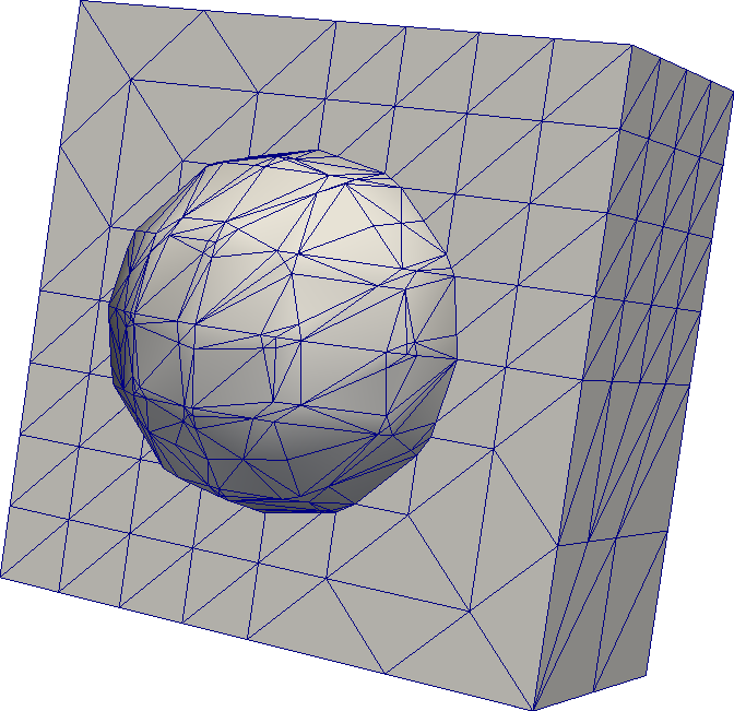
(a) $h=4.17\times 10^{-1}$

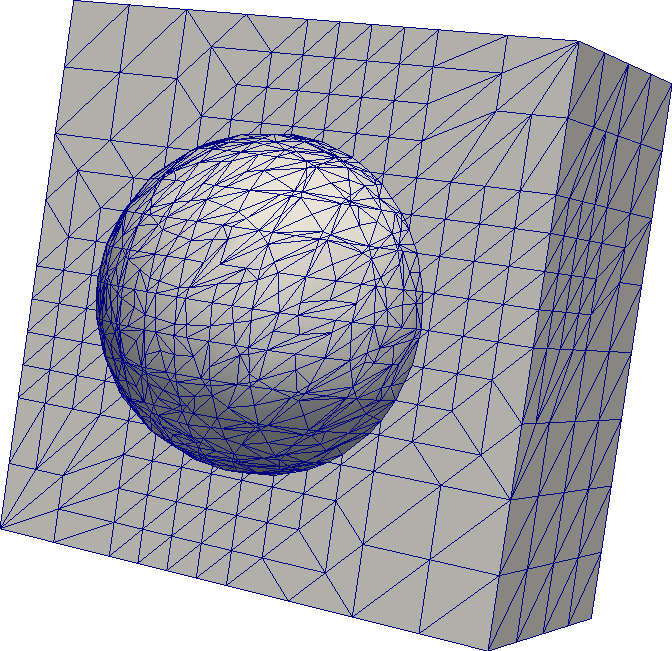
(b) $h=2.08\times 10^{-1}$

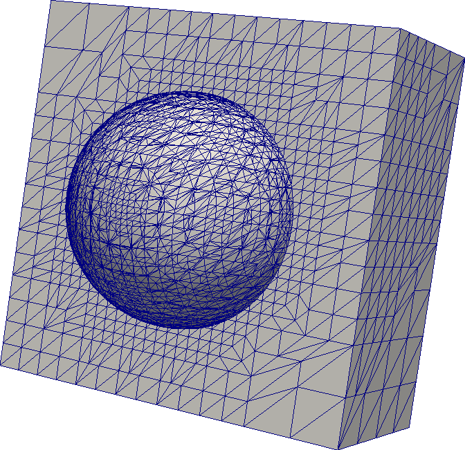
(c) $h=1.04\times 10^{-1}$

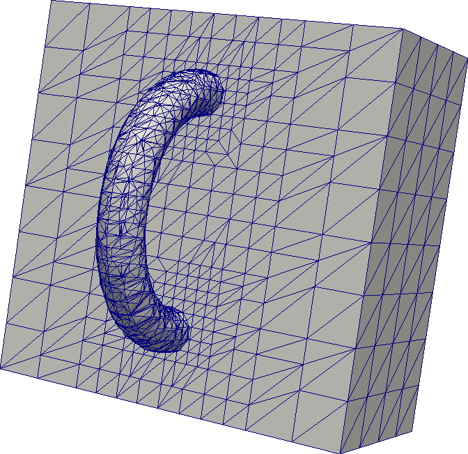
(d) $h=1.04\times 10^{-1}$

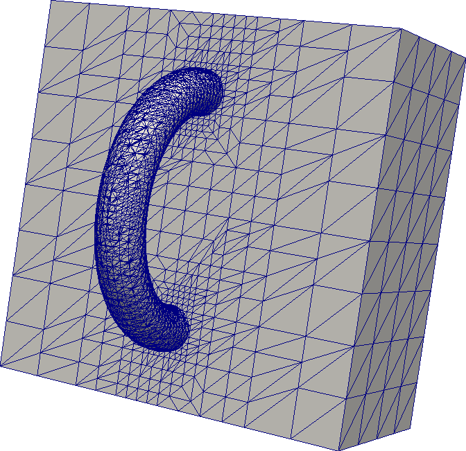
(e) $h=5.21\times 10^{-2}$

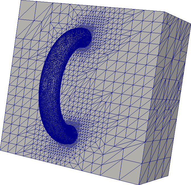
(f) $h=2.6\times 10^{-2}$

Fig. 3: Cross section of the bulk mesh and $\Gamma_{h}$ for ${\Gamma_{\text{sph}}}$ (top) and ${\Gamma_{\text{tor}}}$ (bottom), $\ell\in\{\,2,3,4\,\}$ and $\ell\in\{\,4,5,6\,\}$, respectively

In the following sections we numerically compute optimal inf-sup stability constants for $\boldsymbol{\mathbf{P}}_{2}$–$P_{1}$ and $\boldsymbol{\mathbf{P}}_{1}$–$P_{1}$ trace FEM and show convergence results for $\boldsymbol{\mathbf{P}}_{2}$–$P_{1}$ trace FEM.

6.2 Discrete inf-sup stability

Let $n\coloneqq\mbox{dim}(\mathbf{U}_{h})$ and $m\coloneqq\mbox{dim}(Q_{h})$ be the number of velocity and pressure degrees of freedom (d.o.f.). The velocity stiffness matrix $\boldsymbol{\mathbf{A}}\in\mathbb{R}^{n\times n}$, the divergence matrix $\boldsymbol{\mathbf{B}}\in\mathbb{R}^{m\times n}$, and pressure stabilization matrix $\boldsymbol{\mathbf{C}}_{\star}\in\mathbb{R}^{m\times m}$ satisfy

$$\begin{split}&\bar{\boldsymbol{\mathbf{v}}}^{T}\boldsymbol{\mathbf{A}}\bar{\boldsymbol{\mathbf{u}}}=\left\{\begin{split}A_{h}(\mathbf{u}_{h},\mathbf{v}_{h})&\quad\text{for inconsistent method,}\\ \widetilde{A}_{h}(\mathbf{u}_{h},\mathbf{v}_{h})&\quad\text{for consistent method,}\end{split}\right.\quad\\[3.44444pt] &\bar{\boldsymbol{\mathbf{q}}}^{T}\boldsymbol{\mathbf{B}}\bar{\boldsymbol{\mathbf{v}}}=b_{T}(q_{h},\mathbf{v}_{h}),\\ &\bar{\boldsymbol{\mathbf{q}}}^{T}\boldsymbol{\mathbf{C}}_{\star}\bar{\boldsymbol{\mathbf{p}}}=s(q_{h},p_{h})\end{split}$$

for all $\mathbf{u}_{h},\mathbf{v}_{h}\in\mathbf{U}_{h}$ and all $p_{h},q_{h}\in Q_{h}$. Here $\bar{\boldsymbol{\mathbf{u}}},\bar{\boldsymbol{\mathbf{v}}}\in\mathbb{R}^{n}$ and $\bar{\boldsymbol{\mathbf{p}}},\bar{\boldsymbol{\mathbf{q}}}\in\mathbb{R}^{m}$ are the velocity and pressure vectors of coefficients for the corresponding finite element functions in a standard nodal basis. The trace finite element method (21) results in the linear system

$$\begin{bmatrix}\boldsymbol{\mathbf{A}}&\phantom{-}\boldsymbol{\mathbf{B}}^{T}\\ \boldsymbol{\mathbf{B}}&-\boldsymbol{\mathbf{C}}_{\star}\\ \end{bmatrix}\begin{bmatrix}\bar{\boldsymbol{\mathbf{u}}}\\ \bar{\boldsymbol{\mathbf{p}}}\end{bmatrix}=\begin{bmatrix}\phantom{-}\bar{\boldsymbol{\mathbf{f}}}\\ -\bar{\boldsymbol{\mathbf{g}}}\end{bmatrix},$$ (73)

where $\bar{\boldsymbol{\mathbf{f}}}\in\mathbb{R}^{n}$ and $\bar{\boldsymbol{\mathbf{g}}}\in\mathbb{R}^{m}$ are load vectors for the momentum and continuity equations right-hand sides, respectively. The pressure Schur complement matrix of (73) is given by

$$\boldsymbol{\mathbf{S}}_{\star}=\boldsymbol{\mathbf{B}}\,\boldsymbol{\mathbf{A}}^{-1}\,\boldsymbol{\mathbf{B}}^{T}+\boldsymbol{\mathbf{C}}_{\star}.$$ (74)

We consider three different matrices $\boldsymbol{\mathbf{C}}_{\star}$ corresponding to three different choices of the stabilization form $s_{h}$:

1. Volume normal stabilization given in (20). We write $\boldsymbol{\mathbf{C}}_{\star}=\boldsymbol{\mathbf{C}}_{n}$ in this case;

2. The full gradient stabilization given by the bilinear form in (28) (Brezzi–Pitkäranta type stabilization). We write $\boldsymbol{\mathbf{C}}_{\star}=\boldsymbol{\mathbf{C}}_{\text{full}}$;

3. No stabilization, i.e. $\boldsymbol{\mathbf{C}}_{\star}=\boldsymbol{\mathbf{C}}_{0}\coloneqq\boldsymbol{\mathbf{0}}$.

We recall that the method analyzed in this paper corresponds to $\boldsymbol{\mathbf{C}}_{\star}=\boldsymbol{\mathbf{C}}_{n}$.

The surface pressure mass matrix $\boldsymbol{\mathbf{M}}_{0}\in\mathbb{R}^{m\times m}$ is defined through $\bar{\boldsymbol{\mathbf{q}}}^{T}\boldsymbol{\mathbf{M}}_{0}\,\bar{\boldsymbol{\mathbf{p}}}=\int_{\Gamma}p_{h}\,q_{h}\mathop{}\!\mathrm{d}{s}$. We also need auxiliary matrices

$$\boldsymbol{\mathbf{M}}_{n}\coloneqq\boldsymbol{\mathbf{M}}_{0}+\boldsymbol{\mathbf{C}}_{n},\quad\boldsymbol{\mathbf{M}}_{\text{full}}\coloneqq\boldsymbol{\mathbf{M}}_{0}+\boldsymbol{\mathbf{C}}_{\text{full}},$$ (75)

which correspond to the natural norms used in the pressure space, e.g., $\boldsymbol{\mathbf{M}}_{n}$ corresponds to $\|\cdot\|_{h}$ from (25).

We are interested in the generalized eigenvalue problem

$$\boldsymbol{\mathbf{S}}_{\star}\,\bar{\boldsymbol{\mathbf{y}}}=\lambda\,\boldsymbol{\mathbf{M}}_{\star}\,\bar{\boldsymbol{\mathbf{y}}},$$ (76)

where “$\star$” stands for “$0$,” “$n$,” or “full.” We use notation  $0=\lambda_{1}<\lambda_{2}\leq\dots\leq\lambda_{m}=O(1)$ for the generalized eigenvalues of (76). Straightforward calculations show (cf., e.g., [33, Lemma 5.9]) that for $\boldsymbol{\mathbf{S}}_{\star}=\boldsymbol{\mathbf{S}}_{n}$, $\boldsymbol{\mathbf{M}}_{\star}=\boldsymbol{\mathbf{M}}_{n}$ the smallest non-zero eigenvalue equals $c_{0}^{2}$,

$$\lambda_{2}=c_{0}^{2},$$

where $c_{0}^{2}$ is the optimal constant from the inf-sup stability condition (27) (with each term squared).

Assembling the Schur complement matrix $\boldsymbol{\mathbf{S}}_{\star}$ becomes prohibitively expensive even for rather small mesh sizes, since one needs to calculate $\boldsymbol{\mathbf{A}}^{-1}$. One possible solution is to write (76) in the mixed form:

$$\begin{split}&\begin{bmatrix}\boldsymbol{\mathbf{A}}&\phantom{-}\boldsymbol{\mathbf{B}}^{T}\\ \boldsymbol{\mathbf{B}}&-\boldsymbol{\mathbf{C}}_{\star}\\ \end{bmatrix}\begin{bmatrix}\bar{\boldsymbol{\mathbf{x}}}\\ \bar{\boldsymbol{\mathbf{y}}}\end{bmatrix}=-\lambda\>\,\begin{bmatrix}\,\,\,\boldsymbol{\mathbf{0}}\>\,\,&\\ &\boldsymbol{\mathbf{M}}_{\star}\end{bmatrix}\begin{bmatrix}\bar{\boldsymbol{\mathbf{x}}}\\ \bar{\boldsymbol{\mathbf{y}}}\end{bmatrix},\\ \text{leading to}\quad&\underbrace{\begin{bmatrix}\boldsymbol{\mathbf{A}}&\phantom{-}\boldsymbol{\mathbf{B}}^{T}\\ \boldsymbol{\mathbf{B}}&-\boldsymbol{\mathbf{C}}_{\star}\\ \end{bmatrix}}_{\mathcal{A}_{\star}}\begin{bmatrix}\bar{\boldsymbol{\mathbf{x}}}\\ \bar{\boldsymbol{\mathbf{y}}}\end{bmatrix}=-\lambda_{\epsilon}\underbrace{\begin{bmatrix}\epsilon\,\boldsymbol{\mathbf{A}}&\\ &\boldsymbol{\mathbf{M}}_{\star}\end{bmatrix}}_{\mathcal{M}^{\epsilon}_{\star}}\begin{bmatrix}\bar{\boldsymbol{\mathbf{x}}}\\ \bar{\boldsymbol{\mathbf{y}}}\end{bmatrix},\end{split}$$ (77)

with $0<\epsilon\ll 1$. Here we introduced an $\epsilon$ perturbation to the right-hand matrix to make it Hermitian positive definite. In this form, the problem is suitable for any standard generalized eigenvalue solver that operates with sparse Hermitian matrices. The spectrum of the perturbed problem consists of two sets of eigenvalues, $\mbox{sp}([\mathcal{M}^{\epsilon}_{\star}]^{-1}\mathcal{A}_{\star})=\Lambda_{\epsilon}\cup\Lambda_{\epsilon^{-1}}$. The eigenvalues from the first set converge to those of (76):

$$\lambda_{\epsilon}=\lambda+o(1)\text{ as }\epsilon\rightarrow 0,\quad\text{with }\lambda_{\epsilon}\in\Lambda_{\epsilon}\text{ and }\lambda\in\mbox{sp}(\boldsymbol{\mathbf{M}}_{\star}^{-1}\boldsymbol{\mathbf{S}}_{\star}).$$

For the eigenvalues in the other set we have $-\lambda_{\epsilon}=O(\epsilon^{-1})$, $\lambda_{\epsilon}\in\Lambda_{\epsilon^{-1}}$. This makes it straightforward for $\epsilon\ll 1$ to identify the eigenvalues we are interested in. To simplify the computation further, we replace the $(1,1)$-block of $\mathcal{M}^{\epsilon}_{\star}$ by $\epsilon\,\boldsymbol{\mathbf{I}}$.

To check that our computations are stable with respect to small $\epsilon$ and yield consistent results, we solve (77) for $\epsilon=10^{-5}$ and $\epsilon=10^{-6}$. It turns out that we obtain very close results. Furthermore, for the coarse mesh levels, when solving (76) is feasible, we also check that the dense solver for (76) and the iterative one for (77) with $\epsilon=10^{-6}$ give eigenvalues that coincide at least up to the first five significant digits.

Tables 6.2 and 6.2 report $\lambda_{2}$ (i.e. the inf-sup stability constant) and $\lambda_{m}$ (i.e. the maximum eigenvalue so that $\lambda_{m}/\lambda_{2}$ defines the effective condition number) for the following methods: 1) consistent $\boldsymbol{\mathbf{P}}_{2}$–$P_{1}$ trace finite element method (studied in this paper); 2) $\boldsymbol{\mathbf{P}}_{1}$–$P_{1}$ trace finite element method from [30]. For both discretizations we solve the eigenvalue problem (77) with different matrices $\boldsymbol{\mathbf{C}}_{\star}$ which correspond to three choices of pressure stabilization (see above).

Table 1: Extreme eigenvalues of (76) for consistent $\boldsymbol{\mathbf{P}}_{2}$–$P_{1}$ trace finite element method, $\tau=h^{-2}$, $\rho_{u}=h^{-1}$, $\rho_{p}=h$

$\Gamma={\Gamma_{\text{sph}}}$
$h$	$n$	$m$	$\boldsymbol{\mathbf{S}}_{0}$		$\boldsymbol{\mathbf{S}}_{n}$		$\boldsymbol{\mathbf{S}}_{\text{full}}$
			$\lambda_{2}$	$\lambda_{m}$	$\lambda_{2}$	$\lambda_{m}$	$\lambda_{2}$	$\lambda_{m}$
$8.33\times 10^{-1}$	$789$	$51$	$2.33\times 10^{-1}$	$1.07$	$6.3\times 10^{-1}$	$1.$	$8.81\times 10^{-1}$	$1.$
$4.17\times 10^{-1}$	$3276$	$190$	$4.72\times 10^{-2}$	$6.97\times 10^{-1}$	$5.29\times 10^{-1}$	$1.$	$7.64\times 10^{-1}$	$1.$
$2.08\times 10^{-1}$	$11718$	$664$	$7.93\times 10^{-2}$	$6.7\times 10^{-1}$	$5.09\times 10^{-1}$	$1.$	$6.39\times 10^{-1}$	$1.$
$1.04\times 10^{-1}$	$48762$	$2764$	$3.71\times 10^{-2}$	$6.69\times 10^{-1}$	$5.03\times 10^{-1}$	$1.$	$5.73\times 10^{-1}$	$1.$
$5.21\times 10^{-2}$	$193086$	$10912$	$1.81\times 10^{-3}$	$6.68\times 10^{-1}$	$4.98\times 10^{-1}$	$1.$	$5.36\times 10^{-1}$	$1.$
$2.6\times 10^{-2}$	$775998$	$43864$	$6.65\times 10^{-4}$	$6.65\times 10^{-1}$	$4.92\times 10^{-1}$	$1.$	$5.17\times 10^{-1}$	$1.$

Table 2: Extreme eigenvalues of (76) for $\boldsymbol{\mathbf{P}}_{1}$–$P_{1}$ trace finite element method, $\tau=h^{-2}$, $\rho_{u}=h$, $\rho_{p}=h$

For experiments with $\boldsymbol{\mathbf{P}}_{2}$–$P_{1}$ elements we choose parameters satisfying (22). In particular, we set $\rho_{u}=h^{-1}$ which is the upper extreme for admissible parameters, since for smaller $\rho_{u}$, the stability constant $c_{0}$ from (27) can only increase. We otherwise set $\rho_{u}=h$ for $\boldsymbol{\mathbf{P}}_{1}$–$P_{1}$ elements (which was the choice in [30]); if the resulting method is inf-sup unstable for $\rho_{u}\simeq h$, it has the same property also for larger $\rho_{u}$. In practice, to avoid extra dissipation, one would like to choose $\rho_{u}$ small but sufficient to control the condition number of $\mathbf{A}$ ($\rho_{u}\simeq h$ suits this purpose). We covered the larger range of $\rho_{u}$ by our analysis, since this may be needed if the $\boldsymbol{\mathbf{P}}_{2}$–$P_{1}$ trace FEM is extended to fluid problems on deformable surfaces.

From Table 6.2, which shows results for $\boldsymbol{\mathbf{P}}_{2}$–$P_{1}$ trace elements, we see that for $\boldsymbol{\mathbf{C}}_{0}$ (no pressure stabilization) $\lambda_{2}$ tends to zero with mesh refinement, which indicates that the discretization is not inf-sup stable. The normal gradient stabilization matrix $\boldsymbol{\mathbf{C}}_{n}$ is sufficient for the inf-sup stability, $\lambda_{2}$ is uniformly bounded from below, which confirms the main result of this paper. Of course, including the full pressure gradient term also leads to a stable method, but in this case, the method has consistency errors that are suboptimal.

For the two cases $\Gamma={\Gamma_{\text{sph}}}$ and $\Gamma={\Gamma_{\text{tor}}}$ the behavior is essentially the same. From Table 6.2 we see that only full gradient stabilization matrix $\boldsymbol{\mathbf{C}}_{\text{full}}$ guarantees inf-sup stability of $\boldsymbol{\mathbf{P}}_{1}$–$P_{1}$ trace elements, which is different to the situation with $\boldsymbol{\mathbf{P}}_{2}$–$P_{1}$ trace elements.

Next, we illustrate our claim that the optimal inf-sup stability constant $c_{0}$ in (27) is uniformly bounded with respect to the position of $\Gamma$ in the background mesh. To this end, we introduce a set of translated surfaces

$$\Gamma\mapsto\Gamma+\alpha\,\boldsymbol{\mathbf{s}},$$ (78)

with some $\alpha\in\mathbb{R}$ and $\boldsymbol{\mathbf{s}}\in\mathbb{R}^{3}$, $\|\boldsymbol{\mathbf{s}}\|=1$; see Figure 4.

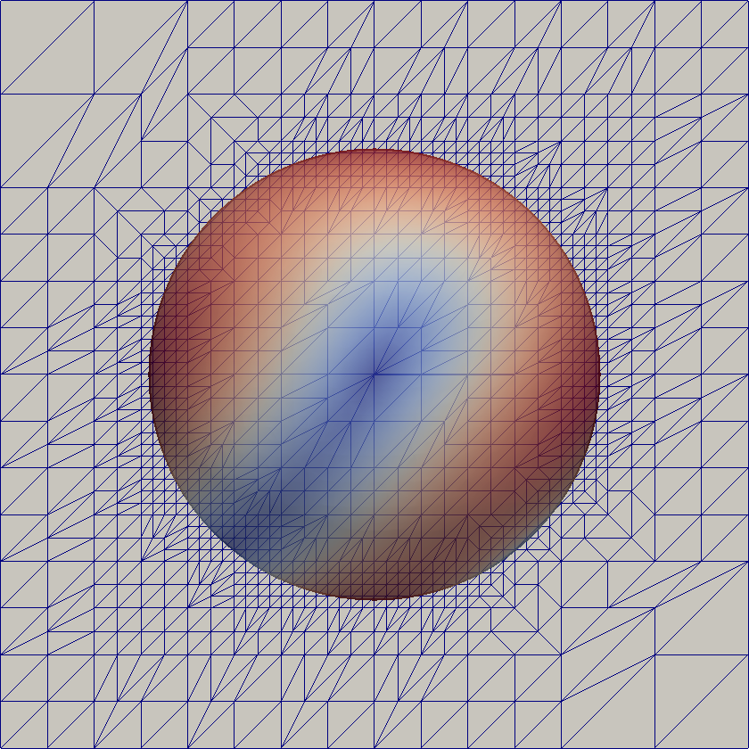
(g) ${\Gamma_{\text{sph}}}$

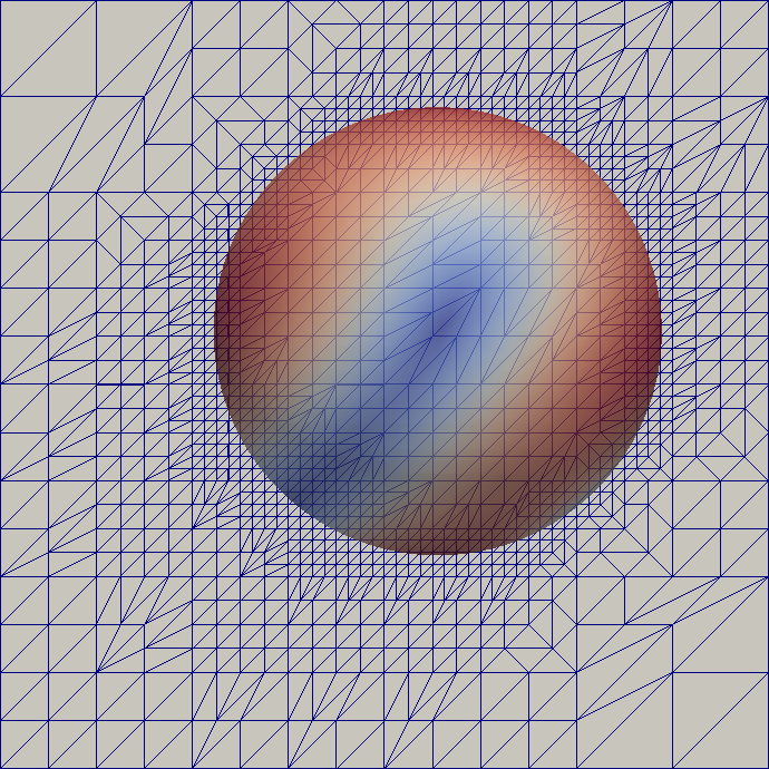
(h) ${\Gamma_{\text{sph}}}+\alpha\,\boldsymbol{\mathbf{s}}$

Fig. 4: Unit sphere (left) and the shifted unit sphere (right). Here $\boldsymbol{\mathbf{s}}=(1,1,1)^{T}/\sqrt{3}$, $\alpha=0.4$, and $h=5.21\times 10^{-2}$

We repeat eigenvalue computations for the consistent $\boldsymbol{\mathbf{P}}_{2}$–$P_{1}$ trace finite element method, with a fixed mesh size $h=1.04\times 10^{-1}$ and a varying translation parameter $\alpha$ in (78). Results are reported in Table 6.2.

Table 3: Extreme eigenvalues of (76) for perturbed surface $\Gamma+\alpha\,\boldsymbol{\mathbf{s}}$ for consistent $\boldsymbol{\mathbf{P}}_{2}$–$P_{1}$ trace finite element method, $\tau=h^{-2}$, $\rho_{u}=h^{-1}$, $\rho_{p}=h$. Here $\boldsymbol{\mathbf{s}}=(1,1,1)^{T}/\sqrt{3}$, $h=1.04\times 10^{-1}$

The results in Table 6.2 confirm the robustness of the inf-sup stability constant with respect to the position of $\Gamma$ for the method with normal gradient stabilization.

6.3 Convergence results

We set $\Gamma={\Gamma_{\text{sph}}}$ and define

$$\tilde{\boldsymbol{\mathbf{u}}}(x,y,z)\coloneqq(-z^{2},y,x)^{T},\quad\tilde{p}(x,y,z)\coloneqq x\,y^{2}+z,\quad\boldsymbol{\mathbf{u}}\coloneqq\boldsymbol{\mathbf{P}}\,\tilde{\boldsymbol{\mathbf{u}}}^{e},\quad p\coloneqq\tilde{p}^{e}.$$ (79)

Thus we have $\int_{\Gamma}p\mathop{}\!\mathrm{d}{\boldsymbol{\mathbf{x}}}=0$, $p\equiv p^{e}$, $\boldsymbol{\mathbf{u}}\equiv\boldsymbol{\mathbf{u}}^{e}$ in $\mathcal{O}(\Gamma)$, and $\boldsymbol{\mathbf{u}}$ is a tangential vector field.

Note that for our choice of ${\phi_{\text{sph}}}$ in (72) we have $\boldsymbol{\mathbf{n}}=\nabla{\phi_{\text{sph}}}/\|\nabla{\phi_{\text{sph}}}\|\equiv\boldsymbol{\mathbf{n}}^{e}$ in $\mathcal{O}(\Gamma)$. We use $P_{2}$ nodal interpolant $I^{2}_{h}(\cdot)$ defined in $\mathcal{T}_{h}^{\Gamma}$ to approximate the level-set function in our implementation. Note that for the case of the sphere ${\phi_{\text{sph}}}\in P_{2}(\mathbb{R}^{3})$ implies $I^{2}_{h}({\phi_{\text{sph}}})={\phi_{\text{sph}}}$, and so the normal vector and related operators $\boldsymbol{\mathbf{P}}$, $E_{s}$, $\boldsymbol{\mathbf{H}}$, and $\nabla_{\Gamma}$ are computed exactly.

To approximate the domain of integration, we use a sufficiently refined piecewise planar approximation of $\Gamma$,

$$\Gamma_{h}\coloneqq\{\boldsymbol{\mathbf{x}}\in\mathbb{R}^{3}\>:\>\big{(}I^{1}_{h}(\phi)\big{)}(\boldsymbol{\mathbf{x}})=0\}.$$ (80)

For the integration, we use $\Gamma_{h/m}$ with $m\simeq h^{-1}$ so that we have an $O(h^{4})$-accurate approximation of $\Gamma$.

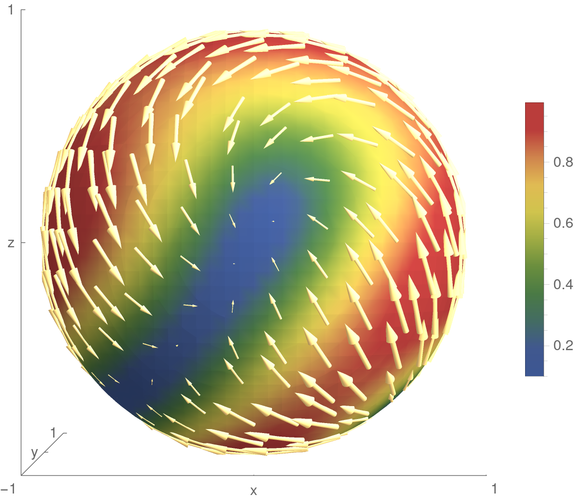
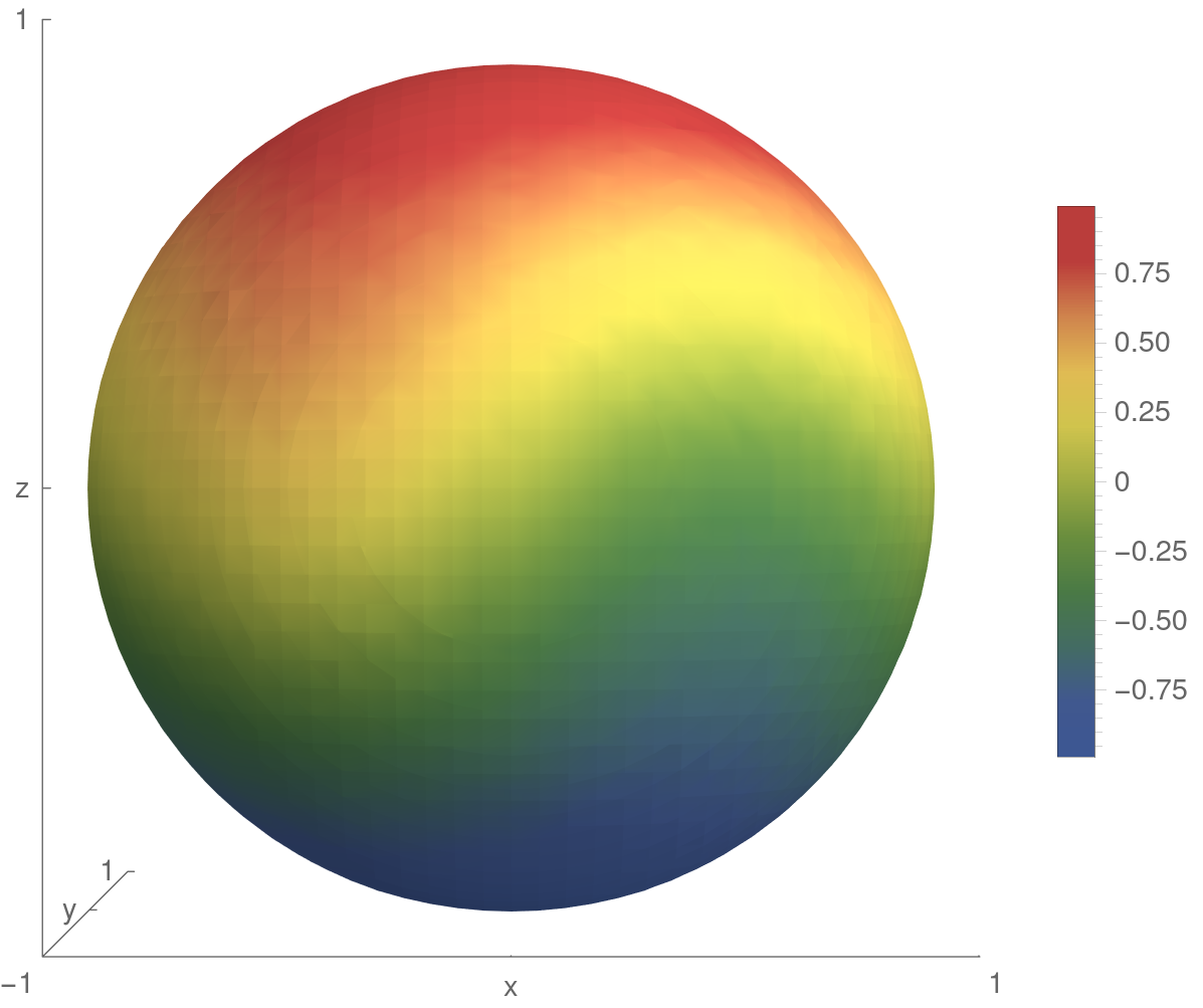
Fig. 5: Exact velocity solution (left) and pressure solution (right) as in (79)

The resulting linear system (73) is solved with MINRES as an outer solver and the block-diagonal preconditioner as defined in [30, p. 19].

Table 4: Convergence results for consistent $\boldsymbol{\mathbf{P}}_{2}$–$P_{1}$ formulation, $\tau=h^{-2}$, $\rho_{u}=h^{-1}$, $\rho_{p}=h$, and $\boldsymbol{\mathbf{C}}_{\star}=\boldsymbol{\mathbf{C}}_{n}$

Table 5: Convergence results for consistent $\boldsymbol{\mathbf{P}}_{2}$–$P_{1}$ formulation, $\tau=h^{-2}$, $\rho_{u}=h^{-1}$, $\rho_{p}=h$, and $\boldsymbol{\mathbf{C}}_{\star}=\boldsymbol{\mathbf{C}}_{\text{full}}$

We first consider the convergence rates of the (consistent) $\boldsymbol{\mathbf{P}}_{2}$–$P_{1}$ trace finite element given by (21)–(23). This corresponds to the volume normal derivative stabilization matrix $\boldsymbol{\mathbf{C}}_{n}$. Results are reported in Table 6.3. From the table we see that the consistent formulation gives optimal convergence rates in all the norms as predicted by the error analysis in section 5.

Table 6.3 reports results of a further experiment in which the volume normal derivative stabilization for the pressure is replaced by the full gradient stabilization, i.e the stabilization matrix $\boldsymbol{\mathbf{C}}_{\rm full}$ is used. This option was discussed in Remark 4.2. It is expected that this results in suboptimal convergence rates due to only $O(h^{2})$ consistency of the added term. This is what we see in Table 6.3, which shows suboptimal rates in ${L^{2}\left({\Gamma}\right)}$-velocity error norm. In both cases reported in Tables 6.3 and 6.3, the number of MINRES iterations is reasonable and stays uniformly bounded with respect to the variation of mesh parameter $h$.

7 Conclusions and outlook

The paper presented the first stability analysis of a mixed pair of $\boldsymbol{\mathbf{P}}_{2}$–$P_{1}$ finite elements for the discretization of a surface Stokes problem. For the finite element discretization of (Navier–)Stokes equations in Euclidean domains the lowest order stable Taylor–Hood element is one of the most popular methods. The results of this paper prove stability and optimal order convergence for the trace variant of the $\boldsymbol{\mathbf{P}}_{2}$–$P_{1}$ Taylor–Hood element, i.e., this method is a good candidate for discretization of fluid problems on manifolds.

Numerical experiments (not shown here) indicate that the higher order trace Taylor–Hood pairs, combined with the volume normal derivative stabilization, are also stable. In a companion paper [23] numerical results for higher order trace Taylor–Hood and a detailed comparison of the consistent and inconsistent variants are presented. That paper also addresses the issue of geometry approximation (using the parametric version of trace FEM) and the accuracy of the normal used in the penalty term. The latter issue was earlier analyzed in [20, 24] for the vector Laplace surface problem. A rigorous error analysis including geometry errors, using the isoparametric trace FEM, will be studied by the authors in a forthcoming paper.

Acknowledgement

M.O. and A.Z. were partially supported by NSF through the Division of Mathematical Sciences grant 1717516.

References

- [1] V. I. Arnold and B. A. Khesin, Topological methods in hydrodynamics, vol. 125, Springer Science & Business Media, 1999.
- [2] M. Arroyo and A. DeSimone, Relaxation dynamics of fluid membranes, Physical Review E, 79 (2009), p. 031915.
- [3] J. W. Barrett, H. Garcke, and R. Nürnberg, A stable numerical method for the dynamics of fluidic membranes, Numerische Mathematik, 134 (2016), pp. 783–822.
- [4] A. Bonito, A. Demlow, and M. Licht, A divergence-conforming finite element method for the surface stokes equation, arXiv preprint arXiv:1908.11460, (2019).
- [5] F. Brezzi and M. Fortin, Mixed and hybrid finite element methods, vol. 15, Springer Science & Business Media, 2012.
- [6] F. Brezzi and J. Pitkäranta, On the stabilization of finite element approximations of the Stokes equations, in Efficient solutions of elliptic systems, Springer, 1984, pp. 11–19.
- [7] E. Burman, S. Claus, P. Hansbo, M. G. Larson, and A. Massing, Cutfem: Discretizing geometry and partial differential equations, International Journal for Numerical Methods in Engineering, 104 (2015), pp. 472–501.
- [8] E. Burman, P. Hansbo, and M. G. Larson, A stabilized cut finite element method for partial differential equations on surfaces: The Laplace–Beltrami operator, Computer Methods in Applied Mechanics and Engineering, 285 (2015), pp. 188–207.
- [9] E. Burman, P. Hansbo, M. G. Larson, and A. Massing, Cut finite element methods for partial differential equations on embedded manifolds of arbitrary codimensions, ESAIM: Mathematical Modelling and Numerical Analysis, 52 (2018), pp. 2247–2282.
- [10] A. Demlow and M. Olshanskii, An adaptive surface finite element method based on volume meshes, SIAM Journal on Numerical Analysis, 50 (2012), pp. 1624–1647.
- [11] D. G. Ebin and J. Marsden, Groups of diffeomorphisms and the motion of an incompressible fluid, Annals of Mathematics, 92 (1970), pp. 102–163.
- [12] A. Ern and J.-L. Guermond, Theory and practice of finite elements, vol. 159, Springer Science & Business Media, 2013.
- [13] T.-P. Fries, Higher-order surface FEM for incompressible Navier–Stokes flows on manifolds, International journal for numerical methods in fluids, 88 (2018), pp. 55–78.
- [14] J. Grande, C. Lehrenfeld, and A. Reusken, Analysis of a high-order trace finite element method for PDEs on level set surfaces, SIAM Journal on Numerical Analysis, 56 (2018), pp. 228–255.
- [15] J. Grande and A. Reusken, A higher order finite element method for partial differential equations on surfaces, SIAM Journal on Numerical Analysis, 54 (2016), pp. 388–414.
- [16] M. E. Gurtin and A. I. Murdoch, A continuum theory of elastic material surfaces, Archive for Rational Mechanics and Analysis, 57 (1975), pp. 291–323.
- [17] J. Guzmán and M. Olshanskii, Inf-sup stability of geometrically unfitted Stokes finite elements, Mathematics of Computation, 87 (2018), pp. 2091–2112.
- [18] A. Hansbo and P. Hansbo, An unfitted finite element method, based on Nitsche’s method, for elliptic interface problems, Computer Methods in Applied Mechanics and Engineering, 191 (2002), pp. 5537–5552.
- [19] P. Hansbo, M. Larson, and A. Massing, A stabilized cut finite element method for the Darcy problem on surfaces, Computer Methods in Applied Mechanics and Engineering, 326 (2017), pp. 298 – 318.
- [20] P. Hansbo, M. G. Larson, and K. Larsson, Analysis of finite element methods for vector Laplacians on surfaces, IMA Journal of Numerical Analysis, (2019), p. drz018.
- [21] G. M. Hunter and K. Steiglitz, Operations on images using quad trees, IEEE Transactions on Pattern Analysis and Machine Intelligence, (1979), pp. 145–153.
- [22] T. Jankuhn, M. A. Olshanskii, and A. Reusken, Incompressible fluid problems on embedded surfaces: Modeling and variational formulations, Interfaces and Free Boundaries, 20 (2018), pp. 353–377.
- [23] T. Jankuhn and A. Reusken, Higher order trace finite element methods for the surface Stokes equation, IGPM preprint 491, (2019).
- [24] , Trace finite element methods for surface vector-Laplace equations, IGPM preprint 490. arXiv: 1904.12494. Accepted for publication in IMA J. Numer. Anal., (2019).
- [25] V. John, Finite element methods for incompressible flow problems, Springer, 2016.
- [26] H. Koba, C. Liu, and Y. Giga, Energetic variational approaches for incompressible fluid systems on an evolving surface, Quarterly of Applied Mathematics, 75 (2017), pp. 359–389.
- [27] M. Mitrea and M. Taylor, Navier-Stokes equations on Lipschitz domains in Riemannian manifolds, Mathematische Annalen, 321 (2001), pp. 955–987.
- [28] C. B. Morrey, Multiple Integrals in the Calculus of Variations, no. 130 in Die Grundlagen der mathematischen Wissenschaften in Einzeldarstellungen, Springer, 1966.
- [29] I. Nitschke, A. Voigt, and J. Wensch, A finite element approach to incompressible two-phase flow on manifolds, Journal of Fluid Mechanics, 708 (2012), pp. 418–438.
- [30] M. A. Olshanskii, A. Quaini, A. Reusken, and V. Yushutin, A finite element method for the surface Stokes problem, SIAM Journal on Scientific Computing, 40 (2018), pp. A2492–A2518.
- [31] M. A. Olshanskii and A. Reusken, Trace finite element methods for PDEs on surfaces, in Geometrically unfitted finite element methods and applications, e. a. S. Bordas, ed., vol. 121, Springer, 2017, pp. 211–258.
- [32] M. A. Olshanskii, A. Reusken, and J. Grande, A finite element method for elliptic equations on surfaces, SIAM J. Numer. Anal., 47 (2009), pp. 3339–3358.
- [33] M. A. Olshanskii and E. E. Tyrtshnikov, Iterative methods for linear systems: theory and applications, vol. 138, SIAM, 2014.
- [34] M. A. Olshanskii and V. Yushutin, A penalty finite element method for a fluid system posed on embedded surface, Journal of Mathematical Fluid Mechanics, 21 (2019), p. 14.
- [35] A. Reusken, Analysis of trace finite element methods for surface partial differential equations, IMA Journal of Numerical Analysis, 35 (2015), pp. 1568–1590.
- [36] , Stream function formulation of surface Stokes equations, IMA Journal of Numerical Analysis, (2018).
- [37] S. Reuther and A. Voigt, The interplay of curvature and vortices in flow on curved surfaces, Multiscale Modeling & Simulation, 13 (2015), pp. 632–643.
- [38] , Solving the incompressible surface Navier–Stokes equation by surface finite elements, Physics of Fluids, 30 (2018), p. 012107.
- [39] T. Sakai, Riemannian geometry, vol. 149, American Mathematical Soc., 1996.
- [40] M. E. Taylor, Analysis on Morrey spaces and applications to Navier-Stokes and other evolution equations, Communications in Partial Differential Equations, 17 (1992), pp. 1407–1456.
- [41] R. Temam, Infinite-dimensional dynamical systems in mechanics and physics, Springer, New York, 1988.
- [42] R. Verfürth, Error estimates for a mixed finite element approximation of the Stokes equations, RAIRO. Analyse numérique, 18 (1984), pp. 175–182.