AutoGMM: Automatic and Hierarchical Gaussian Mixture Modeling in Python

Abstract

Background: Gaussian mixture modeling is a fundamental tool in clustering, as well as discriminant analysis and semiparametric density estimation. However, estimating the optimal model for any given number of components is an NP-hard problem, and estimating the number of components is in some respects an even harder problem. Findings: In R, a popular package called mclust addresses both of these problems. However, Python has lacked such a package. We therefore introduce AutoGMM, a Python algorithm for automatic Gaussian mixture modeling, and its hierarchical version, HGMM. AutoGMM builds upon scikit-learn’s AgglomerativeClustering and GaussianMixture classes, with certain modifications to make the results more stable. Empirically, on several different applications, AutoGMM performs approximately as well as mclust, and sometimes better. Conclusions: AutoMM, a freely available Python package, enables efficient Gaussian mixture modeling by automatically selecting the initialization, number of clusters and covariance constraints.

1 Introduction

Clustering is a fundamental problem in data analysis where a set of objects is partitioned into clusters according to similarities between the objects. Objects within a cluster are similar to each other, and objects across clusters are different, according to some criteria. Clustering has its roots in the 1960s [1, 2], but is still researched heavily today [3, 4]. Clustering can be applied to many different problems such as separating potential customers into market segments [5], segmenting satellite images to measure land cover [6], or identifying when different images contain the same person [7].

A popular technique for clustering is Gaussian mixture modeling. In this approach, a Gaussian mixture is fit to the observed data via maximum likelihood estimation. The flexibility of the Gaussian mixture model, however, comes at the cost of hyperparameters that can be difficult to tune, and model assumptions that can be difficult to choose [4]. If users make assumptions about the model’s covariance matrices, they risk inappropriate model restriction. On the other hand, relaxing covariance assumptions leads to a large number of parameters to estimate. Users are also forced to choose the number of mixture components and how to initialize the estimation procedure.

This paper presents AutoGMM, a Gaussian mixture model based algorithm implemented in Python that automatically chooses the initialization, number of clusters and covariance constraints. Inspired by the mclust package in R, our algorithm iterates through different clustering options and cluster numbers and evaluates each according to the Bayesian Information Criterion [8]. The algorithm starts with agglomerative clustering, then fits a Gaussian mixture model with a dynamic regularization scheme that discourages singleton clusters. We compared the algorithm to mclust on several datasets, and they perform similarly.

2 Background

2.1 Gaussian Mixture Models

The most popular statistical model of clustered data is the Gaussian mixture model (GMM). A Gaussian mixture is simply a composition of multiple normal distributions. Each component has a “weight”, $w_{i}$: the proportion of the overall data that belongs to that component. Therefore, the combined probability distribution, $f(x)$ is of the form:

$$f(x)=\sum_{k=1}^{K}w_{k}f_{k}(x)=\sum_{k=1}^{K}\frac{w_{k}}{(2\pi)^{\frac{d}{2}}|\Sigma_{k}|^{-\frac{1}{2}}}\exp\left\{{\frac{1}{2}(x-\mu_{k})^{T}\Sigma_{k}^{-1}(x-\mu_{k})}\right\}$$ (1)

where $k$ is the number of clusters, $d$ is the dimensionality of the data.

The maximum likelihood estimate (MLE) of Gaussian mixture parameters cannot be directly computed, so the Expectation-Maximization (EM) algorithm is typically used to estimate model parameters [9]. The EM algorithm is guaranteed to monotonically increase the likelihood with each iteration [10]. A drawback of the EM algorithm, however, is that it can produce singular covariance matrices if not adequately constrained. The computational complexity of a single EM iteration with respect to the number of data points is $\mathcal{O}(n)$.

After running EM, the fitted GMM can be used to “hard cluster” data by calculating which mixture component was most likely to produce a data point. Soft clusterings of the data are also available upon running the EM algorithm, as each point is assigned a weight corresponding to all $k$ components.

To initialize the EM algorithm, typically all points are assigned a cluster, which is then fed as input into the M-step. The key question in the initialization then becomes how to initially assign points to clusters.

2.2 Initialization

2.2.1 Random

The simplest way to initialize the EM algorithm is by randomly choosing data points to serve as the initial mixture component means. This method is simple and fast, but different initializations can lead to drastically different results. In order to alleviate this issue, it is common to perform random initialization and subsequent EM several times, and choose the best result. However, there is no guarantee the random initializations will lead to satisfactory results, and running EM many times can be computationally costly.

2.2.2 K-Means

Another strategy is to use the k-means algorithm to initialize the mixture component means. K-means is perhaps the most popular clustering algorithm [4], and it seeks to minimize the squared distance within clusters. The k-means algorithm is usually fast, since the computational complexity of performing a fixed number iterations is $\mathcal{O}(n)$ [3]. K-means itself needs to be initialized, and k-means++ is a principled choice, since it bounds the k-means cost function [11]. Since there is randomness in k-means++, running this algorithm on the same dataset may result in different clusterings. K-means is one option in scikit-learn to perform EM initialization in its mixture.GaussianMixture class.

2.2.3 Agglomerative Clustering

Agglomerative clustering is a hierarchical technique that starts with every data point as its own cluster. Then, the two closest clusters are merged until the desired number of clusters is reached. In scikit-learn’s AgglomerativeClustering class, "closeness" between clusters can be quantified by L1 distance, L2 distance, or cosine similarity.

Additionally, there are several linkage criteria that can be used to determine which clusters should be merged next. Complete linkage, which merges clusters according to the maximally distant data points within a pair of clusters, tends to find compact clusters of similar size. On the other hand, single linkage, which merges clusters according to the closest pairs of data points, is more likely to result in unbalanced clusters with more variable shape. Average linkage merges according to the average distance between points of different clusters, and Ward linkage merges clusters that cause the smallest increase in within-cluster variance. All four of these linkage criteria are implemented in AgglomerativeClustering and further comparisons between them can be found in Everitt et al. [12].

The computational complexity of agglomerative clustering can be prohibitive in large datasets [13]. Naively, agglomerative clustering has computational complexity of $\mathcal{O}(n^{3})$. However, algorithmic improvements have improved this upper bound Murtagh [14]. Pedregosa et al. [15] uses minimum spanning tree and nearest neighbor chain methods to achieve $\mathcal{O}(n^{2})$ complexity. Efforts to make faster agglomerative methods involve novel data structures [16], and cluster summary statistics [17], which approximate standard agglomeration methods. The algorithm in Scrucca et al. [8] caps the number of data points on which it performs agglomeration by some number $N$. If the number of data points exceeds $N$, then it agglomerates a random subset of $N$ points, and uses those results to initialize the M step of the GMM initialization. So as $n$ increases beyond this cap, computational complexity of agglomeration remains constant with respect to $n$ per iteration.

2.3 Covariance Constraints

There are many possible constraints that can be made on the covariance matrices in Gaussian mixture modeling [18, 8]. Constraints lower the number of parameters in the model, which can reduce overfitting, but can introduce unnecessary bias. scikit-learn’s GaussianMixture class implements four covariance constraints (see Table 1).

Table 1: Covariance Constraints in scikit-learn’s GaussianMixture

Constraint name	Equivalent model in mclust	Description
Full	VVV	Covariances are unconstrained and can vary between components.
Tied	EEE	All components have the same, unconstrained, covariance.
Diag	VVI	Covariances are diagonal and can vary between components
Spherical	VII	Covariances are spherical and can vary between components

2.4 Automatic Model Selection

When clustering data, the user must decide how many clusters to use. In Gaussian mixture modeling, this cannot be done with the typical likelihood ratio test approach because mixture models do not satisfy regularity conditions [9].

One approach to selecting the number of components is to use a Dirichlet process model [19, 20]. The Dirichlet process is an extension of the Dirichlet distribution which is the conjugate prior to the multinomial distribution. The Dirichlet process models the probability that a data point comes from the same mixture component as other data points, or a new component altogether. This approach requires approximating posterior probabilities of clusterings with a Markov Chain Monte Carlo method, which is rather computationally expensive.

Another approach is to use metrics such as Bayesian information criterion (BIC) [21], or Akaike information criterion (AIC) [22]. BIC approximates the posterior probability of a model with a uniform prior, while AIC uses a prior that incorporates sample size and number of parameters [23]. From a practical perspective, BIC is more conservative because its penalty scales with $\ln(n)$ and AIC does not directly depend on $n$. AIC and BIC can also be used to evaluate constraints on covariance matrices, unlike the Dirichlet process model. Our algorithm, by default, relies on BIC, as computed by:

$$\text{BIC}=2\ln(\hat{L})-p\ln(n)$$ (2)

where $\hat{L}$ is the maximized data likelihood, $p$ is the number of parameters, and $n$ is the number of data points. We chose BIC as our default evaluation criteria so we can make more direct comparisons with mclust, and because it performed empirically better than AIC on the datasets presented here (not shown). However, model selection via AIC is also an option in our algorithm.

2.5 mclust

This work is directly inspired by mclust, a clustering package available only in R. The original mclust publication derived various agglomeration criteria from different covariance constraints [24]. The different covariance constraints are denoted by three letter codes. For example, "EII" means that the covariance eigenvalues are Equal across mixture components, the covariance eigenvalues are Identical to each other, and the orientation is given by the Identity matrix (the eigenvectors are elements of the standard basis).

In subsequent work, mclust was updated to include the fitting of GMMs, and the models were compared via BIC [25]. Later, model selection was made according to a modified version of BIC that avoids singular covariance matrices [26]. The most recent version of mclust was released in 2016 [8].

2.6 Comparing Clusterings

There are several ways to evaluate a given clustering, and they can be broadly divided into two categories. The first compares distances between points in the same cluster to distances between points in different clusters. The Silhouette Coefficient and the Davies-Bouldin Index are two examples of this type of metric. The second type of metric compares the estimated clustering to a ground truth clustering. Examples of this are Mutual Information, and Rand Index. The Rand Index is the fraction of times that two clusterings agree whether a pair of points are in the same cluster or different clusters. Adjusted Rand Index (ARI) corrects for chance and takes values in the interval $[-1,1]$. If the clusterings are identical, ARI is one, and if one of the clusterings is random, then the expected value of ARI is zero.

3 Methods

3.1 Datasets

We evaluate the performance of our algorithm as compared to mclust on three datasets. For each dataset, the algorithms search over all of their clustering options, and across all cluster numbers between 1 and 20.

3.1.1 Synthetic Gaussian Mixture

For the synthetic Gaussian mixture dataset, we sampled 100 data points from a Gaussian mixture with three equally weighted components in three dimensions. All components have an identity covariance matrix and the means are:

$$\mu_{0}=\begin{bmatrix}0\\ 0\\ 0\end{bmatrix},\;\mu_{1}=\begin{bmatrix}5\\ 0\\ 0\end{bmatrix},\;\mu_{2}=\begin{bmatrix}0\\ 5\\ 0\end{bmatrix},$$ (3)

We include this dataset to verify that the algorithms can cluster data with clear group structure.

3.1.2 Wisconsin Breast Cancer Diagnostic Dataset

The Wisconsin Breast Cancer Diagnostic Dataset contains data from 569 breast masses that were biopsied with fine needle aspiration. Each data point includes 30 quantitative cytological features, and is labeled by the clinical diagnosis of benign or malignant. The dataset is available through the UCI Machine Learning Repository [27]. We include this dataset because it was used in one of the original mclust publications [28]. As in Fraley and Raftery [28], we only include the extreme area, extreme smoothness, and mean texture features.

3.1.3 Spectral Embedding of Larval Drosophila Mushroom Body Connectome

Priebe et al. [29] analyzes a Drosophila connectome that was obtained via electron microscopy [30]. As in Priebe et al. [29], we cluster the first six dimensions of the right hemisphere’s adjacency spectral embedding. The neuron types, Kenyon cells, input neurons, output neurons, and projection neurons, are considered the true clustering.

3.2 AutoGMM

AutoGMM performs different combinations of clustering options and selects the method that results in the best selection criteria (AIC or BIC with BIC as default) (see Appendix for details).

1. For each of the available 10 available agglomerative techniques (from
   sklearn.cluster.AgglomerativeCluster) perform initial clustering on up to $N$ points (user specified, default value is $2000$). We also perform $K$ k-means clustering initialized with k-means++ (user specified, default value is 1).

2. Compute cluster sample means and covariances in each clustering. These are the $(10+K)$ initializations.

3. For each of the four available covariance constraints (from
   sklearn.mixture.GaussianMixture), initialize the M step of the EM algorithm with a result from Step 2. Run EM with no regularization.

   1. If the EM algorithm diverges or any cluster contains only a single data point, restart the EM algorithm, this time adding $10^{-6}$ to the covariance matrices’ diagonals as regularization.

   2. Increase the regularization by a factor of 10 if the EM algorithm diverges or any cluster contains only a single data point. If the regularization is increased beyond $10^{0}$, simply report that this GMM constraint has failed and proceed to Step 4.

   3. If the EM algorithm successfully converges, save the resulting GMM and proceed to Step 4.

4. Repeat Step 3 for all of the $(10+K)$ initializations from Step 2.

5. Repeat Steps 1-4 for all cluster numbers $k=2\ldots 10$.

6. For each of the $(10+K)\times 4\times 9$ GMM’s that did not fail, compute BIC/AIC for the GMM.

7. Select the optimal clustering—the one with the largest BIC/AIC—as the triple of (i) initialization algorithm, (ii) number of clusters, and (iii) GMM covariance constraint.

By default, AutoGMM iterates through all combinations of 10 agglomerative and 1 k-means methods (Step 1), 4 EM methods (Step 3), and $9$ cluster numbers (Step 5). However, users are allowed to restrict the set of options. AutoGMM limits the number of data points in the agglomerative step and limits the number of iterations of EM so the computational complexity with respect to number of data points is $\mathcal{O}(n)$.

The EM algorithm can run into singularities if clusters contain only a single element (“singleton clusters”), so the regularization scheme described above avoids such clusters. At first, EM is run with no regularization.

However if this attempt fails, then EM is run again with regularization. As in Pedregosa et al. [15], regularization involves adding a regularization factor to the diagonal of the covariance matrices to ensure that they are positive definite. This method does not modify the eigenvectors of the covariance matrix, making it rotationally invariant [31].

3.2.1 Hierarchical Gaussian Mixture Modeling

Built upon AutoGMM, a hierarchical version of this algorithm, HGMM, implements AutoGMM recursively on each cluster to identify potential subclusters. Specifically, HGMM estimates clusters from AutoGMM for the input data. For each of them, if the resulting number of clusters estimated by AutoGMM is 1, that cluster becomes a leaf cluster; otherwise, HGMM initiates a new level for this branch and passes data subsets associated with the estimated subclusters onto AutoGMM. The algorithm terminates when all clusters are leaf clusters.

This extension is useful for studying data with a natural hierarchical structure such as the Larval Drosophila Mushroom Body Connectome. For this dataset, hierarchical levels of a clustering may correspond to various scales of structural connectomes where a region of interest in a coarser-scaled connectome can be further classified into subtypes of neurons in a finer-scaled one. We will present clustering results on the Drosophila dataset and synthetic hierarchical Gaussian Mixture dataset.

3.3 Reference Clustering Algorithms

We compare AutoGM to two other clustering algorithms. The first, mclust v5.4.2, is available on CRAN [8]. We use the package’s Mclust function. The second, which we call GraSPyclust, uses the GaussianCluster function in graspologic. Since initialization is random in GraSPyclust, we perform clustering 50 times and select the result with the best BIC. Both of these algorithms limit the number EM iterations performed so their computational complexities are linear with respect to the number of data points. The three algorithms are compared in Table 2.

The data described before has underlying labels so we choose ARI to evaluate the clustering algorithms.

Table 2: Algorithm Comparisons. All three algorithms use Gaussian mixture modeling, but they differ in their initialization, and set of GMM constraints. Also, AutoGMM is the only algorithm that lets users perform model selection with AIC.

Algorithm	# Initializations per GMM	Initialization method	# GMM constraints	BIC	AIC	$\mathcal{O}(n)$ complexity
AutoGMM	$10+K$	Agglomeration with L1/L2/cosine distances and k-means with k-means++	4	✓	✓	✓
mclust	1	Agglomeration with likelihood-inspired distances	14	✓	$\times\color[rgb]{1,0,0}$	✓
GraSPyclust	50	K-means with k-means++	4	✓	$\times\color[rgb]{1,0,0}$	✓

3.4 Statistical Comparison

In order to statistically compare the clustering methods, we evaluate their performances on random subsets of the data. For each dataset, we take ten independently generated, random subsamples, containing 80% of the total data points. We compile ARI and Runtime data from each clustering method on each subsample. Since the same subsamples are used by each clustering method, we can perform a Wilcoxon signed-rank test to statistically evaluate whether the methods perform differently on the datasets.

We also cluster the complete data to analyze how each model was chosen, according to BIC. All algorithms were run on a 16-core machine with 120 GB of memory.

4 Results

4.1 AutoGMM

Table 3 shows the models that were chosen by each clustering algorithm on the complete datasets, and the corresponding BIC and ARI values. The actual clusterings are shown in Figures 1-3. In the synthetic dataset, all three methods chose a spherical covariance constraint, which was the correct underlying covariance structure. The GraSPyclust algorithm, however, failed on this dataset, partitioning the data into 10 clusters.

In the Wisconsin Breast Cancer dataset, the different algorithms chose component numbers of three or four, when there were only 2 underlying labels. All algorithms achieved similar BIC and ARI values. In the Drosophila dataset, all algorithms left the mixture model covariances completely unconstrained. Even though AutoGMM achieved the highest BIC, it had the lowest ARI.

In both the Wisconsin Breast Cancer dataset and the Drosophila dataset, AutoGMM achieved ARI values between 0.5 and 0.6, which are not particularly impressive. In the Drosophila data, most of the disagreement between the AutoGMM clustering, and the neuron type classification arises from the subdivision of the Kenyon cell type into multiple subgroups (Figure 3). The authors of Priebe et al. [29], who used mclust, also note this result.

Table 3: Models Chosen by Different Clustering Methods. There are 3 true clusters in the Synthetic dataset, 2 in the Breast Cancer dataset, and 4 in the Drosophila dataset. BIC indicates how well the estimated GMM parameters fit the data (higher is better). ARI indicates how well the clustering agrees with the true clustering (higher is better).

	Agglomeration	Covariance Constraint			Regularization
Dataset	AutoGMM	AutoGMM	mclust	GraSPyclust	AutoGMM
Synthetic	L2, Ward	Spherical	EII	Spherical	0
Breast Cancer	None	Diagonal	VVI	Diagonal	0
Drosophila	Cosine, Complete	Full	VVV	Full	0

	Number of Clusters
Dataset	AutoGMM	mclust	GraSPyclust
Synthetic	3	3	10
Breast Cancer	4	3	4
Drosophila	6	7	7

	BIC			ARI
Dataset	AutoGMM	mclust	GraSPyclust	AutoGMM	mclust	GraSPyclust
Synthetic	-1120	-1111	-1100	1	1	0.64
Breast Cancer	-8976	-8970	-8974	0.56	0.57	0.54
Drosophila	4608	4430	3299	0.5	0.57	0.55

Figure 1: Clustering results of different algorithms on the synthetic dataset. (b-c) AutoGMM and mclust correctly clustered the data. (c) GraSPyclust erroneously subdivided the true clusters. For visualization purposes, only the first two dimensions of the data are plotted.

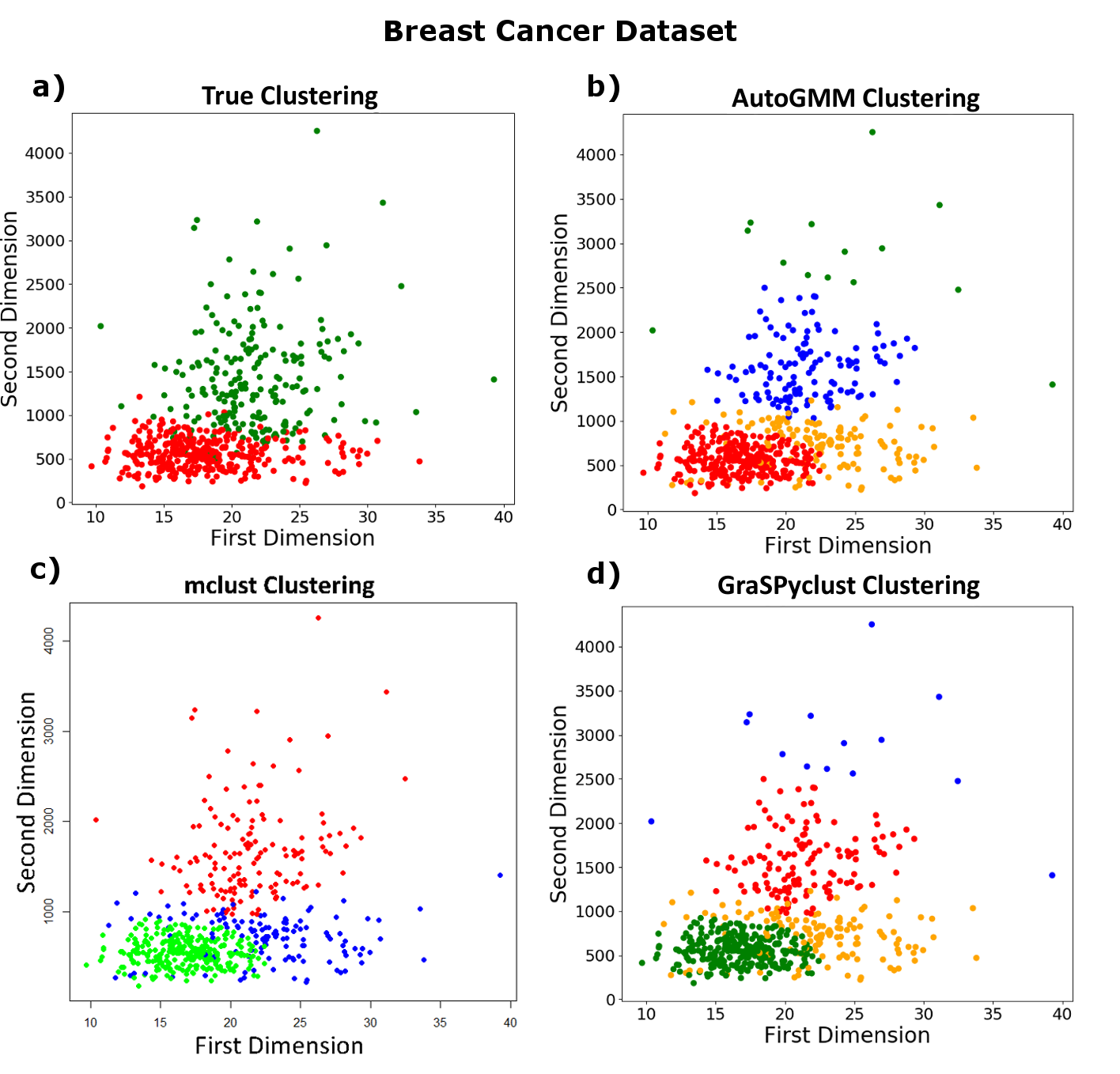
Figure 2: Clustering results of different algorithms on the breast cancer dataset. The original data was partitioned into two clusters (benign and malignant), but all algorithms here further subdivided the data into three or four clusters. For visualization purposes, only the first two dimensions of the data are plotted.

Figure 3: Clustering results of different algorithms on the drosophila dataset. There is considerable variation in the different algorithms’ results. One similarity, however, is that all algorithms subdivided the Kenyon cell cluster (red points in (a)) into several clusters. For visualization purposes, only the first two dimensions of the embedding are shown.

Figure 4 shows results from clustering random subsets of the data. The results were compared with the Wilcoxon signed-rank test at $\alpha=0.05$. On all three datasets, AutoGMM and mclust acheived similar ARI values. GraSPyclust resulted in lower ARI values on the synthetic dataset as compared to the mclust, but was not statistically different on the other datasets. Figure 4 shows that in all datasets, mclust was the fastest algorithm, and GraSPyclust was the second fastest algorithm.

Figure 5 shows the BIC curves that demonstrate model selection of AutoGMM and mclust on the Drosophila dataset. We excluded the BIC curves from GraSPyclust for simplicity. The curves peak at the chosen models.

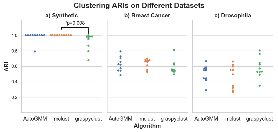
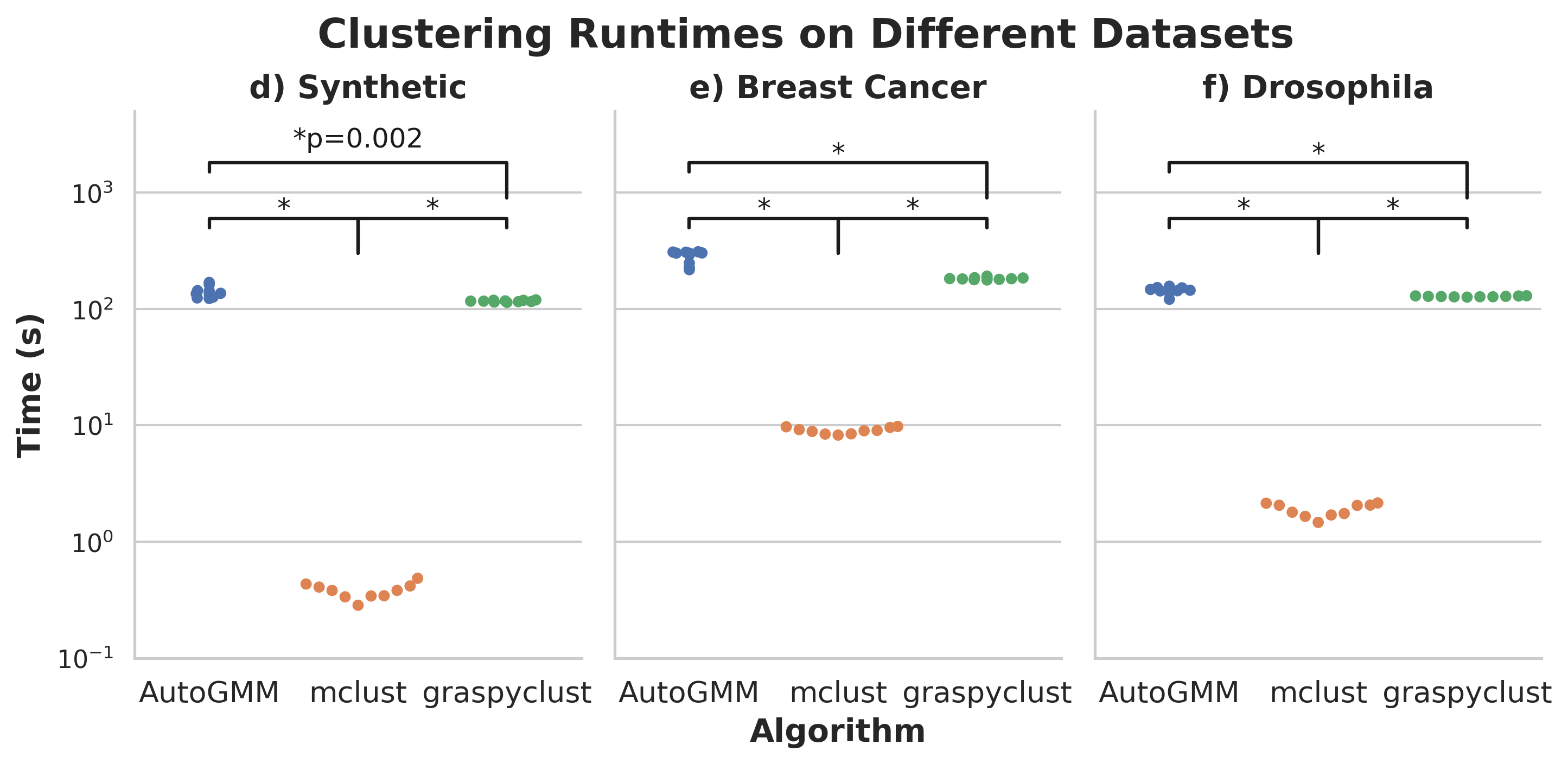
Figure 4: By clustering random subsets of the data, ARI and Runtime values can be compared via the Wilcoxon signed-rank test ($\alpha=0.05$). (a) On the synthetic dataset, GraSPyclust had a significantly lower ARI than mclust. (b), (c) There were no statistically significant differences between the algorithms on the other datasets. (d-f) mclust was the fastest algorithm, and AutoGMM the slowest, on all three datasets. The p-value was the same (0.005) for all of the statistical tests in (d-f)

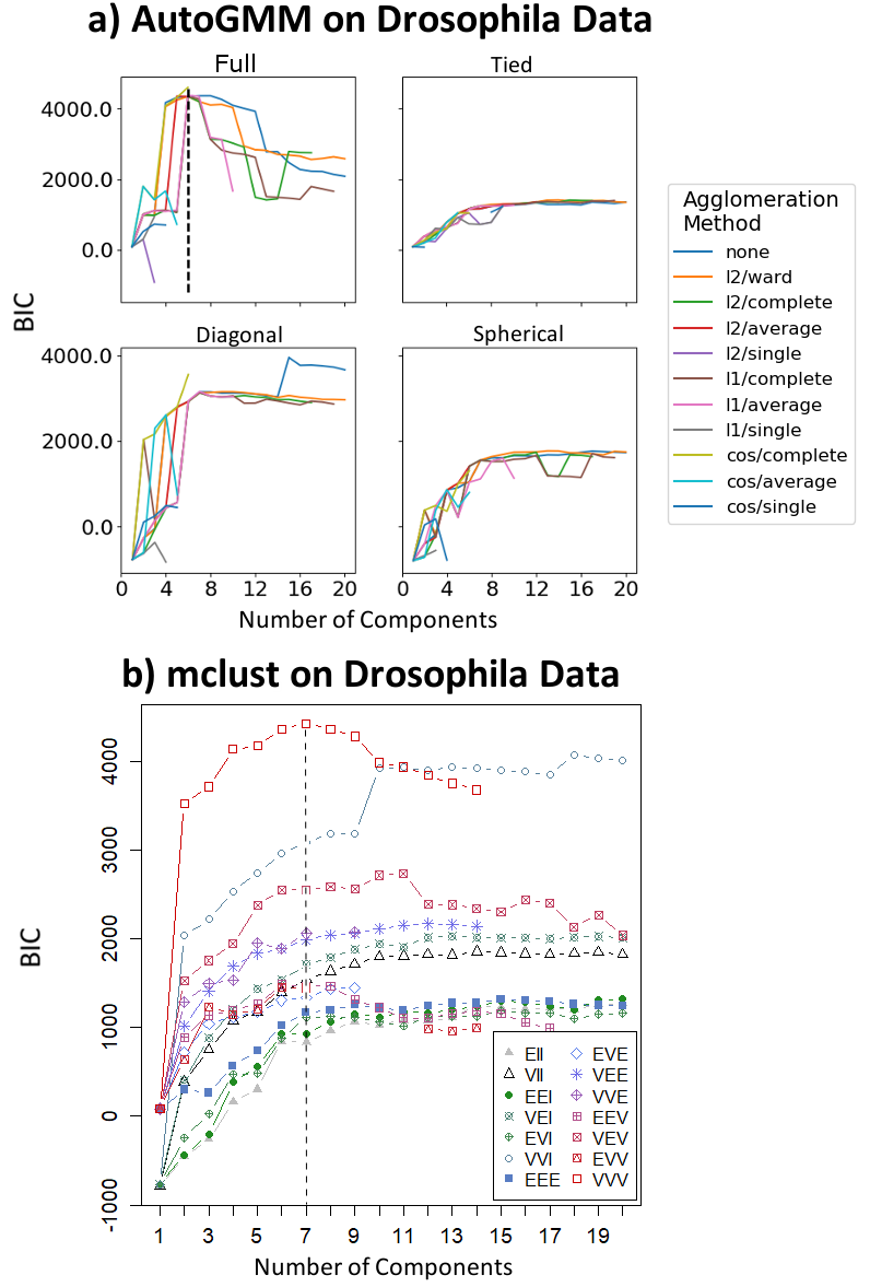
Figure 5: BIC values of all clustering options in AutoGMM and mclust on the Drosophila dataset. (a) There are 44 $(11\times 4)$ total clustering options in AutoGMM. Each curve corresponds to an agglomeration method (’none’ means performing k-means instead of agglomerative clustering), and each subplot corresponds to a covariance constraint (Table 1). (b) The 14 curves correspond to the 14 clustering options in mclust. The chosen models, from Table 3, are marked with a vertical dashed line. Missing or truncated curves indicate that the algorithm did not converge to a satisfactory solution at those points.

Figure 6: Clustering runtimes on datasets of varying size. Each algorithm has several clustering options, and each dotted line corresponds to one of these options. The solid lines are a linear regression between $\log(\#\text{ of samples})$ and $\log(\#\text{ of seconds})$ on the large datasets. The slopes of these regressions are shown in the legend, and approximate the order of the computational complexity with respect to the number of data points ($n$). All clustering methods seem to scale linearly with $n$, as expected. Each dataset contains randomly generated data from a three component Gaussian mixture in three dimensions, as described before.

We also investigated how algorithm runtimes scale with the number of data points. Figure 6 shows how the runtimes of all clustering options of the different algorithms scale with large datasets. We used linear regression on the log-log data to estimate computational complexity. The slopes for the AutoGMM, mclust, and GraSPyclust runtimes were $0.55$, $0.67$, and $0.57$ respectively. This supports our calculations that the runtime of the three algorithms is linear with respect to $n$.

In addition to mclust and GraSPyclust, AutoGMM was compared to other state of the art clustering techniques including k-means, agglomerative clustering, and two variants of a naive selection of Gaussian mixture models. For k-means and agglomerative clustering, the model with the highest ARI is considered to be the best one. The hyperparameters include the number of initializations used in k-means, the affinity and linkage criteria in agglomeration, and the number of clusters for both algorithms. Moreover, unlike our automatic model selection procedure used in AutoGMM, Gaussian mixture model selection can be performed by simply searching over all models with different parameters such as the number of components and the covariance type, and choose the one with the best BIC value [32]. Both the cases of performing one or multiple K-means initializations will be evaluated. We demonstrate their performances on a two-dimensional synthetic double-cigar dataset which is comprised of $100\times 2$ random samples drawn from two Gaussian distributions with means $\mu_{0}=[-3,0],\mu_{1}=[3,0]$ and the same covariance matrix $\begin{bmatrix}1&0\\ 0&200\end{bmatrix}$. Searching over all cluster numbers in $[2,5]$, only AutoGMM recovered the two-cluster structure of the dataset shown in Figure 7 (top). Averaged over 100 trials, AutoGMM outperforms all other algorithms in terms of ARI for this dataset (Figure 7). Interestingly, even by only increasing the number of k-means initializations for the Naive GM case, ARIs increased significantly (Wilcoxon sign-rank test p-value $<0.005$).

Figure 7: Clustering results on the double-cigar dataset for various clustering algorithms. Top: estimated labels for one realization of the data by each algorithm. An ARI score comparing the estimated labels and the true labels is located in the top right corner of each panel. For k-means clustering, the number of initializations was set to 10, and the model resulting in the estimation with the highest ARI was selected. For agglomerative clustering, all possible combinations of affinity and linkage (10 in total) were considered and the model selected has the highest ARI. For each of the three other Gaussian mixture mode based algorithms, the best model is the one with the best BIC value. In particular, the number of k-means initialization for the Naive GM was set to either 1 or 10 (multi init), and was set to 10 for AutoGMM. The number of components or clusters to consider was in $[2,5]$ for all algorithms. Bottom: ARIs for all clustering algorithms over 100 realizations.

4.2 HGMM

We evaluated the performance of HGMM on synthetic hierarchical Gaussian mixture data. We sampled $8\times 100$ data points from eight Gaussian distributions (100 from each) in one dimension with standard deviation $0.5$ and of means in the range of $[-15,15]$. The data can be grouped into a 3-level hierarchy: eight clusters of one-component Gaussian at the finest level, four clusters of 2-component Gaussian mixture at the middle level, and two clusters of 4-component Gaussian mixture at the coarsest level (Figure 8a).

HGMM was applied to the synthetic data described above; in this experiment, the maximum number of components was two at each iteration. The resulting clustering dendrogram was cut at various depths to form flat clusterings. A flat clustering cut at depth $d$ contains the cluster assignments from all leaf nodes, each of which has a maximum depth of $d$. Those flat clusterings were evaluated in terms of ARI scores. In Figure 8b, each cluster at each depth is denoted by a unique color, and each node in the dendrogram in Figure 8c is colored by its predicted cluster. The 800 data points were sorted in increasing order (since they lie on a line). HGMM perfectly classifies the data into two or four clusters at depth of one or two, respectively (Figure 8b). The 8 Gaussian mixture components are not perfectly separable (as indicated by Figure 8a), but the flat clustering cut at depth three or four still achieves a relatively high ARI computed against the classification of eight clusters (Figure 8b).

A total of 50 sets of synthetic hierarchical data were generated and clustered by HGMM in the same way as above. Each of the 50 dendrograms was cut at all possible depths resulting in a set of flat clusterings. At depth one, the clusterings of all 50 datasets were perfect (Figure 8c). Similarly, all flat clusterings cut at depth two perfectly reveal the middle-level partition of the data (Figure 8c). Most dendrograms were not terminated at depth three as in the true dendrogram (Figure 8c), while most leaf clusterings resemble closely the finest classification into eight clusters suggested by an ARI of approximately $0.9$ (Figure 8c). Moreover, the number of clusters in most leaf clusterings is approximately 10 (Figure 8d).

Figure 8: Clustering performance of HGMM on synthetic hierarchical data. (a) Distribution of hierarchical simulation data (average over 100 sets). Each set of data can be grouped at three levels into 8, 4 or 2 clusters, respectively. The colored labels correspond to the 8 cluster classification. (b) Clustering assignments of one set of hierarchical synthetic data suggests perfect or near-perfect clustering by HGMM across depths of the dendrogram. Each of the sorted data points was colored according to the assigned cluster by HGMM at each flat clustering. Rows correspond to the flat clusterings cut at the depths of 1 to the maximum depth that were evaluated against the true clusterings of $[2,4,8,8]$ clusters, respectively. Columns next to the dendrogram specify the number of clusters at each depth and the ARI score of the corresponding flat clustering, respectively. (c) Each flat clustering at the depth of 1, 2 or more was compared to the true clustering of $[2,4,8]$ clusters, respectively, to generate an ARI score. A truncated curve indicates that some of the depths to cut exceed the maximum depth of the resulting clustering. (d) The number of clusters in the leaf clustering was computed for each of 50 trials. The red dotted line indicates the true number of clusters. Most leaf clusterings have a similar number of clusters as the truth.

4.2.1 HGMM on Real Data

To further illustrate the performance of HGMM, we studied its application to the Drosophila dataset which was assumed to possess a natural hierarchical structure of neuron types. For both hemispheres of the connectome, we implemented HGMM with a maximum of six components (the estimated number of clusters by AutoGMM shown before) on the first six dimensions of the adjacency spectral embedding, and plotted the dendrogram up to depth two. Notice that the depth-one clustering of the right hemisphere by HGMM is the same as the estimation from AutoGMM reported before (Figure 3b).

Recursively clustering at depth two results in fewer clusters of mixed neuron types on both hemispheres (Figure 9). This suggests that HGMM could be useful for revealing neuron types and subtypes on finer scales, paving way towards a better understanding of how various scales of structural domains relate to activities.

Figure 9: Hierarhical clustering result of HGMM on the Drosophila dataset. At each depth, the maximum number of components was set to 6. Each bar in either dendrogram represents a cluster with a width proportional to the number of neurons in that cluster. Neurons in each bar was colored according to its true label. Unlike projection neurons (PN), input neurons (MBIN) or output neurons (MBON), Kenyon cells (KC) were colored based on three subclasses, young (KC(y)), multi-claw (KC(m)), and single-claw (KC(s)). Clusters at depth one mostly contain neurons from the same major class while most leaf clusters contain neurons from the same subclass.

5 Discussion

In this paper we present an algorithm, AutoGMM, that performs automatic model selection for Gaussian mixture modeling in Python. To the best of our knowledge, this algorithm is the first of its kind that is freely available in Python. AutoGMM iterates through 44 combinations of clustering options in Python’s scikit-learn package and chooses the GMM that achieves the best BIC. The algorithm avoids Gaussian mixtures whose likelihoods diverge, or have singleton clusters.

AutoGMM was compared to mclust, a state of the art clustering package in R, and achieved similar BIC and ARI values on three datasets. Results from the synthetic Gaussian mixture (Table 3, Figure 1) highlight the intuition behind AutoGMM’s regularization scheme. GraSPyclust did not perform well on the synthetic data, because it erroneously subdivided the 3 cluster data into 10 clusters. AutoGMM avoids this problem because its regularization does not allow singleton clusters. In all fairness, GraSPyclust’s performance on subsets of the synthetic data (Figure 4) is much better than its performance on the complete data. However, its random initialization leaves it more susceptible to inconsistent results.

Figure 4, shows that on our datasets, mclust is the fastest algorithm. However, computational complexity of all algorithms is linear with respect to the number of data points, and this is empirically validated by Figure 6. Thus, mclust is faster by only a constant factor. Several features of the mclust algorithm contribute to this factor. One is that much of the computation in mclust is written in Fortran, a compiled programming language. AutoGMM and GraSPyclust, on the other hand, are written exclusively in Python, an interpreted programming language. Compiled programming languages are typically faster than interpreted ones. Another is that mclust evaluates fewer clustering methods (14) than AutoGMM (44). Indeed, using AutoGMM trades runtime for a larger space of GMMs. However, when users have an intuition into the structure of the data, they can restrict the modeling options and make the algorithm run faster.

One opportunity to speed up the runtime of AutoGMM would involve a more principled approach to selecting the regularization factor. Currently, the algorithm iterates through 8 fixed regularization factors until it achieves a satisfactory solution. However, the algorithm could be improved to choose a regularization factor that is appropriate for the data at hand.

The most obvious theoretical shortcoming of AutoGMM is that there is no explicit handling of outliers or singleton clusters. Since the algorithm does not allow for clusters with only one member, it may perform poorly with stray points of any sort. Future work to mitigate this problem could focus on the data or the model. Data-based approaches include preprocessing for outliers, or clustering subsets of the data. Alternatively, the model could be modified to allow singleton clusters, while still regularizing to avoid singularities.

In the future, we are interested in high dimensional clustering using statistical models. The EM algorithm, a mainstay of GMM research, is even more likely to run into singularities in high dimensions, so we would need to modify AutoGMM accordingly. One possible approach would use random projections, as originally proposed by Dasgupta [33] in the case where the mixture components have means that are adequately separated, and the same covariance. Another approach would involve computing spectral decompositions of the data, which can recover the true clustering and Gaussian mixture parameters under less restrictive conditions [34, 35].

6 Availability of source code and requirements

• Project name: AutoGMM

• Project home page: https://github.com/tliu68/autogmm

• Operating system(s): Platform independent

• Programming language: Python 3

• License: MIT Licence

7 Data Availability

The data sets supporting the results of this article are available in the Machine Learning Databases [27] and MBconnectome repositories [29]. Together with the code, they are also available in the computational capsule on CodeOcean at https://codeocean.com/capsule/0363761/tree/v1.

8 Additional Files

Supplemental File 1: Algorithms of AutoGMM.

9 Competing Interests

The authors declare that they have no competing interests.

10 Funding

Research was partially supported by funding from Microsoft Research. This material is based upon work supported by the National Science Foundation Graduate Research Fellowship under Grant No. DGE1746891.

11 Author’s Contributions

T.L.A.: Conceptualization, Methodology, Data curation, Software, Formal Analysis, Visualization, Writing – original draft, Writing – review & editing. B.D.P.: Software, Writing – review & editing. T.L.: Software, Visualization, Writing – review & editing. J.T.V.: Conceptualization, Methodology, Funding acquisition, Supervision, Writing – review & editing.

12 Appendix

Note: The algorithm descriptions here use BIC as the selection criteria. Our implementation allows for the use of AIC as well.

Algorithm 1 AutoGMM works by performing an initial clustering, then fitting a GMM. The GMM with the best BIC is identified, and used to cluster the data. The 44 available clustering options are composed of [(10 agglomeration methods + k-means) for initialization] $\times$ [4 covariance constraints in EM]. By default, AutoGMM iterates through all 44 clustering options for all cluster numbers ($k$) from 2 to 20. However, users can modify the range of cluster numbers, and restrict the algorithm to a subset of the clustering options. Lastly, our algorithm saves the results of all clustering options, but those details are beyond the scope of this pseudocode.

1:

• $X\in\operatorname{R}^{n\times d}$ - $n$ samples of $d$-dimensional data points.

Optional:

• $K_{min}$ - minimum number of clusters, default to 2.

• $K_{max}$ - maximum number of clusters, default to 20.

• affinities - affinities to use in agglomeration, subset of $[L2,L1,cosine,none]$, default to all. Note: $none$ indicates the k-means initialization option, so it is not paired with linkages.

• linkages - linkages to use in agglomeration, subset of $[ward,complete,average,single]$, default to all. Note: $ward$ linkage is only compatible with $L2$ affinity.

• cov_constraints - covariance constraints to use in GMM, subset of $[full,tied,diag,spher$- $ical]$, default to all.

2:

• best_clustering - label vector in $[1...K_{max}]^{n}$ indicating cluster assignment

• best_k - number of clusters

• best_init - initialization method

• best_cov_constraint - covariance constraint

• best_reg_covar - regularization factor

Algorithm 1 continued

1:function AutoGMM($X$, $K_{min}$,$K_{max}$,affinities, linkages, cov_constraints)

2:     $ks$ = $[K_{min},...,K_{max}]$

3:     best_bic = $None$

4:     for $k$ in $ks$ do

5:         for affinity in affinities do

6:              for linkage in linkages do $\triangleright$ ward linkage is only compatible with L2 affinity

7:                  if affinity $\neq$ none then

8:                       $X\_subset$ = Subset($X$) $\triangleright$ Algorithm 2

9:                       init = sklearn.cluster.AgglomerativeCluster($k$,affinity,linkage).fit_predict($X\_subset$) $\triangleright$ Pedregosa et al., 2011

10:                  else

11:                       init = $None$ $\triangleright$ Use the default initialization of GaussianMixture $\triangleright$ which is 1 repetition of k-means++ followed by k-means

12:                  end if

13:                  for cov_constraint in cov_constraints do

14:                       clustering, bic, reg_covar = GaussianCluster ($X$, $k$, cov_constraint, init) $\triangleright$ Algorithm 3

15:                       if best_bic $=None$ or bic $>$ best_bic then

16:                           best_bic = bic

17:                           best_clustering = clustering

18:                           best_k = $k$

19:                           best_init = [affinity, linkage]

20:                           best_cov_constraint = cov_constraint

21:                           best_reg_covar = reg_covar

22:                       end if

23:                  end for

24:              end for

25:         end for

26:     end for

27:end function

Algorithm 2 Sample a random subset of the data if the number of data points ($n$) exceeds 2000. So, for $n>2000$, computational complexity of agglomeration is constant with respect to $n$.

1:$X\in\operatorname{R}^{n\times d}$ - $n$ samples of $d$-dimensional data points.

2:$X\_subset$ - random subset of the data.

3:function Subset($X$)

4:     n_samples = length($X$) $\triangleright$ Number of data points

5:     if n_samples $>2000$ then

6:         $X\_subset=$ RandomSubset($X,2000$) $\triangleright$ Sample 2000 random data points

7:     else

8:         $X\_subset=X$

9:     end if

10:end function

Algorithm 3 Regularized Gaussian Cluster. Initially, the algorithm attempts to fit a GMM without regularization. If the EM algorithm diverges, or if the GMM clustering has a cluster with a single data point (“singleton cluster"), then EM is repeated with a higher regularization. If there continue to be singleton clusters even when the regularization is increased to a certain point (1), then this clustering attempt terminates and is considered a failure.

1:

• $X\in\operatorname{R}^{n\times d}$ - $n$ samples of $d$-dimensional data points.

• $k$ - number of clusters.

• cov_constraint - covariance constraint.

Optional:

• init - initialization.

2:

• $y$ - cluster labels.

• bic - Bayesian Information Criterion.

• reg_covar - regularization factor.

3:function GaussianCluster($X$, $k$, cov_constraint, init)

4:     if init $\neq None$ then

5:         weights_init, means_init, precisions_init = EstimateGaussianParameters ($X$, init) $\triangleright$ Compute sample weight, mean and precision for each cluster

6:     else

7:         weights_init, means_init, precisions_init = $None$, $None$, $None$

8:     end if

9:     reg_covar = $0$

10:     bic = $None$

11:     converged = $False$

12:     while reg_covar $\leq 1$ and converged $=False$ do

13:         gmm = sklearn.mixture.GaussianMixture(k,cov_constraint, reg_covar,weights_init,means_init,precisions_init) $\triangleright$ Pedregosa et al., 2011

14:         $y$ = gmm.fit_predict(X) $\triangleright$ EM algorithm

15:         if SingletonCluster($y$) or EMError then      $\triangleright$ If there is a singleton cluster, or if EM failed

16:              reg_covar = IncreaseReg(reg_covar) $\triangleright$ Algorithm 4

17:         else

18:              bic = gmm.bic()

19:              converged = $True$

20:         end if

21:     end while

22:end function

Algorithm 4 Increase Covariance Regularization Factor. The lowest nonzero regularization factor is $10^{-6}$, which is subsequently increased by a factor of 10.

1:reg_covar - current covariance regularization factor.

2:reg_covar_new - incremented covariance regularization factor.

3:function IncreaseReg(reg_covar)

4:     if reg_covar $=0$ then

5:         reg_covar_new $=10^{-6}$

6:     else

7:         reg_covar_new $=$ reg_covar $\times 10$

8:     end if

9:end function

References

- MacQueen [1967] MacQueen J. Some methods for classification and analysis of multivariate observations. In: Proceedings of the Fifth Berkeley Symposium on Mathematical Statistics and Probability, Volume 1: Statistics; 1967. p. 281–297.
- Davis [1967] Davis JA. Clustering and Structural Balance in Graphs. Human Relations 1967;20:181–187.
- Saxena et al. [2017] Saxena A, Prasad M, Gupta A, Bharill N, Patel OP, Tiwari A, et al. A Review of Clustering Techniques and Developments. Neurocomputing 2017;267:664–681.
- Jain [2010] Jain AK. Data Clustering: 50 Years Beyond K-means. Pattern Recognition Letters 2010 June;31(8):651–666.
- Jurowski and Reich [2000] Jurowski C, Reich AZ. An Explanation and Illustration of Cluster Analysis for Identifying Hospitality Market Segments. Journal of Hospitality & Tourism Research 2000;24:67–91.
- Bandyopadhyay [2005] Bandyopadhyay S. Satellite image classification using genetically guided fuzzy clustering with spatial information. International Journal of Remote Sensing 2005;26(3):579–593.
- Otto et al. [2018] Otto C, Wang D, Jain AK. Clustering Millions of Faces by Identity. IEEE Transactions on Pattern Analysis and Machine Intelligence 2018;40(2).
- Scrucca et al. [2016] Scrucca L, Fop M, Murphy TB, Raftery AE. mclust 5: clustering, classification and density estimation using Gaussian finite mixture models. The R Journal 2016;8(1):205–233.
- McLachlan and Peel [2000] McLachlan G, Peel D. Finite mixture models. New York: John Wiley & Sons; 2000.
- Dempster et al. [1977] Dempster AP, Laird NM, Rubin DB. Maximum likelihood from incomplete data via the EM algorithm. Journal of the Royal Statistical Society, Series B 1977;39(1):1–38.
- Arthur and Vassilvitskii [2007] Arthur D, Vassilvitskii S. K-means++: The Advantages of Careful Seeding. In: Proceedings of the Eighteenth Annual ACM-SIAM Symposium on Discrete Algorithms; 2007. p. 1027–1035.
- Everitt et al. [2011] Everitt BS, Landau S, Leese M. Cluster Analysis. 5th ed. John Wiley & Sons; 2011.
- Xu and Wunsch [2009] Xu R, Wunsch D. Clustering, vol. 10. Hoboken, New Jersey: John Wiley & Sons; 2009.
- Murtagh [1983] Murtagh F. A survey of recent advances in hierarchical clustering algorithms. The Computer Journal 1983;26:354–359.
- Pedregosa et al. [2011] Pedregosa F, Varoquaux G, Gramfort A, Michel V, Thirion B, Grisel O, et al. Scikit-learn: Machine Learning in Python. Journal of Machine Learning Research 2011;12(12):2825–2830.
- Zhang et al. [1997] Zhang T, Ramakrishnan R, Livny M. BIRCH: A New Data Clustering Algorithm and Its Applications. Data Mining and Knowledge Discovery 1997;1:141–182.
- Guha et al. [1998] Guha S, Rastogi R, Shim K. CURE: An Efficient Clustering Algorithm for Large Databases. In: Proceedings of the ACM SIGMOD Conference; 1998. .
- Bouveyron and Brunet-Saumard [2014] Bouveyron C, Brunet-Saumard C. Model-based clustering of high-dimensional data: A review. Comput Stat Data Anal 2014;71:52–78.
- Rasmussen [1999] Rasmussen CE. The Infinite Gaussian Mixture Model. In: Proceedings of the 12th International Conference on Neural Information Processing Systems; 1999. p. 554–560.
- Ferguson [1973] Ferguson TS. A Bayesian Analysis of Some Nonparametric Problems. The Annals of Statistics 1973;1(2):209–230.
- Schwarz [1978] Schwarz G. Estimating the Dimension of a Model. The Annals of Statistics 1978;6(2):461–464.
- Akaike [1974] Akaike H. A new look at the statistical model identification. IEEE Transactions on Automatic Control 1974;19:716–723.
- Burnham and Anderson [2004] Burnham KP, Anderson DR. Multimodel Inference: Understanding AIC and BIC in Model Selection. Sociological Methods & Research 2004;33(2):261–304.
- Banfield and Raftery [1993] Banfield JD, Raftery AE. Model-Based Gaussian and Non-Gaussian Clustering. Biometrics 1993;49:803–821.
- Dasgupta and Raftery [1998] Dasgupta A, Raftery AE. Detecting Features in Spatial Point Processes with Clutter via Model-Based Clustering. Journal of the American Statistical Association 1998;93(441):294–302.
- Fraley and Raftery [2007] Fraley C, Raftery AE. Bayesian Regularization for Normal Mixture Estimation and Model-Based Clustering. Journal of Classification 2007 Sep;24(2):155–181.
- Dua and Graff [2017] Dua D, Graff C, UCI Machine Learning Repository; 2017. http://archive.ics.uci.edu/ml.
- Fraley and Raftery [2002] Fraley C, Raftery AE. Model-Based Clustering, Discriminant Analysis, and Density Estimation. Journal of the American Statistical Association 2002;97(458):611–631.
- Priebe et al. [2017] Priebe CE, Park Y, Tang M, Athreya A, Lyzinski V, Vogelstein JT, et al. Semiparametric spectral modeling of the Drosophila connectome. arXiv preprint arXiv:170503297 2017;.
- Eichler et al. [2017] Eichler K, Li F, Litwin-Kumar A, Park Y, Andrade I, Schneider-Mizell CM, et al. The complete connectome of a learning and memory center in an insect brain. Nature 2017;548.
- Ledoit and Wolf [2004] Ledoit O, Wolf M. A well-conditioned estimator for large-dimensional covariance matrices. Journal of Multivariate Analysis 2004;88:365–411.
- skl [2021] Gaussian Mixture Model Selection; 2021. https://scikit-learn.org/stable/auto_examples/mixture/plot_gmm_selection.html#gaussian-mixture-model-selection.
- Dasgupta [1999] Dasgupta S. Learning mixtures of Gaussians. In: 40th Annual Symposium on Foundations of Computer Science (Cat. No. 99CB37039) IEEE; 1999. p. 634–644.
- Vempala and Wang [2004] Vempala S, Wang G. A spectral algorithm for learning mixture models. Journal of Computer and System Sciences 2004;68(4):841–860.
- Achlioptas and McSherry [2005] Achlioptas D, McSherry F. On spectral learning of mixtures of distributions. In: International Conference on Computational Learning Theory Springer; 2005. p. 458–469.