Evolutionary models for R Coronae Borealis stars

Abstract

We use Modules for Experiments in Stellar Astrophysics (MESA) to construct stellar evolution models that reach a hydrogen-deficient, carbon-rich giant phase like the R Coronae Borealis (R CrB) stars. These models use opacities from OPAL and ÆSOPUS that cover the conditions in the cool, H-deficient, CNO-enhanced envelopes of these stars. We compare models that begin from homogeneous He stars with models constructed to reproduce the remnant structure shortly after the merger of a He and a CO white dwarf (WD). We emphasize that models originating from merger scenarios have a thermal reconfiguration phase that can last up to $\approx 1\,\mathrm{kyr}$ post merger, suggesting some galactic objects should be in this phase. We illustrate the important role of mass loss in setting the lifetimes of the R CrB stars. Using AGB-like mass loss prescriptions, models with CO WD primaries $\lesssim 0.7\,\mathrm{\mathrm{M}_{\odot}}$ typically leave the R CrB phase with total masses $\approx 0.6-0.7\,\mathrm{\mathrm{M}_{\odot}}$, roughly independent of their total mass immediately post-merger. This implies that the descendants of the R CrB stars may have a relatively narrow range in mass and luminosity as extreme He stars and a relatively narrow range in mass as single WDs.

1 Introduction

The R Coronae Borealis (R CrB) stars are hydrogen-deficient, carbon-rich giant stars (Clayton, 1996, 2012). They are notable for their high-amplitude photometric variability induced by dust formation events in their atmospheres. The objects are closely related to the hydrogen-deficient carbon (HdC) stars and the extreme He (EHe) stars. The origin of R CrB stars has been debated, through they are currently favored to be the outcome of double white dwarf (WD) mergers (Webbink, 1984). Cementing this association requires stellar models that can follow the evolution from the conditions shortly after two WDs merge, to a subsequent R CrB-like phase, and beyond. With these models in hand, one can then work to connect the properties of merging WDs with the properties of the observed stars, thereby constraining R CrB progenitor systems and clarifying the physical processes that must operate during this evolution.

In this paper, we construct a set of evolutionary models for R CrB stars using Modules for Experiments in Stellar Astrophysics (MESA) version r11701 (Paxton et al., 2011, 2013, 2015, 2018, 2019). Section 2 reviews the substantial body of previous work constructing models of these stars. As discussed in Section 3, we pay special attention to the opacities, using the CO-enhanced OPAL opacities (Iglesias & Rogers, 1993, 1996) supplemented at lower temperatures by the CNO-enhanced ÆSOPUS opacities (Marigo & Aringer, 2009). In Section 4, we show models that start as He stars and in Section 5 compare with models that start from conditions motivated by He WD + CO WD mergers. In Section 6, we illustrate the effects of the mass loss prescription on the models and discuss its implications for R CrB descendants. In Section 7, we summarize and conclude.

2 Review of Previous Work

The stellar structure of giants with helium-dominated envelopes and degenerate carbon-oxygen cores was first explored by Biermann & Kippenhahn (1971) and Paczyński (1971). Schoenberner (1977) also constructed models of such stars and evolved an $0.7\,\mathrm{\mathrm{M}_{\odot}}$ model through the R CrB and EHe phases and onto the WD cooling track. These studies demonstrated that it was possible to construct He-shell-burning stellar models with core masses $\approx 0.7\,\mathrm{\mathrm{M}_{\odot}}$ that have the luminosities and effective temperatures of the R CrB stars. Extending the models of Paczyński (1971), Trimble & Paczynski (1973) found that helium stars in the mass range $0.8-2.0\,\mathrm{\mathrm{M}_{\odot}}$ become red giants. While these studies could roughly explain the structure of the R CrB stars, they could not explain their formation. In such models, the convective envelopes do not extend deeply enough into the star in order to bring He-burning products (namely $\mathrm{{}^{12}C}$) to the surface.

Weiss (1987) constructed evolutionary models of R CrB stars that included the effects of the carbon and oxygen enhancements in the composition via specially prepared opacity tables. This led to somewhat lower effective temperatures than in previous work. On the basis of their luminosities and effective temperatures, these models suggested that the R CrB stars were constrained to be in the mass range $0.8\lesssim M/\mathrm{M}_{\odot}\lesssim 0.9$.

The understanding of the structure and properties of He shell-burning stars was also advanced by the construction of equilibrium models. Jeffery (1988) explored the core mass-luminosity relationship for these stars and Saio (1988) mapped out their luminosities and effective temperatures as a function of the core and envelope masses. Similarly, Iben & Tutukov (1989) built families of models with degenerate cores and He-burning shells, including a set of models with pure He envelopes that they relate to the R CrB stars. Based on that understanding, Iben (1990) studied the appearance of the merger of He and CO WDs with time-dependent calculations, where the merger is modeled as the rapid (super-Eddington) accretion of He on to a CO WD. This work argued that the thermal state of the core plays an important role, such that models evolved from He stars (with hot cores) appear different than models with cold cores from double WD mergers.

A more detailed comparison of the properties of similarly constructed models of EHe (and R CrB) stars was undertaken by Saio & Jeffery (2002). Work in this vein has been continued by Zhang et al. (2014) who construct merger models in a similar fashion using MESA. They consider models with both fast and slow accretion. They find that rapid accretion (their “destroyed-disc” models) can match the observed carbon-rich abundances starting from lower He WD masses than previous models. Zhang & Jeffery (2012a) also performed a similar study evolving massive He+He WD mergers (total mass 0.8 $\mathrm{M}_{\odot}$) which may also provide a (rarer) channel for the formation of the R CrB stars.

Broadly, these stellar evolution models confirmed the viability of the double WD merger model for the origin of these systems. However, the detailed chemical abundances of the R CrB stars provide another strong constraint. Asplund et al. (2000) used high-resolution spectra and model atmospheres (Asplund et al., 1997) to perform an abundance analysis. This work shows the R CrB stars have enhanced CNO abundances, generally with C $>$ N $>$ O. Their nitrogen abundances exceed that of CNO processed material at their metalicity. This implies that there has been CNO-cycle processing of additional material, presumably as a consequence of the merger. Isotopically, the CNO abundances are also peculiar. The lack of $\mathrm{{}^{13}C}$ has long been known (e.g., Searle, 1961). More recently, significant enhancements in $\mathrm{{}^{18}O}$ were discovered (Clayton et al., 2007), indicating the presence of conditions conducive to $\alpha$-captures on $\mathrm{{}^{14}N}$. These unusual surface abundances provide important clues to their origins as they show a mix of H- and He-burning products. As discussed by Jeffery et al. (2011), who use a simple model drawing on abundances from detailed stellar evolution models to explore the nucleosynthesis, the R CrB abundances are consistent with the idea of the merger of a He WD and CO WD, plus additional processing through H and He burning that may occur during the merger.

Continuing progress in the modeling of the double WD merger process itself has motivated work that uses the output from hydrodynamical simulations to inform the conditions of material during and after the merger. For example, Longland et al. (2011, 2012) post-process a merger simulation of an 0.4 $\mathrm{M}_{\odot}$ He WD and an 0.8 $\mathrm{M}_{\odot}$ CO WD and characterize the nucleosynthesis that occurs. They find enhancements of $\mathrm{{}^{18}O}$ and $\mathrm{{}^{19}F}$ and demonstrate that $\mathrm{{}^{7}Li}$ can be also be produced in hot WD merger events. Staff et al. (2012) performed a series of hydrodynamic simulations of merging double WD systems with constant mass (0.9 $\mathrm{M}_{\odot}$), but varying mass ratios. They found that lower mass ratio mergers generally gave conditions more amenable to the production of $\mathrm{{}^{18}O}$, though the timescale over which these conditions persist is uncertain. Assuming that they continue for $\sim 10^{6}\,\mathrm{s}$, they found significant local production of $\mathrm{{}^{18}O}$. However, from a global perspective, the large amount of $\mathrm{{}^{16}O}$-rich material dredged-up during the merger prevents these calculations from matching the $\mathrm{{}^{18}O}$/$\mathrm{{}^{16}O}$ or the surface C/O ratio. They suggested this may imply that He-CO hybrid WDs, which have a thick He buffer layer on their surfaces, are stronger candidates for the primary WD in the merger. A later series of hydrodynamic merger calculations including hybrid He-CO WDs confirmed the idea that this He layer can prevent the dredge-up of $\mathrm{{}^{16}O}$-rich material during the merger (Staff et al., 2018).

Menon et al. (2013) construct parameterized composition profiles that schematically represent the outcome of the merger simulations of Staff et al. (2012). They use abundances from more detailed stellar models and use an amount of dredge-up less than that seen in the hydrodynamic simulations. They find that they are only able to reproduce the surface abundances with a particular mixing profile. The mixing must be neither too deep (or it will mix up additional $\mathrm{{}^{16}O}$ and destroy $\mathrm{{}^{18}O}$) nor too shallow (or it will not mix up $\mathrm{{}^{18}O}$). The mixing must also halt before the R CrB star phase in order to preserve the surface $\mathrm{{}^{14}N}$ abundance. Qualitatively, one can link this to rotation and other processes in the merger. An extension of this work to lower metallicity (Menon et al., 2019) finds $\mathrm{{}^{16}O}$/$\mathrm{{}^{18}O}$ and $\mathrm{{}^{12}C}$/$\mathrm{{}^{13}C}$ ratios consistent with observed R CrBs and also with the possibility that these stars are the sources of some graphitic grains (Karakas et al., 2015). The R CrB models of Lauer et al. (2019) also use initial conditions motivated by WD mergers. Their models include the effects of rotationally-induced mixing and use a 75-isotope nuclear network. Focusing on the nucleosynthesis, they find significant $\mathrm{{}^{18}O}$ production and that their models are generally in agreement with the observed abundances of a number of isotopes.

3 Opacities

The outer layers of R CrB stars are cool $(T_{\rm eff}\lesssim 10000\,\mathrm{K}$), hydrogen deficient, and carbon enhanced. Such conditions are rarely encountered in standard stellar evolution calculations and thus special attention should be paid to the adopted microphysical inputs. The evolutionary models of Weiss (1987) spent significant effort to use a suitable equation of state and opacities.

Weiss (1987) primarily studied models with two envelope compositions. The base metallicity of these models was $Z=0.006$ (with the solar abundance pattern from Ross & Aller, 1976) plus carbon and oxygen enhancements. Composition “R1” had $X_{\rm C}=0.012$ while composition “R2” had $X_{\rm C}=0.081$. Both compositions had $X_{\rm O}=0.01$. Any remaining material was helium (so $Y=0.972$ and $Y=0.903$ respectively).

Weiss (1987) used opacity tables from the Astrophysical Opacity Library (Huebner et al., 1977) with specially prepared extensions to lower temperature by Huebner and Magee (1983, private communication to A. Weiss). These tables were later published in Weiss et al. (1990): the relevant tables are WKM20 (which corresponds to R1) and WKM21 (which corresponds to R2). The use of a uniform composition across the parameter space minimizes the potential effects of interpolation issues.

The default opacity tables in MESA are not well-suited for constructing evolutionary models of R CrB stars. MESA does include the OPAL radiative opacities for carbon and oxygen-rich mixtures (Iglesias & Rogers, 1993, 1996). These are referred to as OPAL “Type 2” tables and can be activated with the option $\mathtt{use\_type2\_opacities}$. When using these tables, the base metallicity must also be selected using the control $\mathtt{Zbase}$. We make use of the version of these tables calculated with the GS98 (Grevesse & Sauval, 1998) solar abundances. The lower temperature boundary of these OPAL tabulations is $\log(T/\mathrm{K})=3.75$.

However, some of our R CrB models extend to lower temperatures than the OPAL opacities. MESA has not historically allowed for low-temperature opacities that include separate carbon and oxygen enhancements, though it now has the latent capability for this composition dependence to exist throughout the parameter space. MESA is usually forced to fall back to opacity tabulations which assume a different composition. The default low temperature opacities are those of Ferguson et al. (2005) calculated using a scaled-solar GS98 abundance pattern. These can be evaluated using either the base metalicity or the total metalicity, but in either case, the assumed abundances do not reflect the composition of the model. This change in assumed composition means that when blending between the OPAL tables and any of the included low-temperature tables, there can be significant changes in opacity at the location of the blend.

We used the web interface to the ÆSOPUS opacities (Marigo & Aringer, 2009) to create a set of tables suitable for R CrB stars. These tables and materials necessary to reproduce our work are publicly available. We generated tables with $X=0$ and base metallicities of $Z=$ 0.0006, 0.002, 0.006, and 0.02 (again using the GS98 solar abundance pattern). We produced models with a wide range of CNO enhancement factors. Carbon enhancement factors ($f_{\rm C}$) ranged from 1 to that needed to bring the carbon mass fraction to $\approx 10$ per cent. Nitrogen enhancement factors ($f_{\rm N}$) range from 1 to 100 (see Figure 8 in Asplund et al., 2000). Carbon-to-oxygen mass ratios ($f_{\rm CO}$) were chosen to allow for oxygen enhancements while always remaining carbon-rich (so $\gtrsim 0.4$).

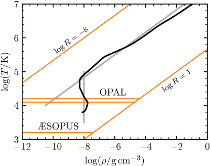
Figure 1: Opacity parameter space and table sources. The solid black line shows a representative profile from a stellar model. The grey lines indicate the slices of parameter space shown in Figures 2 and 3.

Figure 1 shows how these opacity sources cover the $T-\rho$ parameter space. We define the usual opacity parameter $\log R=\log(\rho/\mathrm{g\,cm^{-3}})-3\log(T/\mathrm{K})+18$. For comparison, Figure 1 in Paxton et al. (2011) illustrates default choices in MESA and Figure 1 in Weiss (1987) shows a similar visualization of the inputs used in that work. The grey lines show slices of parameter space where we will compare the different opacities.

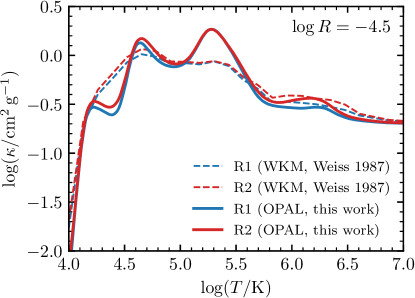
Figure 2: Comparison of opacities used in this work with those from Weiss (1987). The opacity is shown as a function of temperature at a constant value of $\log R$ (see diagonal grey line Figure 1). The more prominent Fe bump of more modern tables is particularly conspicuous. These tables have $Z=0.006$.

Figure 2 compares the OPAL opacities used in this work with the earlier opacities used in Weiss (1987) at temperatures $\log(T/\mathrm{K})\gtrsim 4.0$. A more detailed comparison of these opacity sources and an explanation of the differences is presented in Iglesias & Rogers (1993). We show this primarily to remind the reader of the significant difference at the location of the Fe opacity bump around $\log(T/\mathrm{K})\approx 5.2$.

Figure 3 compares different opacity sources at lower temperatures. The OPAL and ÆSOPUS tables agree well in their overlap region. We choose to locate the blend between the tables at $4.1\leq\log(T/\mathrm{K})\leq 4.2$, roughly in the middle of the overlap region. In this low temperature region, the WKM tables used in Weiss (1987) report systematically higher opacities, though they have similar shapes. The FA05 (Ferguson et al., 2005) opacities show significant differences because they assume a scaled-solar composition. We show them because this is what would be used by MESA by default if we had not included more suitable tables.

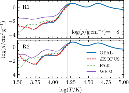
Figure 3: Comparison of opacities used in this work at lower temperatures. The opacity is shown as a function of temperature at a constant value of $\rho$ (see vertical grey line Figure 1). The vertical orange lines indicate the location of the temperature blending region. The OPAL and ÆSOPUS opacities agree well in this temperature range.

3.1 Atmosphere Boundary Conditions

Early studies of R CrB atmospheres were performed by Myerscough (1968) who included the effects of He (McDowell et al., 1966) and the ${\rm C}^{-}$ ion (Myerscough & McDowell, 1964, 1966) as well as by Schoenberner (1975). One-dimensional, line-blanketed model atmosphere calculations for these stars have been more recently computed by Asplund et al. (1997) and Asplund et al. (2000), but these are not available in a form that allows for easy incorporation in a stellar evolution code. Therefore, our outer boundary conditions come from atmosphere prescriptions that evaluate the Rosseland mean opacities in the same way as in the rest of the stellar model.

We emphasize that the improved treatment of CNO-enhanced, low-temperature opacities in this work should not be taken to indicate that the absolute effective temperatures of our models are particularly reliable. The simplifications inherent in 1D mixing length theory (Böhm-Vitense, 1958; Cox & Giuli, 1968) – whether in a stellar evolution or model atmosphere code – cannot reproduce the inherently 3D structure of convective envelopes, particularly in the super-adiabatically stratified outer layers. Promising future approaches include coupling of the results of 3D hydrodynamical simulations with 1D stellar evolution calculations (Jørgensen et al., 2018; Jørgensen & Weiss, 2019). However, details of where and how the boundary condition is applied can still lead to effective temperature ambiguities (e.g., Choi et al., 2018). We will illustrate the sensitivity to the outer boundary conditions in Section 4.2.

3.2 Comparison with other work

Recent work modeling R CrB stars has generally not taken these opacity effects into account. Menon et al. (2013) primarily use MESA with “Type 1” opacities (no C enhancement). They do some test runs using “Type 2” opacities, though these apply only at higher temperatures (i.e., the OPAL tables). They mention numerical difficulties, which they attribute to the physical instability of these envelopes. Likewise, Zhang et al. (2014) use the GS98 and FA05 tables. They also experience numerical difficulties that lead to small fluctuations in the luminosity. Similar fluctuations are apparent in the HR diagrams in Lauer et al. (2019). For the most part the models in the current work evolve smoothly when moving to the blue suggesting that some of these difficulties may have reflected a poor blend between the low and high temperature opacity tables. The exception is the models with the highest metallicity and highest luminosities, which are locally super-Eddington at the Fe opacity bump; such models continue to pose numerical challenges.

4 Helium Star Models

We first construct R CrB models via a modified evolution of helium stars. These are closely related to the homogeneous models of Weiss (1987). We begin the evolution from homogeneous models on the He ZAMS. We do not activate the predictive mixing capabilities described in Paxton et al. (2018). This may result in an underestimate of size of the convective core during the He MS, but we are not interested in the properties of the model during core burning. We let these models move into the shell burning phase and allow the CO cores to grow. When the envelope mass shrinks to 0.47 $\mathrm{M}_{\odot}$, we stop the models and instantaneously change the envelope composition. We then resume the evolution and continue until the model reaches $T_{\rm eff}=30\,\mathrm{kK}$ while moving to the blue. Only this latter portion of the evolution is shown in the paper. We do not include the effects of mass loss, so each model has a constant total mass. The primary goal of this section is to compare with past work and illustrate the sensitivity to various modeling assumptions.

4.1 Comparison with Weiss (1987)

As a first illustration of these models, Figure 4 shows 3 tracks in the HR diagram. These correspond to models of $Z=0.006$ He stars with an unmodified envelope composition and with compositions R1 and R2. These results are in general agreement with those in Weiss (1987). The models have similar luminosities during their redward and blueward evolution, with the MESA models being slightly $(\lesssim 0.1$ dex) warmer at their coolest point.

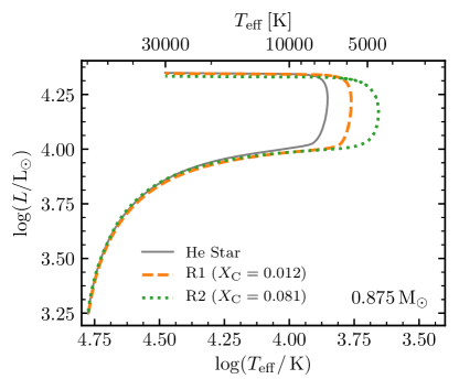
Figure 4: Evolution of He star models with varying envelope compositions. This reproduces the results of earlier work (cf. Figure 3b in Weiss, 1987).

4.2 Sensitivity to Outer Boundary Conditions

The effective temperatures of our models depend on the outer boundary condition, the mixing length parameter, and the opacities used in the model (see Section 3.1 for more discussion). Here we illustrate the shifts caused by different options. The illustrative model in used this subsection has $M=0.85\,\mathrm{\mathrm{M}_{\odot}}$, $Z=0.006$, and envelope composition R1.

Throughout, we default to using the MESA “simple photosphere” option, which uses a simple, constant grey opacity solution to the radiative diffusion equation (see Section 5.3 in Paxton et al., 2011). Figure 5 illustrates the results of other choices. We show the results with the “grey and kap” option, which is like the simple photosphere option, but with an additional iterative step to ensure that the pressure, temperature, and opacity at the surface are consistent. We also show the “Eddington grey” option, which integrates the $T-\tau$ relation of Eddington (1926). These options all agree at level of $\approx 100\,\mathrm{K}$.

Figure 5 also shows the effect of varying the mixing length parameter $\alpha_{\rm MLT}$. (The default value is $\alpha_{\rm MLT}=2$.) This shift is at the level of $\approx 1000\,\mathrm{K}$. This reflects the fact that as these He stars reach a substantial fraction of the Eddington luminosity, convection is becoming inefficient. This leads to density inversions in the outer layers and the radius to be particularly sensitive to $\alpha_{\rm MLT}$ (e.g., Joss et al., 1973; Sanyal et al., 2015).

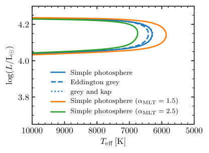
Figure 5: Effect of outer boundary condition and mixing length parameter on model effective temperatures.

4.3 Sensitivity to Composition and Opacities

Our fiducial composition has a base metallicity of $Z=0.006$. We adopt the CNO abundances of the majority R CrB population from Asplund et al. (2000). Their Table 6 gives, relative to the GS98 solar abundance pattern, a nitrogen enhancement factor $\log(f_{\rm N})=1.7$ and an oxygen enhancement factor $\log(f_{\rm O})=0.4$. We split the oxygen equally by mass between $\mathrm{{}^{16}O}$ and $\mathrm{{}^{18}O}$, though in the opacities there is no distinction between these isotopes.

The carbon abundances are somewhat less clear due to difficulty in modeling the C I lines (i.e., the carbon problem; Gustafsson & Asplund, 1996). Asplund et al. (2000) explore C/He number ratios in the range 0.1 to 10 per cent, finding ratios $\gtrsim 3\%$ are ruled out for the majority population. The EHe stars appear to have somewhat lower values with C/He $\approx 1\%$ (see Section 3.3.3 of Asplund et al., 2000, and references therein). Our fiducial carbon enhancement factor is $\log(f_{\rm C})=1.2$, corresponding to a carbon mass fraction of $\approx 0.04$, and hence a number ratio of $\approx 1\%$.

Figure 6 illustrates the effect of varying the metallicity at a fixed mass of $0.875\,\mathrm{\mathrm{M}_{\odot}}$. All models have the exact same composition in terms of He and CNO elements, but the base metallicity of the opacity tables is varied. This illustrates the influence of the Fe-bump on the radius of the envelope. The $Z=0.02$ model experiences numerical problems. As the opacity and/or luminosity rise, convection becomes increasing inefficient, requiring an increasingly super-adiabatic temperature gradient to transport the energy. As a result a steep entropy gradient develops at the base of the convection zone. Resolving this feature and its Lagrangian movement (as the envelope mass changes due to the He shell burning at the base) requires short timesteps and can also trigger numerical convergence issues. (See the MESA He star models of Hall & Jeffery 2018 for another example of this issue). These could be circumvented by artificially increasing the efficiency of convection (e.g., using the MLT++ prescription; Paxton et al., 2013), though that does not necessarily produce reliable radius estimates.

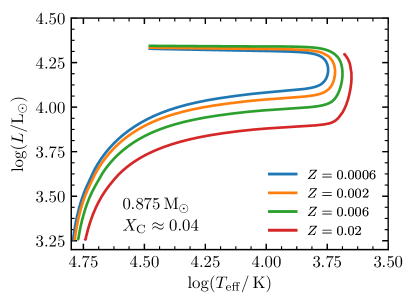
Figure 6: Effect of varying base metallicity at fixed mass and envelope composition. The highest metallicity model experiences numerical issues in the outer layers before evolving back to the blue.

Figure 7 shows the effect of changing the envelope carbon fraction at a fixed base metallicity of $Z=0.006$. This is a similar exercise as Figure 4, except that we also show models when the scaled-solar FA05 opacities are used instead of the CNO-enhanced ÆSOPUS opacities. This illustrates the level of difference between previous models using versions of MESA that only had scaled-solar low-temperature opacity options available. Models are generally $\approx 500\,\mathrm{K}$ warmer.

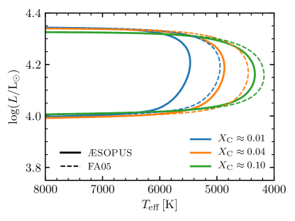
Figure 7: Change in effective temperature when varying surface carbon fraction at a fixed base metallicity of $Z=0.006$. The solid lines show the results using the CNO-enhanced ÆSOPUS opacities. The thin dashed lines show the calculations, but using the scaled-solar FA05 opacities.

5 Merger Models

The He star models presented in Section 4 are a simple way to construct an R CrB-like object. However, their configuration may be somewhat different than that realized in a WD merger. In particular, Iben (1990) emphasizes the importance of the thermal state of the core. In the WD merger case, one may expect the CO WD that forms the core to be more degenerate than the CO core created within the He star at the conclusion of He core burning. Therefore, in this section, we construct models more directly motivated by the post-merger configuration of a double WD merger. We initialize MESA models with cold CO cores and high entropy He-rich envelopes and discuss their evolution.

5.1 Detailed Merger Model

Schwab et al. (2012) performed multi-dimensional simulations of the viscous phase of the merger (using an $\alpha$-viscosity prescription), beginning from the output of SPH simulations of the dynamical phase of the merger (Dan et al., 2011) and covering the hours-long phase where the rotationally-supported disc transitions into a spherical, thermally-supported envelope (Shen et al., 2012). We focus on the model ZP4, which is the merger of an $0.3\,\mathrm{\mathrm{M}_{\odot}}$ He WD with an $0.6\,\mathrm{\mathrm{M}_{\odot}}$ CO WD. A small amount of material is lost during the merger and the remnant has a total mass $0.88\,\mathrm{\mathrm{M}_{\odot}}$.

In the same manner as Schwab et al. (2016), we take the final output of the Schwab et al. (2012) calculation, spherically-average the entropy and composition profiles, and then generate MESA models that approximately match these profiles. The initial state of this model is shown in Figure 8. We do not include the effects of rotation, though the outer layers of the model do still have some rotational support, which is the primary source of the disagreement between the spherical averages and the MESA model at $q\gtrsim 0.9$. Additionally, in the cool outer layers $(\log(T/\mathrm{K})\lesssim 7)$, there is a mismatch in the equation of state between the hydrodynamics calculations and MESA. The hydrodynamics calculations use the Helmholtz EOS (Timmes & Swesty, 2000) assuming full ionization, whereas the MESA EOS accounts for ionization via the use of OPAL (Rogers et al., 1996) and PTEH (Pols et al., 1995). Therefore, the detailed thermal structure of the very outer parts of the MESA model is unlikely to be particularly reliable. However, the region around the temperature peak where most of the thermal energy resides is a good match.

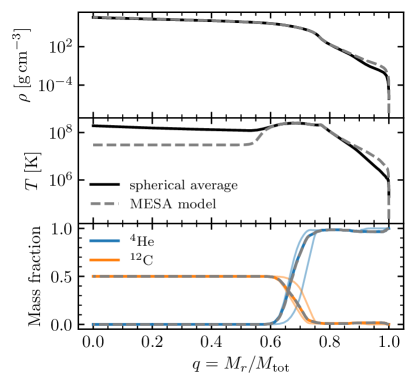
Figure 8: Comparison of density, temperature, and composition profiles between spherical averages taken at the end of the hydrodynamic calculations of the viscous disc phase (model ZP4 from Schwab et al., 2012) and the initial MESA model. In the lower panel, the thin lines indicate the composition profiles taken along polar and equatorial slices.

As noted in Schwab et al. (2012), while the overall remnant in this case is spherical, the composition profile varies with polar angle. We illustrate this with the thin lines in the lower panel of Figure 8, which show the composition profiles along polar and equatorial slices. The spherical averaging necessary to construct the 1D MESA models leads to some unavoidable chemical mixing in the interface region.

In the models of Dan et al. (2011) the He WDs are composed of $\mathrm{{}^{4}He}$ (and the CO WDs have equal mass fractions of $\mathrm{{}^{12}C}$ and $\mathrm{{}^{16}O}$). The hydrodynamic evolution uses a minimal (7 isotope) nuclear network. Likewise, the calculations in Schwab et al. (2012) use a small network to track the energy release from He burning. This means that these calculations contain little information about the nucleosynthesis in the merger and its immediate aftermath. In particular, directly confronting the observed surface abundances of R CrB stars requires a more detailed chemical model of the He WD and a larger nuclear network to follow the key chemical conversions (e.g., CNO cycling from $\mathrm{{}^{1}H}$, $\mathrm{{}^{7}Li}$ from $\mathrm{{}^{3}He}$, $\mathrm{{}^{18}O}$ from $\mathrm{{}^{14}N}$). Work such as Lauer et al. (2019) performs MESA calculations using a larger nuclear network and other work post-processes with yet larger ones (Longland et al., 2012; Menon et al., 2013). Here, given the limitations of our modeling approach, we choose not to focus on the nucleosynthesis.

5.2 Schematic Merger Models

We also generate some models that are not based directly on the result of merger calculations, but instead schematically reproduce configurations with a cold core and thermally-supported envelope. Given the uncertainties in the merger modeling, these help to provide a sense of which evolutionary features are robust. Because they are simple to construct, they also allow for rapid exploration of the parameter space.

We pick a CO core mass and a He envelope mass and assume a sharp core-envelope boundary. For simplicity, all models have the same core temperature ($T=3\times 10^{7}\,\mathrm{K}$). We initialize the envelope with a constant specific entropy. By default, we assume $s=10^{9}\,\mathrm{\rm erg\,g^{-1}\,K^{-1}}$. This approach is similar to that applied in Shen et al. (2012) and the relaxation procedure used was adapted from publicly-available code (Shen, 2015). The core composition is equal mass fractions of $\mathrm{{}^{12}C}$ and $\mathrm{{}^{16}O}$. The envelope initially has the same fiducial composition described in Section 4.3.

Figure 9 shows the initial temperature and density profile for models with different envelope entropies. Compared with the model ZP4 from Section 5.1, the peak temperature is similar, though generally at lower density in the schematic models (SD and SL).

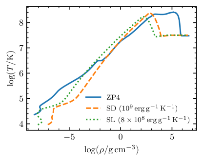
Figure 9: Initial temperature-density profiles of merger models. Model ZP4 is the detailed merger model described in Section 5.1. Model SD is the schematic merger model described in Section 5.2 for a $0.3\,\mathrm{\mathrm{M}_{\odot}}$ He WD and $0.6\,\mathrm{\mathrm{M}_{\odot}}$ CO WD. Model SL is the same as model SD, but with a lower specific envelope entropy of $s=8\times 10^{8}\,\mathrm{\rm erg\,g^{-1}\,K^{-1}}$.

5.3 Comparative Evolution

The primary qualitative difference between these models and the He star models of Section 4 lies in the early time evolution. The merged remnant is far from thermal equilibrium. The base of the envelope must first set up the steady He-burning shell and then the rest of the envelope adjusts to this input luminosity. The post merger configuration is generally compact, and so initially the thermal energy deposited in the merger and released from nuclear burning goes into work leading to expansion. As a result, the objects begin at relatively lower luminosities that then increase as they move towards the steady He shell burning configuration.

Figure 10 shows the early post-merger evolution of the models shown in Figure 9. As a consequence of the differences in the initial models, the behavior is different at first. However, by the time they reach $\log(L/\mathrm{L}_{\odot})\gtrsim 2.5$ all models are similar. The tracks continue until $L\approx L_{\rm He}$ (surface luminosity is approximately nuclear luminosity from He burning). The amount of time elapsed in the simulation is indicated in the legend, ranging from $300\,\mathrm{yr}$ to $900\,\mathrm{yr}$. We suspect that the longer time corresponding the ZP4 model is more physically realistic. In the SPH merger models of Dan et al. (2014), a $q=0.5$ merger has only about half its mass in the cold core (with the remainder roughly equally distributed between a disk and hot envelope). In contrast, our simple schematic merger models have the entire mass of the primary (i.e., two-thirds of the total mass) in their cold cores. The schematic merger models thus represent an extreme limit and likely have systematically shorter thermal times from the temperature peak to the surface than models based on merger calculations where the outer layers of the primary have been strongly heated during the merger.

The existence of this thermal reconfiguration phase is one of the hallmarks of double WD mergers. It is not present in the early evolution of models coming from homogeneous He stars (e.g., Section 4; Weiss, 1987; Menon et al., 2013). The Lauer et al. (2019) models, constructed similarly to the schematic models, also show this early brightening phase. In the Zhang et al. (2014) destroyed disc models this segment of the evolution lasts $\approx 500\,\mathrm{yr}$ (see their Figure 18).

Given R CrB lifetimes $\sim 5\times 10^{4}\,\mathrm{yr}$, the relative duration of this phase is $\sim 1\%$. The galactic R CrB stars number in the hundreds (e.g., Tisserand et al., 2018). The relative duration suggests the presence of at least a few objects in this pre-R CrB phase. These objects may not yet exhibit the complex photometric behavior characteristic of the R CrB stars, and so may not be classified as such. These pre-R CrB objects will be gradually growing brighter and cooler on timescales comparable to the baseline covered by historical photometric catalogs. They also have likely not yet shed significant quantities of dusty material and so should have different circumstellar environments from objects that are settled in the R CrB phase.

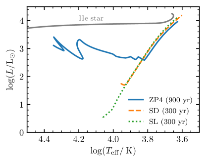
Figure 10: Evolution in the HR diagram shortly after merger. Indicated times are the duration from the start of the calculation until the surface luminosity and the luminosity from He burning are first equal. The grey line shows the qualitatively different evolutionary track from a homogeneous He star model.

6 Effects of Mass Loss

Mass loss plays an important role in R CrB evolution. Dusty shells, with dust masses up to $10^{-3}\,\mathrm{\mathrm{M}_{\odot}}$, exist in the surroundings of R CrB stars and are interpreted to have formed during the R CrB phase (Montiel et al., 2015, 2018). The terminal velocities of R CrB star winds are $v_{\infty}\approx 300\,\mathrm{\mathrm{km\,s^{-1}}}$ (Clayton et al., 2003, 2013). Note that this is $\gtrsim 10$ times greater than typical carbon-rich AGB wind velocities (e.g., Groenewegen et al., 1998). Recent evolutionary models of R CrB stars have adopted the AGB wind prescription of Bloecker (1995), with efficiency factors $\eta\approx 0.02$ (Menon et al., 2013; Zhang et al., 2014; Lauer et al., 2019). Typically mass loss rates are then $\sim 10^{-6}-10^{-5}\,\mathrm{\mathrm{M}_{\odot}\,\mathrm{yr}^{-1}}$.

The application of existing mass loss prescriptions to the R CrB stars comes with significant caveats. The R CrB stars have different envelope compositions (H-deficient, C-rich) than AGB stars (normal H, often O-rich). Their pulsation periods are also shorter ($\lesssim 100\,\mathrm{d}$) than those of the long-period variables that motivate prescriptions like that of Bloecker (1995). Even if AGB mass loss were a solved problem, the solutions would not be directly applicable to the R CrB stars. Nonetheless, these existing prescriptions provide a convenient initial guess for exploration.

The merger creates a He envelope of $\approx 0.3\,\mathrm{\mathrm{M}_{\odot}}$ on a CO core. Then, the lifetime of the R CrB phase is given by the timescale to exhaust this envelope as material is added to the CO core through He-burning $(\dot{M}_{\rm He})$ and removed from the star through winds $(\dot{M}_{\rm wind})$. First, note $\dot{M}_{\rm He}=L/Q_{\rm He}$ and $L$ is a strong function of the CO core mass $M_{\rm core}$. For example, $d\ln L/d\ln\mathrm{M}_{\rm core}\approx 5$ for $\mathrm{M}_{\rm core}\approx 0.6\,\mathrm{\mathrm{M}_{\odot}}$ (Jeffery, 1988). Second, note that $\dot{M}_{\rm wind}$ also likely increases with increasing $L$. Thus, the envelope is exhausted more rapidly by both processes as the core grows, meaning that more time is spent at lower core masses in any given model.

If the wind mass loss rates grow strongly with $L$—the Bloecker (1995) prescription has $\dot{M}\propto L^{3.7}$—then this effectively creates a critical core mass defined by the point where $\dot{M}_{\rm wind}\approx\dot{M}_{\rm He}$. For initial core masses below this critical mass, the core can grow. But once it reaches the critical mass (or if the initial core mass is above it), the large luminosity causes the envelope to be rapidly shed. Therefore, though there can be a significant range in the initial total mass of the remnant, this may be erased by mass loss.

The wind velocity implies an upper limit to the mass loss rate of

$$\dot{M}_{\rm max}\approx\frac{2L}{v_{\infty}^{2}}\sim 10^{-3}\,\mathrm{\mathrm{M}_{\odot}\,\mathrm{yr}^{-1}}\left(\frac{L}{10^{4}\,\mathrm{\mathrm{L}_{\odot}}}\right)\left(\frac{v_{\infty}}{300\,\mathrm{\mathrm{km\,s^{-1}}}}\right)^{-2}~{},$$ (1)

on energetic grounds. Comparing the wind specific kinetic energy to the specific energy of He-burning, we see

$$v_{\infty}^{2}\approx 10^{15}\,\mathrm{erg\,g^{-1}}\ll Q_{\rm He}\approx 7\times 10^{17}\,\mathrm{erg\,g^{-1}}~{}.$$ (2)

The ad hoc assumption that $\dot{M}=f\dot{M}_{\rm max}$ (with a constant value of $f$) provides a simple expression that we will use to draw a contrast with the Bloecker (1995) prescription and its much steeper $L$ dependence. Under this assumption, the growth of the core is

$$\Delta M=M_{\rm He}\left(1+\frac{2fQ_{\rm He}}{v_{\infty}^{2}}\right)^{-1}~{}.$$ (3)

Then for $f\gtrsim v_{\infty}^{2}/(2Q_{\rm He})\sim 10^{-3}$, only a small amount of the He will be added to the CO core and the rest will be lost from the star.

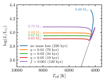
Figure 11: Evolutionary dependence on mass loss rate. Total masses are indicated at the end of each track. Lifetimes are indicated in the legend. The thin portion of the track is the early thermal adjustment phase (shown in more detail in Figure 10) and is not included in the stated lifetime. Models labeled with $\eta$ values use a Bloecker (1995) wind with that scaling factor. The model labeled with an $f$ value uses a wind that with that constant fraction of the maximum given by Equation (1).

Figure 11 shows initial model ZP4 evolved with the Bloecker (1995) wind prescription in MESA using a range of efficiency factors $\eta$. Once the He envelope shrinks to $\approx 0.05\,\mathrm{\mathrm{M}_{\odot}}$ the models begin to evolve to the blue. The case without mass loss reaches a near-Eddington luminosity and we have halted this model at a CO core mass $\approx 0.8\,\mathrm{\mathrm{M}_{\odot}}$, when the timestep becomes severely limited (see Section 4.3 for a discussion of this issue). For the models including mass loss, the total mass does not have a strong dependence on $\eta$, and they evolve to the blue with masses $\approx 0.65-0.70\,\mathrm{\mathrm{M}_{\odot}}$. However, the lifetime is more sensitive, with the factor of 5 variation in $\eta$ giving a factor of $\approx 3$ change in lifetime. These lifetimes and masses are consistent with past work. The models of Zhang et al. (2014) typically spend $50–70\,\mathrm{kyr}$ in the R CrB phase; the models of Lauer et al. (2019) spend $\sim 10^{5}\,\mathrm{yr}$. Similarly, both works show the total masses being reduced to $\approx 0.7\,\mathrm{\mathrm{M}_{\odot}}$. The model in Figure 11 with $f=0.001$ illustrates a different prescription giving a similar final mass but significantly different lifetime.

Figure 14 shows the total mass of each of a grid of schematic merger models (all with CO primaries less massive than $0.7\,\mathrm{\mathrm{M}_{\odot}}$) at a time after they have evolved to the blue (reached $T_{\rm eff}=10^{4}\,\mathrm{K}$). We compare two mass loss prescriptions: the top plot (a) uses the Bloecker (1995) wind with $\eta=0.02$; the bottom plot (b) uses $\dot{M}=f\dot{M}_{\rm max}$ with $f=0.001$. The systems have a range of initial total masses $0.7-1.05\,\mathrm{\mathrm{M}_{\odot}}$. In plot (a), all leave the R CrB phase with total masses in the range $\approx 0.6-0.7\,\mathrm{\mathrm{M}_{\odot}}$. In plot (b), the systems have masses $\approx 0.65-0.8\,\mathrm{\mathrm{M}_{\odot}}$, more massive on average and with a slightly wider mass range than those in plot (a). This is as expected given the mass loss rates in plot (b) increase less rapidly as $L$ grows. Though the exact numbers will depend on the implemented prescription, this illustrates the inevitable effect of mass loss to concentrate remnants toward lower total masses.

6.1 Implications for R CrB descendants

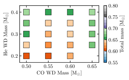
Figure 12: (a) Bloecker (1995) wind using $\eta=0.02$.

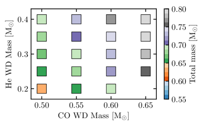
Figure 13: (b) Wind with $\dot{M}=f\dot{M}_{\rm max}$ using $f=0.001$.

Figure 14: Total mass at the end of the R CrB phase when models reached $T_{\rm eff}=10^{4}\,\mathrm{K}$.

The likely direct decedents of the R CrB stars are the extreme He (EHe) stars (e.g., Pandey et al., 2001; Jeffery, 2008), in particular the portion of the population that lies relatively close to the Eddington luminosity. The mass-luminosity relationship for EHe stars (Saio, 1988; Jeffery, 1988) provides an opportunity to probe their masses, which for some objects may be aided by improved distances from Gaia (Gaia Collaboration et al., 2016). The presence of radial pulsations in these objects provides additional information and Saio & Jeffery (1988) and Jeffery et al. (2001) use spectroscopic and pulsational methods to measure masses. In a number of systems, multiple methods are in agreement, leading to EHe star masses $\approx 0.8-0.95\,\mathrm{\mathrm{M}_{\odot}}$ (though with significant uncertainties). These masses are in tension with the lower masses of the models shown in Figure 14. This may indicate that the amount of mass lost is overestimated in these models.

Alternatively, even with this mass loss, an object with $\gtrsim 0.7\,\mathrm{\mathrm{M}_{\odot}}$ could indicate a CO WD primary $\gtrsim 0.7\,\mathrm{\mathrm{M}_{\odot}}$, since the material that is shed is material from the He WD secondary. However, these higher mass CO WD systems may be near the lower limit for the occurrence of a detonation in the He accretion stream during the merger itself (Guillochon et al., 2010), which can then trigger the detonation of the CO core. (For a summary of this double detonation scenario in the context of Type Ia SNe, see Shen et al. 2018). Detonations of CO WDs in the mass range $0.7-0.85\,\mathrm{\mathrm{M}_{\odot}}$ would not produce the $\mathrm{{}^{56}Ni}$ necessary to power a Type Ia SN, but would primarily synthesize intermediate mass elements (Polin et al., 2019). This would still likely result in the destruction of the system (and hence not the formation of an R CrB star). Therefore, it may be that mergers with CO primaries $\gtrsim 0.7\,\mathrm{\mathrm{M}_{\odot}}$ and He-rich secondaries are catastrophically destroyed during the merger process. This picture could also fit with the suggestion by Staff et al. (2018) that He buffer layers are required to reproduce the $\mathrm{{}^{18}O}$/$\mathrm{{}^{16}O}$ ratio, since CO WDs up to around $0.7\,\mathrm{\mathrm{M}_{\odot}}$ maintain significant surface He layers (e.g., Zenati et al., 2019).

The relative duration of the EHe and R CrB phases is particularly sensitive to the adopted mass loss rates. Less mass loss implies a longer R CrB lifetime and more core growth. But then a higher core mass implies a shorter EHe lifetime, as the residual He layer is more rapidly exhausted at higher luminosity (Saio, 1988).

Figure 15 shows the HR and Kiel diagrams for models using Bloecker (1995) winds with $\eta=0.002$ and $\eta=0.02$. The model with the lower mass loss rate spends approximately three times as long in a R CrB phase and becomes $0.07\,\mathrm{\mathrm{M}_{\odot}}$ more massive. The dots, spaced each 10 kyr along the evolutionary tracks, show that this more massive remnant evolves blueward approximately twice as fast. Thus, these two choices for the mass loss (which give final remnant masses within $\approx 10$ %) are different by a factor of $\approx 6$ in the ratio of the predicted R CrB-to-EHe lifetimes.

The models continue to move blueward throughout the EHe phase and evolve to higher surface gravity where they appear as sdO stars. For reference, Figure 15 also shows an sdO track of a He WD + He WD merger model from Schwab (2018). As the models approach their maximum effective temperature, they appear as O(He) stars (e.g., Rauch et al., 2008; Reindl et al., 2014), before finally moving onto the WD cooling track. Though we do not pursue it here, there is potential to constrain and refine the models by exploiting the connections between R CrB populations and their blue descendants.

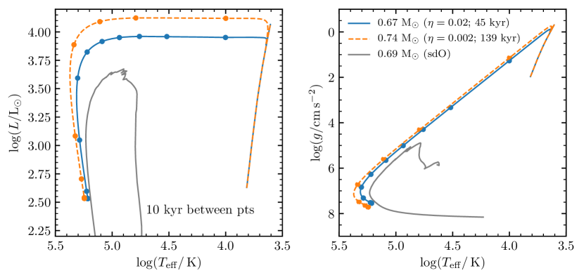
Figure 15: HR diagram (left panel) and Kiel diagram (right panel) for two models (colored lines) using Bloecker (1995) mass loss rates with different $\eta$. The approximate time in the R CrB phase is indicated in the right legend. Beginning when the models reach $T_{\rm eff}=10^{4}\,\mathrm{K}$, dots along the evolutionary tracks are spaced in 10 kyr intervals. The grey track shows a He + He WD merger model (M07 from Schwab, 2018) that has a similar final mass as the other models but never had a giant phase.

6.2 Implications for single WDs

Eventually, the remnants of these double WD mergers will evolve into single WDs. The detection of single WDs with relatively short cooling ages but kinematics consistent with ages much longer than the single-star evolutionary timescale at their mass probe the contribution of double WD mergers to the single WD population (e.g., Wegg & Phinney, 2012). The hot DQ WDs (Dufour et al., 2008) have been speculated to show the kinematic signatures associated with mergers (Dunlap & Clemens, 2015) as have some other massive DQs (Cheng et al., 2019).

Immediately after the merger, the total mass of the remnant is approximately the sum of the component masses, with only $\sim 10^{-3}\,\mathrm{\mathrm{M}_{\odot}}$ being ejected during the merger itself (e.g., Lorén-Aguilar et al., 2009). The mass lost during the subsequent evolution to a single WD then seems likely to be the dominant effect in setting the final mass. Different post-merger evolutionary pathways imprint themselves on the mapping from the total mass distribution of merging WDs to the mass distribution of single WDs coming from merged WDs.

Double He WD mergers evolve through a hot subdwarf phase (e.g., Zhang & Jeffery, 2012b) that does not result in significant wind mass loss. Some angular momentum must be shed in order for the remnant to reach a He core burning configuration, but this can be achieved while losing only $\sim 10^{-2}\,\mathrm{\mathrm{M}_{\odot}}$ (Gourgouliatos & Jeffery, 2006; Schwab, 2018).

As discussed earlier, He WD + CO WD mergers that undergo an R CrB phase are predicted to lose $\sim 10^{-1}\,\mathrm{\mathrm{M}_{\odot}}$, with initially more massive systems preferentially losing more mass. Moreover, if systems with higher mass CO WD primaries ($\gtrsim 0.7\,\mathrm{\mathrm{M}_{\odot}}$) are destroyed during the merger process as a result of double detonations, this would further remove systems with higher total masses from the pool that will leave behind single WDs. Together, these effects might lead to an enhancement of single WDs formed by double WD mergers around the masses of the EHe stars and a relative scarcity immediately above that.

At yet higher masses ($\approx 1.1\,\mathrm{\mathrm{M}_{\odot}}$), double CO WD mergers would begin to leave single WD remnants again. These more massive merger remnants may also experience mass loss and hence a reduction in their total masses. However, since they do not set up long-lived, shell-powered burning giant structures (e.g., Nomoto & Iben, 1985), the mass loss may be qualitatively different and less extreme than the R CrB stars.

7 Summary & Conclusions

We use the MESA stellar evolution code to construct evolutionary models of stars that reach an R CrB-like phase. We incorporated opacities from ÆSOPUS (Marigo & Aringer, 2009) appropriate for the cool, H-deficient, CNO-enhanced photospheres of these stars. We use these to discuss some of the model variations expected as a result of variations in metallicity, envelope composition, and the modeling of convection.

We construct models via the evolution of He stars (reproducing Weiss, 1987). We also construct two types of models of the remnants of double WD mergers: one is a MESA realization of the end state of the merger calculation of Schwab et al. (2012); the other engineers models that have a cold CO core and high entropy He envelope, schematically reproducing the post-merger structure. We emphasize that models originating from double WD merger scenarios have a thermal reconfiguration phase that can last up to $\approx 1\,\mathrm{kyr}$ post merger. Some galactic objects should be in this phase and we suggest they could be distinguished by their lower luminosities, secular brightening, and by the fact that their circumstellar environments should not yet have accumulated significant dusty shells from mass loss during the R CrB phase.

We illustrate, in agreement with the results of past work (Zhang et al., 2014; Lauer et al., 2019), that R CrB models that include mass loss based on AGB prescriptions like that of Bloecker (1995) typically leave the R CrB phase with total masses $\approx 0.7\,\mathrm{\mathrm{M}_{\odot}}$. When the mass loss rates scale with $L$, the steep core mass-luminosity relationship for He giants implies convergent evolution in mass, where the initially lower mass CO WDs grow through He shell burning but higher mass ones do not. This implies that the descendants of most R CrB stars should have a relatively narrow range in mass ($\approx 0.1\,\mathrm{\mathrm{M}_{\odot}}$), substantially narrower than the range in total mass of the systems that form them. Moreover, if double detonations (e.g., Guillochon et al., 2010; Shen et al., 2018) are common in mergers involving CO WDs with masses $\gtrsim 0.7\,\mathrm{\mathrm{M}_{\odot}}$, then this would remove the possibility of forming R CrB stars with CO cores above this mass. If this is true, such a limit should be reflected in the masses and luminosities of extreme He stars and the masses of the single WDs that they eventually become.

Connecting populations of double WD systems (whether observed or from population synthesis) to the observed numbers of R CrB stars requires accurate lifetime estimates. In turn, accurate mass loss prescriptions are required for accurate lifetime estimates; our R CrB model lifetimes vary by a factor of a few, depending on the assumed prescription. As also noted by Zhang et al. (2014), more theoretical work that unifies the periodic dust formation that is the R CrB phenomenon itself with the long-term average mass loss is desirable. In the future, this would enable models to move beyond the application of existing AGB mass loss rates to these H-deficient stars.

References

- Asplund et al. (1997) Asplund, M., Gustafsson, B., Kiselman, D., & Eriksson, K. 1997, A&A, 318, 521
- Asplund et al. (2000) Asplund, M., Gustafsson, B., Lambert, D. L., & Rao, N. K. 2000, A&A, 353, 287
- Biermann & Kippenhahn (1971) Biermann, P., & Kippenhahn, R. 1971, A&A, 14, 32
- Bloecker (1995) Bloecker, T. 1995, A&A, 297, 727
- Böhm-Vitense (1958) Böhm-Vitense, E. 1958, ZAp, 46, 108
- Cheng et al. (2019) Cheng, S., Cummings, J., & Ménard, B. 2019, arXiv e-prints, arXiv:1905.12710. https://arxiv.org/abs/1905.12710
- Choi et al. (2018) Choi, J., Dotter, A., Conroy, C., & Ting, Y.-S. 2018, ApJ, 860, 131, doi: 10.3847/1538-4357/aac435
- Clayton (1996) Clayton, G. C. 1996, PASP, 108, 225, doi: 10.1086/133715
- Clayton (2012) —. 2012, Journal of the American Association of Variable Star Observers (JAAVSO), 40, 539. https://arxiv.org/abs/1206.3448
- Clayton et al. (2003) Clayton, G. C., Geballe, T. R., & Bianchi, L. 2003, ApJ, 595, 412, doi: 10.1086/377336
- Clayton et al. (2007) Clayton, G. C., Geballe, T. R., Herwig, F., Fryer, C., & Asplund, M. 2007, ApJ, 662, 1220, doi: 10.1086/518307
- Clayton et al. (2013) Clayton, G. C., Geballe, T. R., & Zhang, W. 2013, AJ, 146, 23, doi: 10.1088/0004-6256/146/2/23
- Cox & Giuli (1968) Cox, J. P., & Giuli, R. T. 1968, Principles of stellar structure
- Dan et al. (2014) Dan, M., Rosswog, S., Brüggen, M., & Podsiadlowski, P. 2014, MNRAS, 438, 14, doi: 10.1093/mnras/stt1766
- Dan et al. (2011) Dan, M., Rosswog, S., Guillochon, J., & Ramirez-Ruiz, E. 2011, ApJ, 737, 89, doi: 10.1088/0004-637X/737/2/89
- Dufour et al. (2008) Dufour, P., Fontaine, G., Liebert, J., Schmidt, G. D., & Behara, N. 2008, ApJ, 683, 978, doi: 10.1086/589855
- Dunlap & Clemens (2015) Dunlap, B. H., & Clemens, J. C. 2015, in Astronomical Society of the Pacific Conference Series, Vol. 493, 19th European Workshop on White Dwarfs, ed. P. Dufour, P. Bergeron, & G. Fontaine, 547
- Eddington (1926) Eddington, A. S. 1926, The Internal Constitution of the Stars
- Ferguson et al. (2005) Ferguson, J. W., Alexander, D. R., Allard, F., et al. 2005, ApJ, 623, 585, doi: 10.1086/428642
- Gaia Collaboration et al. (2016) Gaia Collaboration, Prusti, T., de Bruijne, J. H. J., et al. 2016, A&A, 595, A1, doi: 10.1051/0004-6361/201629272
- Gourgouliatos & Jeffery (2006) Gourgouliatos, K. N., & Jeffery, C. S. 2006, MNRAS, 371, 1381, doi: 10.1111/j.1365-2966.2006.10780.x
- Grevesse & Sauval (1998) Grevesse, N., & Sauval, A. J. 1998, Space Sci. Rev., 85, 161, doi: 10.1023/A:1005161325181
- Groenewegen et al. (1998) Groenewegen, M. A. T., Whitelock, P. A., Smith, C. H., & Kerschbaum, F. 1998, MNRAS, 293, 18, doi: 10.1046/j.1365-8711.1998.01113.x
- Guillochon et al. (2010) Guillochon, J., Dan, M., Ramirez-Ruiz, E., & Rosswog, S. 2010, ApJ, 709, L64, doi: 10.1088/2041-8205/709/1/L64
- Gustafsson & Asplund (1996) Gustafsson, B., & Asplund, M. 1996, in Astronomical Society of the Pacific Conference Series, Vol. 96, Hydrogen Deficient Stars, ed. C. S. Jeffery & U. Heber, 27
- Hall & Jeffery (2018) Hall, P. D., & Jeffery, C. S. 2018, MNRAS, 475, 3889, doi: 10.1093/mnras/sty055
- Huebner et al. (1977) Huebner, W. F., Merts, A., Magee Jr, N., & Argo, M. 1977, Astrophysical opacity library, Tech. Rep. LA-6760-M, Los Alamos Scientific Lab.
- Hunter (2007) Hunter, J. D. 2007, Computing In Science & Engineering, 9, 90
- Iben (1990) Iben, Jr., I. 1990, ApJ, 353, 215, doi: 10.1086/168609
- Iben & Tutukov (1989) Iben, Jr., I., & Tutukov, A. V. 1989, ApJ, 342, 430, doi: 10.1086/167603
- Iglesias & Rogers (1993) Iglesias, C. A., & Rogers, F. J. 1993, ApJ, 412, 752, doi: 10.1086/172958
- Iglesias & Rogers (1996) —. 1996, ApJ, 464, 943, doi: 10.1086/177381
- Jeffery (1988) Jeffery, C. S. 1988, MNRAS, 235, 1287, doi: 10.1093/mnras/235.4.1287
- Jeffery (2008) Jeffery, C. S. 2008, in Astronomical Society of the Pacific Conference Series, Vol. 391, Hydrogen-Deficient Stars, ed. A. Werner & T. Rauch, 53
- Jeffery (2017) —. 2017, MNRAS, 470, 3557, doi: 10.1093/mnras/stx1442
- Jeffery et al. (2011) Jeffery, C. S., Karakas, A. I., & Saio, H. 2011, MNRAS, 414, 3599, doi: 10.1111/j.1365-2966.2011.18667.x
- Jeffery et al. (2001) Jeffery, C. S., Starling, R. L. C., Hill, P. W., & Pollacco, D. 2001, MNRAS, 321, 111, doi: 10.1046/j.1365-8711.2001.03992.x
- Jørgensen et al. (2018) Jørgensen, A. C. S., Mosumgaard, J. R., Weiss, A., Silva Aguirre, V., & Christensen-Dalsgaard, J. 2018, MNRAS, 481, L35, doi: 10.1093/mnrasl/sly152
- Jørgensen & Weiss (2019) Jørgensen, A. C. S., & Weiss, A. 2019, MNRAS, 488, 3463, doi: 10.1093/mnras/stz1980
- Joss et al. (1973) Joss, P. C., Salpeter, E. E., & Ostriker, J. P. 1973, ApJ, 181, 429, doi: 10.1086/152060
- Karakas et al. (2015) Karakas, A. I., Ruiter, A. J., & Hampel, M. 2015, ApJ, 809, 184, doi: 10.1088/0004-637X/809/2/184
- Lauer et al. (2019) Lauer, A., Chatzopoulos, E., Clayton, G. C., Frank, J., & Marcello, D. C. 2019, MNRAS, 488, 438, doi: 10.1093/mnras/stz1732
- Longland et al. (2012) Longland, R., Lorén-Aguilar, P., José, J., García-Berro, E., & Althaus, L. G. 2012, A&A, 542, A117, doi: 10.1051/0004-6361/201219289
- Longland et al. (2011) Longland, R., Lorén-Aguilar, P., José, J., et al. 2011, ApJ, 737, L34, doi: 10.1088/2041-8205/737/2/L34
- Lorén-Aguilar et al. (2009) Lorén-Aguilar, P., Isern, J., & García-Berro, E. 2009, A&A, 500, 1193, doi: 10.1051/0004-6361/200811060
- Marigo & Aringer (2009) Marigo, P., & Aringer, B. 2009, A&A, 508, 1539, doi: 10.1051/0004-6361/200912598
- McDowell et al. (1966) McDowell, M. R. C., Williamson, J. H., & Myerscough, V. P. 1966, ApJ, 144, 827, doi: 10.1086/148665
- Menon et al. (2013) Menon, A., Herwig, F., Denissenkov, P. A., et al. 2013, ApJ, 772, 59, doi: 10.1088/0004-637X/772/1/59
- Menon et al. (2019) Menon, A., Karakas, A. I., Lugaro, M., Doherty, C. L., & Ritter, C. 2019, MNRAS, 482, 2320, doi: 10.1093/mnras/sty2606
- Montiel et al. (2015) Montiel, E. J., Clayton, G. C., Marcello, D. C., & Lockman, F. J. 2015, AJ, 150, 14, doi: 10.1088/0004-6256/150/1/14
- Montiel et al. (2018) Montiel, E. J., Clayton, G. C., Sugerman, B. E. K., et al. 2018, AJ, 156, 148, doi: 10.3847/1538-3881/aad772
- Myerscough (1968) Myerscough, V. P. 1968, ApJ, 153, 421, doi: 10.1086/149677
- Myerscough & McDowell (1964) Myerscough, V. P., & McDowell, M. R. C. 1964, MNRAS, 128, 287
- Myerscough & McDowell (1966) —. 1966, MNRAS, 132, 457
- Nomoto & Iben (1985) Nomoto, K., & Iben, Jr., I. 1985, ApJ, 297, 531, doi: 10.1086/163547
- Paczyński (1971) Paczyński, B. 1971, Acta Astron., 21, 1
- Pandey et al. (2001) Pandey, G., Kameswara Rao, N., Lambert, D. L., Jeffery, C. S., & Asplund, M. 2001, MNRAS, 324, 937, doi: 10.1046/j.1365-8711.2001.04371.x
- Paxton (2019) Paxton, B. 2019, Modules for Experiments in Stellar Astrophysics (MESA), doi: 10.5281/zenodo.2665077
- Paxton et al. (2011) Paxton, B., Bildsten, L., Dotter, A., et al. 2011, ApJS, 192, 3, doi: 10.1088/0067-0049/192/1/3
- Paxton et al. (2013) Paxton, B., Cantiello, M., Arras, P., et al. 2013, ApJS, 208, 4, doi: 10.1088/0067-0049/208/1/4
- Paxton et al. (2015) Paxton, B., Marchant, P., Schwab, J., et al. 2015, ApJS, 220, 15, doi: 10.1088/0067-0049/220/1/15
- Paxton et al. (2018) Paxton, B., Schwab, J., Bauer, E. B., et al. 2018, ApJS, 234, 34, doi: 10.3847/1538-4365/aaa5a8
- Paxton et al. (2019) Paxton, B., Smolec, R., Schwab, J., et al. 2019, ApJS, 243, 10, doi: 10.3847/1538-4365/ab2241
- Polin et al. (2019) Polin, A., Nugent, P., & Kasen, D. 2019, ApJ, 873, 84, doi: 10.3847/1538-4357/aafb6a
- Pols et al. (1995) Pols, O. R., Tout, C. A., Eggleton, P. P., & Han, Z. 1995, MNRAS, 274, 964, doi: 10.1093/mnras/274.3.964
- Rauch et al. (2008) Rauch, T., Reiff, E., Werner, K., & Kruk, J. W. 2008, in Astronomical Society of the Pacific Conference Series, Vol. 391, Hydrogen-Deficient Stars, ed. A. Werner & T. Rauch, 135. https://arxiv.org/abs/0804.2366
- Reindl et al. (2014) Reindl, N., Rauch, T., Werner, K., Kruk, J. W., & Todt, H. 2014, A&A, 566, A116, doi: 10.1051/0004-6361/201423498
- Rogers et al. (1996) Rogers, F. J., Swenson, F. J., & Iglesias, C. A. 1996, ApJ, 456, 902, doi: 10.1086/176705
- Ross & Aller (1976) Ross, J. E., & Aller, L. H. 1976, Science, 191, 1223, doi: 10.1126/science.191.4233.1223
- Saio (1988) Saio, H. 1988, MNRAS, 235, 203, doi: 10.1093/mnras/235.1.203
- Saio & Jeffery (1988) Saio, H., & Jeffery, C. S. 1988, ApJ, 328, 714, doi: 10.1086/166330
- Saio & Jeffery (2002) —. 2002, MNRAS, 333, 121, doi: 10.1046/j.1365-8711.2002.05384.x
- Sanyal et al. (2015) Sanyal, D., Grassitelli, L., Langer, N., & Bestenlehner, J. M. 2015, A&A, 580, A20, doi: 10.1051/0004-6361/201525945
- Schoenberner (1975) Schoenberner, D. 1975, A&A, 44, 383
- Schoenberner (1977) —. 1977, A&A, 57, 437
- Schwab (2018) Schwab, J. 2018, MNRAS, 476, 5303, doi: 10.1093/mnras/sty586
- Schwab et al. (2016) Schwab, J., Quataert, E., & Kasen, D. 2016, MNRAS, 463, 3461, doi: 10.1093/mnras/stw2249
- Schwab et al. (2012) Schwab, J., Shen, K. J., Quataert, E., Dan, M., & Rosswog, S. 2012, MNRAS, 427, 190, doi: 10.1111/j.1365-2966.2012.21993.x
- Searle (1961) Searle, L. 1961, ApJ, 133, 531, doi: 10.1086/147056
- Shen (2015) Shen, K. 2015, Double White Dwarf Mergers, doi: 10.5281/zenodo.2603640
- Shen et al. (2012) Shen, K. J., Bildsten, L., Kasen, D., & Quataert, E. 2012, ApJ, 748, 35, doi: 10.1088/0004-637X/748/1/35
- Shen et al. (2018) Shen, K. J., Boubert, D., Gänsicke, B. T., et al. 2018, ApJ, 865, 15, doi: 10.3847/1538-4357/aad55b
- Staff et al. (2012) Staff, J. E., Menon, A., Herwig, F., et al. 2012, ApJ, 757, 76, doi: 10.1088/0004-637X/757/1/76
- Staff et al. (2018) Staff, J. E., Wiggins, B., Marcello, D., et al. 2018, ApJ, 862, 74, doi: 10.3847/1538-4357/aaca3d
- Timmes & Swesty (2000) Timmes, F. X., & Swesty, F. D. 2000, ApJS, 126, 501, doi: 10.1086/313304
- Tisserand et al. (2018) Tisserand, P., Clayton, G. C., Bessell, M. S., et al. 2018, ArXiv e-prints. https://arxiv.org/abs/1809.01743
- Trimble & Paczynski (1973) Trimble, V., & Paczynski, B. 1973, A&A, 22, 9
- van der Walt et al. (2011) van der Walt, S., Colbert, S. C., & Varoquaux, G. 2011, Computing in Science Engineering, 13, 22, doi: 10.1109/MCSE.2011.37
- Webbink (1984) Webbink, R. F. 1984, ApJ, 277, 355, doi: 10.1086/161701
- Wegg & Phinney (2012) Wegg, C., & Phinney, E. S. 2012, MNRAS, 426, 427, doi: 10.1111/j.1365-2966.2012.21394.x
- Weiss (1987) Weiss, A. 1987, A&A, 185, 165
- Weiss et al. (1990) Weiss, A., Keady, J. J., & Magee, Jr., N. H. 1990, Atomic Data and Nuclear Data Tables, 45, 209, doi: 10.1016/0092-640X(90)90008-8
- Wolf et al. (2017) Wolf, B., Bauer, E. B., & Schwab, J. 2017, wmwolf/MesaScript: A DSL for Writing MESA Inlists, doi: 10.5281/zenodo.826954
- Wolf & Schwab (2017) Wolf, B., & Schwab, J. 2017, wmwolf/py_mesa_reader: Interact with MESA Output, doi: 10.5281/zenodo.826958
- Zenati et al. (2019) Zenati, Y., Toonen, S., & Perets, H. B. 2019, MNRAS, 482, 1135, doi: 10.1093/mnras/sty2723
- Zhang & Jeffery (2012a) Zhang, X., & Jeffery, C. S. 2012a, MNRAS, 426, L81, doi: 10.1111/j.1745-3933.2012.01330.x
- Zhang & Jeffery (2012b) —. 2012b, MNRAS, 419, 452, doi: 10.1111/j.1365-2966.2011.19711.x
- Zhang et al. (2014) Zhang, X., Jeffery, C. S., Chen, X., & Han, Z. 2014, MNRAS, 445, 660, doi: 10.1093/mnras/stu1741