Searching for a solar relaxion/scalar with XENON1T and LUX

Abstract

We consider liquid xenon dark matter detectors for searching a light scalar particle produced in the solar core, specifically one that couples to electrons. Through its interaction with the electrons, the scalar particle can be produced in the Sun, mainly through Bremsstrahlung process, and subsequently it is absorbed by liquid xenon atoms, leaving prompt scintillation light and ionization events. Using the latest experimental results of XENON1T and Large Underground Xenon, we place bounds on the coupling between electrons and a light scalar as $g_{\phi ee}<7\times 10^{-15}$ from S1-only analysis, and as $g_{\phi ee}<2\times 10^{-15}$ from S2-only analysis. These can be interpreted as bounds on the mixing angle with the Higgs, $\sin\theta<2\times 10^{-9}\,\left(7\times 10^{-10}\right)$, for the case of a relaxion that couples to the electrons via this mixing. The bounds are a factor few weaker than the strongest indirect bound inferred from stellar evolution considerations.

I Introduction

Weakly coupled light states arise in a wide variety of beyond the Standard Model (SM) scenarios. Possibly the two most common examples for such states are light fermions, with their masses being protected by chiral symmetries, and axion-like particles, being pseudo-Nambu-Goldstone bosons, their masses are protected by shift symmetries. The SM itself, in fact, contains fermion of the above type, the neutrinos, while the most celebrated ALP model is that of the QCD axion. In this work, however, we focus on the case of a weakly coupled scalar particle. This case has received considerably less attention from the community, and rightly so. As is well known, light scalars are subject to additive renormalization from ultraviolet scale, and are thus generically less motivated. There are, however, known quantum field theories that can protect the scalars from radiative contributions, such as models with conformal symmetry, and supersymmetric theories. In addition, there is the possibility that the theory consists of a light ALP, where the sector that breaks the shift symmetry also breaks parity. This implies that the ALP is no longer an eigenstate of parity (or CP), and can acquire both even and odd couplings. The relaxion field that was proposed to address the hierarchy problem Graham:2015cka is an interesting example of the above kind. The relaxion mass is protected by a shift symmetry that is broken by two sequestered sources, implying that its vacuum expectation value is generic and parity is spontaneously broken Flacke:2016szy ; Choi:2016luu . It generically thus gives rise to a mixing between the relaxion and the SM Higgs that leads to a variety of experimental signatures Flacke:2016szy . Obviously, such a mixing can also be present in generic models of Higgs-scalar portal (see for instance Ref. Beacham:2019nyx and Refs. therein).

The above provides us with a motivation to search for such a scalar state, a singlet of the SM gauge interactions. For scalar masses of a few MeV to the few hundred GeV scale, collider searches, beam dump experiments, and flavor experiments constrain the mixing angle between the Higgs and the scalar state. Below the MeV scale, astrophysical/cosmological observations, and searches for violation of the equivalence principle provide the strongest constraints (see e.g. Refs. Krnjaic:2015mbs ; Choi:2016luu ; Flacke:2016szy ; Frugiuele:2018coc ; Fradette:2018hhl and references therein). If the scalar particle constitutes dark matter (DM) in the present universe, and if its mass is sub-eV scale, a coherent oscillation of scalar DM induces an oscillation in fundamental constants, and thus, precision atomic sensors can be used as an alternative probe Arvanitaki:2014faa ; Graham:2015ifn ; Arvanitaki:2017nhi ; Safronova:2017xyt ; Banerjee:2018xmn ; Aharony:2019iad ; Antypas:2019qji .

In this paper, we investigate the production of a light scalar particle from the Sun. Specifically, we use the data of XENON1T and Large Underground Xenon (LUX) to constrain the scalar parameter space. In principle, there could be various types of relevant interactions with SM particles, e.g. a coupling to electrons, a coupling to nucleons or a coupling to photons. Couplings to nucleons and photons open different channels for the scalar production in the Sun, such as ion-ion Bremsstrahlung and/or Primakoff production. However, these couplings are irrelevant for the detection in liquid xenon (LXe) detectors. LXe detectors are not sensitive to the coupling to photons. Moreover, the produced scalar particle has energies of $\mathcal{O}(1)~{}\mathrm{keV}$, which is the core temperature of the Sun, and, for this energy scale, nuclear absorption is not possible, while the elastic scattering yields very low recoil energy, below present day detector thresholds. On the other hand, electrons are abundant in the solar core, which can open production channels such as electron-ion Bremsstrahlung or Compton-like scattering. Furthermore, an incoming scalar with a typical solar energy can interact with the LXe electrons, leaving easily detectable signals of prompt scintillation and ionization electrons. Thus, the scalar absorption due to its electron coupling will be our main signal, and for this reason, we only consider the electron coupling in our analysis.

The relevant Lagrangian is thus

$${\cal L}\supset-g_{\phi ee}\phi\bar{e}e\,.$$ (1)

We restrict our attention to sub-keV mass range of these particles, $m\lesssim 1~{}\mathrm{keV}$, such that it can be copiously produced in the Sun. Once the light particle is produced, it easily escapes the Sun, as it only weakly couples to the SM particles, and eventually reaches the LXe detectors. The light scalar particle can be absorbed by xenon atoms, in a process analogous to the axio-electric effect Dimopoulos:1985tm ; Avignone:1986vm , which is observed as an electronic-recoil signal of the full energy of the scalar in the detector. Our goal in this paper is to use this signal in LXe detectors to probe the light scalar particle of sub-keV mass range. It is worth noting that using the Sun as a source of weakly interacting light particles is not a new idea. Similar ideas have already been proposed in the past to probe other weakly coupled light states, such as axions and ALPs Armengaud:2013rta ; Aprile:2014eoa ; Akerib:2017uem ; Ahmed:2009ht ; Yoon:2016ogs ; Abe:2012ut , and dark photons An:2013yua ; Bloch:2016sjj ; Hochberg:2016sqx , with DM direct detection experiments.

The paper is organized as follows. In Sec. II, we discuss the production of light scalar particles from the Sun. We determine the relevant processes for the production, and compute the flux resulting from these processes. In Sec. III, we present detailed analysis with data taken from XENON1T and LUX. Then, we discuss our results in comparison with other existing constraints on the same coupling in Sec. IV. We also discuss the implications of our result in the context of several new physics scenarios in the same section.

II Solar Production

We investigate the production of a light scalar particle in the Sun. The total differential production rate is the sum of differential production rates by each process,

$$\Gamma^{\rm prod}=\Gamma^{\rm bb}+\Gamma^{\rm bf}+\Gamma^{\rm ff}+\Gamma^{\rm ee}+\Gamma^{\rm C}\,,$$ (2)

where bb is the production rate from transitions of bounded electrons, bf is from recombination of free electrons with ions, ff is Bremsstrahlung emission due to scatterings of electrons on ions, ee is Bremsstrahlung emission due to scatterings of two electrons, and C is Compton-like scattering $\gamma+e\to\phi+e$. To find the total differential flux, we integrate the differential production rate over the solar volume. The total differential flux is given as

$$\frac{d\Phi}{d\omega}=\frac{\omega k}{8\pi^{3}R^{2}}\intop_{\odot}dV\,\Gamma^{\rm prod}\!\left(\omega\right)\,,$$ (3)

where $R=1~{}\mathrm{AU}$ is the distance between the Sun and the Earth.

The Bremsstrahlung process is the dominant production mechanism for the relevant energy scale. The electron-electron Bremsstrahlung is a relativistic process, and hence is suppressed compared to the electron-ion Bremsstrahlung, $\Gamma^{\rm ff}$, thus we take into account only the latter. To find the Bremsstrahlung rate for the scalar particle, we may compute the matrix element and the production rate directly, but a more easy and physically intuitive way to obtain the rate is to first observe a relation between the matrix elements for emitting one photon and one scalar particle from an electron. The ratio between the matrix elements of the two processes is Avignone:1986vm

$$\frac{\left|\mathcal{M}\left(e\rightarrow e+\phi\right)\right|^{2}}{\left|\mathcal{M}\left(e\rightarrow e+\gamma\right)\right|^{2}}\simeq\frac{g_{\phi ee}^{2}v_{\phi}^{2}}{4\pi\alpha_{\textrm{em}}}\,,$$ (4)

where $v_{\phi}=k/\omega$ is the velocity of the emitted scalar particle, $\alpha_{\textrm{em}}$ is the electromagnetic fine structure constant, and the matrix element in the denominator is obtained after averaging over photon polarization states. As was already mentioned by the authors of Ref. Avignone:1986vm , Eq. (4) exhibits an $m_{e}^{2}/\omega^{2}$ enhancement compared to the analogous ratio for ALPs. From the above observation, we find the production rate due to electron-ion Bremsstrahlung to be

$$\Gamma^{\rm ff}\!\left(\omega\right)=\frac{g_{\phi ee}^{2}v_{\phi}^{2}}{4\pi\alpha_{\rm em}}\Gamma_{\gamma}^{\rm ff}\!\left(\omega\right)\,,$$ (5)

where the Bremsstrahlung rate for photon $\Gamma_{\gamma}^{\rm ff}$ is given by Redondo:2013lna

$$\Gamma_{\gamma}^{\rm ff}\!\left(\omega\right)=\alpha_{\rm em}^{3}\frac{64\pi^{2}}{3\sqrt{2\pi}}\frac{n_{e}\sum_{j}n_{j}Z_{j}^{2}}{\omega^{3}m_{e}^{3/2}\sqrt{T}}e^{-\omega/T}F\!\left(\omega/T\right)\,.$$ (6)

Here, $n_{e}$ is the electron density, $n_{j}$ is the density of atoms with atomic number $Z_{j}$, $T$ is the temperature of the Sun, and the function $F$, corresponding to the Gaunt factor in the Born approximation up to some constant factor, is defined as

$$F\!\left(a\right)=\intop^{\infty}_{0}dx\,x\,e^{-x^{2}}\intop^{\sqrt{x^{2}+a}+x}_{\sqrt{x^{2}+a}-x}dt\,\frac{t^{3}}{\left(t^{2}+y^{2}\right)^{2}}\,,$$ (7)

where $y=k_{s}/\sqrt{2m_{e}T}$, and

$$k_{s}=\sqrt{\frac{4\pi\alpha_{\textrm{em}}}{T}\sum_{j}n_{j}}Z_{j}^{2}$$ (8)

is the Debye screening scale. Although Eq. (6) should be, in principle, summed over all elements inside the Sun, the dominant contribution arises from electron-proton, and electron-$\alpha$-particle scattering.

The production rate for the Compton-like process can be easily computed as well, using the scalar-electric relation, Eq. (4). We find

$$\Gamma^{\textrm{C}}\!\left(\omega\right)=\frac{g_{\phi ee}^{2}v_{\phi}^{2}}{4\pi\alpha_{\textrm{em}}}\Gamma^{\textrm{C}}_{\gamma}\!\left(\omega\right)\,,$$ (9)

where $\Gamma_{\gamma}^{\textrm{C}}\!\left(\omega\right)=f\!\left(\omega\right)n_{e}\sigma_{\textrm{T}}/2$ is the differential production rate of photons through Compton scattering, $f\!\left(\omega\right)=1/\left(e^{\omega/T}-1\right)$ is the phase space distribution of the photon, and $\sigma_{\textrm{T}}=\left(8\pi\alpha_{\textrm{em}}^{2}/3m_{e}^{2}\right)$ is the Thomson scattering cross-section. We have confirmed the expressions of Eq. (5) and Eq. (9) by performing a direct computation in the non-relativistic limit.

The production rate from atomic transitions is more complicated, as it involves computation of matrix elements of atomic transitions in the thermal bath. Instead of directly computing the matrix elements, we may use available data for photon absorption rates in the Sun, and infer the production rate of the photon by using detailed balance. Applying the scalar-electric relation, the production rate of the scalar particle can then be obtained. The photon absorption rate is already computed in the context of radiative transport. The intensity of photons at frequency $\omega$ evolves according to the equation

$$\frac{dI\!\left(\omega\right)}{ds}=-k\!\left(\omega\right)I\!\left(\omega\right)+j\!\left(\omega\right)\,,$$ (10)

where $s$ is a coordinate along the line of sight, $k\!\left(\omega\right)$ is an absorption coefficient, and $j\!\left(\omega\right)$ is a source. This absorption coefficient can be written as a function of photon absorption rate as $k\!\left(\omega\right)=\!\left(\Gamma_{\gamma}^{\rm ff}+\Gamma_{\gamma}^{\rm bf}+\Gamma_{\gamma}^{\rm bb}\right)_{\rm abs}\left(1-e^{-\omega/T}\right)+\Gamma^{\rm C}_{\gamma,\rm abs}$. Then, the absorption rate can be translated into the production rate by detailed balance, $\Gamma_{\rm abs}=e^{\omega/T}\Gamma_{\rm prod}$. Using Eq. (4), we can find the scalar production rate from atomic transition as a function of $k\!\left(\omega\right)$

$$\Gamma^{\rm bb}+\Gamma^{\rm bf}+\Gamma^{\rm ff}=\frac{g_{\phi ee}^{2}v_{\phi}^{2}}{4\pi\alpha_{\textrm{em}}}f(\omega)\left[k(\omega)-e^{\omega/T}\Gamma_{\gamma}^{\textrm{C}}\right]\,.$$ (11)

The photon absorption coefficient, $k\!\left(\omega\right)$, can be extracted from simulated data of photon opacity inside the Sun Badnell:2004rz ; Seaton:2004uz (see also Ref. http://cdsweb.u-strasbg.fr/topbase/TheOP.html). This method has already been used to compute the axion flux from the solar core Redondo:2013wwa .

Using these results, we integrate the differential production rate over the solar volume by using the solar model obtained in Ref. Vinyoles:2016djt . In Fig. 1, we present the light scalar flux. The Bremsstrahlung processes, involving hydrogen and helium, are calculated directly by using Eq. (6), while atomic transition processes for these atoms are neglected, because all energy levels of these elements lie below our experimental threshold. The flux from interactions between electrons and heavy elements, which include C, N, O, Ne, Mg, Si, S, and Fe, is obtained from the opacity relation, Eq. (11). We use the massless limit for the scalar, and take coupling constant $g_{\phi ee}=10^{-14}$ for this plot.

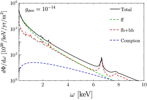
Figure 1: Scalar flux from the Sun. The coupling to electrons is chosen to be $g_{\phi ee}=10^{-14}$, and the scalar is taken to be massless. The green dashed line is Bremsstrahlung flux from electrons interacting with hydrogen and helium ions, the red dashed line is the flux due to recombination and transitions of bounded electrons in heavier elements, the blue dashed line is the flux from Compton-like scattering, and black line is the total scalar flux.

We finally comment on the resonant production of light scalars in the plasma. The scalar field with interaction Eq. (1) can mix with the longitudinal excitation of the photon in the plasma Hardy:2016kme (see also Refs. An:2013yfc ; Redondo:2013lna for earlier studies on the mixing of dark photon with the longitudinal photon mode in the Sun). In the presence of such mixing, the production rate of the scalar field changes as

$$\Gamma^{\textrm{prod}}\!\left(\omega\right)=\frac{g_{\phi ee}^{2}v_{\phi}^{2}}{4\pi\alpha_{\textrm{em}}}\frac{f\!\left(\omega\right)\Gamma_{L}\!\left(\omega\right)}{\left(1-\frac{\omega_{\textrm{p}}^{2}}{\omega^{2}}\right)^{2}+\left(\frac{\Gamma_{L}}{\omega}\right)^{2}}\,,$$ (12)

where $\omega_{\textrm{p}}^{2}=4\pi\alpha_{\textrm{em}}n_{e}/m_{e}$ is the plasma frequency, and $\Gamma_{L}=\Gamma_{L}^{\rm abs}-\Gamma_{L}^{\rm prod}$ is the damping rate of the longitudinal excitation of the photon. The term on the numerator is the production rate of the longitudinal mode, $\Gamma_{L}^{\rm prod}=f\!\left(\omega\right)\Gamma_{L}$, which can be seen by using detailed balance. The resonance takes place when the frequency of the scalar particle is close to the plasma frequency, $\omega\approx\omega_{\textrm{p}}$, and numerically, the flux at this frequency could be enhanced roughly by two or three orders of magnitude compared to the non-resonant case. However, the plasma frequency inside the Sun ranges as $1~{}\mathrm{eV}\lesssim\omega_{\textrm{p}}\lesssim 300~{}\mathrm{eV}$, and thus, the frequency of resonantly produced scalar particles is also limited from above by $300~{}\mathrm{eV}$. This energy scale is too small for the analysis of prompt scintillation signals, but is relevant for analysis of ionization signals in LXe detectors, as we will discuss below.

III Scalar absorption in detectors

Once the light states are produced in the Sun, they pass through the detectors, and are expected to ionize atoms due to the same interaction, Eq. (1). This effect is similar to the photoelectric effect. The expected event rate is obtained by the convolution of the solar flux, Eq. (3), with the absorption cross-section. Instead of directly computing the absorption cross-section, we use again the relation between matrix elements, Eq. (4), and estimate the absorption cross-section as a function of the photoelectric cross-section,

$$\frac{\sigma\!\left(\omega\right)v_{\phi}}{\sigma_{\textrm{pe}}\!\left(\omega\right)c}=\frac{g_{\phi ee}^{2}v_{\phi}^{2}}{4\pi\alpha_{\rm em}}\,,$$ (13)

where $\sigma_{\textrm{pe}}$ is the photoelectric cross-section for LXe. We ignore mixing of scalar particle with longitudinal excitation in the detector, since we are interested in scalar particles with $\omega\simeq{\cal O}\!\left(1\right)~{}\mathrm{keV}$, and for this frequency range, the mixing is barely important. For the photoelectric cross-section, we take tabulated data of $\sigma_{\rm pe}$ from Refs. Veigele:1973tza ; XCOM .

Having determined the flux and absorption cross-section, we use three sets of data, obtained by the XENON1T and LUX collaborations, to set limits on the coupling of scalar particles to electrons. We first discuss the prompt scintillation signals (denoted as S1). We use LUX data, collected in 2013 with an exposure of $95~{}\mathrm{days}$ and $118~{}\mathrm{kg}$ of fiducial mass, which is the same data set used by LUX collaboration to search for solar axions Akerib:2017uem . In addition, we use the XENON1T data set with an exposure of $1~{}\mathrm{ton\times yr}$, which has been used to probe weakly interacting massive particle (WIMP) DM Aprile:2018dbl .

The detector response is taken into account in the following way. First, the deposited energy is translated into expected S1 signal using ${\rm S1}=g_{1}\omega L_{y}$. The light yield, $L_{y}$, is the expected number of scintillation photons for a given energy deposition, and is taken from Ref. Akerib:2016qlr both for the LUX and XENON1T analyses. The detection efficiency for photons, $g_{1}$, is taken from Ref. Akerib:2017uem for the LUX analysis, and from Ref. Aprile:2019dme for the XENON1T analysis. Then, the observed S1 signal in the detector is obtained by Poisson-smearing and binning the expected signal.

For this analysis, we place a threshold of 3  photoelectrons (PE) in S1, and set $L_{y}$ to zero below the lowest measured data point of $1.3~{}\mathrm{keV}$. This procedure is established in order to avoid oversensitive response to the steeply raising solar flux below $1~{}\mathrm{keV}$, and can be relaxed in a future more elaborated analysis.

Several systematic studies have been performed to quantify the effect of below-threshold energy deposition. In particular, the light yield was extrapolated down to zero energy, the Poisson smearing was replaced by a Gaussian one, following the procedure described in Ref. Akerib:2016qlr , and the results were compared to no smearing with a hard cut at $1.5~{}\mathrm{keV}$ (which is equivalent to 3 PE). For all of these studies, the resulting limits have changed by less than 5%.

A profile likelihood procedure Cowan:2010js has been used to calculate the upper bounds on $g_{\phi ee}$ at 90% confidence level (CL). We use a binned likelihood function, which is a product of the Poisson probability of each bin (c.f. Ref. Patrignani:2016xqp ).

The expected number of signal events in each energy bin is estimated as described in the preceding section, and the expected number of background events in each bin is taken from Ref. Akerib:2017uem for LUX, and from Ref. Aprile:2018dbl for XENON1T. For LUX, we use 11 bins in the range of 3-60 PE, and for XENON1T we use a single bin in the range of 3-10 PE. As the XENON1T data is not binned, we estimate the background by assuming a flat background in S1 space. This assumption results in 66 expected background events in the search region. The number of data points in the search region was estimated to be 70.

We have also performed an S2-only analysis. The scalar flux produced in the Sun is enhanced at low energies by a resonant production, as mentioned above. Therefore, a search with lower threshold will yield much higher sensitivities, given that the background can be modeled, and that its rate is not exponentially raising. This technique has been used before in XENON100 Aprile:2016wwo , and recently in XENON1T Aprile:2019xxb , where the threshold was lowered by an order of magnitude with respect to S1-only analysis. We take the XENON1T data set Aprile:2019xxb with an exposure of $22~{}\mathrm{tonne\textrm{--}days}$ for the S2-only analysis, and use the detector response model presented in Ref. Aprile:2019dme to translate the deposited energy into S2 signals. As in Ref. Aprile:2019xxb , we assume that the electronic-recoil events below $186~{}\mathrm{eV}$ are undetectable for a conservative estimate. Then, we perform the same likelihood analysis to obtain an upper limit on $g_{\phi ee}$. The signal model, as well as data points and partial background model from XENON1T, are presented in Fig. 2.

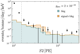
Figure 2: The black dots are the data with error bars showing statistical uncertainties ($1\sigma$ Poisson), the blue shaded histogram is the partial background model from XENON1T experiment, and the vertical dashed line shows the S2 threshold Aprile:2019xxb . The orange shaded histogram, stacked on the background, is the signal model for a massless scalar, and $g_{\phi ee}=2\times 10^{-15}$. There is a peak around S2 = 300–400 PE, which corresponds to the resonant peak of the scalar spectrum at $\omega\sim 0.2~{}\mathrm{keV}$.

IV Results and Discussions

We summarize our results for the S1-only analysis in Fig. 3. In the limit where the scalar mass can be ignored, the bound on $g_{\phi ee}$ becomes

$$g_{\phi ee} <2\times 10^{-14}\qquad\textrm{(\acs{LUX})}$$ (14)

$$g_{\phi ee} <7\times 10^{-15}\qquad\textrm{(XENON1T)}$$ (15)

at 90% CL. In addition to these experiments, we also show the projected sensitivity of XENONnT. Since the total event rate at the detector is proportional to $g_{\phi ee}^{4}$, the expected improvement on the electron coupling only scales as a fourth root of the exposure. The projected limit of XENONnT with a total exposure of $20~{}\mathrm{ton\times yr}$, and an assumed flat background rate of $1000~{}\mathrm{events/ton/year}$ Aprile:2015uzo yields

$$\ g_{\phi ee}<3\times 10^{-15}\qquad\textrm{(XENONnT, projected)}\,.$$ (16)

Again, this bound is valid for $m_{\phi}<1~{}\mathrm{keV}$. In the same figure, we also present the constraints from the other searches on $g_{\phi ee}$. As we consider new light particles below keV, the most stringent constraints come from astrophysical observations. Since the electron coupling to a light scalar state opens additional channels for these astrophysical objects to lose their energy, it can lead to anomalous cooling of stellar objects, such as red giants, and stars on the horizontal branch. Non-observation of such anomalous cooling of stellar objects could place a constraint on a possible electron coupling to any new light states Raffelt:1996wa . Compared to the results of earlier studies on scalar-electron coupling, $g_{\phi ee}<11\times 10^{-15}$ Grifols:1988fv ; Raffelt:1996wa , our result is a factor few better. However, a recent study has improved the stellar cooling bound on the same coupling to $g_{\phi ee}<7\times 10^{-16}$, when accounting for in-medium mixing effect of the scalar field Hardy:2016kme . Compared to the latest stellar cooling bound, our current S1-only limit, obtained from XENON1T data, is about an order of magnitude weaker.

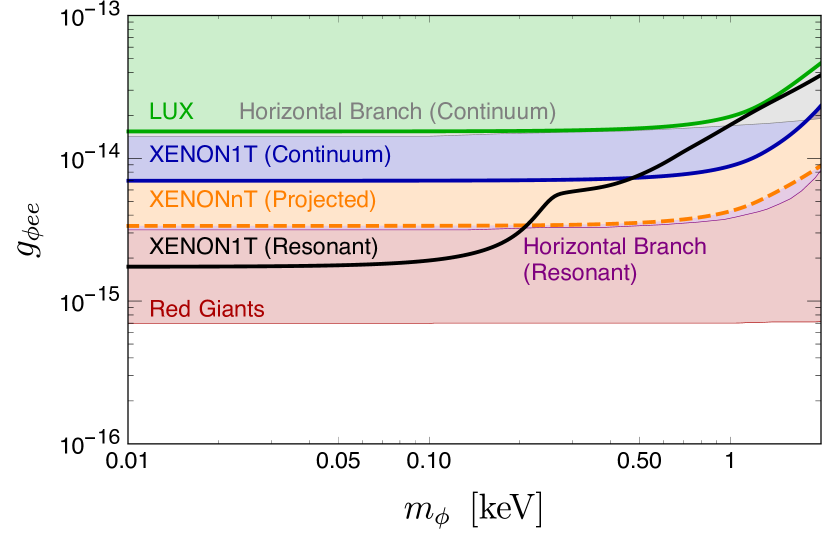
Figure 3: Constraints on the coupling $g_{\phi ee}$. The result of this work includes the green thick solid line (LUX), the blue thick solid line (XENON1T), the orange thick dashed line (projected sensitivity of XENONnT experiment with $20~{}\mathrm{ton\times yr}$ exposure), and the black thick solid line (XENON1T S2-only analysis, capturing the resonant production). The thin red, purple, and gray lines represent stellar cooling bounds from red giants, horizontal branch stars with and without in-medium mixing effect Hardy:2016kme , respectively.

We also present the result of S2-only analysis. From the recent data of XENON1T experiment Aprile:2019xxb , we find

$$g_{\phi ee}<2\times 10^{-15}$$ (17)

at 90% CL. This bound is valid for $m_{\phi}\lesssim 0.1~{}\mathrm{keV}$, since the constraining power mainly comes from a resonant peak in the signal. The sensitivity of the XENON1T S2-only analysis is a factor three weaker than the strongest stellar cooling bound. Upper limits on $g_{\phi ee}$ for scalar masses larger than $0.01~{}\mathrm{keV}$ are presented in Fig. 3

Our result can be interpreted in the context of several theoretically well-motivated new physics scenarios. Examples include a cosmological relaxion, and Higgs portal singlet scalar field. In both scenarios, a scalar state naturally mixes with the SM Higgs boson, and thus becomes coupled to the SM particles with coupling constant given by

$$g_{\phi\psi\psi}=g_{\psi}\sin\theta\,,$$ (18)

where $g_{\psi}$ is the standard Higgs coupling to SM fermions, and $\sin\theta$ is the scalar-Higgs mixing angle. For electron coupling, $g_{e}=\kappa_{e}m_{e}/\upsilon=3\times 10^{-6}\left(\kappa_{e}/1\right)$, where $\upsilon=174~{}\mathrm{GeV}$ is the electroweak scale, and in the SM, $\kappa_{e}=1$. Direct searches for Higgs decay and resonant production allow for a $600$ times stronger interaction strength with electrons than the predicted SM value Altmannshofer:2015qra , i.e. $\kappa_{e}=600$. Our bound, Eq. (17), can be thus interpreted as a bound on the mixing angle

$$\sin\theta<\begin{cases}7\times 10^{-10}&\kappa_{e}=1\\ 1\times 10^{-12}&\kappa_{e}=600\end{cases}\,.$$ (19)

This applies to any scalar that mixes with the Higgs. For Higgs portal models (see e.g. Ref. Piazza:2010ye ), the scalar mass receives a radiative correction from its mixing with Higgs, $\Delta m_{\phi}^{2}\simeq\upsilon^{2}\sin^{2}\theta/16\pi^{2}$, and thus, a natural model requires

$$\sin\theta\lesssim\frac{4\pi m_{\phi}}{\upsilon}=7\times 10^{-9}\cdot\left(\frac{m_{\phi}}{100~{}\mathrm{eV}}\right)\,,$$ (20)

hence our bound probes natural models. For a generic scalar particle which couples to the electron, the scalar mass receives a quadratically divergent radiative correction from an electron loop, and the cutoff of the theory is bounded by the same naturalness argument as

$$\Lambda_{\textrm{NP}} \lesssim\frac{4\pi m_{\phi}}{g_{\phi ee}}\lesssim 6\times 10^{5}~{}\mathrm{TeV}\cdot\left(\frac{m_{\phi}}{100~{}\mathrm{eV}}\right)\,.$$ (21)

In this paper, we have considered solar production of light scalar particles, and used LXe detectors, XENON1T and LUX, to probe its coupling to electrons. We have only considered a subset of DM direct detectors, which has been mainly focusing on detection of WIMP DM. Another interesting direction is to use newly proposed ideas on DM direct detection, making use of inter-atomic interactions to lower the threshold (see e.g. Refs. Battaglieri:2017aum ; Lin:2019uvt and references therein). Such experiments provide an alternative probe of scalar-electron coupling, as the flux of scalar field from the Sun could be resonantly enhanced.

V Acknowledgments

The work of RB is supported by grants from ISF (1295/18), and Pazy-VATAT. RB is the incumbent of the Arye and Ido Dissentshik Career Development Chair. The work of GP is supported by grants from the BSF, ERC, ISF, Minerva Foundation, and the Segre Research Award. NP is partially supported by the Koret Foundation.

SM

Standard Model

ALP

axion-like particle

WIMP

weakly interacting massive particle

DM

dark matter

LXe

liquid xenon

LUX

Large Underground Xenon

PE

photoelectrons

CL

confidence level

References

- (1) P. W. Graham, D. E. Kaplan, and S. Rajendran, Phys. Rev. Lett. 115, 221801 (2015), arXiv:1504.07551.
- (2) T. Flacke, C. Frugiuele, E. Fuchs, R. S. Gupta, and G. Perez, JHEP 06, 050 (2017), arXiv:1610.02025.
- (3) K. Choi and S. H. Im, JHEP 12, 093 (2016), arXiv:1610.00680.
- (4) J. Beacham et al., (2019), arXiv:1901.09966.
- (5) G. Krnjaic, Phys. Rev. D94, 073009 (2016), arXiv:1512.04119.
- (6) C. Frugiuele, E. Fuchs, G. Perez, and M. Schlaffer, JHEP 10, 151 (2018), arXiv:1807.10842.
- (7) A. Fradette, M. Pospelov, J. Pradler, and A. Ritz, Phys. Rev. D99, 075004 (2019), arXiv:1812.07585.
- (8) A. Arvanitaki, J. Huang, and K. Van Tilburg, Phys. Rev. D91, 015015 (2015), arXiv:1405.2925.
- (9) P. W. Graham, D. E. Kaplan, J. Mardon, S. Rajendran, and W. A. Terrano, Phys. Rev. D93, 075029 (2016), arXiv:1512.06165.
- (10) A. Arvanitaki, S. Dimopoulos, and K. Van Tilburg, Phys. Rev. X8, 041001 (2018), arXiv:1709.05354.
- (11) M. S. Safronova et al., Rev. Mod. Phys. 90, 025008 (2018), arXiv:1710.01833.
- (12) A. Banerjee, H. Kim, and G. Perez, (2018), arXiv:1810.01889.
- (13) S. Aharony et al., (2019), arXiv:1902.02788.
- (14) D. Antypas et al., (2019), arXiv:1905.02968.
- (15) S. Dimopoulos, G. D. Starkman, and B. W. Lynn, Phys. Lett. 168B, 145 (1986).
- (16) F. T. Avignone, III et al., Phys. Rev. D35, 2752 (1987).
- (17) E. Armengaud et al., JCAP 1311, 067 (2013), arXiv:1307.1488.
- (18) XENON100, E. Aprile et al., Phys. Rev. D90, 062009 (2014), arXiv:1404.1455, [Erratum: Phys. Rev.D95,no.2,029904(2017)].
- (19) LUX, D. S. Akerib et al., Phys. Rev. Lett. 118, 261301 (2017), arXiv:1704.02297.
- (20) CDMS, Z. Ahmed et al., Phys. Rev. Lett. 103, 141802 (2009), arXiv:0902.4693.
- (21) KIMS, Y. S. Yoon et al., JHEP 06, 011 (2016), arXiv:1604.01825.
- (22) K. Abe et al., Phys. Lett. B724, 46 (2013), arXiv:1212.6153.
- (23) H. An, M. Pospelov, and J. Pradler, Phys. Rev. Lett. 111, 041302 (2013), arXiv:1304.3461.
- (24) I. M. Bloch, R. Essig, K. Tobioka, T. Volansky, and T.-T. Yu, JHEP 06, 087 (2017), arXiv:1608.02123.
- (25) Y. Hochberg, T. Lin, and K. M. Zurek, Phys. Rev. D95, 023013 (2017), arXiv:1608.01994.
- (26) J. Redondo and G. Raffelt, JCAP 1308, 034 (2013), arXiv:1305.2920.
- (27) N. R. Badnell et al., Mon. Not. Roy. Astron. Soc. 360, 458 (2005), arXiv:astro-ph/0410744.
- (28) M. J. Seaton, Mon. Not. Roy. Astron. Soc. 362, 1 (2005), arXiv:astro-ph/0411010.
- (29) http://cdsweb.u-strasbg.fr/topbase/TheOP.html.
- (30) J. Redondo, JCAP 1312, 008 (2013), arXiv:1310.0823.
- (31) N. Vinyoles et al., Astrophys. J. 835, 202 (2017), arXiv:1611.09867.
- (32) E. Hardy and R. Lasenby, JHEP 02, 033 (2017), arXiv:1611.05852.
- (33) H. An, M. Pospelov, and J. Pradler, Phys. Lett. B725, 190 (2013), arXiv:1302.3884.
- (34) W. J. Veigele, Atom. Data Nucl. Data Tabl. 5, 51 (1973).
- (35) M. J. Berger et al., Xcom: Photon cross sections databas., Online, 2010.
- (36) XENON, E. Aprile et al., Phys. Rev. Lett. 121, 111302 (2018), arXiv:1805.12562.
- (37) LUX, D. S. Akerib et al., Phys. Rev. D95, 012008 (2017), arXiv:1610.02076.
- (38) XENON, E. Aprile et al., Phys. Rev. D99, 112009 (2019), arXiv:1902.11297.
- (39) G. Cowan, K. Cranmer, E. Gross, and O. Vitells, Eur. Phys. J. C71, 1554 (2011), arXiv:1007.1727, [Erratum: Eur. Phys. J.C73,2501(2013)].
- (40) Particle Data Group, C. Patrignani et al., Chin. Phys. C40, 100001 (2016).
- (41) XENON, E. Aprile et al., Phys. Rev. D94, 092001 (2016), arXiv:1605.06262, [Erratum: Phys. Rev.D95,no.5,059901(2017)].
- (42) XENON, E. Aprile et al., (2019), arXiv:1907.11485.
- (43) XENON, E. Aprile et al., JCAP 1604, 027 (2016), arXiv:1512.07501.
- (44) G. G. Raffelt, Stars as laboratories for fundamental physics (, 1996).
- (45) J. A. Grifols, E. Masso, and S. Peris, Mod. Phys. Lett. A4, 311 (1989).
- (46) W. Altmannshofer, J. Brod, and M. Schmaltz, JHEP 05, 125 (2015), arXiv:1503.04830.
- (47) F. Piazza and M. Pospelov, Phys. Rev. D82, 043533 (2010), arXiv:1003.2313.
- (48) M. Battaglieri et al., US Cosmic Visions: New Ideas in Dark Matter 2017: Community Report, in U.S. Cosmic Visions: New Ideas in Dark Matter College Park, MD, USA, March 23-25, 2017, 2017, arXiv:1707.04591.
- (49) T. Lin, (2019), arXiv:1904.07915.