Elastic_HH: Tailored Elastic for
Finding Heavy Hitters

Abstract

Finding heavy hitters has been of vital importance in network measurement. Among all the recent works in finding heavy hitters, the Elastic sketch achieves the highest accuracy and fastest speed. However, we find that there is still room for improvement of the Elastic sketch in finding heavy hitters. In this paper, we propose a tailored Elastic to enhance the sketch only for finding heavy hitters at the cost of losing the generality of Elastic. To tailor Elastic, we abandon the light part, and improve the eviction strategy. Our experimental results show that compared with the standard Elastic, our tailored Elastic reduces the error rate to 5.7$\sim$8.1 times and increases the speed to 2.5 times. All the related source codes and datasets are available at Github [1].

I Introduction

I-A Motivation

Network measurement has been an important issue in networking. One kind of solution relying on sketches has attracted extensive attention in recent years [14, 23, 20, 24, 19, 16, 10, 8, 9, 17, 15]. In practice, the most important task is finding heavy hitters, i.e., finding flows with flow size larger than a threshold. Flow size is defined as the number of packets in a flow in this paper. Flow ID is often a combination of the five-tuples: source IP address, source port, destination IP address, destination port, protocol. Therefore, we survey various sketches proposed in recent years, and find that the Elastic sketch [23] exerts the highest accuracy and the fastest speed in finding heavy hitters.

The Elastic sketch [23] , the state-of-the-art, has a special property – generality. It can use one data structure to process six measurement tasks: flow size estimation, heavy hitter detection, heavy change detection, flow size distribution estimation, entropy estimation, and cardinality estimation. For finding heavy hitters, Elastic can achieve much higher accuracy and speed than other sketches, including Space-Saving [21], a sketch plus min-heap [7, 11, 6], CSS[4], HashPipe [22], and so on.

For the sake of generality, Elastic needs to record all necessary information. We argue that sacrificing the property of generality can potentially improve the accuracy and speed. In practice, some practical scenarios only need to find heavy hitters. When we manage to enhance Elastic for the single task – finding heavy hitters, we find that there is still room for improvement.

Therefore, the goal of this paper is to improve the accuracy and speed of Elastic for finding heavy hitters, at the cost of not supporting other tasks. This work is non-trivial, for finding heavy hitter is the most important task in network measurements[25, 5, 12] and it is often important to make in-time improvement for the state-of-the-art.

I-B Our Solution

In this paper, we propose a modification and an improvement to enhance the accuracy of Elastic. The data structure of Elastic has two parts: a heavy part recording elephant flows (large flows) and a light part recording mice flows (small flows). Our modification is to abandon the light part, for we only care about elephant flows, i.e., heavy hitters. This modification is simple but effective.

Our key improvement is to change the replacement strategy when evicting flows in the heavy part. We use a simple example to show how we improve the Elastic sketch. Suppose we want to use $k$ buckets to record the top-$k$ largest flows of a given network stream. The stream recording is considered as a voting process. Suppose that the smallest flow in the $k$ buckets is $f_{min}$ with size of $vote_{min}^{+}$. Given an incoming packet with flow ID $f_{1}$, it is a positive vote if $f_{1}$ exists in one of the $k$ buckets, otherwise, it is a negative vote. In the Elastic sketch, when $\frac{vote^{-}}{vote_{min}^{+}}\geqslant\lambda$ where $vote^{-}$ is the number of negative votes, $f_{min}$ in the bucket is replaced by $f_{1}$, and the size of the new inserted flow is set to 1. The authors of Elastic recommend setting $\lambda=8$. In our improvement, the replacement is activated when $vote^{-}\geqslant vote_{min}^{+}+1$, and the size of the new inserted flow is set to $f_{min}+1$ rather than 1. We argue that when the smallest flow is evicted by a new flow, the size of the new flow is probably larger than the smallest flow.

The modification and the improvement significantly enhance the accuracy of Elastic when finding heavy hitters. Our cost is that the generality of Elastic is lost. Therefore, when the applications only need to find heavy hitters, we recommend using our tailored Elastic sketch.

II Background and Related Work

In this section, we first show the details of the Elastic sketch, and then briefly survey the related work.

II-A The Elastic Sketch

Among all the versions of Elastic, the software version achieves the highest accuracy, therefore, we only show how the software version of Elastic works.

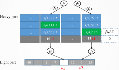
Figure 1: An example for the Elastic sketch.

Data Structure (Fig. 1): The data structure of the Elastic sketch consists of two parts. The first part is the heavy part consisting of many buckets. The number of buckets is determined by the available memory size and required accuracy bound. The detailed analysis can be seen in[23]. In each bucket, there are several cells, each of which stores three fields of a flow: flow ID (ID), positive votes ($vote^{+}$), and flag. The flag in each cell indicates whether there are evictions in the cell. There is an additional cell in each bucket recording the negative votes ($vote^{-}$). The second part is the light part storing the flow sizes of small flows.

Insertion (Fig. 1): For convenience, we use two examples to show the insertion operation of Elastic. Given an incoming packet with flow ID $f_{8}$, we calculate the hash function $h(f_{8})$ and find the hashed bucket. Since flow $f_{8}$ is not stored in the hashed bucket, $vote^{-}(=10)$ is incremented by one. After increment, we pick out the flow with the smallest size in the bucket, $f_{6}$, and calculate the value $\frac{vote^{-}}{vote^{+}}$, where $vote^{+}$ is the flow size of $f_{6}$. Since $\frac{vote^{-}}{vote^{+}}=\frac{11}{11}<\lambda(=8)$, $f_{8}$ is inserted into the light part and the corresponding counter is incremented by one. Given another incoming packet with flow ID $f_{9}$, we also calculate the hash function and read the hashed bucket. We find that $f_{9}$ is not stored in the bucket, so $vote^{-}(=55)$ is incremented by one. After finding the flow with the smallest size, $f_{4}$, we calculate the value of $\frac{vote^{-}}{vote^{+}}(=\frac{56}{7})$, which equals to $\lambda(=8)$. Therefore, $f_{4}$ is replaced by $f_{9}$ and the initial size of $f_{9}$ is set to 1. $vote^{-}$ is set to zero. Flow $f_{4}$ is evicted into the light part, and the corresponding counter of $f_{4}$ is incremented by 7, where 7 is the $vote^{+}$ of $f_{4}$ in the heavy part.

II-B Other Sketches for Heavy Hitters

There are many sketches for finding heavy hitters. Due to space limitation, this subsection only lists the typical sketches. There are two kinds of sketches. The first kind uses a sketch (such as sketches of CM[7], CU [11], Count [6], CSM [18]) plus a min-heap. Among them, the CU sketch achieves the highest accuracy and the CSM sketch achieves the fastest speed. The second kind is Space-Saving [21] and its variants. Typical variants include CSS [4], FSS[13], Hash-Pipe [22], and PRECISION [3].

III The Elastic_HH Sketch

In this section, we tailor the Elastic sketch for finding heavy hitters, namely Elastic_HH for convenience. We present the details of Elastic_HH, including data structure, insertion, report, and analysis.

III-A Data Structure

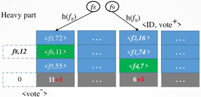
Figure 2: An example for the Elastic_HH.

Data Structure (Fig. 1): The data structure of Elastic_HH only keeps the heavy part which consists of many buckets. The number of buckets is determined by the available memory size and required accuracy bound. In each bucket, there are several cells: one cell records the negative votes ($vote^{-}$) of the bucket, and the other cells store two fields of a flow: flow ID (ID) and positive votes ($vote^{+}$, i.e., flow size).

III-B Operations

Insertion (Fig. 2): When inserting an incoming packet with flow ID $f$, we first calculate the hash function and check the hashed bucket:

1) If $f$ is in the bucket, we only increment the corresponding positive votes ($vote^{+}$);

2) If $f$ is not in the bucket, there are the following two cases:

Case 1: There are empty cells in the bucket. We just insert $f$ with $vote^{+}$ of 1 into the first empty cell;

Case 2: There is no empty cell in the bucket. We first increment $vote^{-}$ by 1. Then we compare $vote^{-}$with the smallest positive votes $vote^{+}_{min}$ in the bucket. If $vote^{-}>vote^{+}_{min}(\lambda=1)$, the smallest flow is replaced by $f$ and $vote^{+}_{min}$ is incremented by 1; Otherwise, $f$ is discarded.

Examples (Fig. 2): We use two examples to show the differences between the standard Elastic and our tailored Elastic in terms of the insertion operation. Given an incoming packet with flow ID $f_{8}$, the hash function $h(f_{8})$ is calculated and the hashed bucket is found. Since flow $f_{8}$ is not stored in the bucket, $vote^{-}(=11)$ is incremented by 1. We find flow $f_{6}$, the flow with the smallest size in the bucket. Because $vote^{-}(=12)$ is larger than ${vote^{+}(=11)}$ of $f_{6}$, $f_{6}$ is replaced by $f_{8}$, and the size of $f_{8}$ is set to $vote^{-}$ (12, i.e., $vote^{+}$ of $f_{6}$ plus 1). Flow $f_{6}$ is discarded and $vote^{-}$ is set to zero. For another incoming packet with flow ID $f_{9}$, we calculate the hash function and find the hashed bucket. Since $f_{9}$ is not stored in the bucket, $vote^{-}(=6)$ is incremented by one. We then find the flow with the smallest size, $f_{4}$, and find that $vote^{-}$ is not larger than ${vote^{+}(=7)}$ of $f_{4}$. Therefore, $f_{9}$ is discarded and nothing else is changed.

Report (Fig. 2): To report heavy hitters, we simply traverse all cells in every bucket, and report all flows with flow size larger than a threshold.

III-C Analysis

We analyze our method from the following aspects.

First, the light part of the Elastic for small flows is abandoned and thus memory is saved. Without the light part, to keep most heavy hitters in the heavy part, the adjustment of value of $\lambda$, which decides the number of evictions, becomes important. As the value of $\lambda$ increases, the number of evictions decreases. To make heavy hitters into the heavy part more easily and achieve higher accuracy, choosing a small $\lambda$ is better. According to our experimental results on different datasets, we find when $\lambda=1$, the accuracy is nearly optimal and there is no computation cost for $*1$. Therefore, we adjust $\lambda=1$ in the Elastic_HH but not $\lambda=8$ in the original Elastic sketch.

Second, for any incoming random flow f, it must be either a large flow or a small flow, like with size of 1. We do not know its size before-hand and the Elastic_HH will treat flows differently according to its size. For the incoming large flows, there are two common cases. The first case is when there is an empty cell in the hashed bucket. We just insert the flow into the cell. Since it is a large flow, it is often not the smallest one in the bucket, and thus it is safe from being evicted/replaced. The second case is when there is no empty cell in the hashed bucket. The large flow will use $vote^{+}_{min}+1$ packets to evict the smallest flow, and then be inserted into the bucket. For these two cases, the error is very small. For a flow with size of 1, it might be lucky to be kept and become the smallest flow with size $vote^{+}_{min}$ in the hashed bucket. However, it will be replaced after $vote^{+}_{min}+1$ packets of other flows arrive.

Third, for each insertion, we at most access all cells in one bucket, and reading continuous cells is very fast because of good cache behaviour.

IV Experimental Results

In this section, we provide experimental results of Elastic_HH compared with state-of-the-art algorithms in finding heavy hitters. After introducing the Experimental Setup in Section IV-A, we evaluate different algorithms on accuracy and processing speed in Section IV-B.

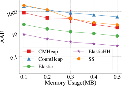
(a) AAE

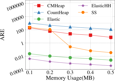
(b) ARE

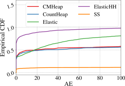
(c) Empirical CDF of AE

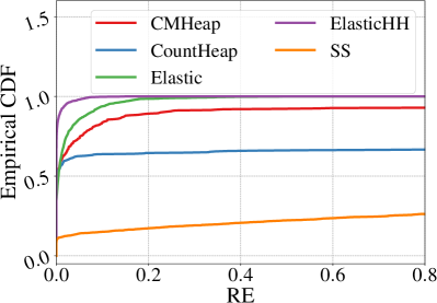
(d) Empirical CDF of RE

Figure 3: Accuracy comparison for heavy hitter detection

IV-A Experimental Setup

IP Trace Dataset: We use the public traffic trace datasets collected in Equinix-Chicago monitor from CAIDA[2]. In our experiments, each packet is identified by its source IP address (4 bytes).

Implementation: For finding heavy hitters (HH), we compare five approaches: Space-Saving (SS)[21], Count/CM Sketch[7, 6] with a min-heap (CountHeap/CMHeap), Elastic (the software version)[23], and Elastic_HH, all of which are implemented in C++. For the above five algorithms, the default memory size is 300KB and we set the heavy hitter threshold to 0.01% of the number of all packets in every experiment. For both Elastic and Elastic_HH, we use the parameters in the open-sourced code of Elastic. Specifically, we store 7 flows and one $vote^{-}$ in each bucket of the heavy part. The ratio of the heavy part and the light part is set to 3:1 for Elastic. For CountHeap/CMHeap, we use 3 hash functions for the sketch and set the heap capacity to 4096 nodes.

Computation Platform: we conducted all the experiments on a machine with one 4-core processor (8 threads, Intel Core i7-8550U@1.80GHz) and 15.4 GB DRAM memory. To accelerate the processing speed, we use SIMD (Single Instruction Multiple Data) instructions for both Elastic and Elastic_HH. With the AVX2 instruction set, we can find the minimum counter and its index among 8 counters in a single comparison instruction. Also, we can compare 8 32-bit integers with another set of 8 32-bit integers in a single instruction.

Metrics: We use the following eight metrics to evaluate the performance of compared algorithms.

1) AAE (Average Absolute Error): $\frac{1}{|\mathchar 264\relax|}\sum_{e_{i}\in\mathchar 264\relax}|f_{i}-\hat{f_{i}}|$, where $\mathchar 264\relax$ is the query set of flows and $f_{i}$ and $\hat{f_{i}}$ are the actual and estimated flow sizes of flow $f_{i}$, respectively. Note that we use $f_{i}$ to denote both the $i^{th}$ flow and its size.

2) ARE (Average Relative Error): $\frac{1}{|\mathchar 264\relax|}\sum_{e_{i}\in\mathchar 264\relax}\frac{|f_{i}-\hat{f_{i}}|}{f_{i}}$, where $\mathchar 264\relax$, $f_{i}$, and $\hat{f_{i}}$ are defined above.

3) PR (Precision Rate): Ratio of the number of correctly reported flows to the number of reported flows.

4) RR (Recall Rate): Ratio of the number of correctly reported flows to the number of true flows.

5) $\mathbf{F_{1}}$ score: $\frac{2\times PR\times RR}{PR+RR}$, where PR and RR are defined above.

6) AE (Absolute Error): $|True-Estimated|$, where $True$ and $Estimated$ represent the actual and estimated size of a flow. We use its Cumulative Distribution Function (CDF) to evaluate the AE’s distribution of different algorithms.

7) RE (Relative Error): $|\frac{True-Estimated}{True}|$, where $True$ and $Estimated$ have the same definitions as above. We also evaluate the CDF of RE.

8) Throughput: million packets per second (Mpps). We use it to evaluate the processing speed of different sketches. The experiments on processing speed are repeated 100 times to minimize accidental errors.

IV-B Evaluation on Accuracy and Processing Speed

AAE and ARE (Figure 3(a)-3(b)): Our experimental results show that Elastic_HH achieves the highest accuracy, followed by Elastic. Compared with Elastic, Elastic_HH achieves $7.3\sim 8.1$ times smaller AAE and $5.7\sim 7.5$ times smaller ARE. In this experiment, we set the size of memory between 100KB and 500KB.

Empirical CDF of AE (Figure 3(c)): Our experimental results show that when memory size is set to 100KB, for Elastic_HH, more than 90% reported heavy hitters have an AE less than 24; while for Elastic, the number is only 56%. As for the other three algorithms, CMHeap and CountHeap have 49% and 51% reported heavy hitters whose AEs are less than 24; while for SS, the number is only 11%. Note that, as AE increases, for Elastic_HH, the empirical CDF increases significantly; while for Elastic, CMHeap and CountHeap, the empirical CDF increases slowly; and for SS, the empirical CDF keeps at a low value. This result indicates that, the estimated frequencies of most flows of Elastic_HH are accurate; while for other algorithms, their flows suffer from large errors.

Empirical CDF of RE (Figure 3(d)): Our experimental results show that when memory size is set to 100KB, for Elastic_HH, more than 90% reported heavy hitters have an RE less than 0.008; while for Elastic and CMHeap, the corresponding REs are 0.075 and 0.233, respectively. For CountHeap and SS, their corresponding RE are more than 500. Note that, as RE increases, the empirical CDF of Elastic_HH, Elastic and CMHeap all increase significantly and the empirical CDF of Elastic_HH increases the fastest. This result is consistent with the result we analyzed in the evaluation of the empirical CDF of AE.

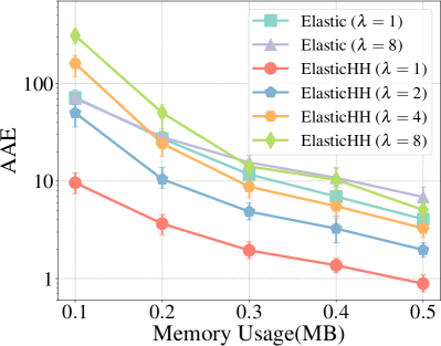
(a) AAE

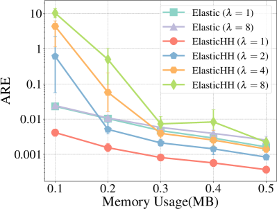
(b) ARE

Figure 4: Accuracy comparison for value of different $\lambda$ in Elastic and Elastic_HH

AAE and ARE comparison of Elastic_HH with different $\lambda$ (Figure 4(a)-4(b)): Our experimental results show that Elastic_HH with $\lambda=1$ achieves the highest accuracy. As $\lambda$ gets smaller, the accuracy is much higher for Elastic_HH. The accuracy of Elastic with $\lambda=8$ is better than Elastic_HH. However, it doesn’t improve its accuracy when $\lambda=1$ and thus is worse than Elastic_HH when $\lambda=1$. Compared with Elastic, Elastic_HH achieves $4.4\sim 8.2$ times smaller AAE and $4.4\sim 6.9$ times smaller ARE when $\lambda=1$. In this experiment, we set the size of memory between 100KB and 500KB.

PR, RR and $\mathbf{F_{1}}$ score (Figure 5(a)-5(c)): Our experimental results show that for our Elastic_HH, PR, RR and $F_{1}$ score all achieve nearly 100% even when memory size is set to 100KB; while for Elastic, its RR and $F_{1}$ score get lower when memory size is set to 100KB.

For the other three algorithms, their PR, RR and $F_{1}$ score can only increase to nearly 100% when memory size is set to at least 400KB, or even larger.

Throughput (Figure 5(d)): Our experimental results show that on our tested CPU platform, Elastic_HH achieves much higher throughput than other four algorithms. Compared to Elastic, Elastic_HH is about 2.5 times faster. Other three conventional algorithms can only reach a throughput no faster than 15Mpps (million packets per second), while Elastic_HH can reach more than 160Mpps after using SIMD.

Summary: 1) For the same memory size and the same dataset, the accuracy of our Elastic_HH is much better in terms of all metrics: AAE, ARE, Empirical CDF of AE and RE. As for PR, RR and $F_{1}$ score, our Elastic_HH has reached nearly 100% accuracy. 2) For the same memory size and the same dataset, the accuracy of our Elastic_HH with $\lambda=1$ is better than with other $\lambda$ values larger than 1 in terms of metrics: AAE and ARE. As $*1$ doesn’t require additional computations, its processing speed is faster than with other $\lambda$ values, including the ones smaller than 1. 3) For the same memory size and the same dataset, the processing speed of our Elastic_HH is 2.5 times faster than Elastic. As our Elastic_HH uses SIMD instructions, it can reach more than 10 times faster processing speed than other three algorithms, respectively.

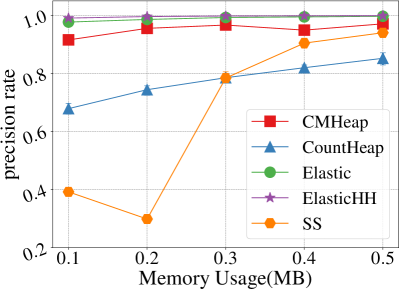
(a) precision rate

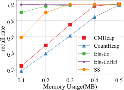
(b) recall rate

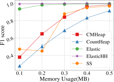
(c) F1 socre

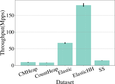
(d) Throughput

Figure 5: Processing speed and accuracy comparison for heavy hitter detection

V Conclusion

For finding heavy hitters, the Elastic sketch achieves the highest accuracy. However, we find that the accuracy of the Elastic sketch can be improved. In this paper, we propose a tailored Elastic to enhance the sketch only for finding heavy hitters by sacrificing the generality of Elastic. Our key improvement is when the number of negative votes is larger than that of the smallest positive votes, we evict the smallest flow and set the flow size of the new flow to the smallest positive votes plus 1 ($\lambda=1$). Experimental results show that using our improvement, the error rate is reduced to $5.7\sim 8.1$ times, and the speed is increased to about 2.5 times.

References

- [1] The source codes of our and other related algorithms. https://github.com/ElasticHH/Elastic_HH.
- [2] The CAIDA Anonymized Internet Traces. http://www.caida.org/data/overview/.
- [3] R. B. Basat, X. Chen, G. Einziger, and O. Rottenstreich. Efficient measurement on programmable switches using probabilistic recirculation. In Proc. IEEE ICNP, 2018.
- [4] R. Ben-Basat, G. Einziger, R. Friedman, and Y. Kassner. Heavy hitters in streams and sliding windows. In Proc. IEEE INFOCOM, 2016.
- [5] R. Ben Basat, G. Einziger, R. Friedman, M. C. Luizelli, and E. Waisbard. Constant time updates in hierarchical heavy hitters. In Proceedings of the Conference of the ACM Special Interest Group on Data Communication, pages 127–140. ACM, 2017.
- [6] M. Charikar, K. Chen, and M. Farach-Colton. Finding frequent items in data streams. Automata, languages and programming, 2002.
- [7] G. Cormode and S. Muthukrishnan. An improved data stream summary: the count-min sketch and its applications. Journal of Algorithms, 55(1), 2005.
- [8] H. Dai, L. Meng, and A. X. Liu. Finding persistent items in distributed, datasets. In Proc. IEEE INFOCOM, 2018.
- [9] H. Dai, M. Shahzad, A. X. Liu, and Y. Zhong. Finding persistent items in data streams. Proceedings of the VLDB Endowment, 10(4):289–300, 2016.
- [10] H. Dai, Y. Zhong, A. X. Liu, W. Wang, and M. Li. Noisy bloom filters for multi-set membership testing. In Proc. ACM SIGMETRICS, pages 139–151, 2016.
- [11] C. Estan and G. Varghese. New directions in traffic measurement and accounting: Focusing on the elephants, ignoring the mice. ACM Transactions on Computer Systems (TOCS), 21(3), 2003.
- [12] R. Harrison, Q. Cai, A. Gupta, and J. Rexford. Network-wide heavy hitter detection with commodity switches. In Proceedings of the Symposium on SDN Research, page 8. ACM, 2018.
- [13] N. Homem and J. P. Carvalho. Finding top-k elements in data streams. Information Sciences, 180(24):4958–4974, 2010.
- [14] Q. Huang, X. Jin, P. P. Lee, R. Li, L. Tang, Y.-C. Chen, and G. Zhang. Sketchvisor: Robust network measurement for software packet processing. In Proceedings of the Conference of the ACM Special Interest Group on Data Communication. ACM, 2017.
- [15] Q. Huang and P. P. Lee. Ld-sketch: A distributed sketching design for accurate and scalable anomaly detection in network data streams. In IEEE INFOCOM 2014-IEEE Conference on Computer Communications, pages 1420–1428. IEEE, 2014.
- [16] Q. Huang, P. P. Lee, and Y. Bao. Sketchlearn: relieving user burdens in approximate measurement with automated statistical inference. In Proceedings of the 2018 Conference of the ACM Special Interest Group on Data Communication, pages 576–590. ACM, 2018.
- [17] D. Li, H. Cui, Y. Hu, Y. Xia, and X. Wang. Scalable data center multicast using multi-class bloom filter. In 2011 19th IEEE International Conference on Network Protocols, pages 266–275. IEEE, 2011.
- [18] T. Li, S. Chen, and Y. Ling. Per-flow traffic measurement through randomized counter sharing. IEEE/ACM Transactions on Networking (TON), 20(5), 2012.
- [19] Y. Li, R. Miao, C. Kim, and M. Yu. Flowradar: A better netflow for data centers. In NSDI, 2016.
- [20] Z. Liu, A. Manousis, G. Vorsanger, V. Sekar, and V. Braverman. One sketch to rule them all: Rethinking network flow monitoring with univmon. In Proceedings of the 2016 conference on ACM SIGCOMM 2016 Conference. ACM, 2016.
- [21] A. Metwally, D. Agrawal, and A. El Abbadi. Efficient computation of frequent and top-k elements in data streams. In Proc. Springer ICDT, 2005.
- [22] V. Sivaraman, S. Narayana, O. Rottenstreich, S. Muthukrishnan, and J. Rexford. Heavy-hitter detection entirely in the data plane. In Proceedings of the Symposium on SDN Research. ACM, 2017.
- [23] T. Yang, J. Jiang, P. Liu, Q. Huang, J. Gong, Y. Zhou, R. Miao, X. Li, and S. Uhlig. Elastic sketch: Adaptive and fast network-wide measurements. In Proceedings of the 2018 ACM SIGCOMM Conference. ACM, 2018.
- [24] M. Yu, L. Jose, and R. Miao. Software defined traffic measurement with opensketch. In NSDI, volume 13, 2013.
- [25] Y. Zhou, T. Yang, J. Jiang, B. Cui, M. Yu, X. Li, and S. Uhlig. Cold filter: A meta-framework for faster and more accurate stream processing. In Proceedings of the 2018 International Conference on Management of Data, pages 741–756. ACM, 2018.