Nonadiabatic Control of Geometric Pumping

Abstract

We study nonadiabatic effects of geometric pumping. With arbitrary choices of periodic control parameters, we go beyond the adiabatic approximation to obtain the exact pumping current. We find that a geometrical interpretation for the nontrivial part of the current is possible even in the nonadiabatic regime. The exact result allows us to find a smooth connection between the adiabatic Berry phase theory at low frequencies and the Floquet theory at high frequencies. We also study how to control the geometric current. Using the method of shortcuts to adiabaticity with the aid of an assisting field, we illustrate that it enhances the current.

Introduction. In 1983, Thouless discovered a phenomenon called geometric pumping. In electron systems, a slow periodic variation of control parameters gives a nontrivial current without bias [1, 2]. The mechanism is described by the geometric Berry phase [3], which shows that it is a topological phenomenon. While the original study was applied to a one-dimensional system with a lattice potential, we can find various processes driven by Berry phase in mesoscopic quantum dot systems [4], and in stochastic systems described by the classical master equation [5, 6, 7, 8, 9, 10, 11, 12, 13] or the quantum master equation [14, 15, 16, 17, 18, 19, 20]. The experimental verification can be seen in many works [21, 22, 23, 24, 25, 26, 27, 28]. The pumped system is also interesting from a viewpoint of stochastic thermodynamics. In small systems with appreciable fluctuations, by using the method of full counting statistics [29, 30, 31], we can examine the fluctuation theorem [32, 33, 34, 35].

Although the phenomenon is a purely dynamical one, the theoretical description relies on the static picture. The use of the adiabatic approximation is crucial not only for theoretical analysis but also for establishing the geometrical picture. Since the adiabatic approximation is justified only at the case when the parameter change is sufficiently slow, it is important to ask how much the adiabatic description makes sense for nonideal fast manipulations. It is known that the geometric phase for nonadiabatic systems is still useful [36, 37, 38], but we have not fully understood the corresponding phenomenon for the geometric pumping. A breakdown of the fluctuation theorem in the adiabatic regime was reported in [39, 40, 41] and it is an interesting problem to study how the nonadiabatic effect changes the result. While nonadiabatic effects in the geometric pumping have been studied in many works [42, 43, 44, 45, 46, 47, 48], we need a nonperturbative analytical method to obtain a clear picture of the nonadiabatic pumping. Establishing the nonadiabatic description is important not only for finding the fundamental properties but also for realizing efficient control of systems in applications.

In this letter, we treat the stochastic master equation to study the nonadiabatic effect. We propose a method incorporating the effect to the solution of the equation. We find that a geometrical interpretation is still possible for the pumping current under modulation with arbitrary speed, which allows us to discuss controlling the nontrivial contributions to the current.

Master equation. The system we treat in this letter is coupled to several reservoirs to provide particle transfer. The process is stochastic and the time evolution of the system is described by the master equation

$$\frac{\mathrm{d}}{\mathrm{d}t}|p(t)\rangle=W(t)|p(t)\rangle.$$ (1)

$|p(t)\rangle$ is represented as $|p(t)\rangle=(p_{1}(t),p_{2}(t),\dots)^{\rm T}$ where the $i$th component represents the probability of the $i$th microscopic state of the system being occupied. $W(t)$ is a transition-rate matrix with each component $W_{ij}(t)$ representing the transition rate from state $j$ to state $i$ at $t$. The system is coupled to reservoirs and $W(t)$ is decomposed as $W(t)=\sum_{\nu}W^{(\nu)}(t)$ where $\nu$ labels the reservoirs. $W_{ij}^{(\nu)}(t)$ is defined in a similar way. The off diagonal components of $W^{(\nu)}(t)$ are nonnegative and the diagonal components must satisfy the condition $\sum_{i}W_{ij}^{(\nu)}(t)=0$. To find a nontrivial contribution to the current, we modulate the system periodically without the average bias between the left ($\nu={\rm L}$) and right ($\nu={\rm R}$) couplings.

Assuming that the transition-rate matrix is diagonalizable, we represent the solution of the master equation by an orthonormal set of the instantaneous left and right eigenstates of $W(t)$, denoted as $\{\langle\phi_{n}(t)|,|\phi_{n}(t)\rangle\}$ with the eigenvalues $\{\epsilon_{n}(t)\}$ where $n$ is the index specifying the corresponding eigenvalue. Since the transition-rate matrix is non-Hermitian, the left eigenstate is not equal to the conjugate of the right eigenstate. See Supplemental Material (SM) for details. We write

$$|p(t)\rangle=\sum_{n}C_{n}(t)\mathrm{e}^{\int_{0}^{t}\mathrm{d}t^{\prime}\,\epsilon_{n}(t^{\prime})}|\tilde{\phi}_{n}(t)\rangle,$$ (2)

$$|\tilde{\phi}_{n}(t)\rangle=\mathrm{e}^{-\int_{0}^{t}\mathrm{d}t^{\prime}\,\langle\phi_{n}(t^{\prime})|\dot{\phi}_{n}(t^{\prime})\rangle}|\phi_{n}(t)\rangle,$$ (3)

where the dot denotes the time derivative. $|\tilde{\phi}_{n}(t)\rangle$ represents the eigenstate with a geometric “phase” which is an analog of the Berry phase, or the Aharonov–Anandan phase, in quantum mechanics [3, 36, 37, 38]. This state vector has the property of the gauge invariance, that is the invariance under the transformation $(\langle\phi_{n}(t)|,|\phi_{n}(t)\rangle)\to(\langle\phi_{n}(t)|R_{n}^{-1}(t),R_{n}(t)|\phi_{n}(t)\rangle)$ where $R_{n}(t)\in\mathbb{R}$ with $R_{n}(0)=1$. To find the geometric current, we use the adiabatic approximation, namely, the time dependence of the coefficients $C_{n}(t)$ is neglected. The physical meaning of this approximation is that the system follows an instantaneous eigenstate of the system when the time variation of $W(t)$ is small. To examine effects of fast driving, we need to treat mixing between different eigenstates.

The master equation has, at least, one stationary state with zero eigenvalue. For simplicity, we assume that this stationary state, denoted with the label $n=1$, is unique. Then, $C_{1}(t)=1$ and the other states with $n\neq 1$ have negative eigenvalues $\epsilon_{n}(t)<0$. The equation for $C_{n}(t)$ with $n\neq 1$ is given by

$$\frac{\mathrm{d}C_{n}(t)}{\mathrm{d}t}\mathrm{e}^{\int_{0}^{t}\mathrm{d}t^{\prime}\,\epsilon_{n}(t^{\prime})}+\sum_{m(\neq n)}C_{m}(t)\mathrm{e}^{\int_{0}^{t}\mathrm{d}t^{\prime}\,\epsilon_{m}(t^{\prime})}\langle\tilde{\phi}_{n}(t)|\dot{\tilde{\phi}}_{m}(t)\rangle=0.$$ (4)

When we consider a slow modulation, we expect that the time evolution does not make transitions to different eigenstates. This means that the overlap in the second term on the left hand side of Eq. (4), $\langle\tilde{\phi}_{n}(t)|\dot{\tilde{\phi}}_{m}(t)\rangle=\langle\tilde{\phi}_{n}(t)|\dot{W}(t)|\tilde{\phi}_{m}(t)\rangle/(\epsilon_{m}(t)-\epsilon_{n}(t))$ with $m\neq n$, is negligible. In addition, in systems described by the master equation, we have an exponentially decaying factor $\mathrm{e}^{\int_{0}^{t}\mathrm{d}t^{\prime}\,\epsilon_{m}(t^{\prime})}$ for $m\neq 1$, which further justifies the approximation. The factor is absent for $m=1$ with $\epsilon_{1}(t)=0$ and it is reasonable to keep this term. Then, neglecting the contributions with $m\neq 1$, we obtain a nonadiabatic approximate solution

$$|p(t)\rangle\simeq|\tilde{\phi}_{1}(t)\rangle+\sum_{n\neq 1}\left(\delta_{n}(t)+C_{n}\mathrm{e}^{\int_{0}^{t}\mathrm{d}t^{\prime}\,\epsilon_{n}(t^{\prime})}\right)|\tilde{\phi}_{n}(t)\rangle,$$ (5)

where $C_{n}$ is a constant determined from the initial condition, and

$$\delta_{n}(t)=-\int_{0}^{t}\mathrm{d}t^{\prime}\,\langle\tilde{\phi}_{n}(t^{\prime})|\dot{\tilde{\phi}}_{1}(t^{\prime})\rangle\mathrm{e}^{\int_{t^{\prime}}^{t}\mathrm{d}t^{\prime\prime}\,\epsilon_{n}(t^{\prime\prime})}.$$ (6)

See SM for details of the derivation. The adiabatic approximation for $|p(t)\rangle$ is obtained by setting $\delta_{n}(t)=0$. $\delta_{n}(t)$ depends on the whole history of the time evolution and represents nonadiabatic effects. This function is not periodic in $t$ even when $W(t)$ is periodic. However, it rapidly falls into a periodic behavior at large $t$. $\delta_{n}(t)$ falls into the same trajectory after transient evolutions at first several periods (See SM). A similar function appears in quantum systems to treat a nonreciprocal effect for Landau-Zener tunneling [49], where the function was evaluated by using a contour integral in a complex plane.

Pumping current. Using the solution of the master equation (1), Eq. (5), we can evaluate the current through the system. Formally, it can be defined by introducing a counting field [9]. To make the discussion concrete, we treat the two-state case where the number of the components of $|p(t)\rangle$ is two and Eq. (5) becomes the exact solution. When we set that the first (second) component of $|p(t)\rangle$ represents the probability that the system is empty (filled), the average current through the system from the left to right reservoirs is given by $J=\lim_{T\to\infty}\frac{1}{T}\int_{0}^{T}\mathrm{d}t\,\left(W_{12}^{\rm(R)}(t)p_{2}(t)-W_{21}^{\rm(R)}(t)p_{1}(t)\right)$ (See SM). In this expression, the long-time averaged current is independent of the initial condition and of the last term in the brackets of Eq. (5). This implies that we can calculate the exact current by using the approximated state in Eq. (5) even if we go beyond the two-state case. The neglected term in Eq. (4) incorporates an exponentially-decaying factor and does not contribute to the current after the second modulation cycle.

In the adiabatic approximation for the current, $J$ is given by the sum of the dynamical part $J_{\rm d}$ and the geometric part $J_{\rm g}$. The former is given by the dynamical “phase” term and the latter by the geometric term [9]. In the present treatment, the dynamical part is the same and the geometric part is separated into the adiabatic part and the nonadiabatic part $J_{\rm g}=J_{\rm ad}+J_{\rm nad}$. The explicit form of each part is respectively given by

$$J_{\rm d}=\frac{1}{T_{0}}\int_{0}^{T_{0}}\mathrm{d}t\,\frac{k_{\rm in}^{\rm(L)}(t)k_{\rm out}^{\rm(R)}(t)-k_{\rm out}^{\rm(L)}(t)k_{\rm in}^{\rm(R)}(t)}{k_{\rm in}(t)+k_{\rm out}(t)},$$ (7)

$$J_{\rm ad}=\frac{1}{T_{0}}\int_{0}^{T_{0}}\mathrm{d}t\,p^{\rm(R)}(t)\frac{\mathrm{d}}{\mathrm{d}t}p_{\rm out}(t),$$ (8)

$$J_{\rm nad}=\lim_{T\to\infty}\frac{1}{T_{0}}\int_{T}^{T+T_{0}}\mathrm{d}t\,p^{\rm(R)}(t)\frac{\mathrm{d}}{\mathrm{d}t}\delta_{2}(t),$$ (9)

where we put $W_{12}(t)=k_{\rm out}(t)=k_{\rm out}^{\rm(L)}(t)+k_{\rm out}^{\rm(R)}(t)$, $W_{21}(t)=k_{\rm in}(t)=k_{\rm in}^{\rm(L)}(t)+k_{\rm in}^{\rm(R)}(t)$, and $p^{\rm(R)}(t)=(k_{\rm in}^{\rm(R)}(t)+k_{\rm out}^{\rm(R)}(t))/(k_{\rm in}(t)+k_{\rm out}(t))$, $p_{\rm out}(t)=k_{\rm out}(t)/(k_{\rm in}(t)+k_{\rm out}(t))$. Here, $k_{\rm in}(t)$ represents the incoming rate and $k_{\rm out}(t)$ the outgoing rate, and the superscript denotes the coupling to the left or right reservoir. We consider the case where each parameter is represented as a function of $\omega t$ with the period $T_{0}=2\pi/\omega$. The dynamical part is independent of $\omega$ and is negligible for no-biased pumping. $J_{\rm ad}$ is represented by using the geometric term and is proportional to $\omega$. Therefore, within the adiabatic approximation, the current is enhanced by increasing $\omega$, though the expression is only valid in the limit $\omega\to 0$. This behavior is interfered by the presence of $J_{\rm nad}$. We stress that the above form of the current is exact. By knowing the explicit form of the nonadiabatic part, we can optimize the current as we discuss below. It is a straightforward task to find a similar expression of the current in general multilevel systems.

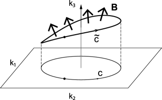
Figure 1: Trajectories in the parameter space. When we consider a periodic trajectory C in the $(k_{1},k_{2})$ plane, $k_{3}$ is changed accordingly and we have a closed contour $\tilde{\rm C}$. The current is determined by the magnetic field penetrating a surface $\tilde{S}$ specified by $\tilde{\rm C}=\partial\tilde{S}$.

Geometrical picture. The nonadiabatic part, Eq. (9), has a similar form to the adiabatic part, Eq. (8), which leads to a geometrical interpretation. Suppose that we control the system by using two time-dependent periodic parameters $\bm{k}(t)=(k_{1}(t),k_{2}(t))$. The adiabatic current $J_{\rm ad}$ arises only when the orbit of $\bm{k}$ encloses a finite area. The adiabatic current is represented by a flux penetrating the surface. This geometrical picture is also applied to the nonadiabatic part. We extend the parameter space and introduce a third axis $k_{3}=\delta_{2}$. Although $\delta_{2}$ is a function of $k_{1}$ and $k_{2}$, we leave it independent for the moment and use the relation after the calculation. In the extended space $\tilde{\bm{k}}=(\bm{k},k_{3})$, $J_{\rm g}$ is written as

$$J_{\rm g}=\oint_{\tilde{C}}\mathrm{d}\tilde{\bm{k}}\cdot\bm{A}(\bm{k})=\int_{\tilde{S}}\mathrm{d}\tilde{\bm{S}}(\tilde{\bm{k}})\cdot\bm{B}(\bm{k}),$$ (10)

where $\tilde{C}$ represents the closed contour in the $\tilde{\bm{k}}$ space and $\bm{A}(\bm{k})$ is the “gauge field”:

$$\bm{A}(\bm{k})=\frac{\omega}{2\pi}\left(\begin{array}[]{c}p^{\rm(R)}\partial_{1}p_{\rm out}\\ p^{\rm(R)}\partial_{2}p_{\rm out}\\ p^{\rm(R)}\end{array}\right).$$ (14)

This vector function is independent of $k_{3}$. The adiabatic part is represented by the first and second components of $\bm{A}$ and the nonadiabatic part is by the third component. We can introduce the corresponding “magnetic field” $\bm{B}(\bm{k})=\bm{\nabla}\times\bm{A}(\bm{k})$. The third (first and second) component of $\bm{B}(\bm{k})$ corresponds to the adiabatic (nonadiabatic) part. Using the Stokes theorem, we obtain the last expression in Eq. (10). The integral represents a surface integral where the surface $\tilde{S}$ is defined by using the closed contour $\tilde{C}$. This is pictorially represented as in Fig. 1. This surface is not unique and we can consider a convenient choice. This geometrical representation does not mean that the result is independent of the control speed. $\bm{B}$ is written in terms of purely geometric variables $k_{1}$ and $k_{2}$, but the third axis is determined by the dynamics.

Structure of the transition-rate matrix. Since the current is linear in $W$, the decomposition of the current can also be applied to the transition-rate matrix as $W(t)=W_{\rm d}(t)+W_{\rm g}(t)$. The explicit form of $W_{\rm g}(t)$ is given by

$$W_{\rm g}(t)=\left(\dot{p}_{\rm out}(t)+\dot{\delta}_{2}(t)\right)\left(\begin{array}[]{cc}1&1\\ -1&-1\end{array}\right).$$ (17)

The solution of the master equation $|p(t)\rangle$ is given by the adiabatic state of $W_{\rm d}(t)$. $W_{\rm g}(t)$ is interpreted as a counterdiabatic term known in shortcuts to adiabaticity (See SM) [50, 51, 52, 53, 54, 55]. It has a geometrical meaning [56], which is consistent with the geometrical interpretation for $J_{\rm g}$.

Using the decomposition of $W(t)$, we can also find a relation to the Floquet theory. The time-evolution operator $U(t)={\rm T}\exp\left(\int_{0}^{t}\mathrm{d}t^{\prime}\,W(t^{\prime})\right)$, where ${\rm T}$ is the time-ordering operator, is written at $t=T_{0}=2\pi/\omega$ as $U(T_{0})=\mathrm{e}^{T_{0}W_{\rm F}}$ to define the effective transition-rate matrix $W_{\rm F}$. Since the solution of the master equation is characterized as a stationary state of $W_{\rm F}$, $W_{\rm F}$ must be related to $W_{\rm d}(t)$. In fact, we can write

$$W_{\rm F}=\frac{\bar{k}}{k_{\rm in}(0)+k_{\rm out}(0)}\frac{W_{\rm d}(T_{0})-\mathrm{e}^{-2\pi\bar{k}/\omega}W_{\rm d}(0)}{1-\mathrm{e}^{-2\pi\bar{k}/\omega}},$$ (18)

where $\bar{k}=\frac{1}{T_{0}}\int_{0}^{T_{0}}\mathrm{d}t\,\left(k_{\rm in}(t)+k_{\rm out}(t)\right)$. See SM for details. In the adiabatic limit $\omega\to 0$, we find $W_{\rm F}\sim W_{\rm d}(T_{0})$, which is consistent with the above consideration. In the opposite limit, the function can be expanded in powers of $1/\omega$, which is equivalent to the Floquet–Magnus expansion [57, 58]. This relation is useful since we can find the decomposition of $W(t)$ by using the expansion at high frequencies.

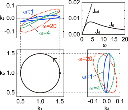
Figure 2: The frequency dependence of the current (top right) and trajectories in the parameter space at several values of $\omega$. We set $k_{1}=k_{\rm in}^{\rm(L)}(t)=k_{0}\left(1+\frac{1}{2}\cos\omega t\right)$, $k_{2}=k_{\rm in}^{\rm(R)}(t)=k_{0}\left(1+\frac{1}{2}\sin\omega t\right)$, $k_{\rm out}^{\rm(L)}=k_{0}$, and $k_{\rm out}^{\rm(R)}=k_{0}$. All the quantities are plotted in unit of $k_{0}$.

Nonadiabatic effects on geometric current. A typical behavior of the current is shown in Fig. 2. We use a similar protocol as used in Ref. [9]. Since we use a protocol with no net bias, the dynamical current is negligibly small. At low $\omega$, the adiabatic current is dominant, which is proportional to $\omega$. It is considerably disturbed by the nonadiabatic effects at high $\omega$. The total current approaches zero as $1/\omega$, as is found from the Floquet–Magnus expansion. Thus, the nonadiabatic effect inhibits the linearity of the geometric current with respect to $\omega$.

The behavior of the current is understood from the geometrical picture. Since the third component of the flux $B_{3}(\bm{k})=\partial_{1}A_{2}(\bm{k})-\partial_{2}A_{1}(\bm{k})$ determines the adiabatic current, the geometric current coincides with the adiabatic current if the trajectory $\tilde{\rm C}$ is parallel to the $(k_{1},k_{2})$ plane. In Fig. 2, we see that, as the frequency increases, the trajectory is distorted from a flat plane to cancel out the adiabatic part.

In Fig. 3, we plot the current when the trajectory ${\rm C}$ is slightly deformed while keeping the dynamical current invariant (See SM for details). We still observe nonadiabatic effects affecting linear growth. To keep the adiabatic current, we need to design the protocol such that the plane is kept parallel to the $(k_{1},k_{2})$ plane. Since we cannot choose the trajectory $\tilde{\rm C}$ arbitrary, this is a difficult problem in general.

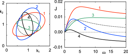
Figure 3: Left: Elliptic trajectories (1–4) keeping the dynamical current invariant. The dashed line represents the original protocol used in Fig. 2. Right: The corresponding total current. The dynamical part is zero in each protocol. See SM for details.

Assisted adiabatic pumping. To obtain a desirable enhancement of the geometric current, we use a method of counterdiabatic driving. We introduce the counterdiabatic term into the original transition matrix so that the adiabatic state of the original matrix becomes the exact solution. Although the idea is implemented for the Schrödinger equation for isolated quantum systems, the generalization to other equations such as the master equation and the Fokker–Planck equation is a straightforward task. We can find several applications in previous studies [59, 60, 61, 62].

In the master equation, the transition-rate matrix is diagonalized as $W(t)=\sum_{n}\epsilon_{n}(t)|\phi_{n}(t)\rangle\langle\phi_{n}(t)|$ and the adiabatic state is defined by Eq. (2) with time-independent coefficients $\{C_{n}\}$. We modify the transition-rate matrix $W(t)\to W(t)+W_{\rm CD}(t)$ so that the solution of the modified master equation is given by the adiabatic state. The counterdiabatic term $W_{\rm CD}(t)$ is given by

$$W_{\rm CD}(t)=\sum_{m,n(m\neq n)}|\phi_{m}(t)\rangle\langle\phi_{m}(t)|\dot{\phi}_{n}(t)\rangle\langle\phi_{n}(t)|.$$ (19)

For the two-state case, $W_{\rm CD}(t)$ can be explicitly written as

$$W_{\rm CD}(t)=\dot{p}_{\rm out}(t)\left(\begin{array}[]{cc}1&1\\ -1&-1\end{array}\right).$$ (22)

This form is slightly different from $W_{\rm g}(t)$ in Eq. (17). We see that the addition of the counterdiabatic term is obtained by replacements $k_{\rm in}(t)\to k_{\rm in}(t)-\dot{p}_{\rm out}(t)$ and $k_{\rm out}(t)\to k_{\rm out}(t)+\dot{p}_{\rm out}(t)$. Since these variables represent the transition rates, $|\dot{p}_{\rm out}(t)|$ cannot be large and the method fails for rapid changes of parameters.

The inclusion of the counterdiabatic term ensures that the exact solution of the master equation is given by the adiabatic state of the original transition-rate matrix. $k_{\rm in}(t)$ and $k_{\rm out}(t)$ are, respectively, represented by the sum of the left and right parts and we still have degrees of freedom to implement the counterdiabatic term. We can use them to keep the dynamical part of the current invariant and to set that the geometric part of the current is given by the adiabatic part of the original current without assist (See SM).

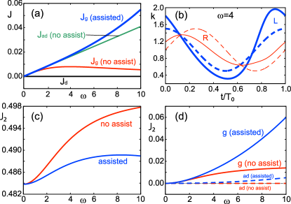
Figure 4: Assisted adiabatic pumping. We use the same protocol as used in Fig. 2 for the original system before assist. (a) The geometric current with an assisting field is represented by the blue line. The other lines are the same as in the top right panel of Fig. 2. (b) Dashed lines representing protocols before assist are changed to solid lines by the assisting field. Bold blue lines represent the left amplitude $k_{\rm in}^{\rm(L)}$ and thin red lines do the right amplitude $k_{\rm in}^{\rm(R)}$. We take $\omega=4.0$. (c) The current fluctuations before/after assist (See SM). (d) The geometric part (solid lines) and the adiabatic part (dashed lines) of the current fluctuations.

Although the above procedure works in principle, we have no clear picture on how the assisting field enhances the current. In addition, the manipulation is restricted in realistic situations and we cannot control each element in the transition-rate matrix independently. In our choice in the above examples, we set that $k_{\rm out}$ is time independent. The introduction of the counterdiabatic term inevitably breaks this condition. To keep the time independence of $k_{\rm out}$, we can consider scaling. After the introduction of the counterdiabatic term, we write the transition-rate matrix as

$$W(t)+W_{\rm CD}(t)=\left(1+\frac{\dot{p}_{\rm out}(t)}{k_{\rm out}}\right)\left(\begin{array}[]{cc}{\displaystyle-\frac{1-\frac{\dot{p}_{\rm out}(t)}{k_{\rm in}(t)}}{1+\frac{\dot{p}_{\rm out}(t)}{k_{\rm out}}}k_{\rm in}(t)}&k_{\rm out}\\ {\displaystyle\frac{1-\frac{\dot{p}_{\rm out}(t)}{k_{\rm in}(t)}}{1+\frac{\dot{p}_{\rm out}(t)}{k_{\rm out}}}k_{\rm in}(t)}&-k_{\rm out}\end{array}\right).$$ (25)

The prefactor of the right-hand side is positive and is scaled out by the redefinition of the timescale as $\mathrm{d}\tilde{t}=\mathrm{d}t(1+\dot{p}_{\rm out}(t)/k_{\rm out})$. We still have a degree of freedom to decompose the new component $k_{\rm in}(t)$ into the left and right parts and use it to keep the dynamical current invariant. In this case, the geometric current is not equal to the adiabatic current in the original system and is not proportional to the frequency. However, we confirm that the deviation is not so large and the geometric current can be kept growing as a function of the frequency. The result is shown in Fig. 4 (See SM for details). The obtained protocol indicates that we need to shift the oscillation of the assisting field to the left compared to the original one to prevent the deviation. The required field becomes larger when we consider faster driving and the control fails at some frequency where $|\dot{p}_{\rm out}(t)|$ exceeds the threshold.

In Fig. 4, we also plot the current fluctuation that is decreasing by the introduction of the assisting field. Generally, the counterdiabatic term leads to an increase in the energy cost characterized by the fluctuation and a broadening of the work distribution [63, 64]. This expectation i.e. the increment of the fluctuation for the geometric part under the assisting field is verified as can be seen on the bottom right panel of Fig. 4. Although we cannot control the dynamical part of the fluctuation as we did for the average, we find a decrease of the total fluctuation as a result of the decrease of the dynamical fluctuation. The suppression of the fluctuations implies the stability of the assisted driving. A variational formulation of the counterdiabatic driving for quantum systems also indicates a stable driving [65]. In SM, we examine several examples to confirm the stability by slightly modifying the amplitudes in several ways.

Note added in proof. After the completion of this work, we learned about Ref. [66] where a similar method is used for adiabatic pumping.

We are grateful to Adolfo del Campo, Ken Funo, Jun Ohkubo, and Keiji Saito for useful discussions and comments. We also thank Ville Paasonen for his critical reading of this manuscript. This work was supported by JSPS KAKENHI Grant No. JP19J13698 (K. F.), No. JP16H04025 (H. H. and Y. H.), and No. JP26400385 (K. T.). K. T. acknowledges the warm hospitality of the Yukawa Institute for Theoretical Physics, Kyoto University during his stay there to promote the collaboration among the authors.

I Supplemental Material

II Master equation

II.1 Improved adiabatic approximation

We want to solve the master equation

$$\frac{\mathrm{d}}{\mathrm{d}t}|p(t)\rangle=W(t)|p(t)\rangle.$$ (S1)

We assume that the matrix is diagonalizable. Then, the instantaneous eigenstates of $W(t)$ are prepared as

$$W(t)|\phi_{n}(t)\rangle=\epsilon_{n}(t)|\phi_{n}(t)\rangle,$$ (S2)

$$\langle\phi_{n}(t)|W(t)=\langle\phi_{n}(t)|\epsilon_{n}(t).$$ (S3)

We have the orthonormal relations and the resolution of unity:

$$\langle\phi_{m}(t)|\phi_{n}(t)\rangle=\delta_{m,n},$$ (S4)

$$\sum_{n}|\phi_{n}(t)\rangle\langle\phi_{n}(t)|=1.$$ (S5)

The left and the right eigenstates are not a simple conjugate with each other. We also assume that $n=1$ represents the stationary state and the other states represent decaying contributions, which means that the eigenvalues satisfy

$$\epsilon_{1}(t)=0,$$ (S6)

$$\epsilon_{n}(t)<0\quad(n\neq 1).$$ (S7)

Although it is difficult to find a specific form of the eigenstates in general, $\langle\phi_{1}(t)|$ has a simple form as

$$\langle\phi_{1}(t)|=\left(\begin{array}[]{cccc}1&1&\cdots&1\end{array}\right)=:\langle 1|,$$ (S9)

due to the property of the transition-rate matrix $\sum_{i}W_{ij}(t)=0$.

The eigenstates have degrees of freedom as

$$|\phi_{n}(t)\rangle\to R_{n}(t)|\phi_{n}(t)\rangle,$$ (S10)

$$\langle\phi_{n}(t)|\to\langle\phi_{n}(t)|R_{n}^{-1}(t),$$ (S11)

where $R_{n}(t)$ is an arbitrary function with $R_{n}(0)=1$. To remove this arbitrariness, we introduce

$$|\tilde{\phi}_{n}(t)\rangle=\mathrm{e}^{-\int_{0}^{t}\mathrm{d}t^{\prime}\,\langle\phi_{n}(t^{\prime})|\dot{\phi}_{n}(t^{\prime})\rangle}|\phi_{n}(t)\rangle,$$ (S12)

$$\langle\tilde{\phi}_{n}(t)|=\langle\phi_{n}(t)|\mathrm{e}^{\int_{0}^{t}\mathrm{d}t^{\prime}\,\langle\phi_{n}(t^{\prime})|\dot{\phi}_{n}(t^{\prime})\rangle}.$$ (S13)

These eigenstates are invariant under the transformation of $R_{n}(t)$. We note that the transformation does not change the properties in Eqs. (S4) and (S5). We also have for any $n$

$$\langle\tilde{\phi}_{n}(t)|\dot{\tilde{\phi}}_{n}(t)\rangle=0.$$ (S14)

We expand the solution of the master equation with respect to $\{|\tilde{\phi}_{n}(t)\rangle\}$ as

$$|p(t)\rangle=\sum_{n}C_{n}(t)\mathrm{e}^{\int_{0}^{t}\mathrm{d}t^{\prime}\,\epsilon_{n}(t^{\prime})}|\tilde{\phi}_{n}(t)\rangle.$$ (S15)

$C_{1}(t)$ is determined from the normalization as

$$C_{1}(t)=\langle\tilde{\phi}_{1}(t)|p(t)\rangle=\langle 1|p(t)\rangle=1.$$ (S16)

To solve the other components, we substitute the representation (S15) to the master equation and multiply $\langle\tilde{\phi}_{n}(t)|$ from the left. We obtain

$$\sum_{m(\neq 1)}C_{m}(t)\mathrm{e}^{\int_{0}^{t}\mathrm{d}t^{\prime}\,\epsilon_{m}(t^{\prime})}\langle\tilde{\phi}_{1}(t)|\dot{\tilde{\phi}}_{m}(t)\rangle=0,$$ (S17)

$$\frac{\mathrm{d}C_{n}(t)}{\mathrm{d}t}\mathrm{e}^{\int_{0}^{t}\mathrm{d}t^{\prime}\,\epsilon_{n}(t^{\prime})}+\langle\tilde{\phi}_{n}(t)|\dot{\tilde{\phi}}_{1}(t)\rangle$$

$$+\sum_{m(\neq 1,n)}C_{m}(t)\mathrm{e}^{\int_{0}^{t}\mathrm{d}t^{\prime}\,\epsilon_{m}(t^{\prime})}\langle\tilde{\phi}_{n}(t)|\dot{\tilde{\phi}}_{m}(t)\rangle=0.$$ (S18)

In the second equation, the contribution of $m=1$ is separated from the sum.

As we mention in the main body of the paper, we neglect the third term on the left hand side of Eq. (S18). Then, we obtain

$$C_{n}(t)\simeq C_{n}(0)-\int_{0}^{t}\mathrm{d}t^{\prime}\,\langle\tilde{\phi}_{n}(t^{\prime})|\dot{\tilde{\phi}}_{1}(t^{\prime})\rangle\mathrm{e}^{-\int_{0}^{t^{\prime}}\mathrm{d}t^{\prime\prime}\,\epsilon_{n}(t^{\prime\prime})}.$$ (S19)

The solution of the master equation is approximated to

$$|p(t)\rangle\simeq|\tilde{\phi}_{1}(t)\rangle+\sum_{n(\neq 1)}\left(\delta_{n}(t)+C_{n}(0)\mathrm{e}^{\int_{0}^{t}\mathrm{d}t^{\prime}\,\epsilon_{n}(t^{\prime})}\right)|\tilde{\phi}_{n}(t)\rangle,$$

where

$$\delta_{n}(t)=-\int_{0}^{t}\mathrm{d}t^{\prime}\,\langle\tilde{\phi}_{n}(t^{\prime})|\dot{\tilde{\phi}}_{1}(t^{\prime})\rangle\mathrm{e}^{\int_{t^{\prime}}^{t}\mathrm{d}t^{\prime\prime}\,\epsilon_{n}(t^{\prime\prime})}.$$ (S21)

II.2 Exact solution for two-state system

To obtain an explicit form of the state, we examine the two-state case. The transition-rate matrix is generally written as

$$W(t)=\left(\begin{array}[]{cc}-k_{\rm in}(t)&k_{\rm out}(t)\\ k_{\rm in}(t)&-k_{\rm out}(t)\end{array}\right),$$ (S24)

where $k_{\rm in}(t)$ and $k_{\rm out}(t)$ are arbitrary nonnegative functions. The instantaneous eigenstates of $W(t)$ are given by

$$\{|\phi_{n}(t)\rangle\}_{n=1,2}=\left\{\left(\begin{array}[]{c}p_{\rm out}(t)\\ 1-p_{\rm out}(t)\end{array}\right),\quad\left(\begin{array}[]{c}1\\ -1\end{array}\right)\right\},$$ (S29)

$$\{\langle\phi_{n}(t)|\}_{n=1,2}=\left\{\left(\begin{array}[]{cc}1&1\end{array}\right),\quad\left(\begin{array}[]{cc}1-p_{\rm out}(t)&-p_{\rm out}(t)\end{array}\right)\right\},$$ (S32)

where

$$p_{\rm out}(t)=\frac{k_{\rm out}(t)}{k_{\rm in}(t)+k_{\rm out}(t)}.$$ (S34)

The corresponding eigenvalues are $\{\epsilon_{n}(t)\}_{n=1,2}=\{0,-(k_{\rm in}(t)+k_{\rm out}(t))\}$. The component $n=1$ represents the instantaneous stationary state. In this case, the geometric phase is zero in each level and we have $|\tilde{\phi}_{n}(t)\rangle=|\phi_{n}(t)\rangle$ and $\langle\tilde{\phi}_{n}(t)|=\langle\phi_{n}(t)|$.

Now we expand the solution as in Eq. (S15). Using the master equation, we obtain

$$\frac{\mathrm{d}C_{1}(t)}{\mathrm{d}t}=0,$$ (S35)

$$\frac{\mathrm{d}C_{2}(t)}{\mathrm{d}t}=-C_{1}(t)\mathrm{e}^{\int_{0}^{t}\mathrm{d}t^{\prime}\,(\epsilon_{1}(t^{\prime})-\epsilon_{2}(t^{\prime}))}\langle\phi_{2}(t)|\dot{\phi}_{1}(t)\rangle.$$ (S36)

The first equation shows that $C_{1}$ is independent of $t$, and the second equation can be solved simply by integrating the equation. With the initial condition $|p(0)\rangle=(p_{0},1-p_{0})^{\rm T}$, we obtain the exact result:

$$|p(t)\rangle = \left(\begin{array}[]{c}p_{\rm out}(t)+\delta(t)\\ 1-p_{\rm out}(t)-\delta(t)\end{array}\right)$$ (S42)

$$+\left(p_{0}-p_{\rm out}(0)\right)\mathrm{e}^{-\int_{0}^{t}\mathrm{d}t^{\prime}\,(k_{\rm in}(t^{\prime})+k_{\rm out}(t^{\prime}))}\left(\begin{array}[]{c}1\\ -1\end{array}\right),$$

where

$$\delta(t)=-\int_{0}^{t}\mathrm{d}t^{\prime}\,\dot{p}_{\rm out}(t^{\prime})\mathrm{e}^{-\int_{t^{\prime}}^{t}\mathrm{d}t^{\prime\prime}\,(k_{\rm in}(t^{\prime\prime})+k_{\rm out}(t^{\prime\prime}))}.$$ (S43)

$\delta(t)$ is equivalent to $\delta_{n}(t)$ in Eq. (S21) with $n=2$. The dependence of the initial condition is only in the last term of Eq. (S42). This term decays exponentially as a function of $t$. Combining with the property of $\delta(t)$ discussed below, we can conclude that the system rapidly approaches a periodic behavior which is independent of the initial condition and the pumping current is independent of the second term of Eq. (S42).

Generally, the time evolution operator between two states, defined by $|p(t_{2})\rangle=U(t_{2},t_{1})|p(t_{1})\rangle$, is given by

$$U(t_{2},t_{1})=|\phi_{1}(t_{2})\rangle\langle 1|+\delta(t_{2})|2\rangle\langle 1|$$

$$+\mathrm{e}^{-\int_{t_{1}}^{t_{2}}\mathrm{d}t\,(k_{\rm in}(t)+k_{\rm out}(t))}\left(|2\rangle\langle\phi_{2}(t_{1})|-\delta(t_{1})|2\rangle\langle 1|\right),$$ (S44)

where $|2\rangle=|\phi_{2}(t)\rangle$ is independent of $t$. This operator can be written in a matrix form as

$$U(t_{2},t_{1}) = 1+\frac{W_{\rm d}(t_{2})}{k_{\rm in}(t_{2})+k_{\rm out}(t_{2})}$$ (S45)

$$-\mathrm{e}^{-\int_{t_{1}}^{t_{2}}\mathrm{d}t\,(k_{\rm in}(t)+k_{\rm out}(t))}\frac{W_{\rm d}(t_{1})}{k_{\rm in}(t_{1})+k_{\rm out}(t_{1})},$$

where

$$\frac{W_{\rm d}(t)}{k_{\rm in}(t)+k_{\rm out}(t)}=\left(\begin{array}[]{cc}-(1-p_{\rm out}(t)-\delta(t))&p_{\rm out}(t)+\delta(t)\\ 1-p_{\rm out}(t)-\delta(t)&-(p_{\rm out}(t)+\delta(t))\end{array}\right).$$ (S48)

(S49)

In the following calculations, we use the time-evolution operator to obtain the current fluctuations and the Floquet transition-rate matrix.

III On the behavior of $\delta(t)$

The nonadiabatic effects are determined by $\delta_{n}(t)$ in Eq. (S21). Since the structure of the function is unchanged for any choice of $n$, we study the two-state case with $n=2$. $\delta(t)=\delta_{2}(t)$ defined in Eq. (S43) satisfies the differential equation

$$\frac{\mathrm{d}\delta(t)}{\mathrm{d}t}=-(k_{\rm in}(t)+k_{\rm out}(t))\left(\delta(t)+\frac{\dot{p}_{\rm out}(t)}{k_{\rm in}(t)+k_{\rm out}(t)}\right).$$ (S1)

We see that $\delta(t)=\delta^{(0)}(t)$ with $\delta^{(0)}(t):=-\dot{p}_{\rm out}(t)/(k_{\rm in}(t)+k_{\rm out}(t))$ represents the stationary point. This point is stable against the deviation. Therefore, if $p_{\rm out}(t)$ changes very slowly, $\delta(t)\simeq\delta^{(0)}(t)$ becomes a good approximation.

To improve the approximation, we consider the derivative expansion. Equation (S1) is rewritten as

$$\delta(t)=\delta^{(0)}(t)-\frac{1}{k_{\rm in}(t)+k_{\rm out}(t)}\frac{\mathrm{d}}{\mathrm{d}t}\delta(t).$$ (S2)

Solving the equation recursively, we obtain

$$\delta(t) = \delta^{(0)}(t)+\left(-\frac{1}{k_{\rm in}(t)+k_{\rm out}(t)}\frac{\mathrm{d}}{\mathrm{d}t}\right)\delta^{(0)}(t)$$ (S3)

$$+\left(-\frac{1}{k_{\rm in}(t)+k_{\rm out}(t)}\frac{\mathrm{d}}{\mathrm{d}t}\right)^{2}\delta^{(0)}(t)+\cdots.$$

When each parameter is written as a function of $\omega t$, this is a series expansion of $\omega$ for a fixed $\omega t$. The first term is the first order in $\omega$, the second term is the second order, and so on.

We plot $\delta(t)$ in Fig. 5. We consider the following periodic driving:

$$k_{\rm in}^{\rm(L)}(t)=k_{0}\left(1+\frac{1}{2}\cos\omega t\right),$$ (S4)

$$k_{\rm in}^{\rm(R)}(t)=k_{0}\left(1+\frac{1}{2}\sin\omega t\right),$$ (S5)

$$k_{\rm out}^{\rm(L)}(t)=k_{0},$$ (S6)

$$k_{\rm out}^{\rm(R)}(t)=k_{0}.$$ (S7)

$k_{0}$ represents a constant. As we see in the figure, $\delta(t)$ is almost periodic in $t$ for any choice of parameters. It can be approximated to the stationary value $\delta^{(0)}(t)$ at small-$\omega$. The deviation is described by the expansion in Eq. (S3).

In the opposite limit where $\omega$ is large, $\delta(t)$ is approximated to $-(p_{\rm out}(t)-p_{\rm out}(0))$. This is obtained by neglecting $\delta(t)$ in the right hand side of Eq. (S1). The $1/\omega$-correction can be evaluated by using the Floquet–Magnus expansion.

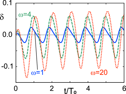
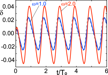
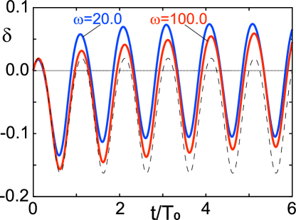
Figure 5: Top: $\delta(t)$ for several values of $\omega$. Bottom Left: $\delta(t)$ for a slow driving (small $\omega$). $\delta(t)$ at $\omega=1.0$ is denoted by the blue solid line and $\omega=2.0$ by the red solid line. The black dashed line denotes the stationary point $\delta^{(0)}(t)=-\dot{p}_{\rm out}(t)/(k_{\rm in}(t)+k_{\rm out}(t))$. Bottom Right: $\delta(t)$ for a fast driving (large $\omega$). $\delta(t)$ at $\omega=20.0$ is denoted by the blue solid line and $\omega=100.0$ by the red solid line. The black dashed line denotes the asymptotic result $\delta(t)\simeq-p_{\rm out}(t)+p_{\rm out}(0)$.

IV Counting field and current distributions

IV.1 Counting field

The current distribution function is calculated by introducing the counting field $\chi$ to the transition-rate matrix as $W(t)\to W(t;\chi)$. The explicit form is given by

$$W(t;\chi)=\left(\begin{array}[]{cc}-k_{\rm in}(t)&k_{\rm out}^{\rm(L)}(t)+k_{\rm out}^{\rm(R)}(t)\mathrm{e}^{i\chi}\\ k_{\rm in}^{\rm(L)}(t)+k_{\rm in}^{\rm(R)}(t)\mathrm{e}^{-i\chi}&-k_{\rm out}(t)\end{array}\right).$$ (S3)

Using the solution of the master equation $|p(t;\chi)\rangle$ with the modified matrix $W(t;\chi)$, we write

$$\langle 1|p(t;\chi)\rangle=\exp\left(i\chi n(t)-\frac{\chi^{2}}{2}n_{2}(t)+\cdots\right),$$ (S5)

and the average current and the fluctuation is given by

$$J=\lim_{T\to\infty}\frac{1}{T}n(T),$$ (S6)

$$J_{2}=\lim_{T\to\infty}\frac{1}{T}n_{2}(T).$$ (S7)

We note that $J_{2}$ represents the second-order cumulant $\langle\hat{J}^{2}\rangle-\langle\hat{J}\rangle^{2}$.

To calculate the current distributions, we expand the matrix $W(t;\chi)$ as

$$W(t;\chi)=W(t)+i\chi V_{1}(t)-\frac{\chi^{2}}{2}V_{2}(t)+\cdots,$$ (S8)

$$V_{1}(t)=\left(\begin{array}[]{cc}0&k_{\rm out}^{\rm(R)}(t)\\ -k_{\rm in}^{\rm(R)}(t)&0\end{array}\right),$$ (S11)

$$V_{2}(t)=\left(\begin{array}[]{cc}0&k_{\rm out}^{\rm(R)}(t)\\ k_{\rm in}^{\rm(R)}(t)&0\end{array}\right).$$ (S14)

IV.2 Current distributions

Using the derived formula, we find that the average current is given by

$$J = \lim_{T\to\infty}\frac{1}{T}\int_{0}^{T}\mathrm{d}t\,\langle 1|V_{1}(t)|p(t)\rangle$$ (S15)

$$= \lim_{T\to\infty}\frac{1}{T}\int_{0}^{T}\mathrm{d}t\,\left(k_{\rm out}^{\rm(R)}(t)p_{2}(t)-k_{\rm in}^{\rm(R)}(t)p_{1}(t)\right).$$

Using Eq. (S42), we have

$$J = \lim_{T\to\infty}\frac{1}{T}\int_{0}^{T}\mathrm{d}t\,\Bigl{[}k_{\rm out}^{\rm(R)}(t)(1-p_{\rm out}(t))-k_{\rm in}^{\rm(R)}(t)p_{\rm out}(t)$$ (S16)

$$-\left(k_{\rm out}^{\rm(R)}(t)+k_{\rm in}^{\rm(R)}(t)\right)\delta(t)\Bigr{]}.$$

Since the second term of Eq. (S42) incorporates an exponential factor, it does not contribute to the result. Then, we find that the current is independent on the initial condition. The dynamical part of the current is given by setting $\delta(t)=0$. The decomposition of the geometric part into the adiabatic part and the nonadiabatic part can be found by using Eq. (S2). The explicit form of each part is given in the main body of the paper.

Similarly, the fluctuation is obtained from

$$-\frac{1}{2}\left(n_{2}(t)+n^{2}(t)\right)=-\frac{1}{2}\int_{0}^{t}\mathrm{d}t^{\prime}\,\langle 1|V_{2}(t^{\prime})|p(t^{\prime})\rangle$$

$$-\int_{0}^{t}\mathrm{d}t_{2}\int_{0}^{t_{2}}\mathrm{d}t_{1}\,\langle 1|V_{1}(t_{2})U(t_{2},t_{1})V_{1}(t_{1})|p(t_{1})\rangle.$$ (S17)

After some calculations, we obtain

$$J_{2}=\lim_{T\to\infty}\frac{1}{T}\int_{0}^{T}\mathrm{d}t\,\Bigl{[}k_{\rm out}^{\rm(R)}(t)p_{\rm in}(t)+k_{\rm in}^{\rm(R)}(t)p_{\rm out}(t)$$

$$-\left(k_{\rm out}^{\rm(R)}(t)-k_{\rm in}^{\rm(R)}(t)\right)\delta(t)+2\left(k_{\rm out}^{\rm(R)}(t)+k_{\rm in}^{\rm(R)}(t)\right)\Delta(t)\Bigr{]},$$ (S18)

where

$$\Delta(t)=-\int_{0}^{t}\mathrm{d}t^{\prime}\,\Bigl{[}k_{\rm out}^{\rm(R)}(t^{\prime})(p_{\rm in}(t^{\prime})-\delta(t^{\prime}))^{2}$$

$$+k_{\rm in}^{\rm(R)}(t^{\prime})(p_{\rm out}(t^{\prime})+\delta(t^{\prime}))^{2}\Bigr{]}\mathrm{e}^{-\int_{t^{\prime}}^{t}\mathrm{d}t^{\prime\prime}\,(k_{\rm in}(t^{\prime\prime})+k_{\rm out}(t^{\prime\prime}))}.$$ (S19)

$\Delta(t)$ satisfies a first-order differential equation which has a similar form to that for $\delta(t)$ and its behavior can also be understood in a similar way. It is a straightforward task to decompose $J_{2}$ into dynamical, adiabatic, and nonadiabatic parts and we do not show their explicit forms here.

V Decomposition of the transition-rate matrix

In the time-evolution operator, we have introduced a matrix $W_{\rm d}(t)$ in Eq. (S49). It satisfies the eigenvalue equations

$$W_{\rm d}(t)\left(\begin{array}[]{c}p_{\rm out}(t)+\delta(t)\\ 1-p_{\rm out}(t)-\delta(t)\end{array}\right)=0,$$ (S3)

$$W_{\rm d}(t)\left(\begin{array}[]{c}1\\ -1\end{array}\right)=-(k_{\rm in}(t)+k_{\rm out}(t))\left(\begin{array}[]{c}1\\ -1\end{array}\right).$$ (S8)

Each vector appears in the solution of the master equation (S42). This property shows that $|p(t)\rangle$ is equal to the adiabatic state of $W_{\rm d}(t)$. Then, $W(t)$ is decomposed as

$$W(t)=W_{\rm d}(t)+W_{\rm g}(t),$$ (S9)

and $W_{\rm g}(t)$ plays the role of the counterdiabatic term. Using Eq. (S1), we can write $W_{\rm g}(t)$ as

$$W_{\rm g}(t)=(\dot{p}_{\rm out}(t)+\dot{\delta}(t))\left(\begin{array}[]{cc}1&1\\ -1&-1\end{array}\right).$$ (S12)

This term gives the geometric current as we see from the relation

$$(W_{\rm g}(t))_{12}^{\rm(R)}p_{2}(t)-(W_{\rm g}(t))_{21}^{\rm(R)}p_{1}(t)=p^{\rm(R)}(t)\left(\dot{p}_{\rm out}(t)+\dot{\delta}(t)\right).$$

VI Floquet theory

We derive the Floquet effective transition-rate matrix $W_{\rm F}$ defined as

$$U(T_{0},0)=\mathrm{e}^{T_{0}W_{\rm F}}.$$ (S1)

The time-evolution operator is given in Eq. (S45). It has a form

$$U(t_{2},t_{1})=1+X(t_{2},t_{1}),$$ (S2)

and the matrix $X$ satisfies the relation

$$X^{2}(t_{2},t_{1})=-\left(1-\mathrm{e}^{-\int_{t_{1}}^{t_{2}}\mathrm{d}t\,(k_{\rm in}(t)+k_{\rm out}(t))}\right)X(t_{2},t_{1}).$$ (S3)

This is a very convenient formula to take the logarithm of $U$. We easily find

$$W_{\rm F}T_{0} = \frac{\int_{0}^{T_{0}}\mathrm{d}t\,(k_{\rm in}(t)+k_{\rm out}(t))}{1-\mathrm{e}^{-\int_{0}^{T_{0}}\mathrm{d}t\,(k_{\rm in}(t)+k_{\rm out}(t))}}\frac{1}{k_{\rm in}(0)+k_{\rm out}(0)}$$ (S4)

$$\times\left(W_{\rm d}(T_{0})-\mathrm{e}^{-\int_{0}^{T_{0}}\mathrm{d}t\,(k_{\rm in}(t)+k_{\rm out}(t))}W_{\rm d}(0)\right).$$

To make the frequency dependence clear, we use

$$\bar{k}=\frac{1}{T_{0}}\int_{0}^{T_{0}}\mathrm{d}t\,\left(k_{\rm in}(t)+k_{\rm out}(t)\right),$$ (S5)

to write

$$W_{\rm F}=\bar{k}\left[\left(\begin{array}[]{cc}-p_{\rm in}(0)&p_{\rm out}(0)\\ p_{\rm in}(0)&-p_{\rm out}(0)\end{array}\right)+\frac{\delta(T_{0})}{1-\mathrm{e}^{-2\pi\bar{k}/\omega}}\left(\begin{array}[]{cc}1&1\\ -1&-1\end{array}\right)\right].$$ (S10)

We note that this is the exact form of the effective transition-rate matrix. The expression can be expanded in powers of $1/\omega$. We use the asymptotic expansion $\delta(t)\sim-(p_{\rm out}(t)-p_{\rm out}(0))+\cdots$. At the leading order, we have

$$W_{\rm F}\sim\frac{1}{T_{0}}\int_{0}^{T_{0}}\mathrm{d}t\,W(t).$$ (S12)

This is the zeroth order contribution in the Floquet–Magnus expansion, though Hamiltonian in the conventional Floquet–Magnus theory is replaced by the transition-rate matrix. Similarly, we can find the higher-order contributions.

VII Deformation of the protocol trajectory

The local dynamical current is given by

$$J_{\rm d}(t)=\frac{k_{\rm in}^{\rm(L)}(t)k_{\rm out}^{\rm(R)}(t)-k_{\rm out}^{\rm(L)}(t)k_{\rm in}^{\rm(R)}(t)}{k(t)}.$$ (S1)

We can easily confirm that $J_{\rm d}(t)$ is invariant under the transformation

$$k_{\rm in}^{\rm(L)}(t)\to k_{\rm in}^{\rm(L)}(t)+k^{\rm(L)}(t)f(t),$$ (S2)

$$k_{\rm in}^{\rm(R)}(t)\to k_{\rm in}^{\rm(R)}(t)+k^{\rm(R)}(t)f(t),$$ (S3)

where $k^{\rm(L)}=k_{\rm in}^{\rm(L)}+k_{\rm out}^{\rm(L)}$, $k^{\rm(R)}=k_{\rm in}^{\rm(R)}+k_{\rm out}^{\rm(R)}$, and $f(t)$ is an arbitrary function.

To keep the average of $k_{\rm in}(t)$ over the period, the average of $(k^{\rm(L)}(t)+k^{\rm(R)}(t))f(t)$ must be kept zero. One of the simplest choice is:

$$f(t)=\frac{k_{0}}{2}\frac{x\cos\omega t+y\sin\omega t}{k^{\rm(L)}(t)+k^{\rm(R)}(t)}.$$ (S4)

We show the protocols and the corresponding current in Fig. 3 of the main body of the paper. We set $(x,y)=(1.0,0.0)$ for the protocol 1, $(x,y)=(0.0,1.0)$ for 2, $(x,y)=(0.0,-1.0)$ for 3, and $(x,y)=(-1.0,0.0)$ for 4. The dynamical current is zero in all the protocols.

VIII Assisted adiabatic pumping

VIII.1 Choice of transition rates

We obtained in the main body of the paper that the assisted adiabatic driving is achieved by using the replacement

$$k_{\rm in}(t)\to k_{\rm in}(t)-\dot{p}_{\rm out}(t),$$ (S1)

$$k_{\rm out}(t)\to k_{\rm out}(t)+\dot{p}_{\rm out}(t),$$ (S2)

where the dot denotes the time derivative. This does not determine the decomposition of the left and right parts of the transition rates uniquely. We show in the following that we can find the ideal driving by

$$k_{\rm in}^{\rm(L)}\to k_{\rm in}^{\rm(L)}-\frac{k^{(\rm L)}_{\rm in}+k^{(\rm L)}_{\rm out}}{k}\dot{p}_{\rm out},$$ (S3)

$$k_{\rm in}^{\rm(R)}\to k_{\rm in}^{\rm(R)}-\frac{k^{(\rm R)}_{\rm in}+k^{(\rm R)}_{\rm out}}{k}\dot{p}_{\rm out},$$ (S4)

$$k_{\rm out}^{\rm(L)}\to k_{\rm out}^{\rm(L)}+\frac{k^{(\rm L)}_{\rm in}+k^{(\rm L)}_{\rm out}}{k}\dot{p}_{\rm out},$$ (S5)

$$k_{\rm out}^{\rm(R)}\to k_{\rm out}^{\rm(R)}+\frac{k^{(\rm R)}_{\rm in}+k^{(\rm R)}_{\rm out}}{k}\dot{p}_{\rm out},$$ (S6)

where $k=k_{\rm in}^{\rm(L)}+k_{\rm in}^{\rm(R)}+k_{\rm out}^{\rm(L)}+k_{\rm out}^{\rm(R)}$.

The local dynamical current in Eq. (S1) is invariant under the above transformation. The local geometric current is given by

$$J_{\rm g}(t)=\frac{k^{\rm(R)}(t)}{k(t)}\frac{\mathrm{d}}{\mathrm{d}t}\left(p_{\rm out}(t)+\delta(t)\right).$$ (S7)

$k^{\rm(R)}(t)/k(t)$ is invariant under the transformation. $p_{\rm out}(t)$ is changed as

$$p_{\rm out}(t)\to p_{\rm out}(t)+\frac{\dot{p}_{\rm out}(t)}{k(t)}.$$ (S8)

We also see from the integral form in Eq. (S43) that $\delta(t)$ is changed as

$$\delta(t) \to \delta(t)-\int_{0}^{t}\mathrm{d}t^{\prime}\,\frac{\mathrm{d}}{\mathrm{d}t^{\prime}}\left(\frac{\dot{p}_{\rm out}(t^{\prime})}{k(t^{\prime})}\right)\mathrm{e}^{-\int_{t^{\prime}}^{t}\mathrm{d}t^{\prime\prime}\,(k_{\rm in}(t^{\prime\prime})+k_{\rm out}(t^{\prime\prime}))}$$ (S9)

$$= -\frac{\dot{p}_{\rm out}(t)}{k(t)}+\frac{\dot{p}_{\rm out}(0)}{k(0)}\mathrm{e}^{-\int_{0}^{t}\mathrm{d}t^{\prime}\,(k_{\rm in}(t^{\prime})+k_{\rm out}(t^{\prime}))},$$

where we use the partial integration. The last term is a decaying function and does not contribute to the current. Then, we find

$$J_{\rm g}\to\frac{k^{\rm(R)}(t)}{k(t)}\frac{\mathrm{d}}{\mathrm{d}t}p_{\rm out}(t),$$ (S10)

which shows that the geometric current in the assisted system including nonadiabatic effects is equal to the adiabatic current in the original system.

VIII.2 Scaling

Suppose that we have a time-independent $k_{\rm out}$ and want to keep that value after introducing the counterdiabatic term. Using the time scaling

$$\tilde{t}(t)=\int_{0}^{t}\mathrm{d}t^{\prime}\,\left(1+\frac{\dot{p}_{\rm out}(t^{\prime})}{k_{\rm out}}\right),$$ (S11)

we obtain the master equation

$$\frac{\mathrm{d}}{\mathrm{d}\tilde{t}}|\tilde{p}(\tilde{t})\rangle=\tilde{W}(\tilde{t})|\tilde{p}(\tilde{t})\rangle,$$ (S12)

where

$$\tilde{W}(\tilde{t})=\left(\begin{array}[]{cc}-\tilde{k}_{\rm in}(\tilde{t})&k_{\rm out}\\ \tilde{k}_{\rm in}(\tilde{t})&-k_{\rm out}\end{array}\right),$$ (S15)

and

$$\tilde{k}_{\rm in}(\tilde{t})=\frac{1-\frac{\dot{p}_{\rm out}(t)}{k_{\rm in}(t)}}{1+\frac{\dot{p}_{\rm out}(t)}{k_{\rm out}}}k_{\rm in}(t).$$ (S16)

Since $\tilde{t}$ is different from $t$, the state at the scaled time $\tilde{t}$, $|\tilde{p}(\tilde{t})\rangle$, is the adiabatic state at the original scale $t$. We note that there is one-to-one correspondence between $t$ and $\tilde{t}$. To keep the dynamical current invariant, we can use the decomposition $\tilde{k}_{\rm in}(t)=\tilde{k}_{\rm in}^{\rm(L)}(t)+\tilde{k}_{\rm in}^{\rm(R)}(t)$ where

$$\tilde{k}_{\rm in}^{\rm(L)}=\frac{k_{\rm in}-\dot{p}_{\rm out}}{k_{\rm out}+\dot{p}_{\rm out}}k_{\rm out}^{\rm(L)}+\frac{k_{\rm in}^{\rm(L)}k_{\rm out}^{\rm(R)}-k_{\rm out}^{\rm(L)}k_{\rm in}^{\rm(R)}}{\left(k_{\rm out}+\dot{p}_{\rm out}\right)^{2}}k_{\rm out},$$ (S17)

$$\tilde{k}_{\rm in}^{\rm(R)}=\frac{k_{\rm in}-\dot{p}_{\rm out}}{k_{\rm out}+\dot{p}_{\rm out}}k_{\rm out}^{\rm(R)}-\frac{k_{\rm in}^{\rm(L)}k_{\rm out}^{\rm(R)}-k_{\rm out}^{\rm(L)}k_{\rm in}^{\rm(R)}}{\left(k_{\rm out}+\dot{p}_{\rm out}\right)^{2}}k_{\rm out}.$$ (S18)

The obtained protocol is shown in Fig. 6 for a slow driving and 7 for a fast driving. The obtained current is shown in Fig. 4 in the main body of the paper.

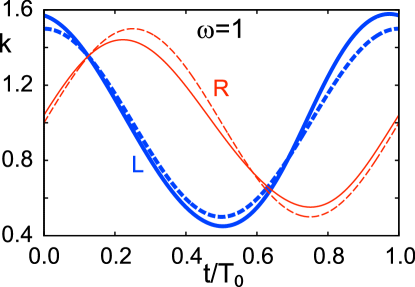
Figure 6: Protocols before/after the assist for $\omega=1.0$ . Top: Trajectories in parameter space. Dashed lines represent trajectories of the original protocol and solid lines of protocol with assist. Bottom: Time dependence of the protocols. Bold blue lines represent the left amplitude $k_{\rm in}^{\rm(L)}$ and thin red lines the right amplitude $k_{\rm in}^{\rm(R)}$. Dashed lines represent protocols before assist and solid lines with assist.

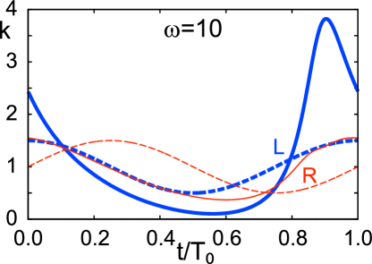
Figure 7: Protocols before/after the assist for $\omega=10.0$.

VIII.3 Stability

To examine the stability of the assisted driving, we consider small deviations from the ideal driving. We put

$$\tilde{k}_{\rm in}^{\rm(L)}\to\tilde{k}_{\rm in}^{\rm(L)}+\delta k,$$ (S19)

$$\tilde{k}_{\rm in}^{\rm(R)}\to\tilde{k}_{\rm in}^{\rm(R)}-\delta k,$$ (S20)

and choose $\delta k$ in several ways. We plot the result of the geometric part of the current in Fig. 8. We see that the deviation becomes large at large frequencies compared to that at small frequencies. The deviation is systematic and we do not find any instability. When we choose $\delta k(t)$ randomly, the current is almost unchanged and the effect of randomness only gives very small oscillations.

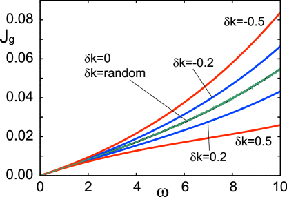
Figure 8: Stability of the driving. For the plot “$\delta k=\mbox{random}$”, we choose $\delta k(t)$ randomly at each time between $-1$ and $1$. It almost overlaps with the result at $\delta k=0$.

References

[1]
D. J. Thouless,
Quantization of particle transport,
Phys. Rev. B 27, 6083 (1983).
[2]
Q. Niu and D. J. Thouless,
Quantised adiabatic charge transport in the presence of substrate disorder and many-body interaction,
J. Phys. A 17, 2453 (1984).
[3]
M. V. Berry,
Quantal phase factors accompanying adiabatic changes,
Proc. R. Soc. London A 392, 45 (1984).
[4]
P. W. Brouwer,
Scattering approach to parametric pumping,
Phys. Rev. B 58, R10135 (1998).
[5]
J. M. R. Parrondo,
Reversible ratchets as Brownian particles in an adiabatically changing periodic potential,
Phys. Rev. E 57, 7297 (1998).
[6]
O. Usmani, E. Lutz, and M. Büttiker,
Noise-assisted classical adiabatic pumping in a symmetric periodic potential,
Phys. Rev. E 66, 021111 (2002).
[7]
R. D. Astumian,
Adiabatic Pumping Mechanism for Ion Motive ATPases,
Phys. Rev. Lett. 91, 118102 (2003).
[8]
R. D. Astumian,
Adiabatic operation of a molecular machine,
Proc. Natl. Acad. Sci. U.S.A. 104, 19715 (2007).
[9]
N. A. Sinitsyn and I. Nemenman,
The Berry phase and the pump flux in stochastic chemical kinetics,
Europhys. Lett. 77, 58001 (2007).
[10]
N. A. Sinitsyn and I. Nemenman,
Universal Geometric Theory of Mesoscopic Stochastic Pumps and Reversible Ratchets,
Phys. Rev. Lett. 99, 220408 (2007).
[11]
S. Rahav, J. Horowitz, and C. Jarzynski,
Directed Flow in Nonadiabatic Stochastic Pumps,
Phys. Rev. Lett. 101, 140602 (2008).
[12]
V. Y. Chernyak, J. R. Klein, and N. A. Sinitsyn,
Quantization and fractional quantization of currents in periodically driven stochastic systems. I. Average currents,
J. Chem. Phys. 136, 154107 (2012).
[13]
V. Y. Chernyak, J. R. Klein, and N. A. Sinitsyn,
Quantization and fractional quantization of currents in periodically driven stochastic systems. II. Full counting statistics,
J. Chem. Phys. 136, 154108 (2012).
[14]
F. Renzoni and T. Brandes,
Charge transport through quantum dots via time-varying tunnel coupling,
Phys. Rev. B 64, 245301 (2001).
[15]
T. Brandes and T. Vorrath,
Adiabatic transfer of electrons in coupled quantum dots,
Phys. Rev. B 66, 075341 (2002).
[16]
E. Cota, R. Aguado, and G. Platero,
ac-Driven Double Quantum Dots as Spin Pumps and Spin Filters,
Phys. Rev. Lett. 94, 107202 (2005).
[17]
T. Yuge, T. Sagawa, A. Sugita, and H. Hayakawa,
Geometrical pumping in quantum transport: Quantum master equation approach,
Phys. Rev. B 86, 235308 (2012).
[18]
T. Yuge, T. Sagawa, A. Sugita, and H. Hayakawa,
Geometrical excess entropy production in nonequilibrium quantum systems,
J. Stat. Phys. 153, 412 (2013).
[19]
S. Nakajima, M. Taguchi, T. Kubo, and Y. Tokura,
Interaction effect on adiabatic pump of charge and spin in quantum dot,
Phys. Rev. B 92, 195420 (2015).
[20]
S. Nakajima and Y. Tokura,
Excess entropy production in quantum system: Quantum master equation approach,
J. Stat. Phys. 169, 902 (2017).
[21]
H. Pothier, P. Lafarge, C. Urbina, D. Esteve, and M. H. Devoret,
Single-electron pump based on charging effects,
Europhys. Lett. 17, 249 (1992).
[22]
M. Switkes, C. M. Marcus, K. Campman, and A. C. Gossard,
An adiabatic quantum electron pump,
Science 283, 1905 (1999).
[23]
M. D. Blumenthal, B. Kaestner, L. Li, S. Giblin, T. J. B. M. Janssen, M. Pepper, D. Anderson, G. Jones, and D. A. Ritchie,
Gigahertz quantized charge pumping,
Nat. Phys. 3, 343 (2007).
[24]
B. Kaestner, V. Kashcheyevs, S. Amakawa, M. D. Blumenthal, L. Li, T. J. B. M. Janssen, G. Hein, K. Pierz, T. Weimann, U. Siegner, and H. W. Schumacher,
Single-parameter nonadiabatic quantized charge pumping,
Phys. Rev. B 77, 153301 (2008).
[25]
D. Xiao, M.-C. Chang, and Q. Niu,
Berry phase effects on electronic properties,
Rev. Mod. Phys. 82, 1959 (2010).
[26]
S. Nakajima, T. Tomita, S. Taie, T. Ichinose, H. Ozawa, L. Wang, M. Troyer, and Y. Takahashi,
Topological Thouless pumping of ultracold fermions,
Nat. Phys. 12, 296 (2016).
[27]
M. Lohse, C. Schweizer, O. Zilberberg, M. Aidelsburger, and I. Bloch,
A Thouless quantum pump with ultracold bosonic atoms in an optical superlattice,
Nat. Phys. 12, 350 (2016).
[28]
W. Ma, L. Zhou, Q. Zhang, M. Li, C. Cheng, J. Geng, X. Rong, F. Shi, J. Gong, and J. Du,
Experimental Observation of a Generalized Thouless Pump with a Single Spin,
Phys. Rev. Lett. 120, 120501 (2018).
[29]
L. S. Levitov and G. B. Lesovik,
Charge distribution in quantum shot noise,
JETP Lett. 58, 230 (1993).
[30]
L. S. Levitov, H.-W. Lee, and G. B. Lesovik,
Electron counting statistics and coherent states of electric current,
J. Math. Phys. (N.Y.) 37, 4845 (1996).
[31]
D. A. Bagrets and Yu. V. Nazarov,
Full counting statistics of charge transfer in Coulomb blockade systems,
Phys. Rev. B 67, 085316 (2003).
[32]
D. J. Evans, E. G. D. Cohen, and G. P. Morriss,
Probability of Second Law Violations in Shearing Steady States,
Phys. Rev. Lett. 71, 2401 (1993).
[33]
G. Gallavotti and E. G. D. Cohen,
Dynamical Ensembles in Nonequilibrium Statistical Mechanics,
Phys. Rev. Lett. 74, 2694 (1995).
[34]
K. Saito and Y. Utsumi,
Symmetry in full counting statistics, fluctuation theorem, and relations among nonlinear transport coefficients in the presence of a magnetic field,
Phys. Rev. B 78, 115429 (2008).
[35]
T. Sagawa and H. Hayakawa,
Geometrical expression of excess entropy production,
Phys. Rev. E 84, 051110 (2011).
[36]
Y. Aharonov and J. Anandan,
Phase Change During a Cyclic Quantum Evolution,
Phys. Rev. Lett. 58, 1593 (1987).
[37]
J. Samuel and R. Bhandari,
General Setting for Berry’s Phase,
Phys. Rev. Lett. 60, 2339 (1988).
[38]
A. Bohm, A. Mostafazadeh, H. Koizumi, Q. Niu, and J. Zwanziger,
The Geometric Phase in Quantum Systems (Springer, Berlin, 2003).
[39]
J. Ren, P. Hänggi, and B. Li,
Berry-Phase-Induced Heat Pumping and Its Impact on the Fluctuation Theorem,
Phys. Rev. Lett. 104, 170601 (2010).
[40]
K. L. Watanabe and H. Hayakawa,
Geometric fluctuation theorem for a spin-boson system,
Phys. Rev. E 96, 022118 (2017).
[41]
Y. Hino and H. Hayakawa,
Fluctuation relations for adiabatic quantum pumping,
arXiv:1908.10597.
[42]
J. Ohkubo,
The stochastic pump current and the non-adiabatic geometrical phase,
J. Stat. Mech. (2008) P02011.
[43]
J. Ohkubo,
Current and fluctuation in a two-state stochastic system under nonadiabatic periodic perturbation,
J. Chem. Phys. 129, 205102 (2008).
[44]
F. Cavaliere, M. Governale, and J. König,
Nonadiabatic Pumping Through Interacting Quantum Dots,
Phys. Rev. Lett. 103, 136801 (2009).
[45]
J. Ohkubo,
Noncyclic geometric phase in counting statistics and its role as an excess contribution,
J. Phys. A 46, 285001 (2013).
[46]
C. Uchiyama,
Nonadiabatic effect on the quantum heat flux control,
Phys. Rev. E 89, 052108 (2014).
[47]
K. L. Watanabe and H. Hayakawa,
Non-adiabatic effect in quantum pumping for a spin-boson system,
Prog. Theor. Exp. Phys. 2014, 113A01 (2014).
[48]
L. Privitera, A. Russomanno, R. Citro, and G. E. Santoro,
Nonadiabatic Breaking of Topological Pumping,
Phys. Rev. Lett. 120, 106601 (2018).
[49]
S. Kitamura, N. Nagaosa, and T. Morimoto,
Nonreciprocal Landau–Zener tunneling,
arXiv:1908.00819.
[50]
M. Demirplak and S. A. Rice,
Adiabatic population transfer with control fields,
J. Phys. Chem. A 107, 9937 (2003).
[51]
M. Demirplak and S. A. Rice,
Assisted adiabatic passage revisited,
J. Phys. Chem. B 109, 6838 (2005).
[52]
M. V. Berry,
Transitionless quantum driving,
J. Phys. A 42, 365303 (2009).
[53]
X. Chen, A. Ruschhaupt, S. Schmidt, A. del Campo, D. Guéry-Odelin,
and J. G. Muga,
Fast Optimal Frictionless Atom Cooling in Harmonic Traps: Shortcut to Adiabaticity,
Phys. Rev. Lett. 104, 063002 (2010).
[54]
E. Torrontegui, S. Ibáñez, S. Martínez-Garaot, M. Modugno,
A. del Campo, D. Guéry-Odelin, A. Ruschhaupt, X. Chen, and J. G. Muga,
Shortcuts to adiabaticity,
Adv. At. Mol. Opt. Phys. 62, 117 (2013).
[55]
D. Guéry-Odelin, A. Ruschhaupt, A. Kiely, E. Torrontegui, S. Martínez-Garaot, and J. G. Muga,
Shortcuts to adiabaticity: Concepts, methods, and applications,
Rev. Mod. Phys. 91, 045001 (2019).
[56]
K. Nishimura and K. Takahashi,
Counterdiabatic Hamiltonians for multistate Landau-Zener problem,
SciPost Phys. 5, 029 (2018).
[57]
W. Magnus,
On the exponential solution of differential equations for a linear operator,
Commun. Pure Appl. Math. 7, 649 (1954).
[58]
S. Blanes, F. Casas, J. Oteo, and J. Ros,
The Magnus expansion and some of its applications,
Phys. Rep. 470, 151 (2009).
[59]
S. Ibáñez, S. Martínez-Garaot, X. Chen, E. Torrontegui, and J. G. Muga,
Shortcuts to adiabaticity for non-Hermitian systems,
Phys. Rev. A 84, 023415 (2011).
[60]
Z. C. Tu,
Stochastic heat engine with the consideration of inertial effects and shortcuts to adiabaticity,
Phys. Rev. E 89, 052148 (2014).
[61]
K. Takahashi and M. Ohzeki,
Conflict between fastest relaxation of a Markov process and detailed balance condition,
Phys. Rev. E 93, 012129 (2016).
[62]
G. Li, H. T. Quan, and Z. C. Tu,
Shortcuts to isothermality and nonequilibrium work relations,
Phys. Rev. E 96, 012144 (2017).
[63]
S. Campbell and S. Deffner,
Trade-Off Between Speed and Cost in Shortcuts to Adiabaticity,
Phys. Rev. Lett. 118, 100601 (2017).
[64]
K. Funo, J.-N. Zhang, C. Chatou, K. Kim, M. Ueda, and A. del Campo,
Universal Work Fluctuations During Shortcuts to Adiabaticity
by Counterdiabatic Driving,
Phys. Rev. Lett. 118, 100602 (2017).
[65]
K. Takahashi,
How fast and robust is the quantum adiabatic passage?,
J. Phys. A 46, 315304 (2013).
[66]
K. Funo, N. Lambert, F. Nori, and C. Flindt,
Shortcuts to Adiabatic Pumping in Classical Stochastic Systems,
Phys. Rev. Lett. 124, 150603 (2020).