Phenomenology of the new light Higgs bosons in Gildener-Weinberg models

Abstract

Gildener-Weinberg (GW) models of electroweak symmetry breaking are especially interesting because the low mass and nearly Standard Model couplings of the $125\,{\rm GeV}$ Higgs boson, $H$, are protected by approximate scale symmetry. Another important but so far under-appreciated feature of these models is that a sum rule bounds the masses of the new charged and neutral Higgs bosons appearing in all these models to be below about $500\,{\rm GeV}$. Therefore, they are within reach of LHC data currently or soon to be in hand. Also so far unnoticed of these models, certain cubic and quartic Higgs scalar couplings vanish at the classical level. This is due to spontaneous breaking of the scale symmetry. These couplings become nonzero from explicit scale breaking in the Coleman-Weinberg loop expansion of the effective potential. In a two-Higgs doublet GW model, we calculate $\lambda_{HHH}\simeq 2(\lambda_{HHH})_{\rm SM}=64\,{\rm GeV}$. This corresponds to $\sigma(pp\to HH)\cong 15$–$20\,{\rm fb}$, its minimum value for $\sqrt{s}=13$–$14\,{\rm TeV}$ at the LHC. It will require at least the $27\,{\rm TeV}$ HE-LHC to observe this cross section. We also find $\lambda_{HHHH}\simeq 4(\lambda_{HHHH})_{\rm SM}=0.129$, whose observation in $pp\to HHH$ requires a $100\,{\rm TeV}$ collider. Because of the above-mentioned sum rule, these results apply to all GW models. In view of this unpromising forecast, we stress that LHC searches for the new relatively light Higgs bosons of GW models are by far the surest way to test them in this decade.

I. Synopsis

Section II of this paper reviews the Gildener-Weinberg (GW) mechanism for producing a model of a naturally light and aligned Higgs boson, $H$, in multi-Higgs-scalar models of electroweak symmetry breaking [1]. This is done in the context of a two-Higgs doublet model (2HDM) due to Lee and Pilaftsis [2]. The tree-level Higgs potential in GW models is scale-invariant, but that symmetry can be spontaneously broken, resulting in $H$ as a massless dilaton with exactly Standard Model (SM) couplings to gauge bosons and fermions. This scale symmetry is explicitly broken in one-loop order of the Coleman-Weinberg effective potential [3], resulting in $M_{H}^{2}>0$, but only small deviations from its exact SM couplings. An important corollary of the formula for $M_{H}^{2}$ is a sum rule for the masses of the additional Higgs scalars, generically ${\cal H}$. In any GW model of electroweak breaking in which the only weak bosons are $W^{\pm}$ and $Z^{0}$ and the only heavy fermion is the top quark, the sum rule in first-order loop-perturbation theory is [2, 4, 5]

$$\left(\sum_{{\cal H}}M_{{\cal H}}^{4}\right)^{1/4}=540\,{\rm GeV}.$$ (1)

In the GW-2HDM model, the additional Higgs bosons are a charged pair, $H^{\pm}$, and one $C\!P$-even and one $C\!P$-odd scalar, which we call $H_{2}$ and $A$. This sum rule has profound consequences for the phenomenology of GW models that this paper emphasizes. For example, in a search for these new Higgses, care must be taken in using the sum rule to estimate the light scalar’s mass when the other scalar masses are assumed to exceed 400–500 GeV.

In Sec. III we discuss features of the cubic and quartic Higgs boson self-couplings peculiar to GW models. As a consequence of unbroken scale invariance in the classical Higgs potential, certain of them vanish. These couplings do become nonzero once the scale symmetry is explicitly broken. We calculate the most important of these, finding that the experimentally most relevant ones, $\lambda_{HHH}$ and $\lambda_{HHHH}$, imply $\sigma(pp\to HH)$ and $\sigma(pp\to HHH)$ too small to detect at even the High-Luminosity (HL) LHC [6]. Again, because of the sum rule (1), this conclusion is true in all GW models of electroweak symmetry breaking, regardless of their Higgs sector.

This leads to Sec. IV where we refocus on direct searches at the LHC for the new light Higgs bosons of GW models. We briefly summarize these Higgses’ main search channels and the status of these searches. Substantial progress is in reach of data in hand or to be collected in the near future. There is nothing exotic about these searches; what is required for discovery or exclusion is greater sensitivity at relatively low masses.

II. The Two-Higgs Doublet Model

In 1976, E. Gildener and S. Weinberg (GW) proposed a scheme, based on broken scale symmetry, to generate a light Higgs boson in multi-scalar models of electroweak symmetry breaking. In essence, their motivation was to generalize the work of S. Coleman and E. Weinberg [3] to completely general electroweak models, with arbitrary gauge groups and representations of the fermions and scalars. What GW did not appreciate then — there was no reason for them to — was that their Higgs boson was also aligned [7]. That is, of all the scalars, its couplings to gauge bosons and fermions were exactly those of the single Higgs boson of the Standard Model (SM) [8]. Like the Higgs boson’s mass, its alignment is protected by the approximate scale symmetry [5].

GW assumed an electroweak Lagrangian whose Higgs potential $V_{0}$ has only quartic interactions. With no quadratic nor cubic Higgs couplings and, assuming that gauge boson and fermion masses arise entirely from their couplings to Higgs scalars, the GW theory is scale invariant at the classical level. This Lagrangian may, however, have a nontrivial extremum. If it does, it is along a ray in scalar-field space and it is a flat minimum if the quartic couplings satisfy certain positivity conditions. Thus, scale symmetry is spontaneously broken at tree level, and there is a massless (Goldstone) dilaton, $H$, which GW called the “scalon”. Higgs alignment is a simple consequence of the linear combination of fields composing $H$ having the same form as the Goldstone bosons $w^{\pm}$ and $z$ that become the longitudinal components of the $W^{\pm}$ and $Z$ bosons; see Eqs. (14) below.

Importantly, scale symmetry is explicitly broken by the first-order term $V_{1}$ in the Coleman-Weinberg loop expansion of the effective scalar potential [3]: $V_{0}+V_{1}$ can have a deeper minimum than the trivial one at zero fields. If it does, it occurs at a specific vacuum expectation value (VEV) $\langle H\rangle=v$, explicitly breaking scale invariance. Then $M_{H}$ and all other masses in the theory are proportional to $v$. The GW scheme is the only one we know in which the entire breaking of scale and electroweak symmetries is caused by the same electroweak operator, namely, $\langle H\rangle$. Hence, the dilaton decay constant $f=v$ [9], which we take to be $246\,{\rm GeV}$.

In 2012, Lee and Pilaftsis (LP) proposed a simple 2HDM model of the GW mechanism employing the Higgs doublets [2]:

$$\Phi_{i}=\frac{1}{\sqrt{2}}\left(\begin{array}[]{c}\sqrt{2}\phi_{i}^{+}\\ \rho_{i}+ia_{i}\end{array}\right),\quad i=1,2.$$ (2)

Here, $\rho_{i}$ and $a_{i}$ are neutral $C\!P$-even and odd fields. Their potential is

$$V_{0}(\Phi_{1},\Phi_{2}) = \lambda_{1}(\Phi_{1}^{\dagger}\Phi_{1})^{2}+\lambda_{2}(\Phi_{2}^{\dagger}\Phi_{2})^{2}+\lambda_{3}(\Phi_{1}^{\dagger}\Phi_{1})(\Phi_{2}^{\dagger}\Phi_{2})$$ (3)

$$+ \lambda_{4}(\Phi_{1}^{\dagger}\Phi_{2})(\Phi_{2}^{\dagger}\Phi_{1})+\textstyle{\frac{1}{2}}\lambda_{5}\left((\Phi_{1}^{\dagger}\Phi_{2})^{2}+(\Phi_{2}^{\dagger}\Phi_{1})^{2}\right).$$

All five quartic couplings are real so that $V_{0}$ is $C\!P$-invariant as well. This potential is consistent with a ${\cal Z}_{2}$ symmetry that prevents tree-level flavor-changing interactions among fermions, $\psi$, induced by neutral scalar exchange [10]:

$$\Phi_{1}\to-\Phi_{1},\,\,\Phi_{2}\to\Phi_{2},\quad\psi_{L}\to-\psi_{L},\,\,\psi_{uR}\to\psi_{uR},\,\,\psi_{dR}\to\psi_{dR}.$$ (4)

This is the usual type-I 2HDM [11], but with $\Phi_{1}$ and $\Phi_{2}$ interchanged; we refer henceforth to this version of the model as the GW-2HDM. This choice of Higgs couplings differs from LP’s choice of type-II [2]. It was made to remain consistent with limits from CMS [12] and ATLAS [13] on charged Higgs decay into $t\bar{b}$. The limits from these papers are consistent with $\tan\beta\mathrel{\hbox to0.0pt{\raise 2.20013pt\hbox{$<$}\hss}{\lower 2.20013pt\hbox{$\sim$}}}0.5$ for $M_{H^{\pm}}\mathrel{\hbox to0.0pt{\raise 2.20013pt\hbox{$<$}\hss}{\lower 2.20013pt\hbox{$\sim$}}}500\,{\rm GeV}$. This range of $\tan\beta$ also suppresses $gg\to A(H^{\prime})\to\bar{b}b,\,\bar{t}t$, where $A(H^{\prime})$ is a $C\!P$-odd (even) Higgs, relative to a heavy Higgs boson $H$ with SM couplings. See the discussion and references in Ref. [5].

The potential $V_{0}$ can have a flat minimum along the ray

$$\Phi_{1\beta}=\frac{1}{\sqrt{2}}\left(\begin{array}[]{c}0\\ \phi\,c_{\beta}\end{array}\right),\quad\Phi_{2\beta}=\frac{1}{\sqrt{2}}\left(\begin{array}[]{c}0\\ \phi\,s_{\beta}\end{array}\right).$$ (5)

Here $\phi>0$ is any real mass scale, $c_{\beta}=\cos\beta$ and $s_{\beta}=\sin\beta$. The nontrivial tree-level extremal conditions are (for $\beta\neq 0,\pi/2$):

$$\lambda_{1}c_{\beta}^{2}+\textstyle{\frac{1}{2}}\lambda_{345}s_{\beta}^{2}=0,\qquad\lambda_{2}s_{\beta}^{2}+\textstyle{\frac{1}{2}}\lambda_{345}c_{\beta}^{2}=0,$$ (6)

where $\lambda_{345}=\lambda_{3}+\lambda_{4}+\lambda_{5}$. Scale symmetry is spontaneously, but not yet explicitly, broken. Note that $V_{0\beta}=V_{0}(\Phi_{1\beta},\Phi_{2\beta})=0$, degenerate with the trivial vacuum. The squared “mass” matrices of the $C\!P$-odd, charged, and $C\!P$-even scalars are given by

$${\cal M}^{2}_{S}=-\lambda_{S}\phi^{2}\left(\begin{array}[]{cc}s_{\beta}^{2}&-s_{\beta}c_{\beta}\\ -s_{\beta}c_{\beta}&c_{\beta}^{2}\end{array}\right),\\$$ (7)

where the subscript $S=H_{0^{-}}$, $H^{\pm}$, and $H_{0^{+}}$ In terms of the quartic couplings in the Higgs potential, they are $\lambda_{H_{0^{-}}}=\lambda_{5}$; $\lambda_{H^{\pm}}=\textstyle{\frac{1}{2}}(\lambda_{4}+\lambda_{5})=\textstyle{\frac{1}{2}}\lambda_{45}$; and $\lambda_{H_{0^{+}}}=\lambda_{345}$. All $\lambda_{S}$ are negative to ensure non-negative eigenvalues of the matrices. The respective eigenvectors and eigenvalues are:

$$\left(\begin{array}[]{c}z\\ A\end{array}\right) = \left(\begin{array}[]{cc}c_{\beta}&s_{\beta}\\ -s_{\beta}&c_{\beta}\end{array}\right)\left(\begin{array}[]{c}a_{1}\\ a_{2}\end{array}\right),\quad M_{z}^{2}=0,\,\,\,M_{A}^{2}=-\lambda_{5}\phi^{2};$$ (14)

$$\left(\begin{array}[]{c}w^{\pm}\\ H^{\pm}\end{array}\right) = \left(\begin{array}[]{cc}c_{\beta}&s_{\beta}\\ -s_{\beta}&c_{\beta}\end{array}\right)\left(\begin{array}[]{c}\phi_{1}^{\pm}\\ \phi_{2}^{\pm}\end{array}\right),\quad M_{w^{\pm}}^{2}=0,\,\,\,M_{H^{\pm}}^{2}=-\textstyle{\frac{1}{2}}\lambda_{45}\phi^{2};$$ (21)

$$\left(\begin{array}[]{c}H\\ H^{\prime}\end{array}\right) = \left(\begin{array}[]{cc}c_{\beta}&s_{\beta}\\ -s_{\beta}&c_{\beta}\end{array}\right)\left(\begin{array}[]{c}\rho_{1}\\ \rho_{2}\end{array}\right),\quad M_{H}^{2}=0,\,\,\,M^{2}_{H^{\prime}}=-\lambda_{345}\phi^{2}.$$ (28)

The one-loop effective potential, presented in Ref. [2], is given by

$$V_{1} = \frac{1}{64\pi^{2}}\biggl{[}6M_{W}^{4}\left(-\frac{5}{6}+\ln\frac{M_{W}^{2}}{\Lambda_{\rm GW}^{2}}\right)+3M_{Z}^{4}\left(-\frac{5}{6}+\ln\frac{M_{Z}^{2}}{\Lambda_{\rm GW}^{2}}\right)$$ (29)

$$\quad+M_{H^{\prime}}^{4}\left(-\frac{3}{2}+\ln\frac{M_{H^{\prime}}^{2}}{\Lambda_{\rm GW}^{2}}\right)+M_{A}^{4}\left(-\frac{3}{2}+\ln\frac{M_{A}^{2}}{\Lambda_{\rm GW}^{2}}\right)$$

$$\quad+2M_{H^{\pm}}^{4}\left(-\frac{3}{2}+\ln\frac{M_{H^{\pm}}^{2}}{\Lambda_{\rm GW}^{2}}\right)-12m_{t}^{4}\left(-1+\ln\frac{m_{t}^{2}}{\Lambda_{\rm GW}^{2}}\right)\biggr{]},$$

where $\Lambda_{GW}$ is the GW renormalization scale (related to the Higgs VEV $v$ by Eq. (40,41) in LP). The background field-dependent masses in $V_{1}$ are

$$M_{W}^{2} = \textstyle{\frac{1}{2}}g^{2}\left(\Phi_{1}^{\dagger}\Phi_{1}+\Phi_{2}^{\dagger}\Phi_{2}\right),$$

$$M_{Z}^{2} = \textstyle{\frac{1}{2}}(g^{2}+g^{\prime\,2})\left(\Phi_{1}^{\dagger}\Phi_{1}+\Phi_{2}^{\dagger}\Phi_{2}\right),$$

$$M_{A}^{2} = -2\lambda_{5}\left(\Phi_{1}^{\dagger}\Phi_{1}+\Phi_{2}^{\dagger}\Phi_{2}\right),$$

$$M_{H^{\pm}}^{2} = -\lambda_{45}\left(\Phi_{1}^{\dagger}\Phi_{1}+\Phi_{2}^{\dagger}\Phi_{2}\right),$$

$$M_{H^{\prime}}^{2} = -2\lambda_{345}\left(\Phi_{1}^{\dagger}\Phi_{1}+\Phi_{2}^{\dagger}\Phi_{2}\right),$$

$$m_{t}^{2} = \Gamma_{t}^{2}\,\Phi_{1}^{\dagger}\Phi_{1},$$ (30)

where $g,g^{\prime}$ are the electroweak $SU(2)$ and $U(1)$ gauge couplings and $\Gamma_{t}=\sqrt{2}m_{t}/v_{1}=\sqrt{2}m_{t}/v\cos\beta$ is the Higgs-Yukawa coupling of the top quark. In Eqs. (II. The Two-Higgs Doublet Model), the $C\!P$-even part of $\Phi_{i}$ is the shifted field $v_{i}+\rho_{i}$.

The nontrivial extremal conditions for $V_{0}+V_{1}$ are [2]

$$\left.\frac{\partial(V_{0}+V_{1})}{\partial\rho_{1}}\right|_{\langle\,\rangle} \propto \lambda_{1}c_{\beta}^{2}+\textstyle{\frac{1}{2}}\lambda_{345}s_{\beta}^{2}+\Delta\widehat{t}_{1}/64\pi^{2}=0,$$

$$\left.\frac{\partial(V_{0}+V_{1})}{\partial\rho_{2}}\right|_{\langle\,\rangle} \propto \lambda_{2}s_{\beta}^{2}+\textstyle{\frac{1}{2}}\lambda_{345}c_{\beta}^{2}+\Delta\widehat{t}_{2}/64\pi^{2}=0,$$ (31)

where $\langle\,\rangle$ means that the derivatives of $V_{0}+V_{1}$ are evaluated at the vacuum expectation values of the fields, and

$$\Delta\widehat{t}_{i} = \frac{4}{v^{4}}\biggl{[}2M_{W}^{4}\left(3\ln{\frac{M_{W}^{2}}{\Lambda_{\rm GW}^{2}}}-1\right)+M_{Z}^{4}\left(3\ln{\frac{M_{Z}^{2}}{\Lambda_{\rm GW}^{2}}}-1\right)+M_{H^{\prime}}^{4}\left(\ln{\frac{M_{H^{\prime}}^{2}}{\Lambda_{\rm GW}^{2}}}-1\right)$$ (32)

$$+M_{A}^{4}\left(\ln{\frac{M_{A}^{2}}{\Lambda_{\rm GW}^{2}}}-1\right)+2M_{H^{\pm}}^{4}\left(\ln{\frac{M_{H^{\pm}}^{2}}{\Lambda_{\rm GW}^{2}}}-1\right)-12m_{t}^{4}\left(\ln{\frac{m_{t}^{2}}{\Lambda_{\rm GW}^{2}}}-\frac{1}{2}\right)\delta_{i1}\biggr{]}_{\langle\,\rangle}.\hskip 28.45274pt$$

For nontrivial extrema with $\beta\neq 0,\,\pi/2$, these conditions lead to a deeper minimum than the zeroth-order ones, $(V_{0}+V_{1})_{\rm min}<V_{0\beta}=V_{0}(0)+V_{1}(0)=0$. This minimum occurs at a particular value $v$ of the scale $\phi$ which, as we’ve said, is identified as the electroweak breaking scale,  $v=246\,{\rm GeV}$. The VEVs of $\Phi_{1}$ and $\Phi_{2}$ are $v_{1}=v\cos\beta$ and $v_{2}=v\sin\beta$, with $\tan\beta=v_{2}/v_{1}$ as usual in 2HDM.

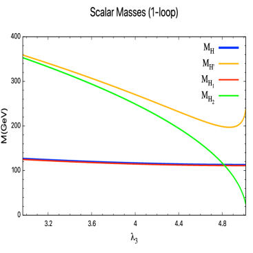
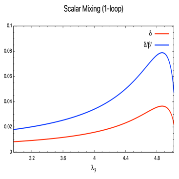
Figure 1: Left: The $C\!P$-even Higgs one-loop mass eigenvalues $M_{H_{1}}$ and $M_{H_{2}}$, the tree-level mass $M_{H^{\prime}}=\sqrt{-\lambda_{345}}\,v$ and the one-loop mass $M_{H}$ from Eq. (34) as functions of $\lambda_{3}=(2M_{H^{\pm}}^{2}-M_{H^{\prime}}^{2})/v^{2}$. Here, $\tan\beta=0.50$ and $M_{H^{\pm}}=M_{A}=390\,{\rm GeV}$ corresponding to $\lambda_{4}=\lambda_{5}=-2.513$. The input $H\cong H_{1}$ mass is $M_{H}=125.0\,{\rm GeV}$, the corresponding initial $M_{H^{\prime}}=353\,{\rm GeV}$ and $\lambda_{3}=2.966$. $M_{H^{\prime}}$ vanishes at $\lambda_{3}=2M^{2}_{H^{\pm}}/v^{2}=5.027$. Right: The angle $\delta=\beta-\beta^{\prime}$ measuring the deviation from perfect alignment of $H_{1}$ and the ratio $\delta/\beta$ for $\beta=0.4637$. The procedure used in creating these figures is spelled out in the Appendix of Ref. [5]

.

The $C\!P$-odd and charged Higgs bosons’ masses receive no contribution from $V_{1}$ and, so, they are given by Eqs. (14) with $\phi=v$. The $C\!P$-even masses, however, receive important corrections from $V_{1}$. The eigenvectors $H_{1}$ and $H_{2}$ are

$$H_{1} = c_{\delta}H-s_{\delta}H^{\prime}=c_{\beta^{\prime}}\rho_{1}+s_{\beta^{\prime}}\rho_{2},$$

$$H_{2} = s_{\delta}H+c_{\delta}H^{\prime}=-s_{\beta^{\prime}}\rho_{1}+c_{\beta^{\prime}}\rho_{2},$$ (33)

where $\beta^{\prime}=\beta-\delta$, $c_{\beta^{\prime}}=\cos\beta^{\prime}$, etc. The angle $\delta$ measures the departure of the Higgs boson $H_{1}$ from perfect alignment, and it should be small. Furthermore, the accuracy of first-order perturbation theory requires $|\delta/\beta|\ll 1$. Both these criteria are met in calculations with a wide range of input parameters; they are illustrated in Fig. 1. From now on we refer interchangeably to the 125 GeV Higgs boson as $H_{1}$ or $H$, as clarity requires. Its mass is given by [1],[2],[5]

$$M_{H_{1}}^{2}\cong M_{H}^{2}=\frac{1}{8\pi^{2}v^{2}}\left(6M_{W}^{4}+3M_{Z}^{4}+M_{H^{\prime}}^{4}+M_{A}^{4}+2M_{H^{\pm}}^{4}-12m_{t}^{4}\right).$$ (34)

In accord with first-order perturbation theory, all the masses on the right side of this formula are obtained from zeroth-order perturbation theory, i.e., from $V_{0}$ plus gauge and Yukawa interactions, with $\phi=v$. As we see in Fig. 1, the Higgs masses $M_{H}$ and $M_{H_{1}}$ derived from Eq. (34) and from diagonalizing the one-loop mass matrix ${\cal M}_{H_{0^{+}}}$ respectively, are extremely close, as they should be.

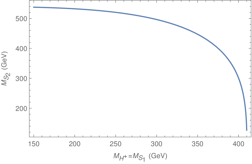
Figure 2: The mass of the neutral Higgs $S_{2}=H^{\prime}$ $(S_{2}=M_{A})$ as a function of the common mass of $H^{\pm}$ and the other neutral Higgs, $S_{1}=A$ $(S_{1}=H^{\prime})$, from Eqs.(34,35) with $M_{H}=125\,{\rm GeV}$. Note the considerable sensitivity of $M_{S_{2}}$ to small changes in $M_{H^{+}}=M_{S_{1}}$ when it is large. From Ref. [5]

This formula can be used in two related ways. First, assuming that there are no other heavy fermions and weak bosons, it implies a sum rule on all the new scalar masses in this GW-2HDM [2, 4, 5]:

$$\left(M_{H^{\prime}}^{4}+M_{A}^{4}+2M_{H^{\pm}}^{4}\right)^{1/4}=540\,{\rm GeV}.$$ (35)

The sum rule is illustrated in Fig. 2 for $M_{H}\cong M_{H_{1}}=125\,{{\rm GeV}}$ and $M_{H^{\pm}}=M_{S_{1}}$, where $M_{S_{1}}=M_{A}$ or $M_{H^{\prime}}$; the mass of the other neutral scalar, $M_{S_{2}}$, is plotted against $M_{H^{\pm}}=M_{S_{1}}$. The smallness of $\delta$ in Fig. 1 and the magnitude of Higgs couplings we obtain in Sec. III give us confidence that the one-loop approximation (34) is reliable. Still, we would not be surprised if higher-order corrections change the right side of Eq. (35) by ${\cal O}(100\,{\rm GeV})$. The important point is that the sum rule tells us that new Higgs bosons should be found at surprisingly low masses. To repeat: this sum rule holds in any GW model of electroweak breaking in which the only weak bosons are $W$ and $Z$ and the only heavy fermion is the top quark. Thus, the larger the Higgs sector, the lighter will be the masses of at least some of the new Higgs bosons expected in a GW model.

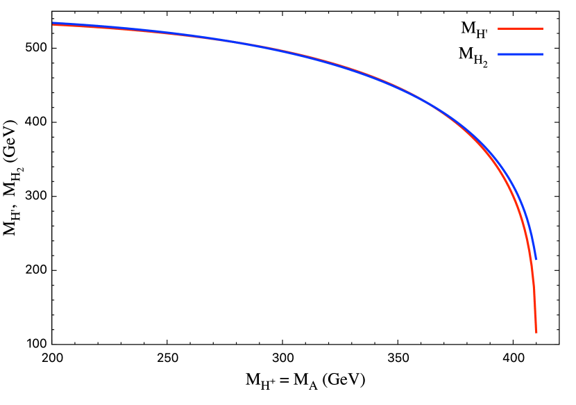
Figure 3: The tree-approximation mass $M_{H^{\prime}}$ of the $C\!P$-even Higgs calculated from the sum rule (35) and the larger eigenvalue $M_{H_{2}}$ of the one-loop corrected $C\!P$-even mass matrix ${\cal M}_{H_{0^{+}}}$. Both are calculated as a function of $M_{H^{\pm}}=M_{A}$. $M_{H^{\prime}}$ starts to dive to zero at $M_{H^{\pm}}\cong 370\,{\rm GeV}$ and becomes zero at $M_{H^{\pm}}\cong 410.22\,{\rm GeV}$.

Second, as an instructive example in the present model, we assume that $M_{H^{\pm}}=M_{A}$ and imagine searching for $H_{2}\simeq H^{\prime}$. (The assumption $M_{H^{\pm}}=M_{A}$ is motivated by the fact that it makes the contribution to the $T$-parameter from the scalars vanish identically [14, 15].) Due to the sum-rule constraint in Eq. (35), the mass of $M_{H^{\prime}}$ is very sensitive to small changes in $M_{H^{\pm}}$ when it is large. Fig. 2 suggests we can use the sum rule until $M_{H^{\prime}}$ starts to dive to zero. To be quantitative about this, Fig. 3 shows $M_{H^{\prime}}$ and $M_{H_{2}}$ as a function of $M_{H^{\pm}}=M_{A}$ over the range allowed by the sum rule. The two masses are very nearly equal up to $M_{H^{\pm}}=370\,{\rm GeV}$. At that mass, $M_{H^{\prime}}\cong M_{H_{2}}=412\,{\rm GeV}$ and, beyond it, $M_{H^{\prime}}$ starts its dive. The most sensible thing to do, in our opinion, is to use the large $C\!P$-even mass eigenvalue, $M_{H_{2}}$, over the entire considered range of $M_{H^{\pm}}=M_{A}$.

We will do this for our estimates of the scalars’ production cross sections and decay branching ratios in Sec. IV. We recommend this approach for searches by ATLAS and CMS. For example, in a search involving the three GW Higgs bosons (say, $pp\to A\to ZH_{2}$ and $pp\to H^{\pm}\to W^{\pm}H_{2}$, with $H_{2}\to b\bar{b}$), one could use ellipsoidal search regions in ($M_{H^{\pm}},M_{A},M_{H_{2}}$)-space roughly consistent with $M_{H^{\pm}}=M_{A}$ and the sum rule, and calculate the model’s predicted $\sigma\cdot{\rm BR}$’s accordingly. Therefore, as with $H$ and $H_{1}$, we refer henceforth to the heavier $C\!P$-even scalar as $H^{\prime}$ or $H_{2}$, as clarity or the situation requires.

III. Triple and Quartic Higgs Couplings

In GW models of electroweak symmetry breaking, the tree-level triple-scalar couplings involving two or three of the Goldstone bosons $H,z,w^{\pm}$ vanish, as do the quartic couplings involving three or four of them. This is unlike any other multi-Higgs model. The reason for this, of course, must be scale invariance of the tree-level Lagrangian, in particular, that the potential $V_{0}$ contains only quartic couplings. But how does it work? We show how in this section. Then we calculate at one-loop order the triple-scalar couplings involving at least one $H\cong H_{1}$ and the quartic coupling $\lambda_{H_{1}H_{1}H_{1}H_{1}}$.

The way to see simply why certain scalar couplings vanish is to write $V_{0}$ in the “aligned basis”:

$$\Phi=\Phi_{1}c_{\beta}+\Phi_{2}s_{\beta},\quad\Phi^{\prime}=-\Phi_{1}s_{\beta}+\Phi_{2}c_{\beta}.$$ (36)

On the ray Eq. (5) on which $V_{0}$ has nontrivial extrema, these fields are

$$\Phi_{\beta}=\frac{1}{\sqrt{2}}\left(\begin{array}[]{c}0\\ \phi\end{array}\right),\quad\Phi^{\prime}_{\beta}=\frac{1}{\sqrt{2}}\left(\begin{array}[]{c}0\\ 0\end{array}\right),$$ (37)

where $\phi\in(0,\infty)$ is a constant mass scale. Then, in terms of the tree-level mass-eigenstate scalars, the fields $\Phi$, $\Phi^{\prime}$ are

$$\Phi=\frac{1}{\sqrt{2}}\left(\begin{array}[]{c}\sqrt{2}w^{+}\\ \phi+H+iz\end{array}\right),\quad\Phi^{\prime}=\frac{1}{\sqrt{2}}\left(\begin{array}[]{c}\sqrt{2}H^{+}\\ H^{\prime}+iA\end{array}\right).$$ (38)

Rewritten in terms of quartic polynomials in $\Phi$ and $\Phi^{\prime}$, Eq. (3) becomes (with $\lambda_{345}=\lambda_{3}+\lambda_{4}+\lambda_{5}$, etc.)

$$V_{0} = \left[\lambda_{1}c_{\beta}^{4}+\lambda_{2}s_{\beta}^{4}+\lambda_{345}s_{\beta}^{2}c_{\beta}^{2}\right]\left(\Phi^{\dagger}\Phi\right)^{2}$$ (39)

$$+\left[(2\lambda_{2}s_{\beta}^{2}+\lambda_{345}c_{\beta}^{2})-(2\lambda_{1}c_{\beta}^{2}+\lambda_{345}s_{\beta}^{2})\right]s_{\beta}c_{\beta}\left(\Phi^{\dagger}\Phi\right)\left(\Phi^{\dagger}\Phi^{\prime}+\Phi^{\prime\,\dagger}\Phi\right)$$

$$+\left[2(\lambda_{1}+\lambda_{2}-\lambda_{345})s_{\beta}^{2}c_{\beta}^{2}+\lambda_{3}\right]\left(\Phi^{\dagger}\Phi\right)\left(\Phi^{\prime\,\dagger}\Phi^{\prime}\right)$$

$$+\left[2(\lambda_{1}+\lambda_{2}-\lambda_{345})s_{\beta}^{2}c_{\beta}^{2}+\lambda_{4}\right]\left(\Phi^{\dagger}\Phi^{\prime}\right)\left(\Phi^{\prime\,\dagger}\Phi\right)$$

$$+\textstyle{\frac{1}{2}}\left[2(\lambda_{1}+\lambda_{2}-\lambda_{345})s_{\beta}^{2}c_{\beta}^{2}+\lambda_{5}\right]\left[\left(\Phi^{\dagger}\Phi^{\prime}\right)^{2}+\left(\Phi^{\prime\,\dagger}\Phi\right)^{2}\right]$$

$$+\left[(2\lambda_{2}c_{\beta}^{2}+\lambda_{345}s_{\beta}^{2})-(2\lambda_{1}s_{\beta}^{2}+\lambda_{345}c_{\beta}^{2})\right]s_{\beta}c_{\beta}\left(\Phi^{\prime\,\dagger}\Phi^{\prime}\right)\left(\Phi^{\dagger}\Phi^{\prime}+\Phi^{\prime\,\dagger}\Phi\right)$$

$$+\left[\lambda_{1}s_{\beta}^{4}+\lambda_{2}c_{\beta}^{4}+\lambda_{345}s_{\beta}^{2}c_{\beta}^{2}\right]\left(\Phi^{\prime\,\dagger}\Phi^{\prime}\right)^{2}.$$

By virtue of its scale invariance, $V_{0}$ is a homogeneous polynomial of degree four:

$$V_{0} = {\frac{1}{4}}\sum_{i=1}^{2}\left[\Phi_{i}^{\dagger}\frac{\partial V_{0}}{\partial\Phi_{i}^{\dagger}}+\frac{\partial V_{0}}{\partial\Phi_{i}}\Phi_{i}\right]$$ (40)

$$= {\frac{1}{4}}\left[\Phi^{\dagger}\frac{\partial V_{0}}{\partial\Phi^{\dagger}}+\frac{\partial V_{0}}{\partial\Phi}\Phi+\Phi^{\prime\,\dagger}\frac{\partial V_{0}}{\partial\Phi^{\prime\,\dagger}}+\frac{\partial V_{0}}{\partial\Phi^{\prime}}\Phi^{\prime}\right].$$

Thus, $V_{0}$ vanishes at any extremum, in particular for $\Phi_{\beta}=(0,\phi)/\sqrt{2}$ and $\Phi^{\prime}_{\beta}=(0,0)$, the flat direction associated with spontaneous scale symmetry breaking. We know that the conditions for the nontrivial extrema of $V_{0}$ are those in Eq. (6). It follows that the coefficients of $(\Phi^{\dagger}\Phi)^{2}$ and $(\Phi^{\dagger}\Phi)(\Phi^{\dagger}\Phi^{\prime}+\Phi^{{}^{\prime}\,\dagger}\Phi)$ terms in $V_{0}$ vanish. It is easy to see why these coefficients, $C_{1}$ and $C_{2}$, had to vanish. On the ray $\Phi_{\beta},\Phi^{\prime}_{\beta}$,

$$\left.\frac{\partial V_{0}}{\partial\Phi}\right|_{\Phi_{\beta},\Phi^{\prime}_{\beta}} = 2C_{1}\Phi^{\dagger}_{\beta}\left(\Phi^{\dagger}_{\beta}\Phi_{\beta}\right),$$ (41)

$$\left.\frac{\partial V_{0}}{\partial\Phi^{\prime}}\right|_{\Phi_{\beta},\Phi^{\prime}_{\beta}} = C_{2}\left(\Phi^{\dagger}_{\beta}\Phi_{\beta}\right)\Phi^{\dagger}_{\beta}.$$ (42)

Neither operator vanishes, hence their coefficients must. This would not have happened had $V_{0}$ also contained polynomials of degree less than four. That is, spontaneously broken scale invariance is the reason for the vanishing Goldstone boson couplings at tree level. And it is obvious that this analysis using homogeneous polynomials of fourth degree generalizes to any GW model of the electroweak interactions.

Using the tree-level extremal conditions, the nonzero coefficients in $V_{0}$ are simplified by using

$$2(\lambda_{1}+\lambda_{2}-\lambda_{345})s_{\beta}^{2}c_{\beta}^{2}=-\lambda_{345},$$ (43)

$$\left[(2\lambda_{2}c_{\beta}^{2}+\lambda_{345}s_{\beta}^{2})-(2\lambda_{1}s_{\beta}^{2}+\lambda_{345}c_{\beta}^{2})\right]s_{\beta}c_{\beta}=-2\lambda_{345}\cot 2\beta,$$ (44)

$$\lambda_{1}s_{\beta}^{4}+\lambda_{2}c_{\beta}^{4}+\lambda_{345}s_{\beta}^{2}c_{\beta}^{2}=-2\lambda_{345}\cot^{2}2\beta.$$ (45)

Then,

$$V_{0} = -\lambda_{45}\left(\Phi^{\dagger}\Phi\right)\left(\Phi^{\prime\,\dagger}\Phi^{\prime}\right)-\lambda_{35}\left(\Phi^{\dagger}\Phi^{\prime}\right)\left(\Phi^{\prime\,\dagger}\Phi\right)-\textstyle{\frac{1}{2}}\lambda_{34}\left[\left(\Phi^{\dagger}\Phi^{\prime}\right)^{2}+\left(\Phi^{\prime\,\dagger}\Phi\right)^{2}\right]$$ (46)

$$-2\lambda_{345}\cot 2\beta\left(\Phi^{\prime\,\dagger}\Phi^{\prime}\right)\left(\Phi^{\dagger}\Phi^{\prime}+\Phi^{\prime\,\dagger}\Phi\right)-2\lambda_{345}\cot^{2}2\beta\left(\Phi^{\prime\,\dagger}\Phi^{\prime}\right)^{2}.$$

From this, the masses in Eq. (7) may be read off from the first three terms.

With foreknowledge, we now put $\phi=v=246\,{\rm GeV}$. Then the nonzero cubic terms terms in the tree-level potential, written in terms of mass eigenstate scalars of $V_{0}$, are:

$$V_{0}({\rm cubic}) = -\textstyle{\frac{1}{2}}\lambda_{45}\,vH\left[(H^{\prime})^{2}+A^{2}+2H^{+}H^{-}\right]$$ (47)

$$-\textstyle{\frac{1}{2}}\lambda_{35}\,v\bigl{[}H^{\prime}(HH^{\prime}+zA+w^{+}H^{-}+H^{+}w^{-})$$

$$\qquad+A(HA-zH^{\prime})+iA(w^{+}H^{-}-H^{+}w^{-})\bigr{]}$$

$$-\textstyle{\frac{1}{2}}\lambda_{34}\,v\bigl{[}H^{\prime}(HH^{\prime}+zA+w^{+}H^{-}+H^{+}w^{-})$$

$$\qquad-A(HA-zH^{\prime})-iA(w^{+}H^{-}-H^{+}w^{-})\bigr{]}$$

$$-\lambda_{345}\cot 2\beta\,vH^{\prime}\left[(H^{\prime})^{2}+A^{2}+2H^{+}H^{-}\right].$$

The quartic terms are:

$$V_{0}({\rm quartic}) = -\textstyle{\frac{1}{4}}\lambda_{45}(H^{2}+z^{2}+2w^{+}w^{-})\left[(H^{\prime})^{2}+A^{2}+2H^{+}H^{-}\right]$$ (48)

$$-\textstyle{\frac{1}{4}}\lambda_{35}\bigl{[}(HH^{\prime}+zA+2w^{+}H^{-})(HH^{\prime}+zA+2H^{+}w^{-})$$

$$\qquad+(HA-zH^{\prime})^{2}+2i(HA-zH^{\prime})(w^{+}H^{-}-H^{+}w^{-})\bigr{]}$$

$$-\textstyle{\frac{1}{4}}\lambda_{34}\bigl{[}\textstyle{\frac{1}{2}}(HH^{\prime}+zA+2w^{+}H^{-})^{2}+\textstyle{\frac{1}{2}}(HH^{\prime}+zA+2H^{+}w^{-})^{2}$$

$$\qquad-(HA-zH^{\prime})^{2}-2i(HA-zH^{\prime})(w^{+}H^{-}-H^{+}w^{-})\bigr{]}$$

$$-\lambda_{345}\cot 2\beta\left[(H^{\prime})^{2}+A^{2}+2H^{+}H^{-}\right]\left[HH^{\prime}+zA+w^{+}H^{-}+H^{+}w^{-}\right]$$

$$-\textstyle{\frac{1}{2}}\lambda_{345}\cot^{2}2\beta\left[(H^{\prime})^{2}+A^{2}+2H^{+}H^{-}\right]^{2}.$$

Recall from Eq. (7) that $-\lambda_{345}=M_{H^{\prime}}^{2}/v^{2}$, $-\lambda_{45}=2M_{H^{\pm}}^{2}/v^{2}$ and $-\lambda_{5}=M_{A}^{2}/v^{2}$.

We turn to the one-loop corrections, focusing on the triple-scalar couplings involving the $125\,{\rm GeV}$ Higgs boson, $H\cong H_{1}$, and the quartic coupling $\lambda_{H_{1}H_{1}H_{1}H_{1}}$. For brevity, we include only those cubic couplings of $H_{1}$ with itself and with $H_{2}$. The $H_{1}AA$ and $H_{1}H^{+}H^{-}$ couplings are similar to $H_{1}H_{2}H_{2}$, as may be inferred from the tree-level cubics in Eq. (47) and Table 1 below. There are two types of one-loop corrections: (i) those to $V_{0}$ obtained by writing the zeroth-order $C\!P$-even fields in terms of $H_{1}$ and $H_{2}$, Eqs. (II. The Two-Higgs Doublet Model), and by using the one-loop extremal conditions, Eqs. (II. The Two-Higgs Doublet Model); (ii) those obtained from $V_{1}$ in Eq. (29) by isolating the coefficients of $H^{3}$, $H^{2}H^{\prime}$, etc.

(i) With $\rho_{i}$ shifted by $v_{i}$, the cubic $C\!P$-even terms in $V_{0}$ are:

$$V_{0}({\rm cubic}) = \lambda_{1}v_{1}\rho_{1}^{3}+\lambda_{2}v_{2}\rho_{2}^{3}+\textstyle{\frac{1}{2}}\lambda_{345}\left(v_{1}\rho_{1}\rho_{2}^{2}+v_{2}\rho_{2}\rho_{1}^{2}\right)$$ (49)

$$= -\lambda_{345}v\left(H(H^{\prime})^{2}+(H^{\prime})^{3}\cot 2\beta\right)-\frac{\Delta\widehat{t}_{1}}{64\pi^{2}c_{\beta}^{2}}\left[vc_{\beta}\left(Hc_{\beta}-H^{\prime}s_{\beta}\right)^{3}\right]$$

$$-\frac{\Delta\widehat{t}_{2}}{64\pi^{2}s_{\beta}^{2}}\left[vs_{\beta}\left(Hs_{\beta}+H^{\prime}c_{\beta}\right)^{3}\right].$$

Our convention for the triple and quartic couplings of $H_{1}$, for example, is that they are the coefficients of $H_{1}^{3}$ and $H_{1}^{4}$ in these two types of corrections. Then, the corrections to the triple-Higgs couplings from $V_{0}$ are:

$$\lambda^{(0)}_{H_{1}H_{1}H_{1}} = -\lambda_{345}\,v\,s_{\delta}^{2}(c_{\delta}-s_{\delta}\cot 2\beta)-\frac{(\Delta\widehat{t}_{1}c_{\beta}^{2}+\Delta\widehat{t}_{2}s_{\beta}^{2})\,v}{64\pi^{2}},$$ (50)

$$\lambda^{(0)}_{H_{1}H_{1}H_{2}} = +\lambda_{345\,}v\,s_{\delta}(2c_{\delta}^{2}-3s_{\delta}c_{\delta}\cot 2\beta-s_{\delta}^{2})+\frac{3(\Delta\widehat{t}_{1}-\Delta\widehat{t}_{2})\,vs_{\beta}c_{\beta}}{64\pi^{2}},\qquad$$ (51)

$$\lambda^{(0)}_{H_{1}H_{2}H_{2}} = -\lambda_{345}\,v\,c_{\delta}(c_{\delta}^{2}-3c_{\delta}s_{\delta}\cot 2\beta-2s_{\delta}^{2})-\frac{3(\Delta\widehat{t}_{1}s_{\beta}^{2}+\Delta\widehat{t}_{2}c_{\beta}^{2})\,v}{64\pi^{2}}.$$ (52)

(ii) To calculate the contributions to the triple-Higgs couplings from $V_{1}$, it is appropriate that we use the zeroth-order fields $H$ and $H^{\prime}$. Then,

$$\lambda^{(1)}_{H_{1}H_{1}H_{1}} = \left.\frac{1}{6}\,\frac{\partial^{3}V_{1}}{\partial H^{3}}\right|_{\langle\,\rangle},$$ (53)

$$\lambda^{(1)}_{H_{1}H_{1}H_{2}} = \left.\frac{1}{2}\,\frac{\partial^{3}V_{1}}{\partial H^{2}\,\partial H^{\prime}}\right|_{\langle\,\rangle},$$ (54)

$$\lambda^{(1)}_{H_{1}H_{2}H_{2}} = \left.\frac{1}{2}\,\frac{\partial^{3}V_{1}}{\partial H\,(\partial H^{\prime})^{2}}\right|_{\langle\,\rangle},$$ (55)

where, again, $\langle\,\rangle$ means that the derivatives are evaluated at the vacuum expectation values of the fields. Write $V_{1}$ as

$$V_{1}=\frac{1}{64\pi^{2}}\sum_{X}\alpha_{X}M_{X}^{4}\left(\beta_{X}+\ln(M_{X}^{2}/\Lambda_{\rm GW}^{2})\right),$$ (56)

where $M_{X}^{2}=g_{X}^{2}(\Phi_{1}^{\dagger}\Phi_{1}+\Phi_{2}^{\dagger}\Phi_{2})$, except that $m_{t}^{2}=\Gamma_{t}^{2}\,\Phi_{1}^{\dagger}\Phi_{1}$ with $\Gamma_{t}=\sqrt{2}m_{t}/v\cos\beta$. This $m_{t}^{2}$ affects $\lambda^{(1)}_{H_{1}H_{1}H_{2}}$ and $\lambda^{(1)}_{H_{1}H_{2}H_{2}}$. The constants $\alpha_{X}$, $\beta_{X}$ and $g_{X}^{2}$ can be read off from Eqs. (29,II. The Two-Higgs Doublet Model). Then we obtain:

$$\lambda^{(1)}_{H_{1}H_{1}H_{1}} = \frac{v}{16\pi^{2}}\sum_{X}\alpha_{X}\left[\frac{M_{X}^{4}}{v^{4}}\left(\beta_{X}+\frac{13}{6}+\ln{\frac{M_{X}^{2}}{\Lambda_{\rm GW}^{2}}}\right)\right]_{\langle\,\rangle},$$ (57)

$$\lambda^{(1)}_{H_{1}H_{1}H_{2}} = \frac{3v\tan\beta}{16\pi^{2}}\left[\frac{m_{t}^{4}}{v^{4}}\left(\frac{5}{2}+\ln\frac{m_{t}^{2}}{\Lambda_{\rm GW}^{2}}\right)\right]_{\langle\,\rangle},$$ (58)

$$\lambda^{(1)}_{H_{1}H_{2}H_{2}} = \frac{v}{16\pi^{2}}\sum_{X\neq t}\alpha_{X}\left[\frac{M_{X}^{4}}{v^{4}}\left(\beta_{X}+\frac{3}{2}+\ln{\frac{M_{X}^{2}}{\Lambda_{\rm GW}^{2}}}\right)\right]_{\langle\,\rangle}$$ (59)

$$-\frac{3v\tan^{2}\beta}{16\pi^{2}}\left[\frac{m_{t}^{4}}{v^{4}}\left(\frac{5}{2}+\ln\frac{m_{t}^{2}}{\Lambda_{\rm GW}^{2}}\right)\right]_{\langle\,\rangle}.$$

The $V_{0}$ and $V_{1}$ contributions to the four-Higgs coupling $\lambda_{H_{1}H_{1}H_{1}H_{1}}$ are

$$\lambda^{(0)}_{H_{1}H_{1}H_{1}H_{1}}=-\textstyle{\frac{1}{2}}\lambda_{345}s_{\delta}^{2}\left(1+s_{\delta}\cot 2\beta\right)^{2}$$

$$\hskip 85.35826pt-\frac{(\Delta\widehat{t}_{1}c_{\beta}^{2}+\Delta\widehat{t}_{2}s_{\beta}^{2})}{256\pi^{2}},$$ (60)

$$\lambda^{(1)}_{H_{1}H_{1}H_{1}H_{1}}=\frac{1}{64\pi^{2}}\sum_{X}\alpha_{X}\biggl{[}\frac{M_{X}^{4}}{v^{4}}\biggl{(}\beta_{X}+\frac{25}{6}+\ln\frac{M_{X}^{2}}{\Lambda_{\rm GW}^{2}}\biggr{)}\biggr{]}_{\langle\,\rangle}.$$ (61)

In Fig. 4 we plot the allowed range of $\kappa_{\lambda}=\lambda^{(0)+(1)}_{H_{1}H_{1}H_{1}}/(\lambda_{HHH})_{\rm SM}$ and $\mu_{\lambda}=\lambda^{(0)+(1)}_{H_{1}H_{1}H_{1}H_{1}}/(\lambda_{HHHH})_{\rm SM}$ for this GW-2HDM (where $(\lambda_{HHH})_{\rm SM}=M_{H}^{2}/2v\cong 32\,{\rm GeV}$ and $(\lambda_{HHHH})_{\rm SM}=M_{H}^{2}/8v^{2}\cong 0.0323$). For this, we put $M_{H^{\pm}}=M_{A}$ to eliminate the scalars’ contributions to the $T$-parameter and then enforced the sum rule (35) so that $M_{H^{\prime}}=[(540\,{\rm GeV})^{4}-2M_{H^{\pm}}^{4}-M_{A}^{4}]^{1/4}$. (We also set $\tan\beta=0.5$, its current experimental upper limit [5]. There is no discernible effect on the cubic and quartic Higgs couplings for any plausible $\tan\beta>0$.) From this plot, we see that $\kappa_{\lambda}\cong 1.6$ and $\mu_{\lambda}\cong 3.6$ below $M_{H^{\pm}}\simeq 370\,{\rm GeV}$. In this region, only 2–10% of these cubic and quartic Higgs couplings comes from $V_{0}$. Above it, these couplings approximately double as the sum rule forces $M_{H^{\prime}}$ rapidly to zero at $M_{H^{\pm}}\cong 410\,{\rm GeV}$; see Fig 3. This is an artifact of the end point of the sum rule, with the sudden increase due entirely to the $\Delta\widehat{t}_{1,2}$ terms in Eqs.(50,III. Triple and Quartic Higgs Couplings).

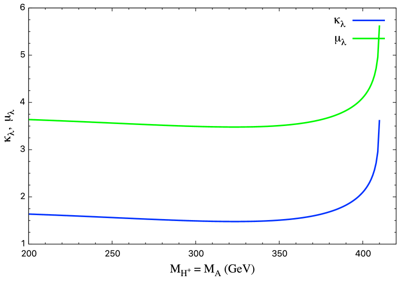
Figure 4: The ratios $\kappa_{\lambda}=\lambda^{(0)+(1)}_{H_{1}H_{1}H_{1}}/(\lambda_{HHH})_{\rm SM}$ (with $(\lambda_{HHH})_{\rm SM}\cong 32\,{\rm GeV}$) and $\mu_{\lambda}=\lambda^{(0)+(1)}_{H_{1}H_{1}H_{1}H_{1}}/(\lambda_{HHHH})_{\rm SM}$ (with $(\lambda_{HHHH})_{\rm SM}\cong 0.0323$) as a function of $M_{H^{\pm}}=M_{A}$. The sharp rise starting near $M_{H^{\pm}}=370\,{\rm GeV}$ is an artifact of $M_{H^{\prime}}$ starting its dive to zero.

This effect of the sum rule is seen numerically in Table 1 where we list triple and quartic couplings for three extreme values of $M_{H^{\pm}}$ in Fig. 4. The $V_{0}$ contribution to $\lambda_{H_{1}H_{1}H_{2}}$ is small and its $V_{1}$ contribution would vanish were it not for the fact that $m_{t}^{2}=\Gamma_{t}\Phi_{1}^{\dagger}\Phi_{1}$ contains a linear term in $H^{\prime}$. On the other hand, for almost the entire $M_{H^{\pm}}$ range, the contributions to $\lambda_{H_{1}H_{2}H_{2}}$ listed in the table are of normal size, ${\cal O}(\lambda_{HH^{\prime}H^{\prime}}=M_{H_{2}}^{2}/v$). The interesting question of the effect this large coupling has on the production rate of $pp\to H_{2}H_{2}$ is beyond the scope of this paper.

$M_{H}\cong M_{H_{1}}$	$M_{H^{\pm}}=M_{A}$	$M_{H^{\prime}}$ ($M_{H_{2}}$)	$\lambda^{(0)+(1)}_{H_{1}H_{1}H_{1}}$	$\kappa_{\lambda}$
125	200	532 (534)	51.9	1.64
125	400	301 (314)	66.6	2.10
125	410	115 (214)	115	3.63
$\lambda^{(0)+(1)}_{H_{1}H_{1}H_{2}}$	$\lambda_{HH^{\prime}H^{\prime}}$	$\lambda^{(0)+(1)}_{H_{1}H_{2}H_{2}}$	$\lambda^{(0)+(1)}_{H_{1}H_{2}H_{2}}/\lambda_{HH^{\prime}H^{\prime}}$
3.84	1151	1252	1.09
2.62	367	510	1.39
7.92	54.1	349	6.46
$\lambda^{(0)}_{H_{1}H_{1}H_{1}H_{1}}$	$\lambda^{(1)}_{H_{1}H_{1}H_{1}H_{1}}$	$\lambda^{(0)+(1)}_{H_{1}H_{1}H_{1}H_{1}}$	$\mu_{\lambda}$
$-0.942\times 10^{-3}$	0.118	0.117	3.64
0.0139	0.118	0.132	4.10
0.0634	0.118	0.182	5.63

Table 1: Selected cubic and quartic couplings of the 125 GeV Higgs boson. Input masses are $M_{H}\cong M_{H_{1}}$ and $M_{H^{\pm}}=M_{A}$, with $M_{H^{\prime}}$ taken from the sum rule Eq. (35) as explained in the text; $M_{H_{2}}$ is the corresponding $C\!P$-even eigenvalue at one-loop order; $\tan\beta=0.50$, and the misalignment angle $\delta=0.0039$, 0.0115, 0.0323 for $M_{H^{\pm}}=200$, 400, $410\,{\rm GeV}$. Couplings $\lambda^{(0)}$ and $\lambda^{(1)}$ are contributions from the one-loop improved $V_{0}$ and full one-loop $V_{1}$ potentials. Comparisons are made to the Standard Model ($\kappa_{\lambda}=\lambda^{(0)+(1)}_{H_{1}H_{1}H_{1}}/(\lambda_{HHH})_{\rm SM}$ and $\mu_{\lambda}=\lambda^{(0)+(1)}_{H_{1}H_{1}H_{1}H_{1}}/(\lambda_{HHHH})_{\rm SM}$) or to tree-level values ($\lambda^{(0)+(1)}_{H_{1}H_{2}H_{2}}/\lambda_{HH^{\prime}H^{\prime}}$). Masses and cubic couplings are in GeV units.

The value of the triple-Higgs coupling $\lambda^{(0)+(1)}_{H_{1}H_{1}H_{1}}$ in the GW-2HDM is close to its small SM value. As can be seen in Refs. [16, 17, 18], $\kappa_{\lambda}\simeq 1.6$–$3.6$ corresponds to $\sigma(pp\to HH)=15$–$20\,{\rm fb}$. This is the absolute minimum value of the di-Higgs production cross section for $\sqrt{s}=13$–$14\,{\rm TeV}$ at the LHC. Because the sum rule (1) is independent of the number or type of Higgs multiplets in the GW model, this result is true of all of them.

We are aware that there are many theoretical studies of the cubic and even quartic Higgs couplings — in the context of one-doublet models, multi-doublet models, models with extra singlet “Higgses”, and so on — many more studies than we can note here. We apologize to their authors for not citing them. At perhaps the simplest level, this is the problem of the shape of the potential of the Higgs boson itself, specifically, what are $\lambda_{HHH}$ and $\lambda_{HHHH}$? One recent paper [6] studied a variety of new physics scenarios, their effect on these couplings, and the prospect of distinguishing them at the $14\,{\rm TeV}$ High Luminosity LHC (HL-LHC), the $27\,{\rm TeV}$ High Energy LHC (HE-LHC) and the $100\,{\rm TeV}$ Future Circular Hadron Collider (FCC-hh). These authors considered, inter alia, a Coleman-Weinberg-like potential. Compared to the SM values, they found $\kappa_{\lambda}=5/3$ and $\mu_{\lambda}=11/3$. These are close to our calculated values of $\kappa_{\lambda}$ and $\mu_{\lambda}$ in Fig. 4 below $M_{H^{\pm}}=M_{A}\cong 370\,{\rm GeV}$. According to the analysis in Ref. [6] of di-Higgs and tri-Higgs observability at the upgraded LHC and the FCC-hh, the HE-LHC is needed to detect and distinguish the triple Higgs coupling of the GW-2HDM and the FCC-hh is needed for the quartic coupling. This is a gloomy prospect.

IV. Testing Gildener-Weinberg at the LHC

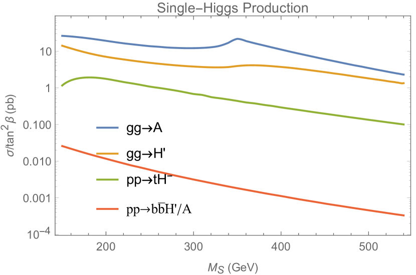
Figure 5: The cross sections for $\sqrt{s}=13\,{\rm TeV}$ at the LHC for single Higgs production processes in the alignment limit ($\delta\to 0$) of the GW-2HDM with the dependence on $\tan\beta$ scaled out. Both charged Higgs states are included in $pp\to tH^{-}$. From Ref. [5].

Much more immediately promising avenues of attack on GW models are searches for the new charged and neutral Higgs bosons that lie below 400–$500\,{\rm GeV}$. In the GW-2HDM, the new scalars are just $H^{\pm}$, $A$ and $H_{2}$. Assuming as we have that $M_{H^{\pm}}=M_{A}$, the principal search modes are:

$$H^{\pm} \to t\bar{b}\,(b\bar{t})\,\,{\rm and}\,\,W^{\pm}H_{2};$$ (62)

$$A \to b\bar{b},\,\,t\bar{t}\,\,{\rm and}\,\,ZH_{2};$$ (63)

$$H_{2} \to b\bar{b},\,\,t\bar{t}\,\,{\rm and}\,\,ZA,\,W^{\pm}H^{\mp}.$$ (64)

Their main production cross sections at the 13 TeV LHC were discussed in Ref. [5] and they are displayed in Fig. 5 with the dependence on $\tan^{2}\beta$ scaled out. There seem to have been but a few searches for $pp\to H_{2}\,\,{\rm or}\,\,A\to b\bar{b}$, presumably because of the overwhelming continuum $b\bar{b}$ production. One recent search by CMS for a $C\!P$-even or odd scalar with $M_{b\bar{b}}=50$–$350\,{\rm GeV}$ and produced at high-$p_{T}$ is reported in Ref. [19]. No significant excess over SM backgrounds was found. For $M_{H_{2},A}=200$–$350\,{\rm GeV}$, the 95% CL limits are $\sigma(pp\to H_{2},A)B(H_{2},A\to b\bar{b})\simeq 200$–$300\,{\rm pb}$ which translates into upper limits $\tan\beta\simeq 3$–6. It is important to note that the decays $H_{2},A\to W^{+}W^{-},\,\,ZZ$ and $H^{\pm}\to W^{\pm}Z$ are highly suppressed in GW models by the near alignment of the SM Higgs $H\cong H_{1}$. Likewise, alignment strongly suppresses $H_{2},A\to ZH$ and $H^{\pm}\to W^{\pm}H$. Seeing these decay modes from a new, heavier spinless boson would be significant, if not fatal, blows to GW models.

The following is a summary of the current experimental situation for the new Higgs bosons’ dominant decay modes:

• The CMS search at $8\,{\rm TeV}$ for $H^{\pm}\to t\bar{b}$ [12] restricted $\tan\beta\mathrel{\hbox to0.0pt{\raise 2.20013pt\hbox{$<$}\hss}{\lower 2.20013pt\hbox{$\sim$}}}0.5$ for our type-I GW-2HDM with $180\,{\rm GeV}<M_{H^{\pm}}<550\,{\rm GeV}$ [5]. Searches at $13\,{\rm TeV}$ for $H^{\pm}\to t\bar{b}$ by ATLAS [13] and CMS [20] extend down to $M_{H^{\pm}}=200\,{\rm GeV}$, but do not yet have the sensitivity to reach $\sigma(pp\to tH^{\pm})=0.50\,{\rm pb}$ ($0.033\,{\rm pb}$) expected at $200\,{\rm GeV}$ ($500\,{\rm GeV}$) for $\tan\beta=0.50$ and $B(H^{\pm}\to t\bar{b})=1$. At $M_{H^{\pm}}=400\,{\rm GeV}$ in the GW-2HDM, Fig. 3 gives $M_{H_{2}}=314\,{\rm GeV}$, while at $M_{H^{\pm}}=408\,{\rm GeV}$, it gives $M_{H_{2}}=247\,{\rm GeV}$. Between these two mass points, the $H^{\pm}\to W^{\pm}H_{2}$ decay rate increases by a factor of 70, overwhelming the $H^{\pm}\to t\bar{b}$ decay rate; see item (3) below. The two processes $g\bar{b}\to H^{+}\bar{t},\,H^{+}\to t\bar{b}$ and $g\bar{b}\to H^{+}\bar{t},\,H^{+}\to W^{+}H_{2}$, with $H_{2}\to b\bar{b}$, have the same final state. Hence, $H^{+}\to W^{+}H_{2}$ may unintentionally be included in a search for $H^{+}\to t\bar{b}$. Even if that happened, the model expectation $\sigma(g\bar{b}\to H^{+}\bar{t})=0.075\,{\rm pb}$ for $M_{H^{\pm}}\simeq 400\,{\rm GeV}$ and $\tan\beta=0.5$ is well below the 95% CL limits $\simeq 0.5\,{\rm pb}$ (ATLAS) and $0.7\,{\rm pb}$ (CMS). There appear to be no dedicated searches released for $H^{\pm}\to W^{\pm}H_{2}\to\ell^{\pm}b\bar{b}$ and for $H_{2}\to W^{\pm}H^{\mp}\to\ell^{\pm}t\bar{b}$.

  $M_{A}=M_{H^{\pm}}$	$M_{H_{2}}$	ATLAS	CMS	GW-2HDM
  400	300	255	75	65
  300	500	105	50	100

  Table 2: 95% CL upper limits on $\sigma(pp\to A(H_{2}))\,B(A(H_{2})\to ZH_{2}(A))B(H_{2}(A)\to\bar{b}b)$ via gluon fusion from ATLAS [21], CMS [22] and GW-2HDM calculations for two cases of large $M_{A}$ and $M_{H_{2}}$. The CMS limits include $B(Z\to e^{+}e^{-},\,\mu^{+}\mu^{-})$; the ATLAS limits and GW-2HDM predictions do not. Masses are in GeV and $\sigma B$ in femtobarns. $M_{A}=M_{H^{\pm}}$ is assumed and $M_{H_{2}}$ is taken from Fig. 3 as explained in the text. Model cross sections are taken from Fig. 5 multiplied by $\tan^{2}\beta=0.25$.

• CMS recently reported a search for a $C\!P$-even or odd scalar $\varphi$ with mass in the range 400 to $700\,{\rm GeV}$ and decaying to $t\bar{t}$ [23]. Results were presented in terms of allowed and excluded regions of the “coupling strength” $g_{\varphi}=\lambda_{\varphi t\bar{t}}/(m_{t}/v)$ and for fixed width-to-mass ratio $\Gamma_{\varphi}/M_{\varphi}=0.5$–25%. In the GW-2HDM, $g_{\varphi}=\tan\beta$. For the $C\!P$-odd case, $\varphi=A$, with $400\,{\rm GeV}<M_{A}<500\,{\rm GeV}$ and all $\Gamma_{A}/M_{A}$ considered, the region $\tan\beta<0.5$ is not excluded. This is possibly due to an excess at $400\,{\rm GeV}$ that corresponds to a global (local) significance of $1.9\,\,(3.5\pm 0.3)\,\sigma$ for $\Gamma_{A}/M_{A}\simeq 4\%$. Ref. [23] also notes that $t\bar{t}$ threshold effects may account for the excess.

• Searches for $pp\to A(H_{2})\to ZH_{2}(A)\to\ell^{+}\ell^{-}b\bar{b}$ via gluon fusion have been reported by ATLAS [21] and CMS [22]. Two examples of observed 95% upper limits on cross sections and the corresponding GW-2HDM predictions are given in Table 2. A word of caution is in order here: These decay rates are dominated by the emission of longitudinally-polarized weak bosons and are proportional to $p^{3}/M_{W,Z}^{2}$, hence sensitive to the available phase space.

At the LHC there are now $140\,{\rm fb}^{-1}$ of $pp$ collision data at $13\,{\rm TeV}$ from Run 2 and another $200\,{\rm fb}^{-1}$ at $14\,{\rm TeV}$ are expected from Run 3 by the time it concludes at the end of 2024. With masses in the range $200$–$500\,{\rm GeV}$, GW Higgs production rates are $\sigma(pp\to H^{+}+H^{-})=(0.1-1.0)\,{\rm pb}\times\tan^{2}\beta$, $\sigma(pp\to A)=(4.0-20)\,{\rm pb}\times\tan^{2}\beta$ and $\sigma(pp\to H_{2})=(2.0-7.0)\,{\rm pb}\times\tan^{2}\beta$. Thus, unless $\tan\beta\mathrel{\hbox to0.0pt{\raise 2.20013pt\hbox{$<$}\hss}{\lower 2.20013pt\hbox{$\sim$}}}0.2$, there will be anywhere from $10^{3}$ to several $10^{6}$ of these GW Higgs bosons produced by the end of Run 3. Given the large SM production of $b\bar{b}$, direct detection of $H_{2}\to b\bar{b}$ via gluon fusion is the most difficult. There is no doubt that improved sensitivity in the low-mass region of $H^{\pm}\to t\bar{b}$ is needed to access the expected cross sections. The decays $A({\rm or}\,\,H_{2})\to ZH_{2}({\rm or}\,\,A)\to\ell^{+}\ell^{-}b\bar{b}$, $H^{\pm}\to W^{\pm}H_{2}\to\ell^{\pm}b\bar{b}+\kern 2.5pt\raise 0.77496pt\hbox{$/$}\kern-6.99997ptE_{T}$ are helped by the narrow $b\bar{b}$ resonance and lepton kinematics. They may be easier than $H^{\pm}\to t\bar{b}$, but they cover a slimmer portion of ($M_{H^{\pm}},M_{A},M_{H_{2}}$)-space, the upper and lower ends of the allowed $M_{H^{\pm}}=M_{A}$ region.

References

[1]
E. Gildener and S. Weinberg, “Symmetry Breaking and Scalar Bosons,” Phys. Rev.D13 (1976) 3333.
[2]
J. S. Lee and A. Pilaftsis, “Radiative Corrections to Scalar Masses and
Mixing in a Scale Invariant Two Higgs Doublet Model,” Phys. Rev.D86 (2012) 035004, 1201.4891.
[3]
S. R. Coleman and E. J. Weinberg, “Radiative Corrections as the Origin of
Spontaneous Symmetry Breaking,” Phys. Rev.D7 (1973)
1888–1910.
[4]
K. Hashino, S. Kanemura, and Y. Orikasa, “Discriminative phenomenological
features of scale invariant models for electroweak symmetry breaking,” Phys. Lett.B752 (2016) 217–220,
1508.03245.
[5]
K. Lane and W. Shepherd, “Natural stabilization of the Higgs boson’s mass
and alignment,” Phys. Rev.D99 (2019), no. 5, 055015,
1808.07927.
[6]
P. Agrawal, D. Saha, L.-X. Xu, J.-H. Yu, and C. P. Yuan, “Shape of Higgs
Potential at Future Colliders,”
1907.02078.
[7]
J. F. Gunion and H. E. Haber, “The CP conserving two Higgs doublet model: The
Approach to the decoupling limit,” Phys. Rev.D67 (2003)
075019, hep-ph/0207010.
[8]
S. Weinberg, “A Model of Leptons,” Phys.Rev.Lett.19 (1967)
1264–1266.
[9]
B. Bellazzini, C. Csaki, J. Hubisz, J. Serra, and J. Terning, “A Higgslike
Dilaton,” Eur. Phys. J.C73 (2013), no. 2, 2333,
1209.3299.
[10]
S. L. Glashow and S. Weinberg, “Natural Conservation Laws for Neutral
Currents,” Phys. Rev.D15 (1977) 1958.
[11]
G. C. Branco, P. M. Ferreira, L. Lavoura, M. N. Rebelo, M. Sher, and J. P.
Silva, “Theory and phenomenology of two-Higgs-doublet models,” Phys.
Rept.516 (2012) 1–102,
1106.0034.
[12]CMS Collaboration, V. Khachatryan et. al., “Search for a charged
Higgs boson in pp collisions at TeV,” JHEP11
(2015) 018, 1508.07774.
[13]ATLAS Collaboration, M. Aaboud et. al., “Search for charged Higgs
bosons decaying into top and bottom quarks at = 13 TeV with the
ATLAS detector,” JHEP11 (2018) 085,
1808.03599.
[14]
R. A. Battye, G. D. Brawn, and A. Pilaftsis, “Vacuum Topology of the Two
Higgs Doublet Model,” JHEP08 (2011) 020,
1106.3482.
[15]
A. Pilaftsis, “On the Classification of Accidental Symmetries of the Two
Higgs Doublet Model Potential,” Phys. Lett.B706 (2012)
465–469, 1109.3787.
[16]CMS Collaboration, A. M. Sirunyan et. al., “Combination of
searches for Higgs boson pair production in proton-proton collisions at
13 TeV,” Phys. Rev. Lett.122 (2019), no. 12,
121803, 1811.09689.
[17]ATLAS Collaboration, G. Aad et. al., “Combination of searches for
Higgs boson pairs in collisions at 13 TeV with the ATLAS
detector,” Phys. Lett.B800 (2020) 135103,
1906.02025.
[18]
A. Carvalho, M. Dall’Osso, P. De Castro Manzano, T. Dorigo, F. Goertz,
M. Gouzevich, and M. Tosi, “Analytical parametrization and shape
classification of anomalous HH production in the EFT approach,”
1608.06578.
[19]CMS Collaboration, A. M. Sirunyan et. al., “Search for low-mass
resonances decaying into bottom quark-antiquark pairs in proton-proton
collisions at 13 TeV,” Phys. Rev.D99 (2019),
no. 1, 012005, 1810.11822.
[20]CMS Collaboration, A. M. Sirunyan et. al., “Search for a charged
Higgs boson decaying into top and bottom quarks in events with electrons or
muons in proton-proton collisions at = 13 TeV,” JHEP01 (2020) 096,
1908.09206.
[21]ATLAS Collaboration, M. Aaboud et. al., “Search for a heavy Higgs
boson decaying into a boson and another heavy Higgs boson in the
final state in collisions at TeV with the
ATLAS detector,” Phys. Lett.B783 (2018) 392–414,
1804.01126.
[22]CMS Collaboration, A. M. Sirunyan et. al., “Search for new
neutral Higgs bosons through the H ZA process in pp collisions at 13 TeV,”
1911.03781.
[23]CMS Collaboration, A. M. Sirunyan et. al., “Search for heavy
Higgs bosons decaying to a top quark pair in proton-proton collisions at
13 TeV,”
1908.01115.