Leray turbulence: what can we learn from acceleration compared to velocity
Abstract
In a recent paper we presented evidence for the occurence of Leray-like singularities with positive Sedov-Taylor exponent in turbulent flows recorded in Modane’s wind tunnel, by looking at simultaneous acceleration and velocity records. Here we use another tool which allows to get other informations on the dynamics of turbulent bursts. We compare the structure functions for velocity and acceleration in the same turbulent flows. This shows the possible contribution of other types of self-similar solutions because this new study shows that statistics is seemingly dominated by singularities with small positive or even negative values of the exponent , that corresponds to ”weakly singular” solutions with singular acceleration, and regular velocity. We present several reasons explaining that the exponent derived from the structure functions curves, may look to be negative.
I Introduction
Many natural and man-made flows have typically large to very large Reynolds number and negligible Mach number, the limit we shall deal with. The neglect of viscosity and compressibility leads to the Euler equations Euler ,
| (1) |
and
| (2) |
where is for the time derivative, the vector is the local value of the fluid velocity at time , boldface being for vectors, and is the pressure, a gauge function allowing to satisfy the condition of incompressibllity (2). The nabla sign is for the gradient with respect to coordinate and the mass density has been set to .
The next question is: what is predicted by Euler equations? We do not know yet if smooth and bounded velocity fields in three space dimensions always yield a smooth solution at any later time.
In 1934 Leray leray suggested to explain the irregularity of turbulent flows by a loss of predictability linked to the occurrence of singularities in the solutions of this evolution equations. Such singularities would forbid to continue the solution afterwards within the framework of deterministic fluid equations. Leray went further than that and wrote down the equation for self-similar solutions of the Navier-Stokes equation (including the viscosity - see below) describing the evolution from smooth initial data to a solution singular at one point of space and time (his equation (3.11)).
We have recently presented evidence for the occurrence of Leray-like singularities in a high-speed wind tunnel, as recorded by a hot wirePC . Such singularities manifest themselves by the property that large values of the velocity fluctuations are correlated to large values of the acceleration at the same point and same time, those large fluctuations being linked by a relation of the form
| (3) |
On the contrary Kolmogorov (1941) scaling law yields , and so predicts a vanishing acceleration when the velocity is large and conversely a large acceleration and a small velocity at the same point of space-time in the fluid, exactly the opposite of what is observed. From this observation we inferred that the data are quantitatively well explained by the occurrence of Leray-like singularities of Euler fluid equations with exponents derived by assuming scaling laws coherent with the local conservation of energy, a point detailed just below.
As did Leray leray let us suppose there is a singularity in finite time by the evolution of the flow velocity and that this singularity is of the self-similar type. The corresponding solution of the Euler equations is of the type
| (4) |
where is the time of the singularity (set to zero afterwards), where and are exponents to be found and where is to be derived by solving Euler equations. Such a velocity field is a solution of Euler equations if
| (5) |
In PC our analysis of the experiments performed in Modane pointed to values of and both close to . We argued that those values could be associated to two (different) conservation laws, each one corresponding to a set of exponents, one is which ensures the conservation of the circulation around the the singularity, the other one providing the conservation of energy in the singular domain is and , which is related to the Sedov-Taylor scaling. The former set leads to , the latter, which leads to , in slightly better agreement with the data than .
Here we look at other possible values for the exponents . At this time it is unknown if an unique value of the exponents exists, as resulting from the equation of self-similarity or if more than a single value exists. Looking carefully to the experimental data, it appears that the divergence of the velocity, if there is any, is fairly weak. At first sight comparing the amplitude of the velocity fluctuations and of the acceleration versus time, we observe that the former are noticeably smaller than the latter (in units of their respective r.m.s), as illustrated in Fig.1 showing the temporal traces of acceleration and velocity in the case of a medium intensity burst. Note that the existence of several values for the exponents is all the same compatible with the relation (3) found to agree very well with the experimental data of Modane, because the analysis done in ref PC correlates large values of the acceleration and large values of the velocity at the same point in space-time. It could well be that (3) does not describe all fluctuations of the velocity for a given value of the acceleration that contribute to averages so that the singularities considered in PC are only part of a larger set of singular solutions, with different values of the exponent , in the range . The latter condition is necessary to yield a singularity of the acceleration, as observed, because the exponent for the time dependence of the acceleration is and has to be positive. Therefore we argue that it is even possible that the exponent is negative for some solutions of the Euler-Leray equation (8). Actually we show that a subset of singular solutions with negative values
| (6) |
is consistent with the observation that the structure function built with the velocity does not seem to become singular at short distances, whereas the structure function built with the acceleration becomes more and more peaked near as the exponent increases. This result allows to define such ”weak” singularities as singularities of the acceleration but not of the velocity. They are obviously unseen when one focus on the correlation of the largest values of the observed acceleration and velocities, while the present study comparing the structure functions for velocity and acceleration implies that statistics is dominated by events with small positive or even slightly negative values of .
It could also be that even in presence of solutions with positive, the statistical analysis performed here select another family of solutions than inPC , a subtle point related to the dilation invariance of Euler equation which have a family of solutions, , parametrized by their amplitude , as discussed in Sec. III.2. Below we point out that close to a singular point, a self-similar solution with given () values behaves differently than the one with (), so that an experiment sensitive to the transient behavior towards the singular time may lead the observer to conclude that solutions with negative values exist in the flow although it is false. We show that such misleading effect could result from the existence of a large proportion of weak amplitude singularities as compared to large amplitude ones.
There is another point related to what we call ”singular event”. Such an event is seen as a large fluctuation in the time records of velocity but such records deal with fluid mechanics of real fluids. It means two things. First viscosity should play a role, likely (but not necessarily, see below) by smoothing the singularity when its typical size becomes too small. Because this happens when the velocity and acceleration become very large, the net effect of the viscosity should be to quell the growth of the velocity and of the acceleration. This is in fair agreement with the fact that the short distance behavior of the structure function is less divergent than predicted by the inviscid Euler-Leray equations. Another property of the real data is that after the singularity takes place a decay phase, see the example shown in Fig.1, that is, at least partly recorded as a large fluctuation. This ”post singularity” dynamics depends on the way the system crosses the singularity, which relies in particular on dissipative effects induced either by viscosity or compressibility and emission of sound. How such post singularity events contribute to the structure function is unknown, but it is reasonable to assume that they do it with exponents smaller than the pre-singularity part just because this relies on dissipation allowing to cross the inviscid singularity time.
(a)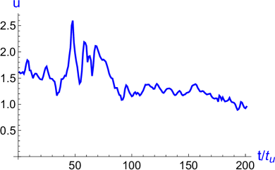
(b)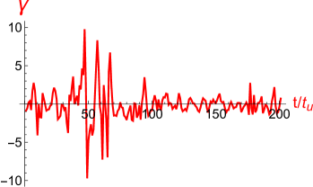
With the variable , the Euler equations become a set of equations (the Euler-Leray equations) for . The incompressibility condition is
| (7) |
There exists also an extended version of the similarity equation with an explicit time dependent part. This is found by using as variable and by keeping a velocity field depending on via the stretched radius . This yields the modified Euler-Leray equation
| (8) |
The present note aims at giving support to the link between the occurrence of singularities and the observation of strong gradients. This relies on a precise analysis of experimental records of velocity fluctuations in Modane’s wind tunnel. Instead of conditioning the measured values of the velocity to the one of acceleration, as done in PC , we introduce in next section a statistical analysis taking into account the random occurrence in space and time of Leray singularities. Assuming that self-similar solutions are mainly responsible for the striking divergence of high-order structure functions at small spatial scales, we derive an estimation of their power-law dependence on the form . We also indicate how the space-time density of singular events can be expressed in terms of the parameters of turbulence. This problem is discussed at the end of this subsection. In subsection II.2 we present the real structure functions deduced from the data taken in Modane’s wind tunnel, namely the same data as in PC . The striking results are discussed and interpreted in Sec.III taking into account the role of the viscosity in the ultimate stage of singularity formation (a question studied in more details in PC ), the role of the dilation invariance on the measurements, and other possible causes.
II Structure functions and large fluctuations
We look at the structure functions traditionally defined as an ensemble average of the spatial increment of a vector field in between two points and , for an arbitrary time, the same time. The ensemble average becomes a sliding average over when the turbulence is homogeneous, a condition assumed hereafter, then structure functions only depend on the distance . One has
| (9) |
where . We consider such moments associated to the velocity, namely for , and also to the Eulerian acceleration defined as .
For large , the structure functions tends to a constant, see Figs.2, given by the sum . In the following we focus on the behavior of at short distance for even . As we noticed in ref PC , the velocity fluctuations are not very far from being Gaussian, which makes large fluctuations quite unlikely. On the contrary the probability distribution of the acceleration has much wider wings than a Gaussian, that gives them a fairly large probability of being big. Since we look for properties linked to singularities, and so to big fluctuations, we thought it better to look at the structure function built with the acceleration field instead of the velocity field. Whereas we found that the velocity fluctuations hardly show any trace of singular events in the -dependence of the structure function, we found that, on the contrary, the structure functions built with the acceleration show a clear, not to say obvious, evidence of singularities in the short range behavior of the structure function, see Figs.2.
II.1 Contribution of quasi-singular solutions
Let us give first an estimate of the contribution of quasi-singular events to structure functions. By such a quasi-singular event we mean a solution of the evolution equation (Euler equation in fluid mechanics of inviscid fluids) becoming singular in finite time at a given point of space and time. This is said to be quasi-singular because it cannot be a singularity in the exact mathematical sense in real life: Euler equations have to break down at small scales, either because of the effect of viscosity if the Reynolds number in the Euler singularity decreases too much, or if this is not the case (no decrease of the Reynolds number), other physical effects like compressibility should become relevant. We comment on those possibilities at the end of this section including our study based on experimental observations.
In the following we drop the boldface notation for the vector field, and denote as the field under consideration to remind that we shall focus on acceleration. Close to a singular event of type (see just below) occurring at the space-time point , the solution of the fluid equations is of the form where is singular at by definition, and is a set of parameters taking into account the possibility that there is more than one kind of singular solution, either because of a multiplicity of solutions like in the eigenvalues of a standard matrix or because of various symmetries of those solutions, either geometrical (by rotation) or because of the dilation symmetries of the Euler equations. For example in the case of a solution like (4) with given exponents and dilation parameter , setting , the acceleration close to a singular event of -type near can be written as
| (10) |
Because the singularities are localized in space and time, one does not expect them to overlap. Instead one even expects that they tend to interact by repulsion because the growth of a singularity exhausts the local possibility of another one growing nearby at about the same time, which induces a kind of repulsion between singularities CJ . To streamline the explanations we shall assume that singularities do not interact at all so that the velocity field created by all singularities is a superposition of independent singular solutions with random choices of and with a given density in space and time. Correlated singularities should be taken into account, but we skip them because it would add lot of difficulties for estimating compared to the rough one presented now.
We make the hypothesis that high order moments ( large) are dominated by the contribution of singularities. If the parameters labelled form a discrete set , the structure function can be approximated by a sum of over space-time domains labelled by the discrete index ,
| (11) |
Going to a continuum of possible quasi-singularities, let define as the density of quasi-singularity per unit time and unit volume. The mean number of quasi-singularities per unit time and unit volume, is
| (12) |
which has the physical dimension of a frequency times an inverse volume. The sum (11) becomes
| (13) |
Equations (11) or (13) assume implicitly, something far from obvious, that singular solutions of the equation have a basin of attraction of finite volume in phase space. This implies in particular that, by linearizing the Euler-Leray equations in their form (8), the solution representing a singularity is stable with respect to small perturbations (we mean stable in the usual sense that small perturbations decay to zero as the ”logarithmic” time tends to infinity as tends to ). Notice that contrary to the original Euler equations, the Euler-Leray equations being not reversible with respect to time may have stable solution in the ordinary sense, namely be attracting in all directions of phase space.
Let us note that the above description takes out the important question of the space-time density , and how depends on the parameters of turbulence. To answer this we need to have in the theory parameters allowing to build a quantity with the physical dimension of a space-time density, namely , where is a length scale and a time scale. In Kolmogorov theory, turbulence in the so-called inertial domain is characterized by the power dissipated per unit mass, with the physical dimension . No quantity with the dimension can be built by taking a power of , assuming that viscosity does not play a role in the formation of singular events, because they result from the inviscid dynamics only. The Kolmogorov scaling for the rate of energy dissipation by transfer of energy toward the small scales makes the quantity denoted by Kolmogorov as the only scaling parameter for turbulent velocity field with ”inviscid” dissipation. This is independent of the precise mechanism of this dissipation, be it by random cascade toward smaller and smaller ”vortices” continuously distributed in space or, as we shall consider it, by singular events distributed randomly in space and time. Therefore the parameter permitting to find the density of singular events in space and time cannot be linked to viscosity which is relevant near the end of the singularity formation only. This supplementary parameter must somehow depend only on the characteristics of the inviscid flow. Besides , there are of course many parameters describing the turbulent fluctuations, like the mean square velocity fluctuation, or powers of the gradients of this velocity field (still partly taken into account by ). It could be pertinent to take as another parameter the density of turbulent kinetic energy, namely half of the mean square fluctuating velocity. This parameter is the of the - theory Keps . When seen from the point of view of the Kolmogorov-Obukhov spectrum, this parameter is also needed to make finite the total energy in the spectrum, as necessary. Therefore we shall choose as dimensionalizing parameters and . It follows from this choice that a typical length and time scales of turbulence are
| (14) |
Thanks to both scales it makes sense, for a given turbulent state to consider singularities with a space-time density defined intrinsically as proportional to , or
| (15) |
without explicitly relying on the size of the turbulent channel (for instance).
At this step, because we ignore the explicit form of the singular solutions of Euler or Navier-Stokes equations, it is not possible to compute explicitly the integral on the right-hand side of (13). However it is possible to find how it behaves as a function of , because depends on its arguments as prescribed by the self-similar dependence (10). We set and leave the exponents and undefined first in this estimate, in other words we consider a single type of singularity associated to a given set of exponents . In the collapsing region we have the scaling , and . Inverting the relation between and one finds
| (16) |
The volume of the domain is of order . Substituting those power laws in the right-hand side of equation (11), one finds for the contribution of singularities with given exponents , to at short distance
| (17) |
for the structure functions associated to the acceleration, and for the structure functions associated to the velocity
| (18) |
Expression (17) shows that as gets larger than , diverges formally as tends to zero. Similarly diverges formally for .
With the Sedov-Taylor exponents, diverges for , and diverges for . Note first that a divergence of at is formally inconsistent with the definition (9) which should be zero at . The viscosity effect is often invoked to explain the regularization of the solution just before the divergence, however, as discussed in Sec.III.1, with the Sedov-Taylor exponents the viscosity effect is not sufficient to dissipate the energy in the singular space-time domain and to stop the evolution to the singularity.
Besides this determination of a critical value of such that changes behavior near , which is not very well defined from the experimental data, there is also a consequence of the scaling law in equation (17), namely that the exponent is an affine function of , a result confirmed by the experiment, see Fig.3 in the next subsection.
II.2 Experimental results
We use the same data as in PC , namely those recorded from hot wires in the wind-tunnel of Modane, by Y. Gagne et al. in the s expmod -exp2mod , and also more recent ones obtained in 2014 in the framework of a ESWIRP European projectmickael . In both cases we got records from a single probe. If the probe is localized at , the measured velocity at time is
where is the mean velocity of the turbulent flow. We assume that the Taylor approximation of frozen turbulence is valid, then the spatial dependence of the structure functions is replaced by a temporal dependence, with . In the following the velocity fluctuation recorded by the hot wire, labelled , is assumed to be the longitudinal component of , and the Eulerian acceleration, labelled , is the quantity calculated from the increments of this velocity, , which approximates the partial derivative of the longitudinal velocity if the sampling time is small enough. The former measurements were taken in the return vein of the Modane wind tunnel, with Reynolds number , mean velocity about m/s, r.m.s. m/s, sampling frequency KHz and Kolmogorov time estimated as ms. In the latter case the data were recorded behind a grid put in the test section of the wind tunnel, the Reynolds number was about five times smaller, , and the sampling frequency KHz was ten times larger than in the ancient record. The statistical study based on structure functions which is described in this section stem from the ten minutes record of Y. Gagne in the s, however we have checked that recent and ancient data fully agree.
We found that the structure functions for the velocity and acceleration reveal a very different behavior at large values of , especially for small spatial scales (close to the Kolmogorov scale), as shown in Figs.2 where the curves for the acceleration display a maximum increasing strongly with the order , although the structure functions for the velocity grow monotonically before they reach their constant asymptotic value for much larger than the correlation time. We note that the maxima of curves (b) occur practically at the Kolmogorov time (). We also observe that tends (rapidly) to a constant as a function of r, as r increases. This short distance correlation of the acceleration agrees with the hypothesis of statistically independent singularities made in II.1.
(a)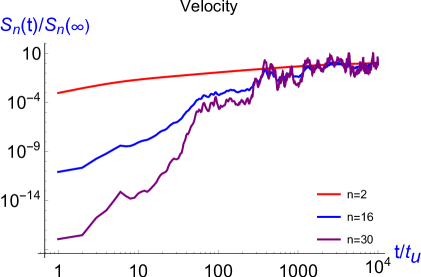 (b)
(b)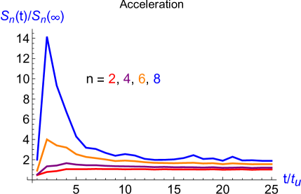
(a) 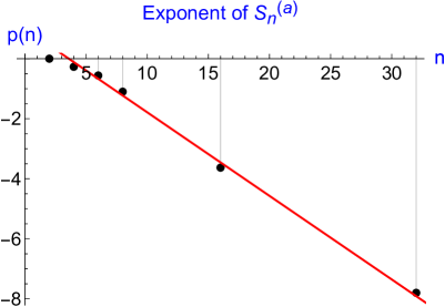 (b)
(b)
If Sedov-Taylor exponents were the only ones contributing to , a peak should appear in structure function for acceleration and velocity at large . Therefore, although singularities with Sedov-Taylor exponents should be present in the turbulent flow, the very different behavior of curves (a) and (b) in Figs.2 indicates that these solutions have small contribution in the structure functions, that enforce the hypothesis made above, of multi-type singularities. More precisely one may deduce an effective exponent from the sharp growth of experimental curves (b) as decreases. Focusing on the right part of the peaks in the range , and setting
| (19) |
we measure an exponent . We find that it decreases linearly with , as shown in Fig.3, as
| (20) |
Comparing with the formal expression (17), we conclude that, if singular events are responsible for the striking behavior of curve (b), they correspond in average to exponents
| (21) |
As written in the introduction, negative values of , with (6) fulfilled, may correspond to self-similar solutions associated to what we called ”weak” singular events in the introduction, they have singular acceleration but regular velocity. Therefore equation ( 21) open the perspective of the existence of weak singularities in the turbulent flow of Modane’s but it also deserves some remarks.
III Discussion
These ”weak” events can have several reasons to appear in the recorded signal. Those noted below deserve to be considered, beyond the fact that all of them are able to explain that the exponent derived from the experimental curves, is negative.
III.1 Role of viscosity for Sedov-Taylor singular events
Before focusing on possible multiplicity of values, let us consider singularities with Sedov-Taylor exponents. We are going to show that only a small part of the energy is dissipated via viscosity effects in these structures. As generally understood viscosity enters into play in the ultimate stage of the blowing up of the solution when approaches the formal value, preventing the growth of the solution. First let us notice that if this is true, then viscosity is expected to act also after when the fluctuations remain large, see Fig.1, that should make post-collapse peaks in the signal contributing to the structure function, including at r small, in an unknown (yet) way. Secondly, we claim that even though it is widely believed that viscosity becomes dominant as scales of turbulence become very small, this is not that obvious concerning finite time singularities with . This is because, as the time of blow-up approaches, the typical length scale tends to zero, but the velocity increases as well. More precisely one may give an order of magnitude of the local Reynolds number, and then of the energy dissipated by viscosity effect. The local Reynolds number which measures the balance between the forces of inertia and of viscosity in the fluid, is given by
| (22) |
where is the kinematic viscosity of the fluid. The velocity near the core of the singularity is of order of magnitude whereas the size of the singular domain decreases like . Therefore the Reynolds number evolves as,
| (23) |
i.e. with a negative exponent when , that occurs for instance in the Sedov-Taylor case, and which is specially attractive because it conserves the energy.
We may estimate the energy dissipated by viscosity in the collapsing space-time domain in the following way. During the collapse, the local energy is conserved, its order of magnitude being , which gives the relation connecting the spatial scale , the time scale and the energy in the singular domain,
| (24) |
Let us compare with the dissipated energy due to viscosity effect . The dissipation rate, is the space integral
| (25) |
| (26) |
Therefore once the equation (26) for the dissipation rate is integrated over time until time , it shows that only a finite energy is dissipated by viscosity,
| (27) |
all this assuming that the solution stays close to the one of the Euler-Leray inviscid equation which is possible if the viscosity is small enough. This shows that the energy dissipated by viscosity in the collapsing region is a fraction of the total available energy there, therefore viscosity is not obviously winning over non linear advection term and pressure near the blow-up time. This gives at least a qualitative way to build a singular solution of Navier-Stokes once a solution of Euler-Leray has been shown to exist with the Sedov-Taylor exponents swirl . Indeed if such a thing happens (singular solution with viscosity included) other physical mechanisms of regularization than viscosity should come into play, because there is no ”physical singularity” in a continuous medium because of the existence of atoms. One can mention two of them: at very large accelerations compressibility effects should become relevant and some damping should be due to sound emission. In dense fluids the singularity may also stop due to phenomena of higher order than viscosity in an expansion of large wavelength (or weak gradient), named Enskog expansion. At next order one finds formally a third order spatial derivative (although the viscosity comes at order ), but it happens that in dense fluids this term, named Burnett term, diverges for a non trivial reasonburnett .
III.2 Role of dilation invariance
The parameter in (10), related to the dilation invariance of the Euler equation, may depend on time or not. If it does, the evolution of this parameter could make post-singular solutions decaying with a power of ), and/or in an oscillatory way, as considered in PC , an hypothesis compatible with the burst shown in Fig.1. But let consider the role of the dilation parameter in the opposite case, assuming that is a constant. We set . A self-similar solution is generally written as (4). Because of the dilation invariance of Euler (and NS) equation, (4) actually describes a family of self-similar solutions that may be also written (see Appendix) as
| (28) |
Compared to (4) it appears that the exponents are related to (or ) and via the relation
| (29) |
with
| (30) |
The expressions in (28)-(29) could be misleading because one could deduce that the effect of the dilation parameter is to change the fixed exponents of the solution for , into a family of time dependent exponents, that is formally wrong because the solutions (4) and (28) are defined with constant exponents and respectively. Nevertheless when comparing the solution with , everything looks as if the exponent is time dependent when , see Appendix for more details.
We propose an interpretation of the discrepancy between the value of in (17) and the experimental one (20), which is based on the effect of the dilation invariance of Euler solutions on the recorded signals. As shown in the appendix, taking into account the whole family of solutions parametrized by , a good agreement between theoretical and experimental values of is found if one assumes that the main contributions to the striking peak observed in curves for large and small values, come from self-similar solutions with small amplitudes (or large values), namely such that
| (31) |
Let us note that although this result is different from the one presented in PC the two analysis are compatible, see Appendix. To summarize we recall that the statistical study in PC was performed conditionally on large acceleration values, then it focused on bursts with large amplitude. It follows that even though there are fewer events with large amplitude than with small amplitude, the former contribute to (3), although the latter contribute to , since there are more numerous in the flow.
III.3 other possible causes
Another explanation of the discrepancy between experimental results and the values of predicted in (17) within the hypothesis of , could be that depends on . This possibility is not considered in this section, and as shown below it requires either that also depends on (not only via the dilation parameter), or that (42) is fulfilled. In that case one has to go beyond the frame of self-similar solutions. Nevertheless one can infer from (29) that if a solution at given value shifts to another value of before or after the formal blow-up time , the signal recorded by the probe should include this change of power law.
The exponent with negative values could also belong to a continuous spectrum of possible Euler-Leray solutions. In that case the short distance behavior of the structure function could be dominated by the -negative solutions if they are more numerous and/or have high amplitudes that enhance their effect on the curves. However, let us note that the presence of such solutions goes against conservation of energy by Euler-Leray equations which conserve energy only when the exponents have Sedov-Taylor values.
IV Conclusion and perspectives
This note was to argue in favor of the occurrence of Leray-like singularities in turbulent fluids by an analysis of hot wire records. Our main point is that two ”qualitative” features of the structure functions for the acceleration are well (if not uniquely!) explained by the existence of those singularities: first their long range behavior is a constant function of the distance, that argue in favor of independent structures localized randomly in space-time, secondly they exhibit a remarkable transition in their behavior at small range as the exponent increases: at ”small” there is practically no extrema in curves 2-b, whereas a peak appears with increasing amplitude as increases. Following the curves with decreasing , the function tends smoothly to zero for small , whereas as gets bigger the function is first shooting-up (right part of the peak) and ultimately decays to zero at (left part). Moreover the exponent in the shooting up stage is, as predicted, an affine function of the power in the structure function.
We believe that all this makes a convincing case for the existence of finite time singularities of the Euler equations. Of course this should be completed by a mathematical proof of existence of those singularities, a difficult problem. We refer the interested reader to a recent publication on this topic in the case of axisymmetric geometry with swirlswirl . This explains how to build such a singular solution of Euler-Leray by perturbation starting from an explicit solution of the Hicks equation.
One could also think to explain the Toms effecttoms of turbulent drag reduction in dilute solutions of polymers. No universally accepted explanation of this remarkable effect seems to exist. Supposing that dissipation in turbulent flows occurs mostly in singular events, it is reasonable to assume that long polymer molecules could stop the evolution of a local fluctuation toward scales smaller than the size of the long polymer and so weaken the dissipation in a turbulent fluid.
Appendix: Dilation invariance for Euler-Leray solutions
The Euler equation is invariant via a family dilations characterized by two parameters , , because if is solution, any solution of the form
| (32) |
is also solution.
We consider formal self-similar solutions of Euler equation. Close to the singularity, setting , they are generally written as
| (33) |
where the log-time variable
comes from a possible dependence of the reduced velocity with respect to time. This expression does not highlight the property associated to the invariance of solutions via a constant amplitude parameter. This can be better seen by taking another couple of variables, in place of , for instance which is related to by the relation
or introducing the parameter , it gives
| (34) |
so that is equal to for . In this case equation (32) is replaced by
| (35) |
and the self-similar solutions (33) become
| (36) |
IV.0.1 Comparison between and
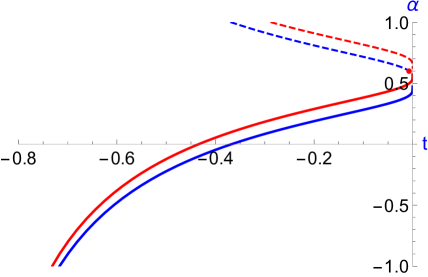
We consider stationary solution of Leray-like equation (8), and drop the variable in the velocity field. The expression in (33) is equivalent to (36) with linked to the couple () by the relation (29). As written in the text, any self-similar solution which satisfies (36) , with a given , has an amplitude proportional to a fixed coefficient which increases with respect to time as , with constant value during the pre (or post)-collapse. However expressions (28)-(29) mean that for a given value of time , and given (the asymptotic value at singular time) the stretching of the solution is different from the stretching of , except at singular time . More precisely one can say
- either that at time is the same as at time such that ,
- or else that is stretched at time as the solution (at the same time) associated to the exponent given by (29).
Fig. 4 displays the evolution of versus for (dashed lines) and (solid lines) for two values of the asymptotic exponent , the Sedov-Taylor value and the NS value. The solid curves are for larger than unity, they correspond to a solution with amplitude and width smaller than . They are interpreted as responsible for the peak observed in , see below. Dashed curves are for smaller than unity, namely for the dilated solution with amplitude and width larger than u(x,t,1).
IV.0.2 Link with experiments
We propose an interpretation of this discrepancy between the value of in (17) and the experimental one (20) by looking at the role of the dilation invariance of Euler (and NS) solutions.
Assuming, as done in this section, that a family of Euler-Leray solutions exist with a continuum of values, the signal recorded at a given place must reflect a large variety of exponent values , or equivalently . More precisely, for a given value, one expects that the behavior of the structures functions for the acceleration is given by (17) with given by (29), so that in average, one get
| (37) |
where means an average over values, is the exponent in (17) with replaced by the expression (29) , that gives
| (38) |
A rough estimate of the average (37) can be given by assuming that the values of contributing to this expression are those around a given which is to be deduced from the experimental results. To do that we identify the slope of the exponent in (38) with the experimental value . We get the relation . This result allows to conclude that if the main contributions to the striking peak observed in curves for large and small values come from Leray singularities, they are due to the small amplitudes solutions with
| (39) |
Let us now return to our previous analysis of Modane’s data presented in PC . There we made a statistical studies of the coupling between large acceleration and velocities values recorded at the same time, namely we didn’t look at the spatial autocorrelation of the acceleration contrary to what we do here for the study of (with the same data). In PC we got a very good agreement between the scaling predicted (with Sedov-Taylor-singularities) and those deduced by the record. We deduce that this study focused on the range of self-similar solutions with small values of , or amplitude of order unity,
| (40) |
In summary the role of the dilation invariance could amount to select bursts of different amplitude according to the statistical analysis performed, Sedov-Taylor exponents are detected from large amplitude bursts, larger than those which contribute to .
Another explanation of the discrepancy between experimental results and the values of predicted in (17) within the hypothesis of , could be that depends on . This possibility is not considered in this section, and as shown below it requires either that also depends on (not only via the dilation parameter), or that (42) is fulfilled. In that case one has to go beyond the frame of self-similar solutions, nevertheless one can infer from (29) that if the a solution at given value shifts to another value of before or after the formal blow-up time , the signal recorded by the probe should include this change of power law.
IV.0.3 Stationary solution of time dependent Leray equation (8)
The function depends on the reduced spatial variable , moreover it may depend on or not. If depends on , the Euler equation is equivalent to what we call the ”time dependent Leray” equation (8) for , which can also be written as
| (41) |
where the prime exponent is for the time derivative . If (or ) doesn’t depend on , (41) doesn’t depend on . But if one assumes the opposite, namely that and (or ) depend on , then a stationary solution of (41) exists only if
| (42) |
Acknowledgments
The authors are very grateful to Jean Ginibre for very useful discussions.
References
- (1) L. Euler, ”Principes généraux du mouvement des fluides”, Mémoires de l’Académie de Berlin (1757).
- (2) J. Leray, ”Essai sur le mouvement d’un fluide visqueux emplissant l’espace”, Acta Math. 63 (1934) p. 193 - 248.
- (3) Y. Pomeau, M. Le Berre and T. Lehner, C.R. Méc. Paris, 347 (2019) p. 342. in special issue dedicated to Pierre Coullet.; ArXiv:1806.04893v2.
- (4) B.E. Launder, D.B. ; Spalding, ”The numerical computation of turbulent flows”. Computer Methods in Applied Mechanics and Engineering, 3, (1974) p. 269- 289.
- (5) Y. Gagne, ’Etude expérimentale de l’intermittence et des singularités dans le plan complexe en turbulence développée, PhD thesis Université de Grenoble 1 (1987).
- (6) H. Kahalerras, Y. Malécot, Y. Gagne, and B. Castaing, Intermittency and Reynolds number, Phys. of Fluids 10 (1998) 910.
- (7) M. Bourgoin, C. Baudet, N. Mordant, T. Vandenberghe et al. , Investigation of the small-scale statistics of turbulence in the Modane S1MA wind tunnel , CEAS Aeronaut J., published online, July 2017. DOI 10.1007/s13272-017-0254-3
- (8) Y. Pomeau, ”Singularité dans l’évolution du fluide parfait”, C. R. Acad. Sci. Paris 321 (1995), p. 407 -411
- (9) C. Josserand, Y. Pomeau and S. Rica, Finite-time localized singularities as a mechanism for turbulent dissipation, in preparation.
- (10) Y. Pomeau, M. Le Berre, Blowing-up solutions of the axisymmetric Euler equations for an incompressible fluid, arXiv:1901.09426.
- (11) S. Chapman and T. G. Cowling, The Mathematical Theory of Non-Uniform Gases (Cambridge University Press, Cambridge, UK, 1970), 3rd ed. ; P. Résibois and M. de Leener, Classical Kinetic Theory of Fluids (John Wiley and Sons, New York, 1977). Notice however that, because of the long tails of time correlations of dense fluids, the Burnett coefficients do not exist in dense fluids similarly as the usual transport coefficients do not exist in 2D dense fluids. Burnett transport coefficients exist in the low density limit only when Boltzmann equation applies.
- (12) B. A. Toms ”Observation on the flow of linear polymer solutions through straight tubes at large Reynolds numbers” Proceedings of the First International Congress of rheology Amsterdam, Vol. II, p.135 - 141 (North Holland 1949).