Branched Josephson junctions:
Current carrying solitons in external magnetic fields

Abstract

We consider branched Josephson junction created by planar superconductors connected to each other through the Y-junction insulator. Assuming that the structure interacts with the external constant magnetic field, we study static sine-Gordon solitons in such system by modeling them in terms of the stationary sine-Gordon equation on metric graph. Exact analytical solutions of the problem are obtained and their stability is analyzed.

1 Introduction

Low dimensional nanoscale materials are the basic structures for many electronic devices. Optimization of their electronic properties and effective functioning of such devices require tuning the material properties and revealing most appropriate device architecture. This concerns also superconducting structures such as Josephson junctions. Remarkable feature of Josephson junctions is the fact that the phase difference at the junction is described in terms of the sine-Gordon equation (see, e.g. [1]-[7]). This makes them powerful testing ground for experimental realization of sine-Gordon solitons [9]-[15]. So far, different models have been proposed for the study of static and traveling solitons using Josephson junctions [16] -[22].

In this paper we address the problem of static solitons in branched Josephson junction containing planar superconductors connected to each other via the branched insulators having the shape of Y-junction. The system is considered as interacting with constant external magnetic field. The phase differences on each branch of such structure is described in terms of the stationary sine-Gordon equation on metric graphs. Earlier, in the Ref.[47] we considered a version of such system for the case of absence of current carrying states. Unlike to that case, in the present study, including current leads to completely different vertex boundary conditions, and hence, to different solutions than those obtained in [47]. Provided certain constraints given in terms of the system parameters, we obtain exact analytical solutions of the stationary sine-Gordon equation on metric graphs, modeling static solitons in branched Josephson junction. Motivation for the study of such model comes from several practically important problems, such as superconducting quantum interference devices (SQUID in networks), superconducting qubits in networks, as well as granular superconductors. Among others, most attractive practical application could be experimental realization of sine-Gordon solitons in networks. We note that the soliton dynamics in networks is becoming one of the hot topics in nonlinear and mathematical physics [26, 27, 34]- [53]. Refs.[26, 27] considered for the first time the sine-Gordon equation on branched domain for modeling Josephson junction at tricrystal surfaces. Integrable sine-Gordon equation on metric graphs is studied in [39, 44, 47]. Linear and nonlinear systems of PDE on metric graphs are considered in [48, 49, 50].
Among different realizations of Josephson junctions those having the discrete and branched structure is of special importance, as it allows to study soliton dynamics in discrete systems and networks. The early treatment of superconductor networks consisting of Josephson junctions meeting at one point dates back to [24]. An interesting realization of Josephson junction networks at tricrystal boundaries was discussed earlier in [25], which inspired later detailed study of the problem using the sine-Gordon equation on networks in [26, 27]. Some versions of Josephson junction networks containing chain of the linear superconductors connected via the point-like insulators, have been studied on the basis of discrete sine-Gordon model [28]-[33]. Unlike the previously discussed versions of Josephson junction networks, our model is simple from the viewpoint of experimental realization and can be studied .
The paper is organized as follows. In the next section we give a formulation of the problem in terms of the sine-Gordon equation on metric graphs. Section III presents the derivation of exact analytical solutions for special cases and their stability analysis. Finally, Section IV presents some concluding remarks.

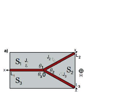
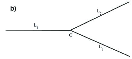
Figure 1: (Color online) (a) Branched Josephson Y-junction in a constant magnetic field, $H$. Red lines imply normal metal or insulator. $J_{1},J_{2}$ and $J_{3}$ are the Josephson currents flowing through each branch of the junction. b) Basic star graph. $L_{j}$ is the length of the $j$th branch of the graph($j=1,2,3$).

2 Modeling of branched Josephson junction in terms of metric graph

Consider the structure presented in Fig. 1a, which represents a Josephson junction consisting of three planar superconductors connected to each other via the branched insulator in the form of Y-junction. The whole system is assumed to interact with external constant magnetic field, $H$ which is perpendicular to the plane of superconductors. Such structure can be considered as the branched version of the Josephson junction considered in the Refs.[20, 21]. The structure can be modeled in terms of metric star graph having three branches, i.e., simple Y-junction( see, Fig. 1b). For each bond of the star graph a coordinate $x_{j}$ is assigned. The origin of coordinates at the vertex, 0 and for bonds we put $x_{j}\in[0;L_{j}]$. Then on can use shorthand notation $\phi_{j}(x)$ for $\phi_{j}(x_{j})$, where $x$ is the coordinate on the bond $j$ to which the component $\phi_{j}$ refers. The phase difference on each branch $\phi_{j}$, is described in terms of the stationary sine-Gordon equation on metric star graph [47]:

$$\frac{d^{2}}{dx^{2}}\phi_{j}=\frac{1}{\lambda_{j}^{2}}\sin(\phi_{j}),\,0<x<L_{j},$$ (1)

where $j=1,2,3$ is the bond (branch) number and the origin of coordinates is assumed at the branching point, $O$. To solve this equation, one needs to impose boundary conditions at the branching point, $O$. Such boundary conditions can be derived from the physical properties of the structure presented in Fig. 1a. Computing, at the branching point, the phase differences, $\phi_{1}=\theta_{1}-\theta_{3}$, $\phi_{2}=\theta_{1}-\theta_{2}$, $\phi_{3}=\theta_{2}-\theta_{3}$, where $\theta_{1,2,3}$ are the phases on each superconductor, one can obtain first set of the vertex boundary conditions given by

$$\phi_{1}|_{x=0}-\phi_{2}|_{x=0}-\phi_{3}|_{x=0}=0.$$ (2)

In the following we will use the system of units $\hbar=c=2\pi d=e=1$, where $d$ is equal to twice the penetration depth (for identical superconductors) plus the insulator (or normal metal) thickness [54]. In such units, e.g., for $d=1mm$ $J_{j}=1$ is equal to $\approx 7.64nA$, and for the magnetic field $H=1$ implies that $H\approx 1.22\mu A/m$, etc.

Then the local magnetic field in terms of $\phi_{j}$ can be written as

$$h_{j}(x)=\frac{\partial\phi_{j}}{\partial x},$$ (3)

where we have scaled the local magnetic field over $\pi$ (i.e. $\frac{h_{j}(x)}{\pi}\to h_{j}(x)$). The current density on each branch of the junction is given as [21, 54, 55]

$$j_{j}(x)=\frac{1}{4\lambda_{j}^{2}}\sin\phi_{j}(x).$$ (4)

Integrating Eq. (4) over the each bond and using Eq. (1) we can find the current on each bond as [54]

$$J_{j}=\frac{1}{4}\left(\left.\frac{d\phi_{j}}{dx}\right|_{x=L_{j}}-\left.\frac{d\phi_{j}}{dx}\right|_{x=0}\right).$$ (5)

Using continuity of the local magnetic field $h_{j}(x)$ at the branching point ($h_{1}(0)=h_{2}(0)=h_{3}(0)$) we get the second set of vertex boundary conditions:

$$\left.\frac{d\phi_{1}}{dx}\right|_{x=0}=\left.\frac{d\phi_{2}}{dx}\right|_{x=0}=\left.\frac{d\phi_{3}}{dx}\right|_{x=0}.$$ (6)

For complete formulation of the problem, one needs also to impose boundary conditions at the end of each branch. This can be done by writing explicitly the value of local magnetic field in terms of external and intrinsic magnetic field. These latter are supposed to be induced by Josephson current on each branch. Denoting this magnetic field on each branch by $H_{Jj}$ ($j=1,2,3$) we have the following Neumann type boundary conditions at the end of each branch:

$$\left.\frac{d\phi_{1}}{dx}\right|_{x=L_{1}}=H+H_{J1},$$

$$\left.\frac{d\phi_{2}}{dx}\right|_{x=L_{2}}=H-H_{J2},$$

$$\left.\frac{d\phi_{3}}{dx}\right|_{x=L_{3}}=H-H_{J3}.$$ (7)

Writing the same expression at the branching point, one can derive explicit relation expressing the external magnetic field, $H$ in terms of the derivatives of phase differences:

$$H=\frac{1}{4}\sum_{j=1}^{3}\left.\frac{d\phi_{j}}{dx}\right|_{x=L_{j}}+\frac{1}{4}\left.\frac{d\phi_{1}}{dx}\right|_{x=0}.$$ (8)

The problem given by Eqs.(1), (2), (6) and (7) completely determines the problem of sine-Gordon equation on metric star graph, which is the model for the static solitons in branched Josephson junction presented in Fig.1a.

Exact solutions of Eq.(1) for the boundary conditions providing the absence of current-carrying states ($J_{j}=0$), have been obtained in [47], where the stability of such solutions also was analyzed. Here we consider current carrying states ($J_{j}\neq 0$) in the branched Josephson junction, which are described by different boundary conditions.

3 Static solitons and their stability

The problem given by Eqs. (1), (2), (6) and (7) have different types of solutions. However, only the stable solutions of this problem can be considered as the physical ones. These latter describe the phase difference in branched Josephson junction in Fig.1a. Therefore, following the Refs.[20, 21], we provide prescription for stability analysis for the solutions of Eq.(1). Starting point for such analysis is the Gibbs free-energy functional which can be written as [20, 21]

$$\Omega_{G}={\sum}_{j=1}^{3}\Omega_{G}^{(j)}\left[\phi_{j},\frac{d\phi_{j}}{dx};H,H_{J1},H_{J2},H_{J3}\right],$$ (9)

where $\Omega_{G}^{(j)}$ is the Gibbs free energy functional on each bond (see the Ref.[23] for details of the derivation of $\Omega_{G}$), which is given by

$$\Omega_{G}^{(j)}\left[\phi_{j},\frac{d\phi_{j}}{dx};H,H_{J1},H_{J2},H_{J3}\right]=2H^{2}L_{j}-$$

$$-\left(H\pm H_{Jj}\right)\phi_{j}(L_{j})+$$

$$+\left(H-H_{J1}+H_{J2}+H_{J3}\right)\phi_{j}(0)+$$

$$+\int\limits_{0}^{L_{j}}\left[\frac{1}{\lambda_{j}^{2}}\left(1-\cos\phi_{j}(x)\right)+\frac{1}{2}\left(\frac{d\phi_{j}(x)}{dx}\right)^{2}\right]dx,$$ (10)

where we take the ”+” sign for $j=1$, and ”-” sign for other cases. Eq.(1) together with the boundary conditions (2), (6), (7) follows from the condition

$$\delta\Omega_{G}=0.$$ (11)

Criterion for the stability of the solution of problem given by Eqs.(1), (2), (6) and (7), can be obtained from the second variation of $\Omega_{G},$ i.e., from

$$\Omega_{G}=0,$$

which leads to the following Sturm-Liouville problem [20, 21, 47]:

$$-\frac{d^{2}\psi_{j}}{dx^{2}}+\frac{1}{\lambda_{j}^{2}}\cos\phi_{j}(x)\psi_{j}=\mu\psi_{j},\,0<x<L_{j},$$

$$\psi_{1}|_{x=0}-\psi_{2}|_{x=0}-\psi_{3}|_{x=0}=0,$$

$$\left.\frac{d\psi_{1}}{dx}\right|_{x=0}=\left.\frac{d\psi_{2}}{dx}\right|_{x=0}=\left.\frac{d\psi_{3}}{dx}\right|_{x=0},$$

$$\left.\frac{d\psi_{j}}{dx}\right|_{x=L_{j}}=0,\,j=1,2,3,$$ (12)

where $\psi_{j}=\delta\phi_{j},\;\;j=1,2,3.$ In terms of the lowest eigenvalue, $\mu_{0}$, the criterion for stability of the solution can be formulated as follows. If $\mu_{0}<0,$ the solution $\phi_{j}(x)$ corresponds to a saddle point of Eq.(9) which implies that the solution is absolutely unstable and unphysical. Stable (physical) solutions correspond to the case, when $\mu_{0}>0,$ ($\delta^{2}\Omega_{G}>0$). The boundaries of the stability regions for these solutions is determined by the condition $\mu_{0}=0$ ($\delta^{2}\Omega_{G}=0$), that leads to the following Sturm-Liouville problem:

$$-\frac{d^{2}\bar{\psi}_{j}}{dx^{2}}+\frac{1}{\lambda_{j}^{2}}\cos\phi_{j}(x)\bar{\psi}_{j}=0,\,0<x<L_{j},$$ (13)

$$\bar{\psi}_{1}|_{x=0}-\bar{\psi}_{2}|_{x=0}-\bar{\psi}_{3}|_{x=0}=0,$$ (14)

$$\left.\frac{d\bar{\psi}_{1}}{dx}\right|_{x=0}=\left.\frac{d\bar{\psi}_{2}}{dx}\right|_{x=0}=\left.\frac{d\bar{\psi}_{3}}{dx}\right|_{x=0},$$ (15)

$$\left.\frac{d\bar{\psi}_{j}}{dx}\right|_{x=L_{j}}=0,\,j=1,2,3.$$ (16)

Using Eqs.(13)-(16), one can explicitly find the stability boundary for each type of solution of the problem given by Eqs. (1), (2), (6) and (7).

General solution of Eq.(1) can be obtained from the following first integral [20, 21]:

$$\frac{1}{2}\left[\frac{d\phi_{j}}{dx}\right]^{2}+\cos\phi_{j}=C_{j},\;\;-1\leq C_{j}<\infty,$$ (17)

with $C_{j}$ being the integration constant. Depending on the value of $C_{j}$ this general solution can be determined as type I and II. Namely, for $C_{j}\in[-1,1)$ we have solution of type I, while solution of type II corresponds to the values, $C_{j}\in[1,\infty)$. Both solutions for $H\neq 0,$ and $J_{j}=0$ have been found in [47] where it was shown that only the special case of the solution of type II is stable. Following the Refs. [20, 21], instead of $C_{j}$ we introduce new parametrization constant, $k_{j}$, which is defined, for the solution of type I as

$$k_{j}^{2}\equiv\frac{1+C_{j}}{2},\;-1<k_{j}<1,$$

and

$$k_{j}^{2}\equiv\frac{2}{1+C_{j}},\;-1<k_{j}<1,$$

for solution of type II. General (type I) solution of Eq.(1) can be written as [20, 21, 47]

$$\phi_{j}(x)=(2n_{j}+1)\pi+2\arcsin\left\{k_{j}sn\left[\frac{x-x_{0j}}{\lambda_{j}},k_{j}\right]\right\}$$ (18)

where $sn$ is Jacobi elliptic function [56], and $x_{0j}$ are integration constants which obey the constraints given by the following inequality:

$$-\lambda_{j}K(k_{j})<x_{0j}<\lambda_{j}K(k_{j}),\;\;j=1,2,3.$$

Solution given by Eq. (18) fulfils the vertex boundary conditions given by Eqs. (2), (6) and (7), i.e., becomes exact analytical solution of the problem given by Eqs. (1), (2), (6) and (7), provided the following constraints hold true:

$$\lambda_{1}=\lambda_{2}=\lambda_{3}=\lambda,\,k_{1}=k_{2}=k_{3}=k,$$

$$-\frac{x_{01}}{\lambda_{1}}=\frac{x_{02}}{\lambda_{2}}=\frac{x_{03}}{\lambda_{3}}=x_{0}.$$ (19)

$$n_{1}=n_{2}+n_{3}.$$ (20)

The solution (18) can be stable only for those values of $k$ which belong to the interval $[k_{c},1)$ ($k_{c}sn[x_{0},k_{c}]=\frac{1}{2}$). Therefore in the following, in analogy with that in the Ref.[21], we compute the physical characteristics of the system at $k=k_{c}(x_{0})$ which correspond to its values at the stability border. Using the relation

$$\frac{d\phi_{j}(x)}{dx}=-\frac{2k}{\lambda}cn\left[\frac{x}{\lambda}\pm x_{0},k\right],$$ (21)

and Eq. (7), when $j=1$ we take $+$ sign , when $j=2,3$ we take $-$ sign, the stability border for the current-carrying states can be written as:

$$J_{j}^{(c)}=-\frac{k_{c}}{2\lambda}\left(cn\left[\frac{L_{j}}{\lambda}\pm x_{0},k_{c}\right]-cn\left[x_{0},k_{c}\right]\right),$$ (22)

$$H^{(c)}=-\frac{k_{c}}{2\lambda}\left(\sum_{j=1}^{3}cn\left[\frac{L_{j}}{\lambda}\pm x_{0},k_{c}\right]+cn\left[x_{0},k_{c}\right]\right).$$ (23)

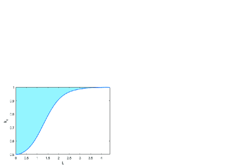
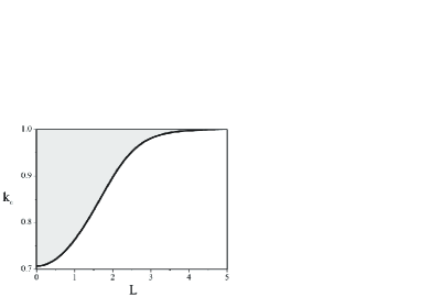
Figure 2: (Color online) Upper panel: The dependence of the stability border, $k_{c}=k_{c}(L)$ on the branch length,(solid line) for the branched Josephson junction. Colored area corresponds to the stability area. Lower panel: similar plot in the linear (unbranched) case from the Ref.[21].

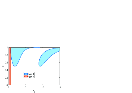
Figure 3: (Color online) The stability region (colored) of $\phi$ in the parametric plane. Branch lengthes are $L_{1}=1,L_{2}=2,L_{3}=3$.

Fig.2 presents plot of $k_{c}$ as a function of the parameter, $L$ determined from $L_{1}=L,L_{2}=2L,L_{3}=3L$. The left (colored) area of each plot corresponds to the stability region. Lower panel in this figure presents corresponding plot for linear case from the Ref.[21]. Since $k_{c}$ appears as the value of $k$ at which the Sturm-Liouville (stability) problem has zero ($\mu_{0}=0$) eigenvalue, it is important to check, at which values of $x_{0}$ this is possible. Fig. 3 presents plot of $k_{c}$ as a function of $x_{0}$, i.e., the stability region of $\phi$ in the parametric plane. Colored area corresponds to the stability region.
The solution of type II can be treated similarly to that of type I, by considering two cases. The case $H>0,\,J_{j}=0$ has been studied in detail in the Ref. [47]. Therefore we drop this part. Here we will focus on the case $H>0,\,J_{j}>0$. General (type II) solution for this case can be written as

$$\phi_{j}(x)=\pi(2n_{j}+1)+2am\left(\frac{x-x_{0j}}{\lambda_{j}k_{j}},k_{j}\right).$$ (24)

Fulfilling the boundary conditions given by Eqs. (2) and (6) leads to the constraints in Eqs.(19) and (20). Stable solutions and the border between stability and unstable regions can be determined similarly to that for solution type I.

From Eqs. (5) and (8) we get the expressions for current and magnetic field

$$J_{j}=\frac{1}{2\lambda k}\left(dn\left[\frac{L_{j}}{\lambda k}\pm x_{0},k\right]-dn\left[x_{0},k\right]\right),$$ (25)

$$H=\frac{1}{2\lambda k}\left(\sum_{j=1}^{3}dn\left[\frac{L_{j}}{\lambda k}\pm x_{0},k\right]+dn\left[x_{0},k\right]\right),$$ (26)

$$x_{0}\in[0;x_{0,c}].$$ (27)

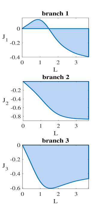
Figure 4: (Color online) The dependence $J_{c}=J_{c}(L)$ for $H=0$ (solid line). The stability region is colored, parameters are the same as in Fig.2.

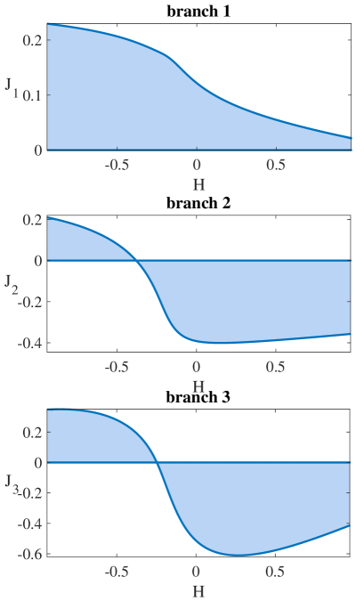
Figure 5: (Color online) The stability region (colored) of $\phi_{j}$ in the physical plane $(J,H)$ for type 1 solutions and the same parameters as in Fig.3.

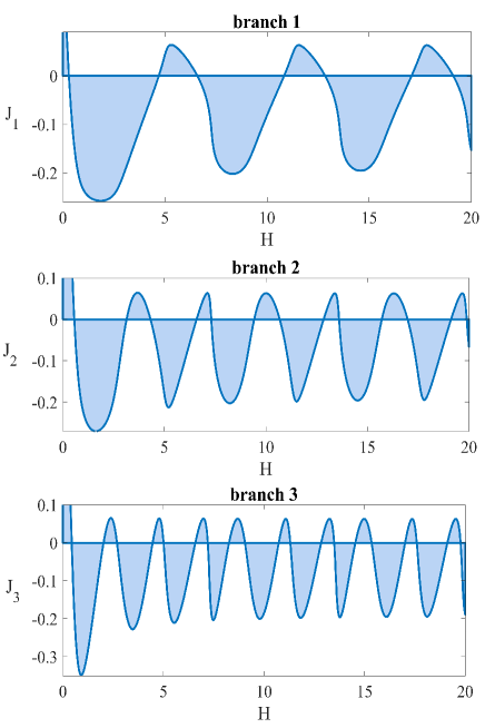
Figure 6: (Color online) The stability region (colored) of $\phi_{j}$ in the physical plane $(J,H)$ for type 2 solutions and the same parameters as in Fig.3.

In Fig. 4, the dependence of the current on the branch length, $L_{j}$ is plotted. Colored (lower) parts corresponds to the the stability area. Figs. 5 and 6 present the plots of the current, $J_{j}$ as a function of the magnetic field for type 1 and type 2, respectively. The colored area in each plot corresponds to the stability region, i.e, presents the stability region of $\phi_{j}$ in the physical plane $(J,H)$.

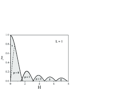
Figure 7: The stability region of $\phi_{j}$ in the physical plane $(J,H)$ for linear (unbranched) Josephson junction from Ref.[21].

It is meaningful to compare the above results with those for their linear (unbranched)counterpart considered in the Ref.[21]. Comparing dependence of $k_{c}$ on $L$ presented in Fig.2, with the corresponding plot from for linear case, one can conclude that they are very close to each other. However, differences between linear and branched cases appear in the plots of $J_{j}(L)$ and $J_{j}(H)$ presented in Figs. 3 - 6, respectively. Comparing $J_{j}(H)$ in Figs. 5 and 6 for branched Josephson junction with corresponding plot in Fig.7 for linear case, one can find considerable difference both in the shape and area of the stability region. In particular, for branched case the total area of the stability region is much larger than that for linear counterpart. Moreover, due to the fact that branched system has more parameters, one can make it tunable with respect to playing with these parameters. Especially, this concerns the case of more complicated branching architecture, e.g., junction with tree-like branching presented in Fig. 8. Static solitons in this structure can be modeled in terms of the sine-Gordon equation with the boundary conditions given on metric tree graph.

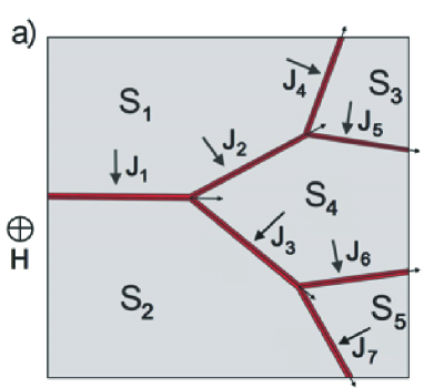
Figure 8: (Color online) Tree-like branched Josephson junction.

4 Conclusions

We have studied the current carrying states in branched Josephson junction interacting with the external magnetic field. The structure is assumed to be constructed, from three planar superconductors connected to each other via the insulating (or normal metal) Y-junction. The system is modeled in terms of the stationary sine-Gordon equation on the metric star graph, whose solutions describe the phase difference between the superconductors on the each branch of the junction. The boundary conditions for the sine-Gordon equation at the branching point are derived from the relation between current, local and external magnetic fields. Exact analytical solutions of sine-Gordon equation fulfilling such boundary conditions are obtained. The stability regions for these solutions are determined in terms of the integration constant using the Gibbs free energy functional based (variational) approach. Physical observable values of the current described in terms of the stable solutions are derived explicitly as a function of the magnetic field. Finally, we note that although we considered very simple branching having the form of Y-junction, the approach we used can be directly extended for modeling static solitons in more general branching architectures of the junction, such as tree, loop, triangle, etc. This can be done similarly to that in [47], where sine-Gordon equation on metric graphs is solved for $J_{j}=0$. Considering such complicated branching architectures is of importance from the viewpoint of the device tuning and optimization in such problems as SQUID, superconducting qubit, cold atom trapping and Majorana wire networks.

- [1] \NameJosephson B. D. \REVIEWRev. Mod. Phys.361964216.
- [2] \NameJosephson B. D. \REVIEWRev. Mod. Phys.461974251.
- [3] \NameBarone A. Paterno G. \BookPhysics and Applications of the Josephson Effect \PublWiley, New York \Year1982
- [4] \NameLikharev K. K. \BookDynamics of Josephson Junctions and Circuits \PublCRC Press \Year1986
- [5] \NameMcCann J. \BookJosephson Junction and Superconductivity Research \PublNova Science Publishers \Year2007
- [6] \BookJosephson Junctions: History, Devices, and Applications \Editor Wolf E. L., Arnold G. B., Gurvitch M. A., Zasadzinski J. F. \PublPan Stanford Publishing \Year2017
- [7] \NameAskerzade I., Bozbey A., Canturk M. \BookModern Aspects of Josephson Dynamics and Superconductivity Electronics \PublSpringer \Year2017
- [8] \BookThe sine-Gordon model and its applications : from Pendula and Josephson junctions to gravity and high-energy Physics \EditorCuevas-Maraver J., Kevrekidis P.G. Williams F. \PublSpringer International Publishing \Year2014
- [9] \NameAblowitz M.J., Segur H. \BookSolitons and the Inverse Scattering Transform \PublSIAM, Philadelphia \Year1981
- [10] \NameRajaraman R. \BookSolitons and Instantons \PublElsevier, Amsterdam \Year1982
- [11] \NameDrazin P.G., Johnson R.S. \BookSolitons: an introduction \PublCambridge University Press \Year1989
- [12] \NameAblowitz M.J. Clarkson P.A. \BookSolitons, Nonlinear Evolution Equations and Inverse Scattering \PublCambridge University Press \Year1999
- [13] \NameDauxois T., Peyrard M. \BookPhysics of Solitons \PublCambridge University Press, Cambridge \Year2006
- [14] \NameScott A. C. \BookNonlinear science, emergence and dynamics of coherent structures \PublOxford University Press \Year2003
- [15] \NameBraun O., Kivshar Yu. \BookThe Frenkel-Kontorov Model \PublSpringer \Year2004
- [16] \NameMalomed B. A. \REVIEWPhys. Rev. B3919898018(R).
- [17] \NameUstinov A. V., Doderer T. Huebener R. P. textitet.al \REVIEWPhys. Rev. Lett6919921815.
- [18] \NameHermon Z., Ben-Jacob E., Schoen G. \REVIEWPhys. Rev. B5419961234.
- [19] \NameCarapella G., Costabile G., Sabatino P. \REVIEWPhys. Rev. B58199815094.
- [20] \NameKuplevakhsky S. V. Glukhov A. M. \REVIEWPhys. Rev. B732006024513.
- [21] \NameKuplevakhsky S. V. Glukhov A. M. \REVIEWPhys. Rev. B762007174515.
- [22] \NameFedorov K. G., Fistul M. V., Ustinov A. V. \REVIEWPhys. Rev. B842011014526.
- [23] \NameKuplevakhsky S. V. \REVIEWLow Temp. Phys.302004646.
- [24] \NameNakajima K., Onodera Y., Ogawa Y. \REVIEWJ. Appl. Phys.4919782958.
- [25] \NameKogan V., Clem J., Kirtley J. \REVIEWPhys. Rev. B6120009122.
- [26] \NameSusanto H.,van Gils S., Doelman A., Derks G. \REVIEWPhysica C4082004579.
- [27] \NameSusanto H.,van Gils S., Doelman A., Derks G. \REVIEWPhys. Rev. B692004212503.
- [28] \NameDe Luca R., Romeo F. \REVIEWPhys. Rev. B662002024509.
- [29] \NameGiuliano D. Sodano P. \REVIEWEurphys.Lett.88200917012.
- [30] \NameGiuliano D. Sodano P. \REVIEWNucl. Phys. B8112009(FS) 395.
- [31] \NameGiuliano D. Sodano P. \REVIEWNucl. Phys. B8372010(FS) 153.
- [32] \NameGiuliano D. Sodano P. \REVIEWEPL103201357006.
- [33] \NameOvchinnikov Yu. N., Kresin V. Z. \REVIEWPhys. Rev. B882013214504.
- [34] \NameSobirov Z., Matrasulov D., Sabirov K., Sawada S., Nakamura K. \REVIEWPhys. Rev. E812010066602.
- [35] \NameZ. Sobirov, D. Matrasulov, S. Sawada, and K. Nakamura \REVIEWPhys.Rev.E842011026609.
- [36] \NameAdami R., Cacciapuoti C., Finco D., Noja D. \REVIEWRev.Math.Phys2320114.
- [37] \NameSabirov K.K., Sobirov Z.A., Babajanov D., Matrasulov D.U. \REVIEWPhys.Lett. A3772013860.
- [38] \NameNoja D. \REVIEWPhilos. Trans. R. Soc. A372201420130002.
- [39] \NameCaputo J.-G., Dutykh D. \REVIEWPhys. Rev. E902014022912.
- [40] \NameUecker H., Grieser D., Sobirov Z., Babajanov D. Matrasulov D. \REVIEWPhys. Rev. E912015023209.
- [41] \NameNoja D., Pelinovsky D., Shaikhova G. \REVIEWNonlinearity2820152343.
- [42] \Name R.Adami, C.Cacciapuoti, D.Noja \REVIEWJ. Diff. Eq.26020167397.
- [43] \NameCaudrelier V. \REVIEWComm. Math. Phys.3382015893.
- [44] \NameSobirov Z., Babajanov D., Matrasulov D., Nakamura K., Uecker H. \REVIEWEPL115201650002.
- [45] \NameAdami R., Serra E., Tilli P. \REVIEWCommun. Math. Phys.3522017387.
- [46] \NameKairzhan A., Pelinovsky D.E. \REVIEWJ. Phys. A: Math. Theor.512018095203.
- [47] \NameSabirov K.K., Rakhmanov S., Matrasulov D. Susanto H. \REVIEWPhys.Lett. A38220181092.
- [48] \NameBolte J. and Harrison J. \REVIEWJ. Phys. A: Math. Gen.362003L433.
- [49] \NameSabirov K.K., Yusupov J., Jumanazarov D., Matrasulov D. \REVIEWPhys.Lett. A38220182856.
- [50] \NameSabirov K.K., Babajanov D.B., Matrasulov D.U. and Kevrekidis P.G. \REVIEWJ. Phys. A: Math. Theor.512018435203.
- [51] \NameJ. R. Yusupov, K. K. Sabirov, M. Ehrhardt and D. U. Matrasulov \REVIEWPhys. Lett. A38320192382.
- [52] \NameBabajanov D., Matyoqubov H. and Matrasulov D. \REVIEWJ. Chem. Phys.1492018164908.
- [53] \Name Yusupov J. R., Sabirov K. K., Ehrhardt M. Matrasulov D. U. \REVIEWPhys. Rev. E1002019032204.
- [54] \Name Owen C. S, Scalapino D. J. \REVIEWPhys. Rev.1641967538.
- [55] \NameG. F. Zharkov \REVIEWSov. Phys. JETP 4819701107.
- [56] \NameAbramowitz M. Stegun I. A. \BookHandbook of Mathematical Functions \PublDover, New York \Year1965
- [57] \NameBanerjee S., Fransson J., Black-Schaffer A. M., et.al \REVIEWPhys. Rev. B932016134502.
- [58] \Name Widom A., Badjou S. \REVIEWPhys. Rev. B3719887915(R).
- [59] \NamePeterson R. L., Ekin J. W. \REVIEWPhys. Rev. B3719889848(R).
- [60] \NameR. S. Fishman \REVIEWPhys. Rev.B3919897228.