Choked accretion onto a Schwarzschild black hole:
A hydrodynamical jet-launching mechanism

Abstract

We present a novel, relativistic accretion model for accretion onto a Schwarzschild black hole. This consists of a purely hydrodynamical mechanism in which, by breaking spherical symmetry, a radially accreting flow transitions into an inflow-outflow configuration. The spherical symmetry is broken by considering that the accreted material is more concentrated on an equatorial belt, leaving the polar regions relatively under-dense. What we have found is a flux-limited accretion regime in which, for a sufficiently large accretion rate, the incoming material chokes at a gravitational bottleneck and the excess flux is redirected by the density gradient as a bipolar outflow. The threshold value at which the accreting material chokes is of the order of the mass accretion rate found in the spherically symmetric case studied by Bondi and Michel. We describe the choked accretion mechanism first in terms of a general relativistic, analytic toy model based on the assumption of an ultrarelativistic stiff fluid. We then relax this approximation and, by means of numerical simulations, show that this mechanism can operate also for general polytropic fluids. Interestingly, the qualitative inflow-outflow morphology obtained appears as a generic result of the proposed symmetry break, across analytic and numeric results covering both the Newtonian and relativistic regimes. The qualitative change in the resulting steady state flow configuration appears even for a very small equatorial to polar density contrast ($\sim$0.1%) in the accretion profile. Finally, we discuss the applicability of this model as a jet-launching mechanism in different astrophysical settings.

1 Introduction

Astrophysical jets are found in vastly different scenarios: from the parsec scales of the H-H objects associated with young stellar systems (Hartigan, 2009), to the megaparsec scales of the radio lobes that accompany some radio galaxies and other Active Galactic Nuclei (AGN) (Beckmann & Shrader, 2012). They are also inferred in connection with high energy phenomena such as long Gamma Ray Bursts (GRBs) following the collapse of a massive star (Woosley & Bloom, 2006), jetted emission associated with micro-quasars in some X-ray binaries (Mirabel & Rodríguez, 1994), X-ray flares after a stellar tidal disruption event (Burrows et al., 2011), and short GRBs accompanying the kilonova explosion after the merger of two neutron stars (Abbott et al., 2017).

In recent decades, substantial progress has been made in understanding different aspects of astrophysical jets, particularly in relation to their acceleration and collimation (see e.g. Qian et al., 2018; Liska et al., 2019). However, open questions remain concerning the process of launching the jet in the first place, as well as the details connecting the accreted and ejected flows (Romero et al., 2017).

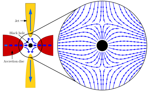
Figure 1: Schematic representation of the astrophysical setting under study: the inner region of an accretion disk-jet system around a central black hole. The analytic solution presented in this work constitutes a toy model of the inner engine behind a jet-launching process in which, through the action of hydrodynamical forces only, an accretion flow can be transformed into an inflow-outflow bipolar structure. Subsequent numerical simulations relaxing the assumptions included in the analytic solution, validate and extend the qualitative aspects of the solution found to more general cases. The blue arrows show schematically the streamlines of the resulting flow.

Several mechanisms have been proposed to address these issues. The most widely accepted ones are the mechanisms introduced by Blandford & Payne (1982) (BP) and Blandford & Znajek (1977) (BZ). The BP mechanism consists on the extraction of energy and angular momentum from an accretion disk, via a magneto-centrifugal process. The main ingredient is a global, poloidal magnetic field threading an accretion disk that rotates with Keplerian velocity. This mechanism is mostly used to explain the origin of jets in AGNs (e.g. Hawley et al., 2015; Blandford et al., 2019) and in YSOs (e.g. Ouyed et al., 2003; Pudritz et al., 2007; Fendt, 2018). On the other hand, the BZ mechanism shows an efficient way of extracting rotational energy from the spin of a Kerr black hole, provided a sufficiently strong magnetic field threads its event horizon. This mechanism has been used to explain the jets associated to GRBs (Lloyd-Ronning et al., 2019; Zhong et al., 2019) and radio jets in AGNs (Komissarov et al., 2007). Both mechanisms have been successfully tested under broad physical conditions using general relativistic, magneto-hydrodynamic simulations (e.g. Semenov et al., 2004; McKinney, 2006; Qian et al., 2018; Liska et al., 2019).

On the other hand, a purely hydrodynamical mechanism has been proposed by Hernandez et al. (2014) in which an axisymmetric, polar density gradient is responsible for deflecting part of the material accreting from an equatorially over-dense inflow and redirecting it along a bipolar outflow. The main advantage of this jet-launching mechanism is that for it to work, one does not need to invoke the presence of magnetic fields that might lack the necessary strength or geometry in some systems (Hawley et al., 2015), or processes taking place in the vicinity of a rotating event horizon and that, thus, can only account for jets associated with systems having a Kerr black hole as central accretor.

In this work, we revisit the jet-launching model of Hernandez et al. (2014) and study it in the general relativistic regime of an accreting, non-rotating black hole (Schwarzschild spacetime). Based on the general solution derived by Petrich, Shapiro, & Teukolsky (1988) for a relativistic potential flow with a stiff equation of state, we construct an analytic model corresponding to an inflow-outflow configuration around a Schwarzschild black hole. We propose that this analytic solution can be used as a toy model for the inner engine of a jet-launching system.

The physical setting of this model is shown schematically in Figure 1, and consists of the innermost region of an accretion disk-jet system around a central black hole. Specifically, we will confine our study to a finite, spherical region of radius $\mathcal{R}$ with the black hole at its center. We will refer to the surface of this domain as the injection sphere and consider it as the outer boundary of this system. Moreover, for the analytic model presented, in addition to considering a perfect fluid described by a stiff equation of state, we will assume stationarity, axisymmetry, and an irrotational flow, i.e. we consider that the gas entering the injection sphere from the inner edge of an accretion disk has lost all of its angular momentum through some kind of viscous dissipation mechanism (e.g Shakura & Sunyaev, 1973; Balbus & Hawley, 1991).

Even though for constructing the present model we do not include explicitly fluid rotation, it is important to remark that we have accounted for it indirectly by assuming that the flow configuration has a well defined symmetry axis, possibly as an inherited property of a rotation axis at larger scales. Furthermore, our assumption of a density anisotropy with the equatorial region having a higher density than the poles is a natural consequence of fluid rotation.

On the other hand, demanding a regular solution across the black hole event horizon implies that, for the present model with an ultrarelativistic stiff fluid, the total mass accretion rate onto the central black hole is fixed at a specific value (Petrich et al., 1988). This value corresponds closely to that found in the spherically symmetric case discussed by Michel (1972) for a Schwarzschild spacetime and by Bondi (1952) in the non-relativistic regime.

This important characteristic of the analytic model implies that the mass flux onto the central black hole is limited by a fixed value, and that any additional mass flux crossing the injection sphere has to be redirected and ejected from the system. In the present case, we show that the assumed anisotropic density field at the injection sphere translates into the bipolar outflow shown in Figure 1. Given that the incoming mass accretion rate is choking at a fixed value, we refer to this ejection mechanism as choked accretion.

With the aim of studying this accretion scenario under more general conditions, we also present the results of numerical simulations performed with the free GNU General Public License hydrodynamics code aztekas (Olvera & Mendoza, 2008; Aguayo-Ortiz, Mendoza, & Olvera, 2018; Tejeda & Aguayo-Ortiz, 2019). By means of this numerical exploration, we are able to show that the choked accretion mechanism can operate for more realistic equations of state.

The basic idea behind the choked accretion model relies on a purely hydrodynamical mechanism and, thus, is not restricted to a relativistic regime. We presented the non-relativistic limit of the choked accretion model in Aguayo-Ortiz, Tejeda, & Hernandez (2019). In that work we also introduced the Newtonian counterpart of the ultrarelativistic stiff fluid studied by Petrich et al. (1988) that, as discussed in Tejeda (2018), corresponds to the incompressible flow approximation.

With the present model we intend to draw attention to a potentially relevant phenomenon in which an accretion flow can become choked at a gravitational bottleneck, with the excess material being launched from the central region by a pure hydrodynamical mechanism. The present model is not intended as a substitute for other well-established jet-launching mechanisms, but rather as a further process based on simple physics that can operate alongside them.

The rest of this article is organized as follows. In Section 2 we present the analytic toy model of choked accretion. In Section 3 we explore numerically the feasibility of this model for fluids described by more realistic equations of state, where the constraint of potential flow imposed on the analytical model is dropped. There we find that the qualitative results of the analytic model also apply. We discuss possible astrophysical applications of the choked accretion model in Section 4. Finally, in Section 5 we summarize our results. Throughout this work we adopt geometrized units for which $\mathrm{G}=\mathrm{c}=1$. Greek indices denote spacetime components and we adopt the Einstein summation convention over repeated indices.

2 Analytic model

In this section we present an analytic model of an inflow-outflow configuration around a Schwarzschild black hole. The model is based on the assumptions of a stationary, axisymmetry and irrotational flow. Moreover, we shall assume that the accreted gas corresponds to an ultrarelativistic gas described by a stiff equation of state of the form

$$P=K\rho^{2},$$ (2.1)

where $K=\mathrm{const.}$, $P$ is the pressure, and $\rho$ is the rest mass density.

With the possible exception of the dense interior of a neutron star, the assumed stiff equation of state has a rather limited applicability in astrophysics (Lattimer & Prakash, 2007). We have adopted this equation of state, however, as it allows us to carry out a full analytic treatment of the problem. The general relativistic solution obtained in this way, gives us a direct insight into the physics behind the proposed mechanism as well as the possibility to analyze in detail the dependence of the solution on the different model parameters. It is important to stress that this limiting assumption is relaxed in Section 3 where, by means of full-hydrodynamic simulations, we show that very similar results are obtained as steady state solutions for a more general equation of state and, thus, that the model here presented has a wider applicability in astrophysics.

For an ultrarelativistic gas one has that its internal energy $u$ is much larger than its rest mass energy, i.e. $u\gg 1$. This allows us to approximate the corresponding specific enthalpy as $h=1+u+P/\rho\simeq u+P/\rho$. From the first law of thermodynamics together with the equation of state in Eq. (2.1), it follows that $u=P/\rho$ and, hence

$$h=2K\rho.$$ (2.2)

From Eq. (2.2) it follows that, in the case of a stiff fluid, the sound speed $a$ is constant everywhere and equal to the speed of light, i.e.

$$a\equiv\sqrt{\left.\left(\frac{\partial\ln h}{\partial\ln\rho}\right)\right|_{s}}=1.$$ (2.3)

This result implies that the corresponding flow will be subsonic at every point and that shock fronts can not develop.

2.1 Potential flow

The evolution of a perfect fluid in general relativity is dictated by local conservation equations, namely, the conservation of rest mass as expressed by the continuity equation

$$(\rho\,U^{\mu})_{;\mu}=0$$ (2.4)

and local conservation of energy-momentum

$$(T^{\mu}_{\nu})_{;\mu}=\left(\rho\,h\,U^{\mu}\,U_{\nu}+P\,\delta^{\mu}_{\nu}\right)_{;\mu}=0,$$ (2.5)

where $U^{\mu}=\mathrm{d}x^{\mu}/\mathrm{d}\tau$ is the fluid four-velocity, $T^{\mu\nu}$ is the stress-energy tensor of a perfect fluid, $\delta^{\mu}_{\nu}$ is the Kronecker delta, and the semicolon stands for covariant differentiation. Since for a perfect fluid $\mathrm{d}h=\mathrm{d}P/\rho$, together with the continuity equation, Eq. (2.5) can be rewritten as

$$U^{\mu}(h\,U_{\nu})_{;\mu}+h_{,\nu}=0.$$ (2.6)

An irrotational flow is characterized by zero vorticity. In general relativity, vorticity is defined in terms of the tensor (Moncrief, 1980)

$$\omega_{\mu\nu}=P^{\alpha}_{\mu}\,P^{\beta}_{\nu}\left[\left(h\,U_{\alpha}\right)_{;\beta}-\left(h\,U_{\beta}\right)_{;\alpha}\right],$$ (2.7)

where $P^{\mu}_{\nu}=U^{\mu}\,U_{\nu}+\delta^{\mu}_{\nu}$ is the projection tensor onto the hypersurface orthogonal to $U^{\mu}$.

Expanding Eq. (2.7) and using Eq. (2.6) to simplify the resulting expression, we arrive at

$$\omega_{\mu\nu}=\left(h\,U_{\mu}\right)_{;\nu}-\left(h\,U_{\nu}\right)_{;\mu}.$$ (2.8)

From Eq. (2.8) we can see that a vanishing vorticity implies that $h\,U_{\mu}$ can be written as the gradient of a scalar velocity potential $\Phi$, i.e.

$$h\,U_{\mu}=\Phi_{,\mu}.$$ (2.9)

Substituting Eq. (2.9) into Eq. (2.4) leads to

$$\left(\rho/h\,\Phi^{,\mu}\right)_{;\mu}=0.$$ (2.10)

In general we will have that $\rho$ is related to $h$ through an equation of state while, from the normalization condition of $U^{\mu}$, $h$ is related to $\Phi$ as $h=\sqrt{-\Phi_{,\mu}\Phi^{,\mu}}$. It is clear then that, in general, Eq. (2.10) will be a non-linear differential equation in $\Phi$ (see e.g. Beskin & Pidoprygora, 1995). Nevertheless, by taking an ultrarelativistic fluid with a stiff equation of state (cf. Eq. 2.2), Eq. (2.10) reduces to the simple wave equation

$$\Phi^{,\mu}_{\hskip 6.0pt;\mu}=0.$$ (2.11)

In the case of Schwarzschild spacetime with spherical coordinates $(t,\,r,\,\theta,\,\phi)$, Eq. (2.11) has as general solution (Petrich et al., 1988)

$$\Phi=-e\,t+\sum_{l,m}\left[A_{lm}\,P_{l}(\xi)+B_{lm}\,Q_{l}(\xi)\right]Y_{lm}(\theta,\,\phi),$$ (2.12)

where $Y_{lm}$ are spherical harmonics, $P_{lm}$, $Q_{lm}$ are Legendre functions on $\xi=r/M-1$, and $e$ is a constant related to the boundary conditions as we will show later on. Petrich et al. (1988) showed that requiring a regular solution across the black horizon necessarily implies that all $B_{lm}$ vanish identically except for $B_{00}$ which is in turn fixed as $B_{00}=4Me$.

On the other hand, the coefficients $A_{lm}$ can be freely specified in order to match some given boundary conditions. In the present case, the assumption of axisymmetry leads us to consider only the $m=0$ modes, while demanding reflection symmetry with respect to the equatorial plane, leaves us only with even-$l$ multipoles different from zero. The lowest order model featuring both inflow and outflow regions can then be obtained from a velocity potential as in Eq. (2.12) with all $A_{lm}=0$ except for $A_{20}$, i.e.

$$\begin{split}\Phi=\ &-e\bigg{[}t+2M\ln\left(1-\frac{2M}{r}\right)-\\ &\hskip 14.22636ptA\left(3\,r^{2}-6Mr+2M^{2}\right)\left(3\,\cos^{2}\theta-1\right)\bigg{]},\end{split}$$ (2.13)

where $A=4\sqrt{\pi/5}\,A_{20}/e$.

Note that a different choice of the coefficients $A_{lm}$ will result in quite different flow configurations. For instance, Petrich et al. (1988); Tejeda (2018) adopt the dipole $l=1$ to study the scenario of wind accretion.

With the velocity potential as given in Eq. (2.13) we have specified the dependence of the fluid properties on the polar angle $\theta$ at the outer boundary, i.e. at the injection sphere $r=\mathcal{R}$. Nonetheless we are still free to specify the overall magnitude (scale) of the fluid properties at this boundary. In order to do this, we can specify values for the fluid velocity, density, and pressure (or any other pair of thermodynamical variables) at a reference point on the injection sphere. For this work, we shall take as reference the point $(r=\mathcal{R},\,\theta=\pi/2)$, i.e. the equator of the injection sphere. Let us call $\rho_{0}$ and $P_{0}$ the values of the density and pressure at this point as measured by a co-moving observer. Clearly, from these reference values we can write $K=P_{0}/\rho_{0}^{2}$ and $h_{0}=2\,P_{0}/\rho_{0}$. On the other hand, we parametrize the fluid velocity at this point using $V_{0}$, defined as the magnitude of the three-velocity vector measured by a local Eulerian observer (LEO). In terms of $V_{0}$, the four-velocity of the fluid at the equator of the injection sphere is given by

$$U^{\mu}=\Gamma_{0}\left(1/\alpha_{0},\ -\alpha_{0}\,V_{0},\ 0,\ 0\right),$$ (2.14)

with $\alpha_{0}=\alpha(\mathcal{R})$, where

$$\alpha=\sqrt{1-\frac{2M}{r}}$$ (2.15)

is the lapse function associated to the 3+1 decomposition of the four-metric and

$$\Gamma_{0}=\left(1-V_{0}^{2}\right)^{-1/2}$$ (2.16)

is the Lorentz factor between the fluid element and the LEO. As $V_{0}$ corresponds to the magnitude of a physical three-velocity vector, it is naturally bounded as $V_{0}<1$. Also note that in Eq. (2.14) we have explicitly considered that the radial velocity is negative at the reference point as we are interested in a scenario with equatorial inflow. The velocity potential in Eq. (2.13) should also be useful to describe a very different scenario with polar inflow and equatorial outflow (akin to a wall jet) by allowing for a positive radial velocity at the reference point. We shall only focus on the former case for the remainder of this work.

It is worth noticing at this point that the present analytic model is scale free with respect to the specific values of $M$, $\rho_{0}$ and $P_{0}$. On the other hand, as we shall see below, the parameters dictating the overall morphology of the resulting accretion flow are $V_{0}$ and $\mathcal{R}/M$.

2.2 Velocity field

Substituting the velocity potential $\Phi$ given in Eq. (2.13) into Eq. (2.9) leads to the velocity field

$$\frac{h}{e}\frac{\mathrm{d}t}{\mathrm{d}\tau}=\left(1-\frac{2M}{r}\right)^{-1},$$ (2.17)

$$\frac{h}{e}\frac{\mathrm{d}r}{\mathrm{d}\tau}=-\frac{4M^{2}}{r^{2}}+\frac{6A}{r}(r-M)(r-2M)\left(3\cos^{2}\theta-1\right),$$ (2.18)

$$\frac{h}{e}\frac{\mathrm{d}\theta}{\mathrm{d}\tau}=-\,\frac{6A}{r^{2}}\left(3\,r^{2}-6Mr+2M^{2}\right)\sin\theta\cos\theta.$$ (2.19)

By evaluating Eqs. (2.17) and (2.18) at the reference point $(r=\mathcal{R},\,\theta=\pi/2)$ and comparing the result with Eq. (2.14), we arrive at the following expressions for the constants $e$ and $A$ in terms of the boundary conditions

$$e=\alpha_{0}\,h_{0}\,\Gamma_{0},$$ (2.20)

$$A=\frac{V_{0}\mathcal{R}^{2}-4M^{2}}{6\mathcal{R}(\mathcal{R}-M)(\mathcal{R}-2M)}.$$ (2.21)

Note that, since we have assumed inflow across the equatorial region, the velocity field described by Eqs. (2.18) and (2.19) is characterized by the existence of a pair of stagnation points (points at which the spatial components of the velocity field vanish) located along the polar axis ($\theta=0,\,\pi$) at mirror points with respect to the origin. Calling $\mathcal{S}$ their radial distance to the origin, from Eq. (2.18) we obtain the following relationship between $V_{0}$, $\mathcal{R}$ and $\mathcal{S}$

$$V_{0}=\frac{2M^{2}}{\mathcal{R}^{2}}\left[2+\frac{\mathcal{R}(\mathcal{R}-M)(\mathcal{R}-2M)}{\mathcal{S}(\mathcal{S}-M)(\mathcal{S}-2M)}\right].$$ (2.22)

Alternatively, Eq. (2.22) can be inverted to express $\mathcal{S}$ as a function of $V_{0}$ and $\mathcal{R}$

$$\frac{\mathcal{S}}{M}=1+\left(\xi+\sqrt{\xi^{2}-\frac{1}{27}}\right)^{1/3}+\left(\xi-\sqrt{\xi^{2}-\frac{1}{27}}\right)^{1/3},$$ (2.23)

where

$$\xi=\frac{\mathcal{R}(\mathcal{R}-M)(\mathcal{R}-2M)}{M(V_{0}\mathcal{R}^{2}-4M^{2})}.$$ (2.24)

Note that we can also use $\mathcal{S}$ to rewrite the coefficient $A$ as

$$A=\frac{M^{2}}{3\,\mathcal{S}(\mathcal{S}-M)(\mathcal{S}-2M)}.$$ (2.25)

Using Eq. (2.25), together with Eq. (2.17) to get rid of the dependence on $h$, we can rewrite the spatial components of the velocity with respect to the coordinate time $t$ as

$$\frac{\mathrm{d}r}{\mathrm{d}t} =-\frac{2M^{2}}{r^{2}}\left(1-\frac{2M}{r}\right)\times$$

$$\hskip 14.22636pt\left[2-\frac{r(r-M)(r-2M)}{\mathcal{S}(\mathcal{S}-M)(\mathcal{S}-2M)}\left(3\cos^{2}\theta-1\right)\right],$$ (2.26)

$$\frac{\mathrm{d}\theta}{\mathrm{d}t} =-\frac{2M^{2}}{r^{2}}\left(1-\frac{2M}{r}\right)\frac{3\,r^{2}-6Mr+2M^{2}}{\mathcal{S}(\mathcal{S}-M)(\mathcal{S}-2M)}\sin\theta\cos\theta.$$ (2.27)

Furthermore, we can also express the velocity field in terms of the physical, locally measured components of the three-velocity defined by LEOs and given by

$$V^{r}=\left(1-\frac{2M}{r}\right)^{-1/2}\frac{\mathrm{d}r}{\mathrm{d}t},$$ (2.28)

$$V^{\theta}=\left(1-\frac{2M}{r}\right)^{-1/2}\frac{\mathrm{d}\theta}{\mathrm{d}t},$$ (2.29)

as well as its corresponding (squared) magnitude

$$\begin{split}V^{2}&=\left(1-\frac{2M}{r}\right)^{-2}\left(\frac{\mathrm{d}r}{\mathrm{d}t}\right)^{2}+\left(1-\frac{2M}{r}\right)^{-1}r^{2}\left(\frac{\mathrm{d}\theta}{\mathrm{d}t}\right)^{2}\\ &=\frac{4M^{4}}{r^{4}}\Bigg{[}4-\frac{4\,r(r-M)(r-2M)}{\mathcal{S}(\mathcal{S}-M)(\mathcal{S}-2M)}(3\cos^{2}\theta-1)+\\ &\hskip 14.22636pt\frac{r^{2}(r-M)^{2}(r-2M)^{2}}{\mathcal{S}^{2}(\mathcal{S}-M)^{2}(\mathcal{S}-2M)^{2}}(3\cos^{2}\theta-1)^{2}+\\ &\hskip 14.22636pt\frac{r(r-2M)\left(3\,r^{2}-6Mr+2M^{2}\right)^{2}}{\mathcal{S}^{2}(\mathcal{S}-M)^{2}(\mathcal{S}-2M)^{2}}\sin^{2}\theta\,\cos^{2}\theta\Bigg{]}.\end{split}$$ (2.30)

Note that for a sufficiently large radius $r$ the physical three-velocity magnitude $V$ as given in Eq. (2.30) will grow like $V\propto r$, eventually becoming superluminal. To prevent this from happening, we need to consider the preset model as a local solution that is only properly defined within a finite spatial domain. For simplicity we will restrict this work to the spherical domain $r\leq\mathcal{R}$, where $\mathcal{R}$ is the radius of the injection sphere.

By examining Eq. (2.30) we can see that, for a radius $\mathcal{R}>\mathcal{S}$, $V$ reaches its maximum at the polar axis, which is given by

$$V(\mathcal{R},\ 0) =\frac{4M^{2}}{\mathcal{R}^{2}}\left|\frac{\mathcal{R}(\mathcal{R}-M)(\mathcal{R}-2M)}{\mathcal{S}(\mathcal{S}-M)(\mathcal{S}-2M)}-1\right|$$

$$=\left|2\,V_{0}-\frac{12M^{2}}{\mathcal{R}^{2}}\right|,$$ (2.31)

where we have used Eq. (2.22) to arrive at the last equal sign. From this last expression, we obtain the following upper bound on $V_{0}$ in order to guarantee $V$ to be subluminal within the domain $2M<r\leq\mathcal{R}$

$$V_{0}<\frac{1}{2}+6\frac{M^{2}}{\mathcal{R}^{2}}.$$ (2.32)

Based on Eq. (2.31), and taking into account the sign of the radial velocity in Eq. (2.26), we define the ejection velocity at the poles of the shell $r=\mathcal{R}$ as

$$V_{\mathrm{ej}}\equiv 2\,V_{0}-\frac{12M^{2}}{\mathcal{R}^{2}}.$$ (2.33)

From this expression we note that, in order to actually have polar outflow at $r=\mathcal{R}$ (i.e. $V_{\mathrm{ej}}>0$), we require

$$V_{0}>6\frac{M^{2}}{\mathcal{R}^{2}}.$$ (2.34)

Moreover, note that when $0<V_{0}<6\frac{M^{2}}{\mathcal{R}^{2}}$ the stagnation point lies outside the injection sphere ($\mathcal{S}>\mathcal{R}$) and the flow is everywhere radially inwards although not spherically symmetric.

Summarizing the previous results, only for values of $V_{0}$ within the range

$$6\frac{M^{2}}{\mathcal{R}^{2}}<V_{0}<\frac{1}{2}+6\frac{M^{2}}{\mathcal{R}^{2}}$$ (2.35)

we find flow configurations characterized by equatorial inflow and bipolar outflows within the domain of interest $2M<r\leq\mathcal{R}$.

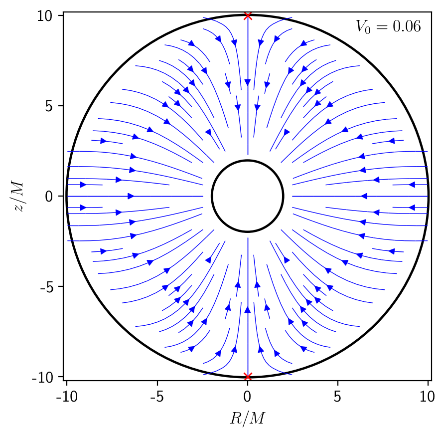
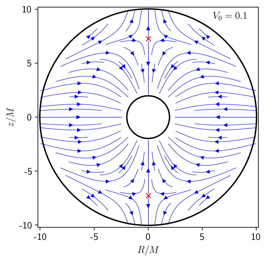
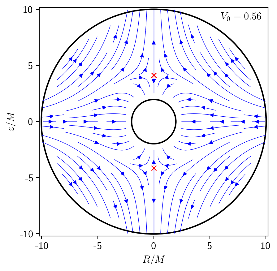
Figure 2: Streamlines of the accretion flow resulting from the velocity field in Eqs. (2.26) and (2.27). We have taken $\mathcal{R}=10M$ as radius of the injection sphere while, from left to right, $V_{0}=0.06,\,0.1,\,0.56$. Note that the first and third values of $V_{0}$ correspond to the lower and upper limits in Eq. (2.35), respectively. The stagnation points in each case are shown as red crosses. The outer boundary of the model $(r=\mathcal{R})$ as well as the event horizon of the central black hole $(r=2M)$ are shown as circles drawn with thick, solid lines. The axes correspond to the usual cylindrical coordinates $R=r\,\sin\theta$, $z=r\,\cos\theta$.

See Figure 2 for three examples of the streamlines resulting from the velocity field in Eqs. (2.26) and (2.27) for $\mathcal{R}=10M$. On the left and right panels $V_{0}=0.06,\,0.56$, which correspond to the lower and upper bounds of the interval in Eq. (2.35). For the central panel we have taken $V_{0}=0.1$ as a representative middle value for $V_{0}$.

In the top panel of Figure 3 we show the magnitude of the three-velocity $V$ as function of the polar angle $\theta$ evaluated at the injection sphere for the particular case $\mathcal{R}=10M$ and several values of $V_{0}$.

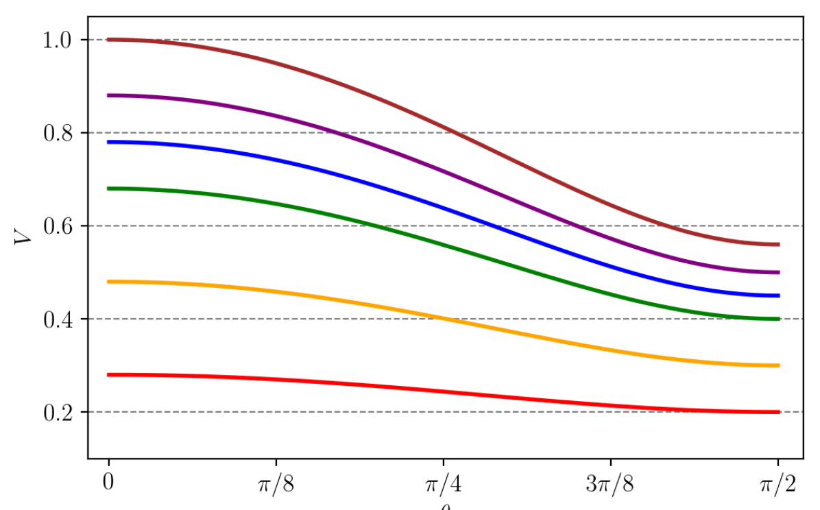
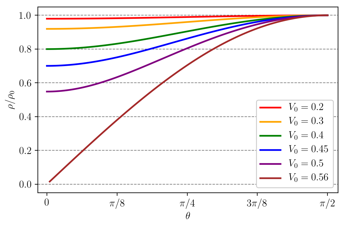
Figure 3: Magnitude of the three-velocity $V$ (Eq. 2.30) and density $\rho$ (Eq. 2.36) of the analytic model for an ultrarelativistic stiff fluid. Both quantities are shown as functions of the polar angle $\theta$ evaluated at the injection sphere for the particular case $\mathcal{R}=10M$ and six different values of the velocity $V_{0}$. In this case, from Eq. (2.32) we have that $V_{0}$ is limited as $V_{0}<0.56$ in order to guarantee that the whole solution is well defined within the spatial domain $r\leq\mathcal{R}$. Note that for $V_{0}=0.56$, $V_{\mathrm{ej}}=1$ while the corresponding value of $\rho$ goes to zero.

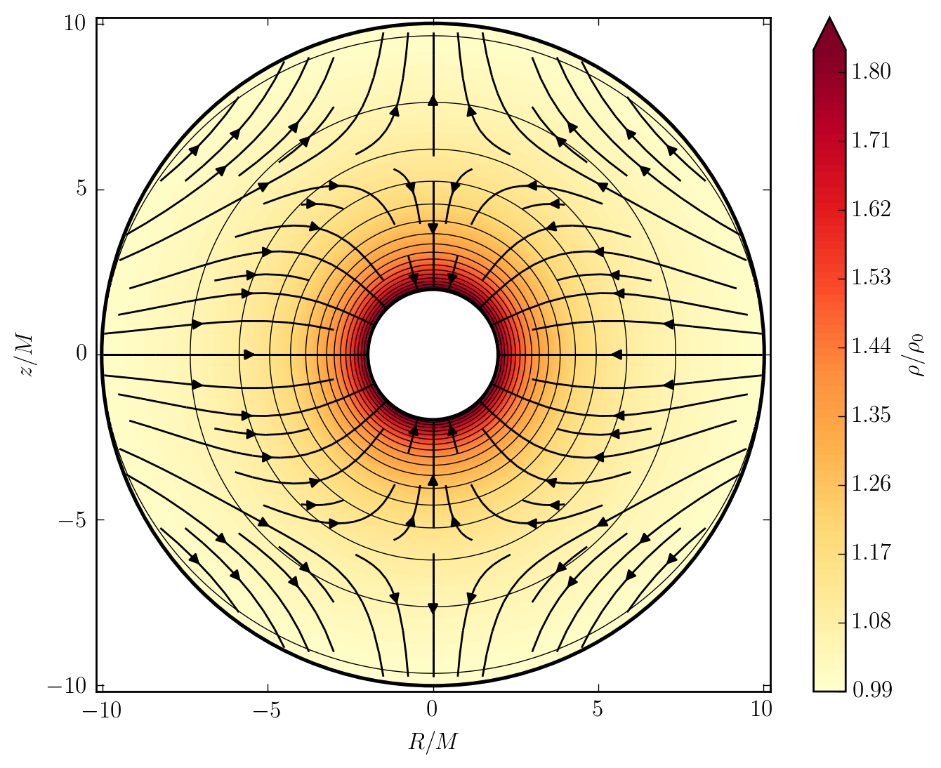
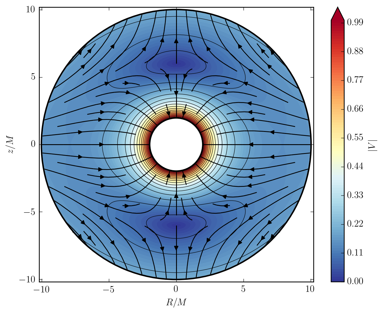
Figure 4: Example of the analytic model of choked accretion for the values $\mathcal{R}=10M$ and $V_{0}=0.16$. The figure shows isocontours of the fluid’s density as given by Eq. (2.36) (left panel) as well as the magnitude of the three-velocity as given by Eq. (2.30) (right panel). Note that the stagnation points are located at $\mathcal{S}=6M$. Fluid streamlines are indicated by thick, solid lines with an arrow. The axes correspond to the usual cylindrical coordinates $R=r\,\sin\theta$, $z=r\,\cos\theta$.

2.3 Density field

We can now recover the density field by substituting Eqs. (2.17)–(2.19) into the normalization condition of the four-velocity $U_{\mu}U^{\mu}=-1$ and then using Eq. (2.20); the result is

$$\frac{\rho}{\rho_{0}}=\frac{\alpha_{0}\,\Gamma_{0}}{\alpha\,\Gamma}=\sqrt{\frac{r(\mathcal{R}-2M)(1-V^{2})}{\mathcal{R}(r-2M)(1-V_{0}^{2})}},$$ (2.36)

with $V^{2}(r,\theta)$ as given in Eq. (2.30).

Recalling that the local density measured by a LEO is given by $D=\Gamma\rho$, from Eq. (2.36) we obtain the interesting result that the density field as described by LEOs is spherically symmetric, i.e. $D$ is only a function of $r$.

Note that the same criterion introduced in Eq. (2.32) in order to guarantee a subluminal three-velocity within $2M<r\leq\mathcal{R}$, also guarantees that the density field as expressed in Eq. (2.36) is a well-defined, real quantity within the same spatial domain.

From Eq. (2.36) we obtain the following simple relation for the ratio between the density at the pole and the equator of the injection sphere

$$\begin{split}\frac{\rho(\mathcal{R},0)}{\rho(\mathcal{R},\pi/2)}&=\frac{\rho(\mathcal{R},0)}{\rho_{0}}=\sqrt{\frac{1-V^{2}_{\mathrm{ej}}}{1-V_{0}^{2}}}\\ &=\sqrt{\frac{\mathcal{R}^{4}-4\,V_{0}^{2}\mathcal{R}^{4}+48V_{0}\mathcal{R}^{2}M^{2}-144M^{4}}{\mathcal{R}^{4}-V_{0}^{2}\mathcal{R}^{4}}}.\end{split}$$ (2.37)

In the following we shall use the contrast $\delta$ between the polar and equatorial densities at the injection sphere defined as

$$\delta=1-\frac{\rho(\mathcal{R},0)}{\rho_{0}}.$$ (2.38)

From Eqs. (2.37) and (2.38) we can see that an arbitrarily small density contrast suffices not only to produce the inflow-outflow configuration shown in the central and right panels of Figure 2, but also to guarantee that $V_{\mathrm{ej}}>V_{0}$. Furthermore notice that, as the density contrast approaches unity, the ejection velocity approaches the speed of light. Indeed, for the present case of an ultrarelativistic stiff fluid, as $\delta\rightarrow 1$ we can obtain arbitrarily large Lorentz factors for the ejected flow.

Complementary to the top panel of Figure 3, where we see that the magnitude of the velocity field at the injection sphere increases as $V_{0}$ increases, in the bottom panel of this figure we show the angular density profile $\rho(\theta)$ evaluated at the injection sphere. From this figure we see that, as $V_{0}$ increases, the polar to equatorial density contrast increases. Moreover, we can also see that as the velocity at the poles becomes luminal for $V_{0}=1/2+6M^{2}/\mathcal{R}^{2}$, the corresponding value of the density field becomes zero.

2.4 Equation for the streamlines

An equation for the streamlines can be found by combining Eqs. (2.26) and (2.27) to obtain

$$\frac{\mathrm{d}r}{\mathrm{d}\theta}=\frac{2-\frac{r(r-M)(r-2M)}{\mathcal{S}(\mathcal{S}-M)(\mathcal{S}-2M)}\left(3\cos^{2}\theta-1\right)}{\frac{3\,r^{2}-6Mr+2M^{2}}{\mathcal{S}(\mathcal{S}-M)(\mathcal{S}-2M)}\sin\theta\cos\theta},$$ (2.39)

which in turn can be integrated as

$$\Psi=\cos\theta\left[1+\frac{r(r-M)(r-2M)}{\mathcal{S}(\mathcal{S}-M)(\mathcal{S}-2M)}\frac{\sin^{2}\theta}{2}\right],$$ (2.40)

where $\Psi$ is an integration constant. Eq. (2.40) constitutes an implicit equation for the streamlines, where, for every constant value of $\Psi$, one has a different streamline. Note in particular that $\Psi=\pm 1$ corresponds to the streamlines reaching the stagnation points located at $(r=\mathcal{S},\,\theta=0)$ for the plus sign and $(r=\mathcal{S},\,\theta=\pi)$ for the minus sign. Streamlines with $|\Psi|<1$ end up accreting onto the central black hole, while those with $|\Psi|>1$ escape along the bipolar outflow.

In Figure 4 we show the resulting density, velocity and streamlines of the analytic model of choked accretion for the particular values of $\mathcal{R}=10M$, $V_{0}=0.16$. For this choice of boundary conditions the stagnation points are located at $\mathcal{S}=6M$.

2.5 Mass accretion, injection and ejection rates

The total mass accretion rate onto the central black hole can be calculated as the flux of mass density integrated over any closed surface $\sigma$ enclosing it, i.e.

$$\dot{M}=-\int_{\sigma}\rho\,U^{\mu}\,\sqrt{-g}\,\mathrm{d}S_{\mu},$$ (2.41)

where $\sqrt{-g}=r^{2}\sin\theta$ and $\mathrm{d}S_{\mu}$ is a differential area element orthogonal to the surface $\sigma$. Taking any sphere of radius $r$ as the integration surface, together with the conditions of axisymmetry and stationarity, we obtain

$$\begin{split}\dot{M}&=-2\pi\int_{0}^{\pi}\rho\,U^{r}\,r^{2}\sin\theta\,\mathrm{d}\theta\\ &=16\pi M^{2}\alpha_{0}\rho_{0}\Gamma_{0}.\end{split}$$ (2.42)

The result of Eq. (2.42) holds even if higher multipoles are considered in the velocity potential (cf. Eq. 2.12): by virtue of the orthogonality of the spherical harmonics, the contribution of any multipole $(l,m)$ to the integral in Eq. (2.42) identically vanishes except for the spherically symmetric monopole $l=0,\,m=0$. Note however that, in the spherically symmetric case, $V_{0}$ is not a free parameter. In accordance with Eq. (2.30), in this case $V_{0}=4M^{2}/\mathcal{R}^{2}$. Therefore, in the spherically symmetric case, the mass accretion rate as given by Eq. (2.42) can be written as

$$\dot{M}_{\mathrm{M}}=16\pi M^{2}\alpha_{0}\rho_{0}\left(1-16\frac{M^{4}}{\mathcal{R}^{4}}\right)^{-1/2}.$$ (2.43)

This value corresponds to the Michel (1972) solution as applied to a stiff equation of state, as shown by Chaverra & Sarbach (2015). See Appendix A for a brief overview of the Michel (1972) model in the case of a general polytrope.

We can express the general result for the mass accretion rate as given in Eq. (2.42) in units of $\dot{M}_{\mathrm{M}}$ as

$$\dot{M}=\eta\,\dot{M}_{\mathrm{M}},$$ (2.44)

where

$$\eta=\left(\frac{1-16M^{4}/\mathcal{R}^{4}}{1-V_{0}^{2}}\right)^{1/2}.$$ (2.45)

Note that in most cases of interest $\eta\gtrsim 1$. For instance, taking $\mathcal{R}=10M$, from the allowed range of velocities in Eq. (2.35), we obtain $1<\eta\lesssim 1.2$, while for $\mathcal{R}\gg M$, we have $1<\eta\lesssim 1.15$.

On the other hand, we can also define the mass injection rate $\dot{M}_{\mathrm{in}}$ as the inward flux of mass across the injection sphere of radius $\mathcal{R}$, i.e. by considering an integration analogous to the one in Eq. (2.42) but in which we consider only the fluid elements with a negative radial velocity $U^{r}$. From Eq. (2.18) we obtain that $U^{r}(\mathcal{R},\theta)<0$ for $\theta_{c}<\theta<\pi-\theta_{c}$, where $\theta_{c}$ is such that $U^{r}(\mathcal{R},\theta_{c})=0$ and is given by

$$\begin{split}\cos\theta_{c}&=\sqrt{\frac{1}{3}+\frac{2}{3}\,\frac{\mathcal{S}(\mathcal{S}-M)(\mathcal{S}-2M)}{\mathcal{R}(\mathcal{R}-M)(\mathcal{R}-2M)}}\\ &=\sqrt{\frac{V_{0}\mathcal{R}^{2}}{3(V_{0}\mathcal{R}^{2}-4M^{2})}}.\end{split}$$ (2.46)

We can thus calculate $\dot{M}_{\mathrm{in}}$ as

$$\dot{M}_{\mathrm{in}}=-4\pi\int_{\theta_{c}}^{\pi/2}\rho\,U^{r}\,r^{2}\sin\theta\,\mathrm{d}\theta=\Lambda\,\dot{M},$$ (2.47)

with

$$\begin{split}\Lambda&=\frac{1}{6\sqrt{3}}\frac{V_{0}\mathcal{R}^{2}}{M^{2}}\left(1-\frac{4M^{2}}{V_{0}\mathcal{R}^{2}}\right)^{-1/2}\\ &\simeq\frac{1}{6\sqrt{3}}\left(\frac{V_{0}\mathcal{R}^{2}}{M^{2}}+2\right)+\mathcal{O}\left(\frac{M^{2}}{V_{0}\mathcal{R}^{2}}\right),\end{split}$$ (2.48)

where for the second step we have used the Taylor series expansion assuming $M^{2}\ll V_{0}\mathcal{R}^{2}$.

From Eq. (2.46) we have that when $V_{0}=6M^{2}/\mathcal{R}^{2}$ (or, equivalently $\mathcal{S}=\mathcal{R}$) then $\theta_{c}=0$ and hence $\dot{M}_{\mathrm{in}}=\dot{M}$. On the other hand, when $V_{0}<6M^{2}/\mathcal{R}^{2}$ we have that $U^{r}<0$ for all $\theta$ and again $\dot{M}_{\mathrm{in}}=\dot{M}$. We can then write

$$\dot{M}_{\mathrm{in}}=\begin{cases}\dot{M},&\text{if}\ V_{0}\leq 6M^{2}/\mathcal{R}^{2},\\ \Lambda\,\dot{M},&\text{if}\ V_{0}>6M^{2}/\mathcal{R}^{2}.\end{cases}$$ (2.49)

Similarly, we define the mass ejection rate $\dot{M}_{\mathrm{ej}}$ as the outward flux of mass across the sphere of radius $r=\mathcal{R}$. Clearly

$$\dot{M}_{\mathrm{ej}}=\begin{cases}0,&\text{if}\ V_{0}\leq 6M^{2}/\mathcal{R}^{2},\\ (\Lambda-1)\dot{M},&\text{if}\ V_{0}>6M^{2}/\mathcal{R}^{2}.\end{cases}$$ (2.50)

Note that for a fixed injection radius $\mathcal{R}$, it can be shown that the upper bound for $V_{0}$ found in Eq. (2.32) implies the following upper bound for the mass injection rate

$$\dot{M}_{\mathrm{in}}<8\pi\,\rho_{0}\sqrt{\frac{(\mathcal{R}-2M)\mathcal{R}^{3}(\mathcal{R}^{2}+12M^{2})^{3}}{3(\mathcal{R}^{2}+4M^{2})[4\mathcal{R}^{4}-(\mathcal{R}^{2}+12M^{2})^{2}]}}.$$ (2.51)

The Eqs. (2.49) and (2.50) encapsulate the concept of choked accretion described in the introduction: the central black hole accretes at an essentially fixed rate $\dot{M}\simeq\dot{M}_{\mathrm{M}}$. Whenever the mass injection rate surpasses this limit, the excess flux is ejected from the system as a bipolar outflow at the rate $\dot{M}_{\mathrm{ej}}$. Note in particular that from Eq. (2.50) we can write

$$\frac{\dot{M}_{\mathrm{ej}}}{\dot{M}_{\mathrm{in}}}=1-\frac{\dot{M}}{\dot{M}_{\mathrm{in}}}=1-\frac{1}{\Lambda}.$$ (2.52)

This simple functional dependence of the ratio of ejected to injected mass fluxes on the injection mass rate is shown in Figure 14 to compare the analytic model against the results of hydrodynamic numerical simulations.

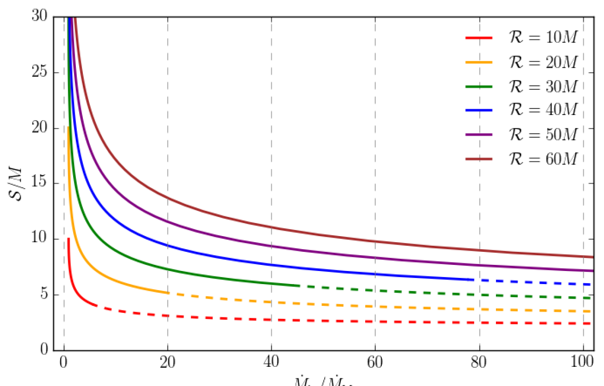
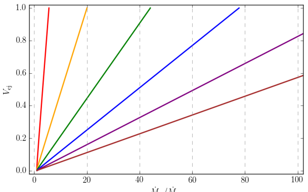
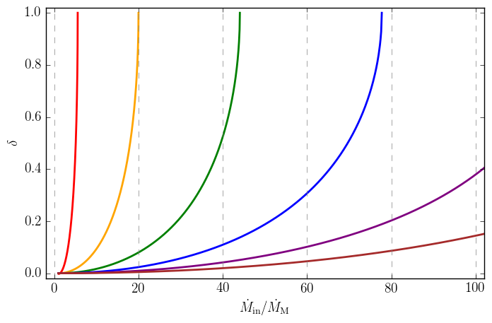
Figure 5: Dependence of different properties of the analytic model of choked accretion on the parameters $\mathcal{R}/M$ and $\dot{M}_{\mathrm{in}}/\dot{M}_{\mathrm{M}}$. From top to bottom, each panel shows: the location of the stagnation point $\mathcal{S}$, the maximum velocity attained by the ejected material $V_{\mathrm{ej}}$ (Eq. 2.31), and the density contrast between the pole and the equator of the injection sphere $\delta$ (Eq. 2.38). The dashed lines in the top panel indicate regions in the parameter space for which the model is not well defined within the whole domain $r<\mathcal{R}$ (see discussion in the main text).

Finally, it is interesting to explore the behavior of the analytic model as a function of the parameters $\mathcal{R}$ and $\dot{M}_{\mathrm{in}}/\dot{M}_{\mathrm{M}}=\eta\,\Lambda$. Note that, as shown in Eq. (2.48), $\eta\,\Lambda$ is essentially a linear reparametrization of $V_{0}$ for most of the domain of interest. In Figure 5 we show the dependence on these parameters of the location of the stagnation point $\mathcal{S}$ (cf. Eq. 2.23), the maximum velocity attained by the ejected material $V_{\mathrm{ej}}$ (cf. Eq. 2.33), and the contrast $\delta$ between the polar and equatorial densities at the injection sphere (cf. Eq. 2.38).

From this figure we see that as $\dot{M}_{\mathrm{in}}/\dot{M}_{\mathrm{M}}$ increases the stagnation point sinks closer to the central accretor, while at the same time the velocity of the ejected material approaches the speed of light and the density contrast increases. From Eq. (2.52) and Figure 14 it is also clear that as the injection rate increases, more and more material is expelled from the system as a bipolar outflow. Moreover, the restrictions on the model parameters, as established in Eqs. (2.32) and (2.51), are also apparent in Figure 5: as soon as these limits are exceeded, the model ceases to be well-defined within the whole domain $r<\mathcal{R}$.

The non-relativistic limit of an ultrarelativistic, stiff fluid corresponds to an incompressible fluid (Tejeda, 2018). This Newtonian counterpart of the present analytic model is discussed in Aguayo-Ortiz et al. (2019). Indeed, it is simple to verify that, in the limit in which $V_{0}\ll 1$ and $\mathcal{R}\gg M$, all of the equations derived in this section for the velocity field, the streamlines, and the different mass fluxes reduce to the expressions presented in Aguayo-Ortiz et al. (2019).

The analytic model that we have presented allows a transparent understanding of the physics involved in the choked accretion mechanism. However, generalizing this model to accommodate a more realistic equation of state becomes analytically intractable. We explore this generalization in the next section by means of numerical simulations.

3 Numerical simulations

The main limitation of the analytic model for choked accretion discussed in the previous section is that it is based on the assumption of an ultrarelativistic gas with a stiff equation of state, an assumption with a rather restricted applicability in astrophysics. In this section we want to explore whether the phenomenon of choked accretion might also arise when considering more general equations of state, thus relaxing the associated assumption of a potential flow. This exploration will be based on full-hydrodynamic, numerical simulations performed with the open source code aztekas.

The general relativistic hydrodynamic equations are solved numerically with aztekas by recasting them in a conservative form using the Valencia formulation (Banyuls et al., 1997). The aztekas code uses a grid based finite volume scheme, a High Resolution Shock Capturing method with an approximate Riemann solver for the flux calculation, and a monotonically centered second order reconstructor at cell interfaces. The code adopts a second order total variation diminishing Runge-Kutta method (Shu & Osher, 1988) for the time integration. See Tejeda & Aguayo-Ortiz (2019) for further details about the discretization used in aztekas. Code validation through comparisons to standard analytical solutions in the Newtonian and relativistic regimes can be found in Aguayo-Ortiz et al. (2018); Tejeda & Aguayo-Ortiz (2019); Aguayo-Ortiz et al. (2019), while a number of standard shock tube tests successfully reproduced by the code are included in Appendix B.

The simulations presented in this section were performed for a perfect fluid evolving in a fixed, background metric corresponding to a Schwarzschild black hole of mass $M$. We adopt horizon-penetrating, Kerr-Schild coordinates and, imposing axisymmetry, we consider only 2D spatial domains with spherical coordinates $r$ and $\theta$.

Furthermore, by assuming symmetry with respect to the equatorial plane located at $\theta=\pi/2$ (north-south symmetry), we restrict the numerical domain as $(r,\,\theta)\in[\mathcal{R}_{\text{acc}},\,\mathcal{R}]\times[0,\,\pi/2]$, where $\mathcal{R}_{\text{acc}}$ is the radius of the inner boundary at which we adopt a free outflow condition (i.e. free inflow onto the central black hole) and $\mathcal{R}$ is the radius of the injection sphere at which we impose a given profile for the physical parameters of the injected fluid. At both polar boundaries $\theta=0,\,\pi/2$ we adopt reflection conditions.

As initial conditions, we populate the whole numerical domain with the same values as those used at the outer boundary $\mathcal{R}$. For the code we adopt geometrized units, and take $M=1$ as unit of length and time.

3.1 Stiff fluid

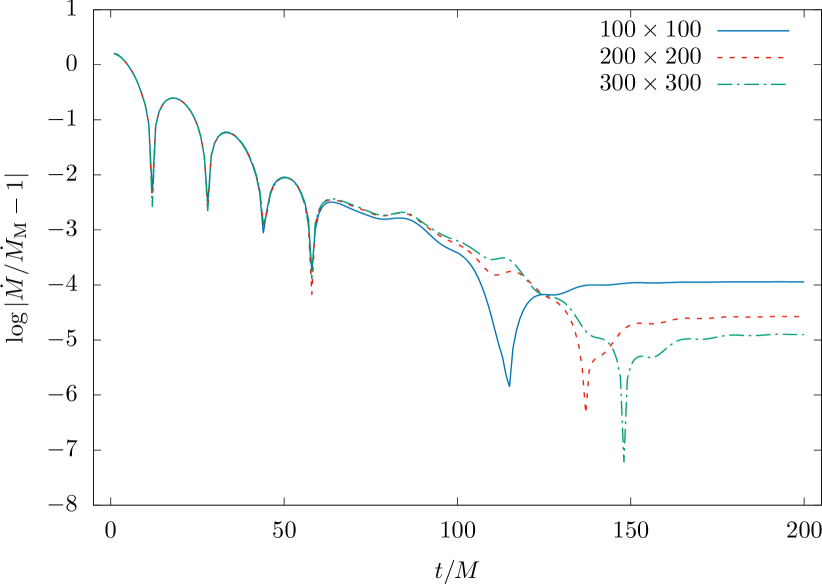
Figure 6: Benchmark test of aztekas with the analytic model of choked accretion described in Section 2. In this case we took $\mathcal{R}=10M$ as radius of the injection sphere and $V_{0}=0.16$ at the equator. The figure shows the time evolution of the relative error between the numerically calculated accretion rate $\dot{M}$ and the exact value of $\dot{M}_{\mathrm{M}}=16\pi M^{2}\alpha_{0}\rho_{0}\Gamma_{0}$ for three resolutions (grid points) 100$\times$100, 200$\times$200, and 300$\times$300. Note that the sharp falls observed in this figure correspond to changes in sign of the relative error being plotted. Moreover, the apparent periodicity observed at the beginning of the curve corresponds to an initial transient mode reflecting back and forth throughout the numerical domain at the speed of sound (in this case, the sound crossing time is $t\sim 10M$).

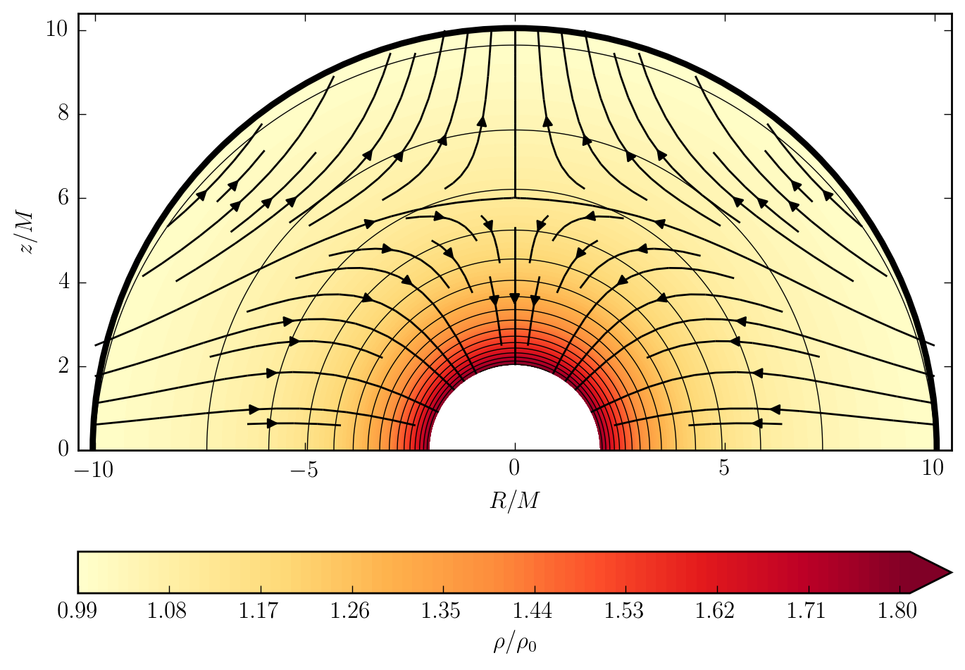
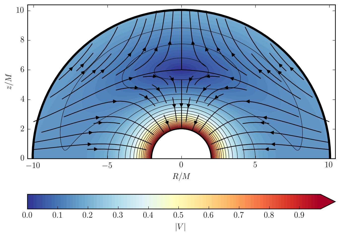
Figure 7: Benchmark test of aztekas with the analytic model of choked accretion described in Section 2. In this case we took $\mathcal{R}=10M$ as radius of the injection sphere and $V_{0}=0.16$ at the equator. The left panel shows isocontour levels of the density field with the scale indicated by the color bar. The right panel shows isocontour levels of the magnitude of the three-velocity. Fluid streamlines are indicated by thick, solid lines with an arrow. The simulation time is $t=650M$. An excellent agreement is found between this figure and its analytic counterpart in Figure 4.

An analytic model can be useful as a benchmark solution for testing the ability of a numerical code to recover certain behaviour under appropriate conditions. Here we use the exact analytic solution presented in the previous section as a benchmark test for aztekas. Specifically, we will consider the values of $\mathcal{R}=10M$ for the radius of the injection sphere and $V_{0}=0.16$ for the magnitude of the three-velocity at the equator of the injection sphere.

For this test we take as radial boundaries $\mathcal{R}_{\text{acc}}=M$ and $\mathcal{R}=10M$ and use three different resolutions (grid points) 100$\times$100, 200$\times$200, and 300$\times$300 for the radial and polar ranges. We adopt the approximation of an ultrarelativistic gas with a stiff equation of state as described in Section 2. At the injection sphere we impose the analytic value for the density as given in Eq. (2.36) and the velocity components corresponding to the transformation from Schwarzschild coordinates to Kerr-Schild coordinates.

We let the simulations run until a steady-state condition is reached. This is monitored by calculating the mass accretion rate $\dot{M}$ across $\mathcal{R}_{\text{acc}}$. In Figure 6 we show the time evolution of the numerically calculated $\dot{M}$ as compared to the analytically expected value of $\dot{M}_{\mathrm{M}}=16\pi M^{2}\alpha_{0}\rho_{0}\Gamma_{0}$ for the three adopted resolutions. As can be seen from this figure, the value of $\dot{M}$ rapidly stabilizes to a constant value that agrees with $\dot{M}_{\mathrm{M}}$ to within $0.001\%$ for the largest resolution considered.

In Figure 7 we show the density and velocity fields of the aztekas simulation at $t=650M$. The stagnation point in the numerical simulation is located at $\mathcal{S}=6.0175M$, which is consistent with the analytically exact value of $\mathcal{S}=6M$, taking into account the radial grid size of $\Delta r=0.045M$.

We have also tried this benchmark test with different values of $\mathcal{R}$ and $V_{0}$, and consistently found that the numerical results recover the analytic solution in this limit case of a stiff equation of state, thus validating our numerical setup.

3.2 Polytropic fluids

In this section we relax the stiff fluid condition and consider perfect fluids described by a polytropic equation of state of the form

$$P=K\,\rho^{\gamma},$$ (3.1)

with $\rho$ the rest mass density, $\gamma$ the adiabatic index, and $K=\mathrm{const.}$ From Eq. (2.3), the sound speed corresponding to this equation of state is given by

$$a^{2}=\frac{\gamma}{h}\frac{P}{\rho},$$ (3.2)

where $h$ is the relativistic specific enthalpy. For a perfect fluid described by Eq. (3.1), $h$ is related to the other thermodynamical variables through

$$h=1+\frac{\gamma}{\gamma-1}\frac{P}{\rho},$$ (3.3)

or, by combining Eqs. (3.2) and (3.3), we can also write

$$h=\frac{1}{1-a^{2}/(\gamma-1)}.$$ (3.4)

The expected requirement for the appearance of choked accretion, is that there should exist a small contrast between the density at the equator and that at the poles of the injection sphere. Here we impose this density contrast by adopting the following density profile as boundary condition at the injection radius $\mathcal{R}$

$$\rho(\theta)=\rho_{0}\left(1-\delta\cos^{2}\theta\right),$$ (3.5)

where $\rho_{0}$ is the value of the density at the equator of the injection sphere, i.e $\rho_{0}=\rho(\pi/2)$, and $\delta$ is the same density contrast between the equator and the poles as defined in Eq. (2.38).

The specific functional form of the boundary condition in Eq. (3.5) was chosen as a convenient first-order parametrization of a bipolar deviation from spherical symmetry. This profile is qualitatively similar to the one of the analytic model presented above (see bottom panel of Figure 4). We have explored with other similar boundary profiles and obtained consistent results.

For the simulations reported in this work we have taken $\rho_{0}=10^{-10}$, although we have found that taking any other value of $\rho_{0}$ results in the same flow structure but with the density re-scaled by this new factor. In other words, the value of $\rho_{0}$ can be set arbitrarily, thus defining a unit scale for the density and related thermodynamical quantities, provided the fluid considered remains a negligible perturbation on the background metric. On the other hand, the resulting steady state solution depends strongly on the value of the sound speed $a_{0}$ imposed at the equator of the injection sphere. Note in particular that, from Eq. (3.4) and for a fixed adiabatic index $\gamma$, $a_{0}$ is limited as

$$0<a_{0}<\sqrt{\gamma-1}.$$ (3.6)

Once we have adopted a given $\gamma$, set up values for $\rho_{0}$ and $a_{0}$ at the equator of the injection sphere and a density contrast $\delta$, we use the equation of state in Eq. (3.1) to find the corresponding pressure profile at the injection boundary as

$$P(\theta)=\frac{1}{\gamma}\left[\frac{a^{2}_{0}}{1-a^{2}_{0}/(\gamma-1)}\right]\frac{\rho(\theta)^{\gamma}}{\rho_{0}^{\gamma-1}}.$$ (3.7)

Since we do not know the structure of the accretion flow beforehand (on which no a priori restrictions are imposed), we can not prescribe specific values for the velocity components at the injection radius. For this reason we adopt free-boundary conditions for the radial and polar components of the velocity field and let the simulation evolve starting off from an initial state at rest (zero initial velocities), until an equilibrium state is reached throughout the numerical domain. Note that this means that we can not use the same parametrization that we had adopted for the analytic model of Section 2 (i.e. $\mathcal{R}/M$, $\rho_{0}$, $P_{0}$, and $V_{0}$), but instead now we shall replace $V_{0}$ by the density contrast $\delta$.

3.2.1 Dependence on the density contrast $\delta$

Based on the analytic results of Section 2, we expect ejection rates and velocities to strongly correlate with the density contrast at the injection surface. Here we study the role of the density contrast as parametrized by $\delta$ in Eq. (3.5). In Figure 8 we show the steady-state results for four numerical simulations with $\gamma=4/3$, $a_{0}=0.5$, $\mathcal{R}=10M$, and density contrasts $\delta=0,\,0.1,\,0.3$ and 0.9. The results of these four simulations, including also the $\delta=0.5$ case, are reported in Table 1. We can see that, as soon as the equatorial region becomes over dense with respect to the polar regions, i.e. $\delta>0$, a strong qualitative change ensues with an inflow-outflow configuration appearing across the numerical domain. The resulting streamlines closely resemble the flow morphology of the analytic model presented in the previous section.

We can also see that as the density contrast increases, both $\dot{M}$ and $\dot{M}_{\mathrm{in}}$ increase. Note however, that $\dot{M}_{\mathrm{in}}$ increases faster than $\dot{M}$, with the net result that the ratio between ejection and injection also increases with increasing $\delta$.

As a further positive test of our numerical scheme, when $\delta=0$ the simulation recovers the analytic solution of spherically symmetric accretion discussed by Michel (1972). The sixth column in Table 1 reports the ratio $\dot{M}/\dot{M}_{\mathrm{M}}$, i.e. the numerically found mass accretion rate in units of the mass accretion rate of Michel’s solution $\dot{M}_{\mathrm{M}}$ (an analytic expression for $\dot{M}_{\mathrm{M}}$ is derived in Appendix A). Note that, as occurs also in the analytic model discussed in the previous section, this ratio does not remain strictly equal to one as $\delta$ increases, although the mass accretion rate remains of the order of $\dot{M}_{\mathrm{M}}$.

This first exploration confirms that the basic principle behind the choked accretion model presented in Section 2 also works for fluids described by more general equations of state, where the resulting flow pattern is no longer assumed to be a potential flow.

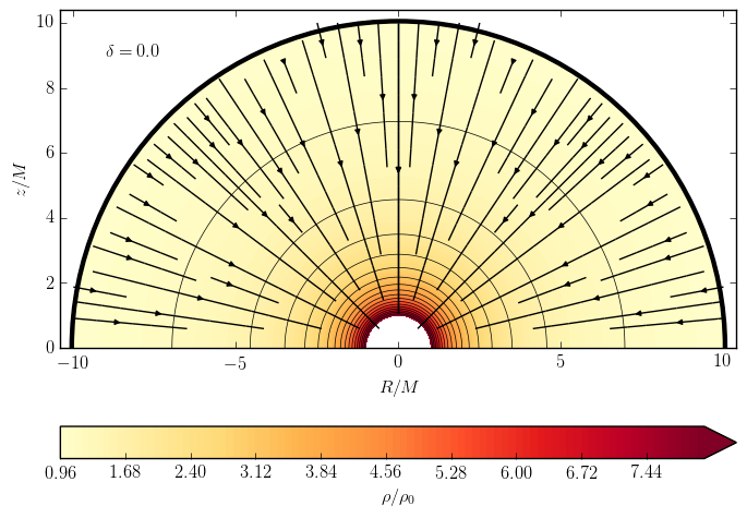
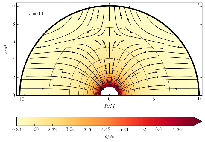
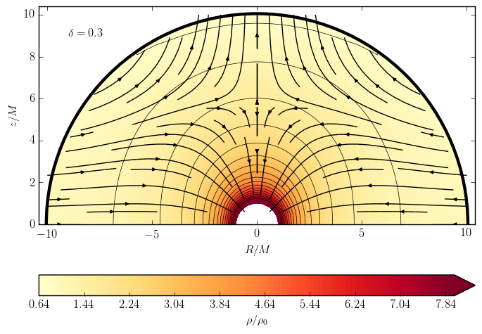
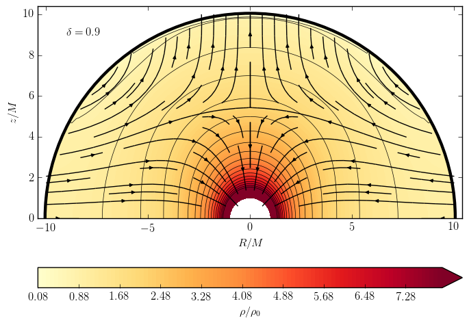
Figure 8: Resulting steady state flow configuration for the numerical simulations for a polytropic fluid with $\gamma=4/3$ accreting onto a Schwarzschild black hole. The value of the density contrast $\delta$ used in each case is indicated on the top-left corner of each panel, and increases gradually from $\delta=0$ in the first panel (isotropic case where the Michel solution is recovered) to the highly anisotropic $\delta=0.9$ case in the fourth panel.

Table 1: Dependence on the density contrast $\delta$

$\delta$	$\dot{M}$	$\dot{M}_{\mathrm{in}}$	$\dot{M}_{\mathrm{ej}}$	$\frac{\dot{M}_{\mathrm{ej}}}{\dot{M}_{\mathrm{in}}}$	$\frac{\dot{M}}{\dot{M}_{\mathrm{M}}}$	$\mathcal{S}$	$V_{\mathrm{ej}}$
0.0	9.08	9.08	0.0	0.0	1.0	…	…
0.1	9.55	11.16	1.61	0.14	1.05	6.63	0.25
0.3	10.35	14.10	3.75	0.27	1.14	5.91	0.43
0.5	11.14	16.24	5.10	0.31	1.23	5.64	0.46
0.9	12.81	19.77	6.96	0.35	1.41	5.46	0.47

Note. — The simulation parameters are fixed as $\mathcal{R}=10M$, $\gamma=4/3$ and $a_{0}=0.5$. All the accretion rates are expressed in units of $\dot{M}_{0}=M^{2}\rho_{0}$, and the stagnation point in units of $M$. The velocity $V_{\mathrm{ej}}$ is defined as the magnitude of the three-velocity at the poles of the injection sphere. According to Eq. (A.15), the Michel mass accretion rate in this case is given by $\dot{M}_{\mathrm{M}}=9.08\dot{M}_{0}$.

3.2.2 Dependence on the adiabatic index $\gamma$

Here we examine the behaviour of the steady-state, numerical solution as a function of the adiabatic index $\gamma$. We keep as fixed parameters $\mathcal{R}=10M$, $\delta=0.3$ and $a_{0}=0.5$ while considering four different values of $\gamma=4/3,\,3/2,\,5/3$, and 2. In Table 2 we summarize the results of these simulations, while in Figure 9 we plot the ratios $\dot{M}/\dot{M}_{\mathrm{M}}$, $\dot{M}_{\mathrm{in}}/\dot{M}_{\mathrm{M}}$ and $\dot{M}_{\mathrm{ej}}/\dot{M}_{\mathrm{M}}$ as functions of $\gamma$. The resulting density field and fluid streamlines for these four simulations are qualitatively similar to those shown in the bottom left panel of Figure 8.

Table 2: Dependence on the adiabatic index $\gamma$

$\gamma$	$\dot{M}$	$\dot{M}_{\mathrm{in}}$	$\dot{M}_{\mathrm{ej}}$	$\frac{\dot{M}_{\mathrm{ej}}}{\dot{M}_{\mathrm{in}}}$	$\frac{\dot{M}}{\dot{M}_{\mathrm{M}}}$	$\mathcal{S}$	$V_{\mathrm{ej}}$
4/3	10.35	14.10	3.75	0.27	1.14	5.91	0.43
3/2	9.75	13.61	3.86	0.28	1.12	5.82	0.42
5/3	9.15	13.12	3.96	0.30	1.10	5.73	0.41
2	8.01	12.16	4.15	0.34	1.07	5.55	0.40

Note. — The simulation parameters are $\mathcal{R}=10M$, $a_{0}=0.5$ and $\delta=0.3$. From top to bottom the values of $\dot{M}_{\mathrm{M}}/\dot{M}_{0}$ are 9.08, 8.70, 8.28 and 7.47.

Table 3: Dependence on the density contrast $\delta$ for $a_{0}=0.2$

$\delta[\%]$	$\dot{M}$	$\dot{M}_{\mathrm{in}}$	$\dot{M}_{\mathrm{ej}}$	$\frac{\dot{M}_{\mathrm{ej}}}{\dot{M}_{\mathrm{in}}}$	$\frac{\dot{M}}{\dot{M}_{\mathrm{M}}}$	$\mathcal{S}$	$V_{\mathrm{ej}}$
0.1	63.12	70.50	7.37	0.10	0.98	66.28	0.014
0.5	63.93	89.90	25.97	0.29	0.99	56.78	0.025
1.0	64.13	97.61	33.49	0.34	1.00	51.08	0.031
5.0	64.78	159.93	95.15	0.59	1.01	39.68	0.071

Note. — The sound speed $a_{0}$ is given at the equator of the injection sphere. The simulation parameters are $\mathcal{R}=100M$ and $\gamma=5/3$. In this case $\dot{M}_{\mathrm{M}}=64.39\dot{M}_{0}$.

Table 4: Dependence on the density contrast $\delta$ for $a_{0}=0.4$

$\delta[\%]$	$\dot{M}$	$\dot{M}_{\mathrm{in}}$	$\dot{M}_{\mathrm{ej}}$	$\frac{\dot{M}_{\mathrm{ej}}}{\dot{M}_{\mathrm{in}}}$	$\frac{\dot{M}}{\dot{M}_{\mathrm{M}}}$	$\mathcal{S}$	$V_{\mathrm{ej}}$
0.1	17.49	43.25	25.76	0.60	1.10	42.53	0.019
0.5	17.14	79.47	62.33	0.78	1.08	33.03	0.043
1.0	16.49	106.08	89.60	0.84	1.04	29.23	0.061
5.0	17.74	222.67	204.93	0.92	1.11	22.58	0.136

Note. — The sound speed $a_{0}$ is given at the equator of the injection sphere. The simulation parameters are $\mathcal{R}=100M$ and $\gamma=5/3$. In this case $\dot{M}_{\mathrm{M}}=15.93\dot{M}_{0}$.

Table 5: Dependence on the density contrast $\delta$ for $a_{0}=0.6$

$\delta[\%]$	$\dot{M}$	$\dot{M}_{\mathrm{in}}$	$\dot{M}_{\mathrm{ej}}$	$\frac{\dot{M}_{\mathrm{ej}}}{\dot{M}_{\mathrm{in}}}$	$\frac{\dot{M}}{\dot{M}_{\mathrm{M}}}$	$\mathcal{S}$	$V_{\mathrm{ej}}$
0.1	10.82	52.63	41.81	0.79	1.32	33.03	0.029
0.5	11.35	108.20	96.85	0.90	1.39	25.43	0.064
1.0	10.37	147.74	137.37	0.93	1.27	22.58	0.091
5.0	10.76	318.85	308.09	0.97	1.32	17.83	0.202

Note. — The sound speed $a_{0}$ is given at the equator of the injection sphere. The simulation parameters are $\mathcal{R}=100M$ and $\gamma=5/3$. In this case $\dot{M}_{\mathrm{M}}=8.17\dot{M}_{0}$.

Table 6: Dependence on the density contrast $\delta$ for $a_{0}=0.8$

$\delta[\%]$	$\dot{M}$	$\dot{M}_{\mathrm{in}}$	$\dot{M}_{\mathrm{ej}}$	$\frac{\dot{M}_{\mathrm{ej}}}{\dot{M}_{\mathrm{in}}}$	$\frac{\dot{M}}{\dot{M}_{\mathrm{M}}}$	$\mathcal{S}$	$V_{\mathrm{ej}}$
0.1	7.77	64.80	57.04	0.88	1.41	28.28	0.038
0.5	9.20	139.98	130.78	0.93	1.67	21.63	0.085
1.0	9.20	194.61	185.40	0.95	1.67	19.73	0.120
5.0	8.14	422.31	414.17	0.98	1.48	14.98	0.268

Note. — The sound speed $a_{0}$ is given at the equator of the injection sphere. The simulation parameters are $\mathcal{R}=100M$ and $\gamma=5/3$. In this case $\dot{M}_{\mathrm{M}}=5.50\dot{M}_{0}$.

From these results we see a weak dependence on the adiabatic index $\gamma$. As we consider increasing values of $\gamma$, the values of $\dot{M}$, $\dot{M}_{\mathrm{in}}$, $\mathcal{S}$ and $V_{\mathrm{ej}}$ slightly decrease while both $\dot{M}_{\mathrm{ej}}$ and the ratio $\dot{M}_{\mathrm{ej}}/\dot{M}_{\mathrm{in}}$ increase.

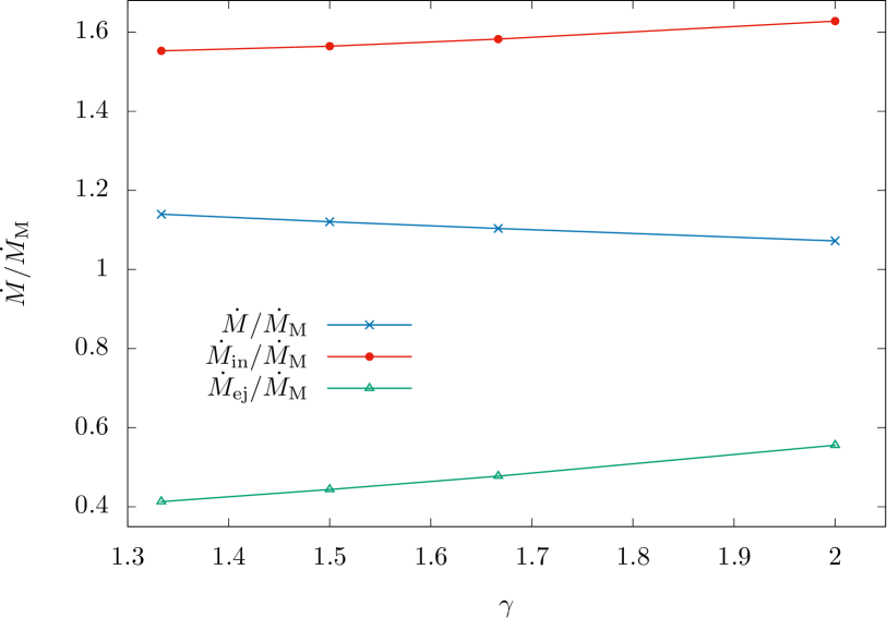
Figure 9: Dependence of the different mass flux rates (in units of the corresponding Michel value $\dot{M}_{\mathrm{M}}$) on the polytropic index $\gamma$.

3.2.3 Dependence on the sound speed $a_{0}$

Now we turn our attention to the role played by the sound speed as defined at the equator of the injection sphere, $a_{0}$. We will also consider a larger injection radius than in the previous sections in order to probe a different regime with smaller density contrasts and larger mass injection rates. Specifically, we take $\mathcal{R}=100M$, $\gamma=5/3$, four density contrasts: $\delta=$ 0.1, 0.5, 1.0, 5.0 %, and four different values for the sound speed: $a_{0}=0.2$, 0.4, 0.6, and 0.8. Note that, from Eq. (3.6) for $\gamma=5/3$, the maximum possible value for this parameter is $a_{0}=0.816$.

In Tables 3–6, we present a summary of the results obtained in this case. In Figure 10 we show the dependence of the ratio $\dot{M}_{\mathrm{in}}/\dot{M}_{\mathrm{M}}$ on $a_{0}$ for the four values of the density contrast $\delta$. Figure 11 shows the dependence of the location of the stagnation point $\mathcal{S}$ on $a_{0}$, while Figure 12 shows the dependence of the maximum velocity of the ejected material $V_{\mathrm{ej}}$ on $a_{0}$.

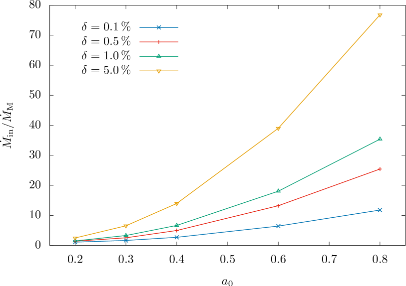
Figure 10: Dependence of the ratio $\dot{M}_{\mathrm{in}}/\dot{M}_{\mathrm{M}}$ on the sound speed $a_{0}$ as given at the equator of the injection sphere. Clearly this ratio is a monotonically increasing function of $a_{0}$ with a steeper growth with increasing $\delta$.

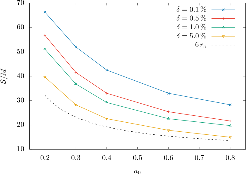
Figure 11: Dependence of the location of the stagnation point $\mathcal{S}$ on $a_{0}$. Here we see that $\mathcal{S}$ is inversely proportional to both $a_{0}$ and $\delta$. Note that $\mathcal{S}$ shows a dependence on $a_{0}$ that resembles the one followed by the critical radius $r_{c}$ on this same parameter.

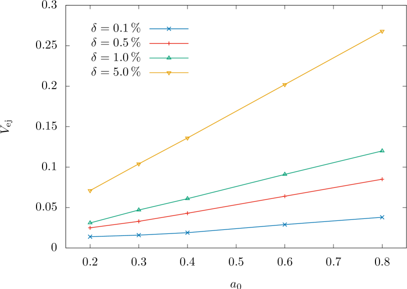
Figure 12: Dependence of the maximum velocity of the ejected material $V_{\mathrm{ej}}$ on $a_{0}$. Here we see that $V_{\mathrm{ej}}$ grows more or less linearly with $a_{0}$.

It is interesting to notice from Figure 11 that, at least for the parameter space explored for this figure, $\mathcal{S}$ follows a dependence on $a_{0}$ similar to the one followed by the critical radius $r_{c}$ as defined in Appendix A for the accretion flow in the spherically symmetric case.

In Figure 13 we show the resulting steady flow configurations for the four values of $a_{0}$ in Tables 3–6 and $\delta=0.5\,\%$. The corresponding configurations for the other values of $\delta$ are qualitatively similar to the ones presented in this figure.

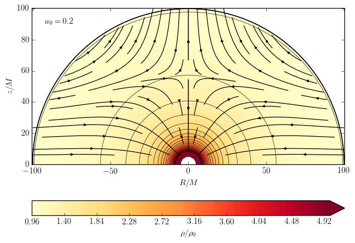
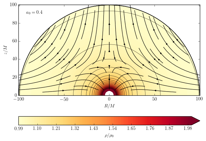
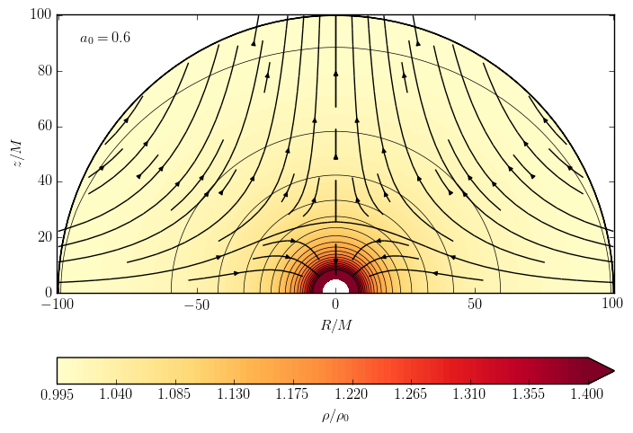
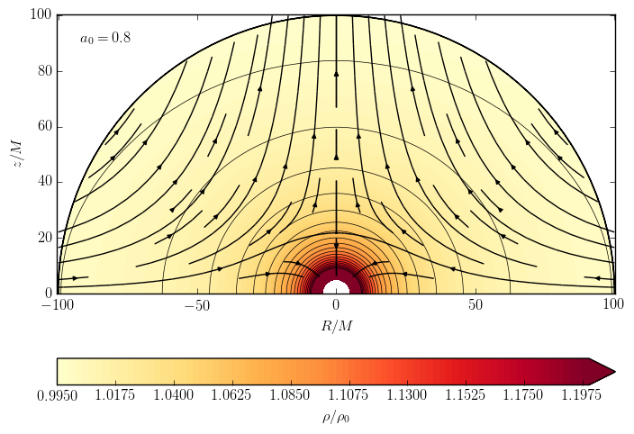
Figure 13: Resulting steady state configurations for a polytropic fluid with $\gamma=5/3$ and $\delta=0.5\,\%$. The value of the sound speed $a_{0}$ used in each case is indicated on the top-left corner of each panel.

From these results we see that the final steady state configuration depends strongly on the value of the sound speed $a_{0}$. In general we see that as $a_{0}$ increases, the stagnation point $\mathcal{S}$ sinks deeper into the accretion flow, as more material is expelled from the system along the bipolar outflow at increasingly larger speeds $V_{\mathrm{ej}}$. Moreover, we also see that as the influx asymmetry increases, even for a small $5\%$ density contrast, the ejection velocities become larger, reaching values of $V_{\mathrm{ej}}>0.25$ for the sound speed values probed.

4 Discussion

4.1 Comparison between the numerical simulations and the analytic model

Even though the physics of the analytic model of Section 2 differs from the one included in the simulations of Section 3, it is illustrative to compare the results of these two sections. For this comparison we will consider only the case of the $\gamma=5/3$ polytrope and injection radius $\mathcal{R}=100M$ presented in Tables 3–6, as this large injection radius allowed us to explore a broader range of mass injection rates.

In Figure 14 we show the ratio of ejected over injected mass rates $\dot{M}_{\mathrm{ej}}/\dot{M}_{\mathrm{in}}$ as a function of the mass injection rate. From this figure we find a very good agreement between the numerical data and the analytic model. This agreement is remarkable if we take into account that the latter is based on the assumption of an ultrarelativistic stiff fluid, $\gamma=2$, while the former involves a more realistic $\gamma=5/3$ polytrope. We have also found this same agreement for different polytropic indices in the non-relativistic regime, as can be seen in Figure 7 of Aguayo-Ortiz et al. (2019).

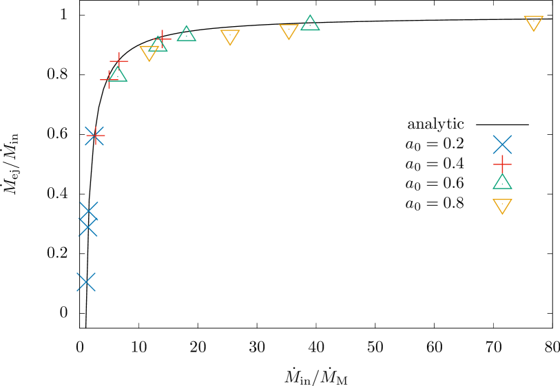
Figure 14: Ratio of ejected to injected mass rates $\dot{M}_{\mathrm{ej}}/\dot{M}_{\mathrm{in}}$ as a function of the injection mass rate in units of the Michel value $\dot{M}_{\mathrm{M}}$. The injection radius is $\mathcal{R}=100M$. The different symbols correspond to the numerical results reported in Tables 3–6 for $\gamma=5/3$ and sound speeds as labeled. The solid line corresponds to the analytic model of an ultrarelativistic $\gamma=2$ stiff fluid presented in Section 2 (cf. Eq. 2.52).

In Figure 15 we show the location of the stagnation point $\mathcal{S}$ as a function of the injection mass rate $\dot{M}_{\mathrm{in}}/\dot{M}_{\mathrm{M}}$. Note that as $\dot{M}_{\mathrm{in}}$ increases, $\mathcal{S}$ descends towards the central accretor, just as it occurred for the analytic model (cf. Figure 5). We find again a good agreement between the numerical data and the analytic model.

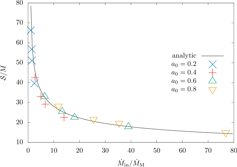
Figure 15: Location of the stagnation point $\mathcal{S}$ as a function of the injection mass rate. The injection radius is $\mathcal{R}=100M$. The different symbols correspond to the numerical results reported in Tables 3–6 for $\gamma=5/3$ and sound speeds as labeled. The solid line corresponds to the analytic model of an ultrarelativistic $\gamma=2$ stiff fluid presented in Section 2.

In Figure 16 we show the maximum velocity attained by the ejected material $V_{\mathrm{ej}}$ as a function of the injection mass rate $\dot{M}_{\mathrm{in}}/\dot{M}_{\mathrm{M}}$. We compare the numerical results against the analytic value for $V_{\mathrm{ej}}$ given in Eq. (2.31). In contrast to what happens for the two parameters discussed above, here we find a large difference among the numerical results for each value of the sound speed $a_{0}$, as well as between these results and the analytic model. Note, however, that for each value of $a_{0}$ the numerically obtained values of $V_{\mathrm{ej}}$ follow a linear dependence on $\dot{M}_{\mathrm{in}}/\dot{M}_{\mathrm{M}}$ with a slope inversely proportional to $a_{0}$. Also, as $a_{0}$ increases the numerical data approaches the analytic model, for which $a=1$ everywhere in the fluid.

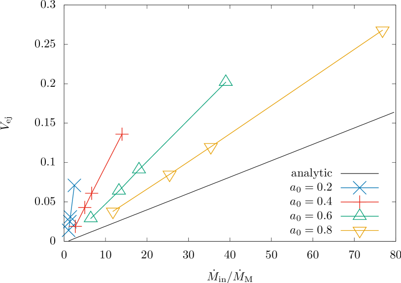
Figure 16: Maximum velocity attained by the ejected material $V_{\mathrm{ej}}$ as a function of the injection mass rate. The injection radius is $\mathcal{R}=100M$. The different symbols correspond to the numerical results reported in Tables 3–6 for $\gamma=5/3$ and sound speeds as labeled. The solid line corresponds to the analytic model of an ultrarelativistic $\gamma=2$ stiff fluid presented in Section 2.

4.2 Applicability in astrophysics

We discuss now the viability of the choked accretion phenomenon presented here for operating as the inner engine behind a given jet-launching astrophysical system. Given that the characteristic length scale of this mechanism is given by $\mathcal{S}$, we can expect the physical size of the inner accretion disk (that we have associated with $\mathcal{R}$) to be larger than $\mathcal{S}$. In general, for an accretion disk around a black hole, we will have $\mathcal{R}=1-10M$ (the actual value will be a function of both the disk model and the black hole spin). On the other hand, from all of the simulations presented in this work, as well as those in Aguayo-Ortiz et al. (2019) for the non-relativistic case, we see that a robust lower limit for $\mathcal{S}$ is given by the corresponding Bondi radius $r_{\mathrm{B}}=M/a_{\infty}^{2}$. Moreover, provided that $\mathcal{R}>r_{\mathrm{B}}$, we have $a_{0}\simeq a_{\infty}$ and then we can write

$$\mathcal{S}>M/a_{0}^{2}.$$ (4.1)

At this point it is useful to recall that, assuming an ideal gas, we can relate the sound speed $a$ and the fluid temperature $T$ by

$$\frac{T}{T_{i}}=\left(\frac{\gamma-1}{\gamma}\right)\left(\frac{a^{2}}{\gamma-1-a^{2}}\right),$$ (4.2)

where $T_{i}=m_{i}/k_{B}$ is the temperature corresponding to the rest mass energy of the average gas particle of mass $m_{i}$. For a gas composed of ionized hydrogen we have $T_{H}=1.08\times 10^{13}\,\mathrm{K}$, while for an electron-positron plasma $T_{e}=5.93\times 10^{9}\,\mathrm{K}$.

Then, from Eqs. (4.1) and (4.2) we have

$$\frac{\mathcal{S}}{M}>\frac{1}{\gamma}\frac{T_{i}}{T}+\frac{1}{\gamma-1}.$$ (4.3)

A regular plasma dominated by radiation pressure and consisting of protons and electrons can be modeled, in a first approximation, as a $\gamma=4/3$ polytrope with an average particle mass $m_{i}\simeq m_{H}$ and, thus, $T_{i}\simeq T_{H}$. As discussed in Aguayo-Ortiz et al. (2019), taking $T=10^{7}\,\mathrm{K}$ as the temperature at the inner edge of the disk in an X-ray binary (Kaaret et al., 2017), from Eq. (4.3) we have $\mathcal{S}>10^{5}M$. In the case of an AGN, instead of taking the gas in the inner disk (at a temperature of around $T=10^{5}\,\mathrm{K}$) we can consider the ionized plasma in the hot corona above the disk with a temperature of up to $T=10^{9}\,\mathrm{K}$  (Czerny et al., 2003). Nevertheless, even for this large temperature, from Eq. (4.3) we obtain $\mathcal{S}>10^{3}M$. Even in the case of the accretion disk associated to a long GRB, where the gas temperature can reach up to $10^{11}\,\mathrm{K}$ (Woosley, 1993), from Eq. (4.3) we have $\mathcal{S}>80M$, which is still a factor of ten larger than the expected size of the inner engine.

The above analysis implies that, for the choked accretion mechanism to work for a regular plasma, the temperature of the infalling gas is required to be substantially higher than that of the inferred values at the inner edge of the disk (or disk corona). These higher temperatures could result from highly localized heating processes such as magnetic reconnection, shock heating, or viscous friction at the point of transition between the disk and the radial-infall domains.

On the other hand, the extreme conditions at the innermost part of these systems give rise to a different kind of plasma composed of relativistic electron-positron pairs (Wardle et al., 1998; Beloborodov, 1999; Siegert et al., 2016). Considering that at least a fraction of this plasma has a thermal component, the pair production mechanism implies temperatures in excess of $10^{11}\,\mathrm{K}$. If we consider this gas as the accreted material, then for this temperature and substituting $T_{i}=T_{e}$ in Eq. (4.3), we get $\mathcal{S}>M$. We obtain then that, under these circumstances, the choked accretion mechanism might become relevant for the ejection of this pair plasma.

Contrary to the analytic model presented in Section 2, we do not have direct control on the mass injection rate crossing the outer boundary of our numerical simulations, as it is indirectly determined by the values of $\mathcal{R}$, $a_{0}$ and $\delta$. Nevertheless, it is clear that in an astrophysical scenario this mass rate will be imposed by external, possibly time varying conditions. For example, in the context of low mass X-ray binaries, stellar oscillations or orbital variations can modulate the total mass transfer across the Roche lobe from the regular star to the compact companion (Tauris & van den Heuvel, 2006). More dramatic time varying conditions will be found for jets launched during a common-envelope phase as studied by López-Cámara et al. (2019), or for long GRBs as studied by e.g. López-Cámara et al. (2010); Taylor et al. (2011).

The strong dependence that we have found between the ratio of ejected to injected material and the incoming mass accretion rate, leads us to suggest that the choked accretion mechanism could offer a compelling, simple connection between the external mass flux feeding an accretion disk and the jet activity. Whenever the mass injection rate surpasses the threshold value $\dot{M}_{\mathrm{M}}$, the excess flux is prone to being ejected from the system as a bipolar outflow. This could be of relevance for studying the time variability of the jet emission.

Once a tight connection appears between accretion rates and geometry on the one hand, and ejection rates and velocities on the other, we have the potential to correlate the time-variability in the mass flux across the accretion disk to the resulting ejection rates and velocities. This, in turn, naturally leads to the appearance of internal shocks in the ensuing jets, such as those typically assumed to be associated to the GRB phenomenology.

As already implied by the above discussion, a proper exploration of the role played by choked accretion in launching relativistic jets, demands accounting for additional physics, such as the effect of rotation, magnetic fields, and radiative transport. Indeed, these factors are considered as crucial for the acceleration and collimation of the resulting jets (Semenov et al., 2004; McKinney, 2006). Moreover, as discussed in Aguayo-Ortiz et al. (2019), some of these ingredients might actually improve the applicability of choked accretion by increasing both the effective temperature and the polar density contrast, thus bringing $\mathcal{S}$ closer to the central accretor. It should also be interesting to study the possible interplay of choked accretion with the well-established Blandford & Znajek (1977) mechanism. We intend to address these points in future work.

5 Summary

We have presented the choked accretion phenomenon as a purely hydrodynamical outflow-generating mechanism. Choked accretion operates under two basic premises: a sufficiently large mass flux accreting onto a central object, and an anisotropic density field in which an equatorial belt has a higher density than the polar regions. These two ingredients are plausibly met in several jet-launching astrophysical scenarios involving accretion discs around massive objects. We suggest that choked accretion constitutes a relevant ingredient for studying some of these systems.

Moreover, we have shown that breaking spherical symmetry by imposing a polar density gradient in the accretion flow onto a central object, qualitatively changes the resulting steady state configurations from the purely radial accretion models (Bondi, 1952; Michel, 1972), to the infall-outflow morphology that characterizes the choked accretion model. Thus, choked accretion provides a natural transition between spherical accretion and systems characterized by bipolar outflows.

We have studied this phenomenon by introducing first a general relativistic analytic model of choked accretion onto a Schwarzschild black hole. This model is based on the approximations of steady state, axisymmetry, and irrotational flow and assumes an ultrarelativistic stiff fluid. We then relaxed this last assumption, together with the associated potential flow condition, and studied more general fluids by means of full-hydrodynamic simulations performed with the numerical code aztekas.

Both for an ultrarelativistic stiff fluid as for a regular polytrope, the limiting value for the total mass accretion rate corresponds quite closely to the one found in the spherically-symmetric case (Michel, 1972). We have thus found that, within the assumptions underlying this work, hydrodynamical accretion flows onto massive objects choke at this threshold value and any extra infalling material is deflected into a bipolar outflow.

The analytic solution presented here allowed us to study in detail the basic physical principle behind the choked accretion phenomenon. Moreover, we have also demonstrated the usefulness of this exact analytic solution as a benchmark test for validating numerical hydrodynamic codes in general. The non-relativistic limit of this analytic solution is presented in Aguayo-Ortiz et al. (2019).

Considering together: i) the perturbative Newtonian solutions for isothermal fluids of  Hernandez et al. (2014); ii) the exact Newtonian solution for incompressible fluids and the numerical Newtonian experiments for polytropic equations of state in Aguayo-Ortiz et al. (2019); and iii) the present exact analytic relativistic model for a stiff fluid and the numerical experiments presented for polytropic fluids; we can conclude that the inflow-outflow steady state configurations presented here are an extremely general and robust consequence of breaking spherical symmetry with a polar density gradient in an accretion flow onto a central object. Similarly, we see that the choked accretion character of these configurations extends across the Newtonian and relativistic regimes.

Appendix A Relativistic, spherically symmetric accretion flow

In this Appendix we give a brief overview of Michel (1972)’s analytic model of a spherically symmetric accretion flow onto a Schwarzschild black hole. In particular we derive an analytic expression for the resulting mass accretion rate in a form that is useful for the present work (see Beskin & Pidoprygora, 1995, for an alternative derivation).

Here we will consider only the case of a perfect fluid described by a polytropic equation of state as in Eq. (3.1). See Chaverra & Sarbach (2015) for a recent extension of Michel (1972)’s model to a general class of static, spherically symmetric background metrics, as well as for more general equations of state.

Under the assumptions of stationary state and spherical symmetry, the equations governing the accretion flow are the continuity equation and the radial component of the relativistic Euler equation (Eqs. 2.4 and 2.5, respectively), i.e.

$$\frac{\mathrm{d}}{\mathrm{d}r}\left(r^{2}\rho\,U^{r}\right)=0,$$ (A.1)

$$\frac{\mathrm{d}}{\mathrm{d}r}\left(r^{2}T^{r}_{t}\right)=0,$$ (A.2)

where $v=U^{r}=\mathrm{d}r/\mathrm{d}\tau$ and $T^{r}_{t}=\rho\,h\,U_{t}\,U^{r}$. Direct integration of these two equations gives

$$4\pi\,r^{2}\rho\,v=\dot{M}_{\mathrm{M}}=4\pi\,\lambda=\mathrm{const.},$$ (A.3)

$$\rho\,h\,U_{t}\,v\,r^{2}=\mu=\mathrm{const.}$$ (A.4)

We can simplify Eq. (A.4) by dividing it by Eq. (A.3) and taking its square; the result is

$$h^{2}\left(1-\frac{2M}{r}+v^{2}\right)=\left(\frac{\mu}{\lambda}\right)^{2}=h^{2}_{\infty}.$$ (A.5)

Following Michel (1972), we can combine Eqs. (A.1) and (A.2) into the following differential equation

$$\begin{split}\bigg{[}1-\frac{a^{2}}{v^{2}}\bigg{(}1&-\frac{2M}{r}+v^{2}\bigg{)}\bigg{]}v\frac{\mathrm{d}v}{\mathrm{d}r}=\\ &-\frac{M}{r^{2}}+2\,\frac{a^{2}}{r}\left(1-\frac{2M}{r}+v^{2}\right).\end{split}$$ (A.6)

From Eq. (A.6) we obtain that the condition of having a critical point, i.e. a radius $r=r_{c}$ at which both sides of this equation vanish simultaneously, translates into

$$v_{c}^{2}=\frac{1}{2}\,\frac{M}{r_{c}},$$ (A.7)

and

$$a_{c}^{2}=\frac{v_{c}^{2}}{1-3\,v_{c}^{2}}.$$ (A.8)

Substituting Eqs. (A.7) and (A.8) into Eq. (A.5) results in

$$n\,h_{c}^{3}-h^{2}_{\infty}\left[(n+3)h_{c}-3\right]=0,$$ (A.9)

where $n=1/(\gamma-1)$. This polynomial has three real roots for $h_{c}$, but only one satisfies $h_{c}>1$ and thus has physical meaning. This root is given by

$$h_{c}=2\,h_{\infty}\,\sqrt{\frac{n+3}{3\,n}}\,\sin\left(\Psi+\frac{\pi}{6}\right),$$ (A.10)

where

$$\cos(3\,\Psi)=\frac{3}{2\,n\,h_{\infty}}\left(\frac{n+3}{3\,n}\right)^{-3/2}.$$ (A.11)

We can now find an expression for the accretion rate in terms of $M$, the equation of state of the fluid, and its asymptotic conditions (expressed in terms of $\rho_{\infty}$ and $h_{\infty}$). Let us start by substituting Eq. (A.7) into the continuity equation (A.3), which results in

$$\lambda=r_{c}^{2}\,\rho_{c}\,v_{c}=\frac{1}{4}\,M^{2}\rho_{c}\,v_{c}^{-3}.$$ (A.12)

Now, using Eqs. (3.1) and (3.3), we can rewrite the equation of state as

$$\rho_{c}=\rho_{\infty}\left(\frac{h_{c}-1}{h_{\infty}-1}\right)^{n},$$ (A.13)

on the other hand, by combining Eqs. (3.4), (A.8) and (A.10) we obtain

$$v_{c}^{2}=\frac{h_{c}-1}{(n+3)h_{c}-3}=\frac{h^{2}_{\infty}(h_{c}-1)}{n\,h^{3}_{c}}.$$ (A.14)

Then, substituting Eqs. (A.13) and (A.14) into Eq. (A.12) we obtain

$$\dot{M}_{\mathrm{M}}=4\pi\,\lambda=\pi\left[\frac{n^{3}h_{c}^{9}}{h^{6}_{\infty}}\frac{(h_{c}-1)^{2n-3}}{(h_{\infty}-1)^{2n}}\right]^{1/2}M^{2}\rho_{\infty}.$$ (A.15)

Note that $\dot{M}_{\mathrm{M}}$ as expressed in Eq. (A.15) is given in terms of thermodynamical quantities measured asymptotically far away from the central object ($\rho_{\infty}$ and either $a_{\infty}$ or $h_{\infty}$). In order to compare the results presented in Section 2 with Michel’s solution, one needs first to find the asymptotic values $\rho_{\infty}$ and $a_{\infty}$ resulting in a solution such that $\rho|_{\mathcal{R}}=\rho_{0}$ and $a|_{\mathcal{R}}=a_{0}$.

Appendix B Validation of the numerical code

In this appendix, we present a series of standard tests in order to validate the results using aztekas. This section is complementary to the test already presented in Section 3.1 as well as the appendix presented in Tejeda & Aguayo-Ortiz (2019), where the code is tested using the relativistic spherical accretion problem (Michel, 1972).

B.1 One-dimensional shock tube tests

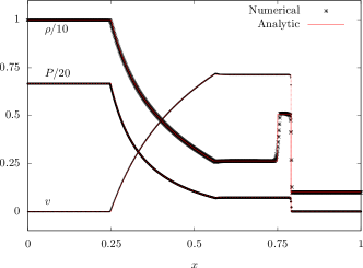
(a) Test 1

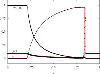
(b) Test 2

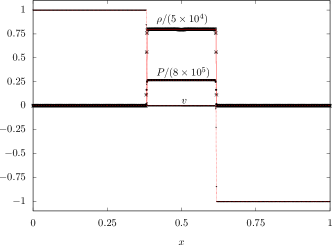
(c) Test 3

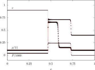
(d) Test 4

Figure B.1: Evolution at a time $t=0.35$ of the density $\rho$, pressure $P$ and velocity $v$ for the four tests presented in Table B.1. All tests were performed using a resolution $N=800$ with a Courant factor of 0.5.

The one-dimensional shock tube test (Sod, 1978) is a standard problem to solve for code validation, as it is easy to implement and the exact solution can be computed. It consists of a perfect fluid at two different initial states with parameters $(\rho_{L},P_{L},v_{L})$ and $(\rho_{R},P_{R},v_{R})$ (where subscripts $L$ and $R$ refer to the left and right sides, respectively), separated by an interface at $x=x_{0}$. At $t=0$ the interface is removed and the two states are left to interact with each other. The evolution of this configuration depends only on the initial values and on the equation of state. Here we present a set of four one-dimensional shock tube tests, along with a two-dimensional version of the problem. For the former case, we compare the results with the analytic solution.

We reproduce four of the shock tube tests presented by Lora-Clavijo et al. (2015). The tests were performed in a Cartesian 1D domain $x\in[0,1]$ with a resolution $N=800$ and a Courant number of 0.5. The initial conditions of each test are presented in Table B.1. Test 1 and Test 2 correspond to a midly and strong relativistic blast wave explosion, respectively. The initial conditions for Test 3 produce a highly relativistic symmetric head-on stream collision, with a Lorentz factor $\Gamma=1000$. Finally, Test 4 follows the evolution of a shock travelling at $v=0.9$, as seen from the rest frame of the shock front.

Table B.1: Initial conditions for the left $(L)$ and right $(R)$ states of the set of one-dimensional shock tube tests.

	Test 1	Test 2	Test 3	Test 4
$\rho_{L}$	10	1	1	1
$P_{L}$	13.33	1000	0.001	1
$v_{L}$	0	0	0.999999995	0.9
$\rho_{R}$	1	1	1	1
$P_{R}$	$10^{-8}$	0.001	0.001	10
$v_{R}$	0	0	-0.999999995	0
$\gamma$	5/3	5/3	4/3	4/3

In Figure B.1 we show the evolution of all four tests at $t=0.35$ and the comparison between the numerical simulations performed with aztekas and the analytic solution. The latter was computed using a code written by Martí & Müller (1999). In the first two tests, a contact discontinuity and a rarefaction wave are formed. In Test 1, where the Lorentz factor is $\Gamma\approx 1$ the analytic solution is well resolved. In Test 2, where the Lorentz factor is $\Gamma\approx 6$, we obtain an overall satisfactory result although a higher resolution should lead to a better defined contact discontinuity. Test 3 shows the evolution of a strong head-on collision between two shock waves. A stationary high density, high pressure shell is formed and we see again a good match with the analytic solution. Finally, in Test 4, we can see the formation of a stationary contact discontinuity. In this case small oscillations are developed right behind the shock. This oscillations are damped with higher resolution. All the results presented here agree with previous works that use similar schemes (e.g. Lucas-Serrano et al., 2004; De Colle et al., 2012; Lora-Clavijo et al., 2015).

B.2 Two-dimensional Riemann problem

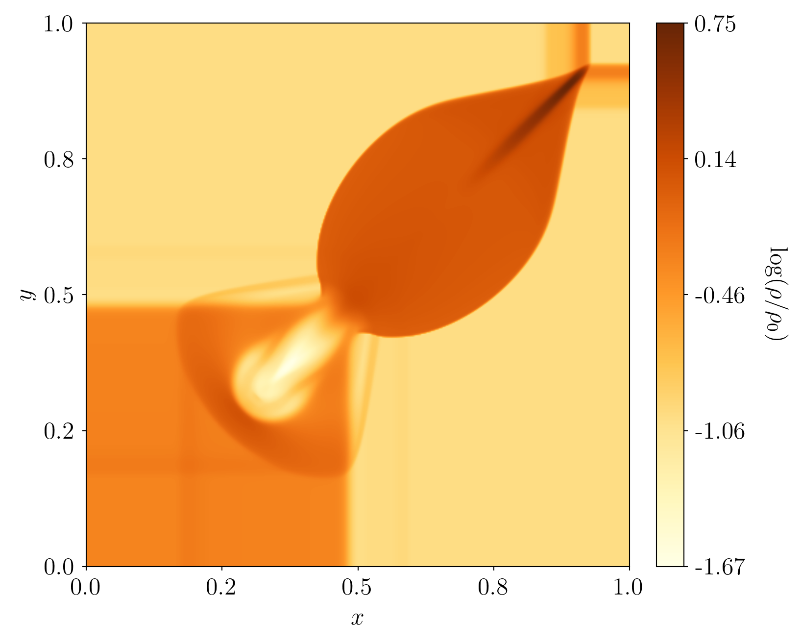
Figure B.2: Logarithmic rest mass density colour map of the two-dimensional Riemann problem at a time $t=0.4$. The simulation was performed using a $400\times 400$ resolution and a Courant factor of 0.25.

For this test, we follow closely the initial setup proposed by Del Zanna & Bucciantini (2002) for the two-dimensional Riemann problem, which is the relativistic extension of the case presented by (Lax & Liu, 1998). The problem consists on a square domain subdivided into four regions with different initial states

$$\footnotesize(\rho,P,v_{x},v_{y})=\left\{\begin{split}(0.1,0.01,0,0)\quad&\mathrm{if}\quad x>0.5\text{,}\,\,\,y>0.5,\\ (0.1,1,0.99,0)\quad&\mathrm{if}\quad x\leq 0.5\text{,}\,\,\,y>0.5,\\ (0.5,1,0,0)\,\,\,\,\,\,\,\,\quad&\mathrm{if}\quad x>0.5\text{,}\,\,\,y\leq 0.5,\\ (0.1,1,0,0.99)\quad&\mathrm{if}\quad x\leq 0.5\text{,}\,\,\,y\leq 0.5.\end{split}\right.$$ (B.1)

The test was performed in a 2D Cartesian domain $(x,y)\in[0,1]\times[0,1]$ with a $400\times 400$ resolution and a Courant number of 0.25. In Figure B.2 we show the evolution of the rest mass density at a time $t=0.4$. The morphology of the solution shows a stationary high density contact discontinuity along the diagonal of the domain, and a jet-like structure propagating into the initially over-dense region. This results are qualitatively similar to the ones obtained by Del Zanna & Bucciantini (2002); De Colle et al. (2012); Lora-Clavijo et al. (2015).

References

- Abbott et al. (2017) Abbott, B. P., Abbott, R., Abbott, T. D., et al. 2017, Physical Review Letters, 119, 161101, doi: 10.1103/PhysRevLett.119.161101
- Aguayo-Ortiz et al. (2018) Aguayo-Ortiz, A., Mendoza, S., & Olvera, D. 2018, PLoS ONE, 13, e0195494, doi: 10.1371/journal.pone.0195494
- Aguayo-Ortiz et al. (2019) Aguayo-Ortiz, A., Tejeda, E., & Hernandez, X. 2019, Monthly Notices of the Royal Astronomical Society, 490, 5078, doi: 10.1093/mnras/stz2989
- Balbus & Hawley (1991) Balbus, S. A., & Hawley, J. F. 1991, Astrophysical Journal, 376, 214, doi: 10.1086/170270
- Banyuls et al. (1997) Banyuls, F., Font, J. A., Ibáñez, J. M., Martí, J. M., & Miralles, J. A. 1997, Astrophysical Journal, 476, 221, doi: 10.1086/303604
- Beckmann & Shrader (2012) Beckmann, V., & Shrader, C. R. 2012, Active Galactic Nuclei
- Beloborodov (1999) Beloborodov, A. M. 1999, Monthly Notices of the Royal Astronomical Society, 305, 181, doi: 10.1046/j.1365-8711.1999.02384.x
- Beskin & Pidoprygora (1995) Beskin, V. S., & Pidoprygora, Y. N. 1995, Soviet Journal of Experimental and Theoretical Physics, 80, 575
- Blandford et al. (2019) Blandford, R., Meier, D., & Readhead, A. 2019, ARA&A, 57, 467, doi: 10.1146/annurev-astro-081817-051948
- Blandford & Payne (1982) Blandford, R. D., & Payne, D. G. 1982, Monthly Notices of the Royal Astronomical Society, 199, 883, doi: 10.1093/mnras/199.4.883
- Blandford & Znajek (1977) Blandford, R. D., & Znajek, R. L. 1977, Monthly Notices of the Royal Astronomical Society, 179, 433, doi: 10.1093/mnras/179.3.433
- Bondi (1952) Bondi, H. 1952, Monthly Notices of the Royal Astronomical Society, 112, 195+
- Burrows et al. (2011) Burrows, D. N., Kennea, J. A., Ghisellini, G., et al. 2011, Nature, 476, 421, doi: 10.1038/nature10374
- Chaverra & Sarbach (2015) Chaverra, E., & Sarbach, O. 2015, Classical and Quantum Gravity, 32, 155006, doi: 10.1088/0264-9381/32/15/155006
- Czerny et al. (2003) Czerny, B., Nikołajuk, M., Różańska, A., et al. 2003, A&A, 412, 317, doi: 10.1051/0004-6361:20031441
- De Colle et al. (2012) De Colle, F., Granot, J., López-Cámara, D., & Ramirez-Ruiz, E. 2012, ApJ, 746, 122, doi: 10.1088/0004-637X/746/2/122
- Del Zanna & Bucciantini (2002) Del Zanna, L., & Bucciantini, N. 2002, A&A, 390, 1177, doi: 10.1051/0004-6361:20020776
- Fendt (2018) Fendt, C. 2018, Contributions of the Astronomical Observatory Skalnate Pleso, 48, 40
- Hartigan (2009) Hartigan, P. 2009, Astrophysics and Space Science Proceedings, 13, 317, doi: 10.1007/978-3-642-00576-3_38
- Hawley et al. (2015) Hawley, J. F., Fendt, C., Hardcastle, M., Nokhrina, E., & Tchekhovskoy, A. 2015, Space Sci. Rev., 191, 441, doi: 10.1007/s11214-015-0174-7
- Hernandez et al. (2014) Hernandez, X., Rendón, P. L., Rodríguez-Mota, R. G., & Capella, A. 2014, Revista Mexicana de Astronomía y Astrofísica, 50, 23. https://arxiv.org/abs/1103.0250
- Kaaret et al. (2017) Kaaret, P., Feng, H., & Roberts, T. P. 2017, ARA&A, 55, 303, doi: 10.1146/annurev-astro-091916-055259
- Komissarov et al. (2007) Komissarov, S. S., Barkov, M. V., Vlahakis, N., & Königl, A. 2007, Monthly Notices of the Royal Astronomical Society, 380, 51, doi: 10.1111/j.1365-2966.2007.12050.x
- Lattimer & Prakash (2007) Lattimer, J. M., & Prakash, M. 2007, Phys. Rep., 442, 109, doi: 10.1016/j.physrep.2007.02.003
- Lax & Liu (1998) Lax, P. D., & Liu, X.-D. 1998, SIAM Journal on Scientific Computing, 19, 319, doi: 10.1137/S1064827595291819
- Liska et al. (2019) Liska, M., Tchekhovskoy, A., Ingram, A., & van der Klis, M. 2019, Monthly Notices of the Royal Astronomical Society, 487, 550, doi: 10.1093/mnras/stz834
- Lloyd-Ronning et al. (2019) Lloyd-Ronning, N. M., Fryer, C., Miller, J. M., et al. 2019, MNRAS, 485, 203, doi: 10.1093/mnras/stz390
- López-Cámara et al. (2019) López-Cámara, D., De Colle, F., & Moreno Méndez, E. 2019, Monthly Notices of the Royal Astronomical Society, 482, 3646, doi: 10.1093/mnras/sty2959
- López-Cámara et al. (2010) López-Cámara, D., Lee, W. H., & Ramirez-Ruiz, E. 2010, Astrophysical Journal, 716, 1308, doi: 10.1088/0004-637X/716/2/1308
- Lora-Clavijo et al. (2015) Lora-Clavijo, F. D., Cruz-Osorio, A., & Guzmán, F. S. 2015, ApJS, 218, 24, doi: 10.1088/0067-0049/218/2/24
- Lucas-Serrano et al. (2004) Lucas-Serrano, A., Font, J. A., Ibáñez, J. M., & Martí, J. M. 2004, A&A, 428, 703, doi: 10.1051/0004-6361:20035731
- Martí & Müller (1999) Martí, J. M., & Müller, E. 1999, Living Reviews in Relativity, 2, 3, doi: 10.12942/lrr-1999-3
- McKinney (2006) McKinney, J. C. 2006, Monthly Notices of the Royal Astronomical Society, 368, 1561, doi: 10.1111/j.1365-2966.2006.10256.x
- Michel (1972) Michel, F. C. 1972, Astrophysics and Space Science, 15, 153
- Mirabel & Rodríguez (1994) Mirabel, I. F., & Rodríguez, L. F. 1994, Nature, 371, 46, doi: 10.1038/371046a0
- Moncrief (1980) Moncrief, V. 1980, Astrophysical Journal, 235, 1038, doi: 10.1086/157707
- Olvera & Mendoza (2008) Olvera, D., & Mendoza, S. 2008, in EAS Publications Series, Vol. 30, EAS Publications Series, ed. A. Oscoz, E. Mediavilla, & M. Serra-Ricart, 399–400, doi: 10.1051/eas:0830072
- Ouyed et al. (2003) Ouyed, R., Clarke, D. A., & Pudritz, R. E. 2003, ApJ, 582, 292, doi: 10.1086/344507
- Petrich et al. (1988) Petrich, L. I., Shapiro, S. L., & Teukolsky, S. A. 1988, Physical Review Letters, 60, 1781, doi: 10.1103/PhysRevLett.60.1781
- Pudritz et al. (2007) Pudritz, R. E., Ouyed, R., Fendt, C., & Brandenburg, A. 2007, in Protostars and Planets V, ed. B. Reipurth, D. Jewitt, & K. Keil, 277. https://arxiv.org/abs/astro-ph/0603592
- Qian et al. (2018) Qian, Q., Fendt, C., & Vourellis, C. 2018, Astrophysical Journal, 859, 28, doi: 10.3847/1538-4357/aabd36
- Romero et al. (2017) Romero, G. E., Boettcher, M., Markoff, S., & Tavecchio, F. 2017, Space Sci. Rev., 207, 5, doi: 10.1007/s11214-016-0328-2
- Semenov et al. (2004) Semenov, V., Dyadechkin, S., & Punsly, B. 2004, Science, 305, 978, doi: 10.1126/science.1100638
- Shakura & Sunyaev (1973) Shakura, N. I., & Sunyaev, R. A. 1973, Astronomy and Astrophysics, 24, 337
- Shu & Osher (1988) Shu, C.-W., & Osher, S. 1988, Journal of Computational Physics, 77, 439, doi: 10.1016/0021-9991(88)90177-5
- Siegert et al. (2016) Siegert, T., Diehl, R., Greiner, J., et al. 2016, Nature, 531, 341, doi: 10.1038/nature16978
- Sod (1978) Sod, G. A. 1978, Journal of Computational Physics, 27, 1, doi: 10.1016/0021-9991(78)90023-2
- Tauris & van den Heuvel (2006) Tauris, T. M., & van den Heuvel, E. P. J. 2006, Formation and evolution of compact stellar X-ray sources, Vol. 39, 623–665
- Taylor et al. (2011) Taylor, P. A., Miller, J. C., & Podsiadlowski, P. 2011, Monthly Notices of the Royal Astronomical Society, 410, 2385, doi: 10.1111/j.1365-2966.2010.17618.x
- Tejeda (2018) Tejeda, E. 2018, Revista Mexicana de Astronomía y Astrofísica, 54, 171. https://arxiv.org/abs/1705.07093
- Tejeda & Aguayo-Ortiz (2019) Tejeda, E., & Aguayo-Ortiz, A. 2019, Monthly Notices of the Royal Astronomical Society, 487, 3607, doi: 10.1093/mnras/stz1513
- Wardle et al. (1998) Wardle, J. F. C., Homan, D. C., Ojha, R., & Roberts, D. H. 1998, Nature, 395, 457, doi: 10.1038/26675
- Waters et al. (2020) Waters, T., Aykutalp, A., Proga, D., et al. 2020, Monthly Notices of the Royal Astronomical Society, 491, L76, doi: 10.1093/mnrasl/slz168
- Woosley (1993) Woosley, S. E. 1993, in Bulletin of the American Astronomical Society, Vol. 25, American Astronomical Society Meeting Abstracts #182, 894
- Woosley & Bloom (2006) Woosley, S. E., & Bloom, J. S. 2006, Annual Review of Astronomy and Astrophysics, 44, 507, doi: 10.1146/annurev.astro.43.072103.150558
- Zahra Zeraatgari et al. (2020) Zahra Zeraatgari, F., Mosallanezhad, A., Yuan, Y.-F., Bu, D.-F., & Mei, L. 2020, ApJ, 888, 86, doi: 10.3847/1538-4357/ab594f
- Zhong et al. (2019) Zhong, S.-Q., Dai, Z.-G., & Deng, C.-M. 2019, ApJ, 883, L19, doi: 10.3847/2041-8213/ab40c5