Deep Esophageal Clinical Target Volume Delineation using Encoded 3D Spatial Context of Tumors, Lymph Nodes, and Organs At Risk

Abstract

CTV delineation from RTCT images is used to define the treatment areas containing the GTV and/or sub-clinical malignant disease for RT. High intra- and inter-user variability makes this a particularly difficult task for esophageal cancer. This motivates automated solutions, which is the aim of our work. Because CTV delineation is highly context-dependent—it must encompass the GTV and regional LN while also avoiding excessive exposure to the OAR—we formulate it as a deep contextual appearance-based problem using encoded spatial contexts of these anatomical structures. This allows the deep network to better learn from and emulate the margin- and appearance-based delineation performed by human physicians. Additionally, we develop domain-specific data augmentation to inject robustness to our system. Finally, we show that a simple 3D PHNN, which avoids computationally heavy decoding paths while still aggregating features at different levels of context, can outperform more complicated networks. Cross-validated experiments on a dataset of $135$ esophageal cancer patients demonstrate that our encoded spatial context approach can produce concrete performance improvements, with an average Dice score of $83.9\pm 5.4\%$ and an average surface distance of $4.2\pm 2.7\,\mathrm{mm}$, representing improvements of $3.8\%$ and $2.4\mathrm{mm}$, respectively, over the state-of-the-art approach.

1 Introduction

Esophageal cancer ranks the sixth in global cancer mortality [1]. As it is usually diagnosed at rather late stage [18], RT is a cornerstone of treatment. Delineating the 3D CTV on a RTCT scan is a key challenge in RT planning. As Fig. 1 illustrates, the CTV should spatially encompass, with a mixture of predefined and judgment-based margins, primary tumor(s), i.e., the GTV, regional LN and sub-clinical disease regions, while simultaneously limiting radiation exposure to OAR [2].

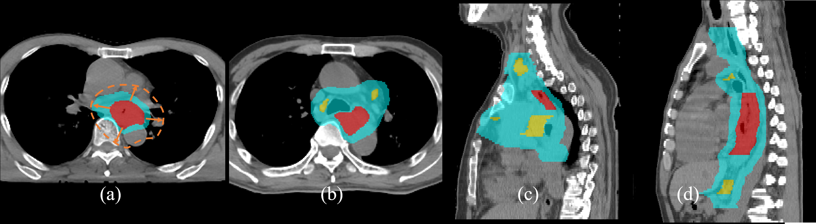
Figure 1: Esophageal cancer CTV delineation, where red, yellow, and cyan indicate the GTV, regional LN and CTV, respectively. (a) shows that the CTV is not a uniform margin expansion (brown-dotted line) from the GTV, while (b)-(d) shows how delineation becomes more complicated when regional LN are present. (c) and (d) also depict wide and long examples of esophageal CTV, respectively.

Esophageal CTV delineation is uniquely challenging because tumors may potentially spread along the entire esophagus and metastasize up to the neck or down to the upper abdomen LN. Current clinical protocols rely on manual CTV delineation, which is very time and labor consuming and is subject to high inter- and intra-observer variability [12]. This motivates automated approaches to the CTV delineation.

Deep CNN have achieved notable successes in segmenting semantic objects, such as organs and tumors, in medical imaging [4, 9, 6, 10, 7, 8]. However, to the best of our knowledge, no prior work, CNN-based or not, has addressed esophageal cancer CTV segmentation. Works on CTV segmentation of other cancer types mostly operate based on the RTCT appearance alone [14, 15]. As shown in Fig. 1, CTV delineation depends on the radiation oncologist’s visual judgment of both the appearance and the spatial configuration of the GTV, LN, and OAR, suggesting that only considering the RTCT makes the problem ill-posed. Supporting this, Cardenas et al. recently showed that considering the GTV and LN binary masks together with the RTCT can boost oropharyngeal CTV delineation performance [3]. However, the OAR were not considered in their work. Moreover, binary masks do not explicitly provide distances to the model. Yet CTV delineation is highly driven by distance-based margins to other anatomical structures of interest, and it is difficult to see how regular CNN could capture these precise distance relationships with binary masks alone.

Our work fills this gap by introducing a spatial-context encoded deep CTV delineation framework. Instead of expecting the CNN to learn distance-based margins from the GTV, LN, and OAR binary masks, we provide the CTV delineation network with the 3D SDT [16] of these structures. Specifically, we include the SDT of the GTV, LN, lung, heart, and spinal canal with the original RTCT volume as inputs to the network. From a clinical perspective, this allows the CNN to emulate the oncologist’s manual delineation, which uses the distances of GTV and LN vs. the OAR as a key constraint in determining CTV boundaries. To improve robustness, we randomly choose manually and automatically generated OAR SDT during training, while augmenting the GTV and LN SDT with the domain-specific jittering. We adopt a 3D PHNN [6] to serve as our delineation model, which enjoys the benefits of strong abstraction capacities and multi-scale feature fusion with a light-weighted decoding path. We extensively evaluate our approach using a 3-fold cross-validated dataset of $135$ esophageal cancer patients. Since we are the first to tackle automated esophageal cancer CTV delineation, we compare against previous CTV delineation methods for other cancers [15, 3], using the 3D PHNN as the delineation model. When comparing against pure appearance-based [15] and binary-mask-based [3] solutions, we show that our approach provides improvements of $10\%$ and $3.8\%$ in Dice score, respectively, with analogous improvements in HD and ASD. Moreover, we also show that PHNN is responsible for providing improvements of $1\%$ in Dice score and $0.4mm$ reduction in ASD over a 3D U-Net model [4].

2 Methods

CTV delineation in RT planning is essentially a margin expansion process, starting from observable tumorous regions (GTV and regional LN) and extending into the neighboring regions by considering the possible tumor spread margins and distances to nearby healthy OAR. Fig. 2 depicts an overview of our method, which consists of four major modularized components: (1) segmentation of prerequisite regions; (2) SDT computation; (3) domain-specific data augmentation; and (4) a 3D PHNN to execute the CTV delineation.

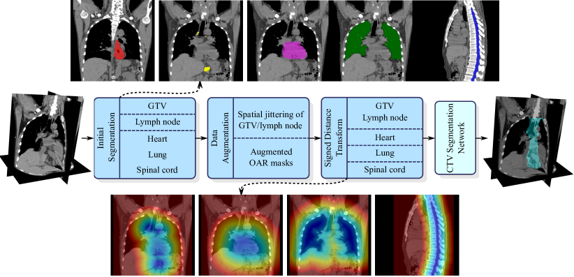
Figure 2: Overall workflow of our spatial context encoded CTV delineation framework. The top and bottom rows depict different masks and SDT, respectively, overlayed on the RTCT. From left to right are the GTV, LN, heart, lung, and spinal canal. The GTV and LN share a combined SDT.

2.1 Prerequisite Region Segmentation

To provide spatial context/distance of the anatomical structures of interest, we must first know their boundaries. We assume that manual segmentations for the esophageal GTV and regional LN are available. However, we do not make this assumption for the OAR. Indeed, missing OAR segmentations ($\sim 20\%$) is common in our dataset. For the OAR, we consider three major organs: the lung, heart, and spinal canal, since most esophageal CTV are closely integrated with these organs. Using the available organ labels, we trained a 2D PHNN [6] to segment the OAR, considering its robust performance in pathological lung segmentation and its computational efficiency. Examples of automatic OAR segmentation are illustrated in the first row in Fig. 2 and validation Dice score for the lung, heart and spinal canal were $97\%$, $95\%$ and $78\%$, respectively, in our dataset.

2.2 SDT Computation

To encode the spatial context with respect to the GTV, regional LN, and OAR, we compute SDT for each. The SDT is generated from a binary image, where the value in each voxel measures the distance to the closest object boundary. Voxels inside and outside the boundary have positive and negative values, respectively. More formally, let $\mathcal{O}_{i}$ denote a binary mask, where $i\in\{\text{GTV+LNs, lung, heart, spinal canal}\}$ and let $\Gamma(\cdot)$ be a function that computes boundary voxels of a binary image. The SDT value at a voxel $p$ with respect to $\mathcal{O}_{i}$ is computed as

$$\text{SDM}_{\Gamma(\mathcal{O}_{i})}(p)=\left\{\begin{array}[]{rcl}\underset{q\in\Gamma(\mathcal{O}_{i})}{\min}d(p,q)&\quad{\text{if}\quad p\notin\mathcal{O}_{i}}\\ -\underset{q\in\Gamma(\mathcal{O}_{i})}{\min}d(p,q)&\quad{\text{if}\quad p\in\mathcal{O}_{i}}\end{array}\right.\mathrm{,}$$ (3)

where $d(p,q)$ is a distance measure from $p$ to $q$. We choose to use Euclidean distance in our work and use Maurer et al.’s efficient algorithm [13] to compute the SDT. The bottom row in Fig. 2 depicts example SDT for the combined GTV and LN and the other 3 OAR. Note that we compute SDT separately for each of the three OAR, meaning we can capture each organ’s influence on the CTV. Providing the SDT of the GTV, LN, and OAR to the deep CNN allows it to more easily infer the distance-based margins to these anatomical structures, better emulating the oncologist’s CTV inference process.

2.3 Domain-Specific Data Augmentation

We adopt specialized data augmentations to increase the robustness of the training and harden our network to noise in the prerequisite segmentations. Specifically, two types of data augmentation are carried out. (1) We calculate the GTV and LN SDT from both the manual annotations and also spatially jittered versions of those annotations. We jitter each GTV and LN component by random shift within $4\times 4\times 4\,\mathrm{mm}^{3}$, mimicking that in practice $4\,\mathrm{mm}$ average distance error represents the state-of-the art performance in esophageal GTV segmentation [17, 8]. (2) We calculate SDT of the OAR using both the manual annotations and the automatic segmentations from §2.1. Combined, these augmentations lead to four possible combinations, which we randomly choose between during every training epoch. This increases model robustness and also allows the system to be effectively deployed in practice by using SDT of the automatically segmented OAR , helping to alleviate the labor involved.

2.4 CTV Delineation Network

To use 3D CNN in medical imaging, one has to strike a balance between choosing the appropriate image size covering enough context and the GPU memory. The symmetric encoder-decoder segmentation networks, e.g., 3D U-Net [4], are computationally heavy and memory-consuming since half of its computation is consumed on the decoding path, which may not always be needed for all 3D segmentation tasks. To alleviate the computational/memory burden, we adopt a 3D version of PHNN [6] as our CTV delineation network, which is able to fuse different levels of features using parameter-less deep supervision. We keep the first 4 convolutional blocks and adapt it to 3D as our network structure. As we demonstrate in the experiments, the 3D PHNN is not only able to achieve reasonable improvement over the 3D U-Net but requires 3 times less GPU memory.

3 Experiments and Results

To evaluate the performance of our esophageal CTV delineation framework, we collected from $135$ anonymized RTCT of esophageal cancer patients undergoing RT. Each RTCT is accompanied by a CTV mask annotated by an experienced oncologist, based on a previously segmented GTV, regional LN, and OAR. The average RTCT size is $512\times 512\times 250$ voxels with the average resolution of $1.05\times 1.05\times 2.6$ mm.

Training data sampling: We first resample all the CT and SDT images to a fixed resolution of $1.0\times 1.0\times 2.5$ mm, from which we extract $96\times 96\times 64$ training VOI patches in two manners: (1) To ensure enough VOI with positive CTV content, we randomly extract VOI centered within the CTV mask. (2) To obtain sufficient negative examples, we randomly sample $\sim 20$ VOI from the whole volume. This results in on average $80$ VOI per patient. We further augment the training data by applying random rotations of $\pm 10$ degrees in the x-y plane.

Implementation details: The Adam solver [11] is used to optimize all segmentation models with a momentum of $0.99$ and a weight decay of $0.005$ for $30$ epochs. We use the Dice loss for training. For testing, we use 3D sliding windows with sub-volumes of $96\times 96\times 64$ and strides of $64\times 64\times 32$ voxels. The probability maps of sub-volumes are aggregated to obtain the whole volume prediction taking on average $6-7\,\mathrm{s}$ to process one input volume using a Titan-V GPU.

Comparison setup and metrics: We use 3-fold cross-validation, separated at the patient level, to evaluate performance of our approach and the competitor methods. We compare against setups using only the CT appearance information [14, 15] and setups using the CT with binary GTV/LN masks [3]. Finally, we also compare against setups using the CT + GTV/LN SDT, which does not consider the OAR. We compare these setups using the 3D PHNN. For the 3D U-Net [4], we compared against the setup using the CT appearance information. We evaluate the performance using the metrics of Dice score, ASD and HD.

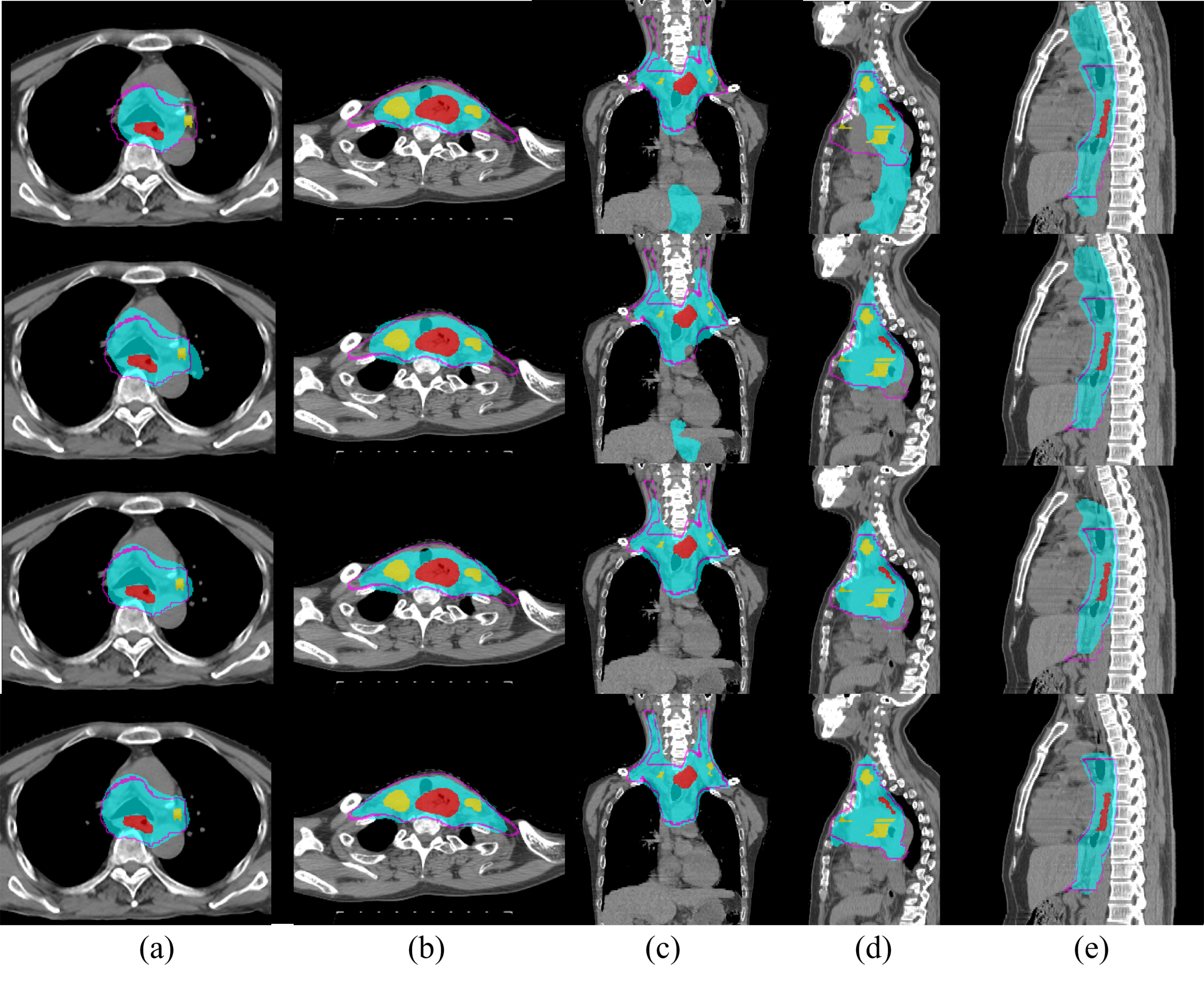
Figure 3: Qualitative illustration of esophageal CTV delineation using different PHNN setups. Red, yellow and cyan represent the GTV, LN and predicted CTV regions, respectively. The purple line indicates the ground truth CTV boundary. The $1^{st}$ and $2^{nd}$ rows show examples from setups using pure RTCT [15] and when adding GTV/LN binary masks [3], respectively. The $3^{rd}$ and $4^{th}$ row show examples when adding GTV/LN SDT and our proposed GTV/LN/OAR SDT, respectively. (a) and (d) demonstrate that the pure RTCT setups fail to include the regional LN, while (c) to (e) depict severe over-segmentations. While these errors are partially addressed using the GTV/LN mask setup, it still suffers from inaccurate CTV boundaries (a-c) or over coverage of normal regions (d,e). These issues are much better addressed by our proposed method.

Table 1: Quantitative results for the esophageal cancer CTV delineation. The last, starred row represents performance when using automatically generated OAR SDT.

Models	Setups	Dice	HD (mm)	ASD (mm)
U-Net	CT	0.739$\pm$0.126	69.5$\pm$42.7	10.1$\pm$9.4
	CT + GTV/LN/OAR SDT	0.829$\pm$0.061	36.9$\pm$23.8	4.6$\pm$3.0
PHNN	CT	0.739$\pm$0.117	68.5$\pm$43.8	10.6$\pm$9.2
	CT + GTV/LN masks	0.801$\pm$0.075	56.3$\pm$35.4	6.6$\pm$5.3
	CT + GTV/LN SDT	0.816$\pm$0.067	44.7$\pm$25.1	5.4$\pm$4.1
	CT + GTV/LN/OAR SDT	0.839$\pm$0.054	35.4$\pm$23.7	4.2$\pm$2.7
	CT + GTV/LN/OAR SDT*	0.823$\pm$0.059	43.6$\pm$26.4	5.1$\pm$3.3

Results: Table 1 outlines the quantitative comparisons of the different model setups and choices. As can be seen, methods based on pure CT appearance, seen in prior art [14, 15], exhibits the worst performance. This is because inferring distance-based margins from appearance alone is too hard of a task for CNN. Focusing on the PHNN performance, when adding the binary GTV and LN masks as contextual information [3], the performance increases considerably from $0.739\pm 0.117$ to $0.801\pm 0.075$ in Dice score. When using the SDT encoded spatial context of GTV/LN, PHNN further improves the Dice score and ASD by $1.5\%$ and $1.2\,\mathrm{mm}$, respectively, confirming the value of using the distance information for esophageal CTV delineation. Finally, when the OAR SDT are included, i.e., our proposed framework, PHNN achieves the best performance reaching $0.839\pm 0.054$ Dice score and $4.2\pm 2.7\,\mathrm{mm}$ ASD, with a reduction of $9.3\,\mathrm{mm}$ in HD as compared to the next best PHNN result. Fig. 4 depicts cumulative histograms of the Dice score and ASD, visually illustrating the distribution of improvements in the CTV delineation performance. Fig. 3 shows some qualitative examples illustrating these performance improvements. Interestingly, as the last row of Table 1 shows, when using SDT computed from the automatically segmented OAR for testing, the performance compares favorably to the best configuration, and outperforms all other configurations. This indicates that our method remains robust to noise within the OAR SDT and also that our approach is not reliant on manual OAR masks for good performance, increasing its practical value.

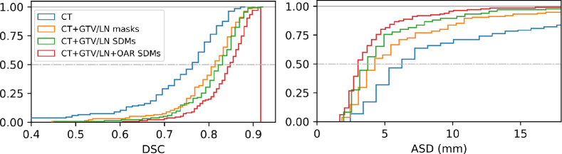
Figure 4: Cumulative histograms of the CTV delineation performance under 4 setups using 3D PHNN on cross-validated 135 patients. The left and right depict the Dice score and ASD results, respectively. From the results, we observe that $>77\%$ patients have Dice score $\geq 0.80$, and $>55\%$ patients have Dice score $\geq 0.85$ by using the proposed method (shown in red). Since there are often large inter-observer variations on CVT delineation tasks, i.e., ranging from 0.51 to 0.81 in terms of Jaccard index in cervix cancer [5], these findings may indicate that, for a high percentage of the studied patient population, little to no additional manual revision is needed on the automatically delineated CTVs.

We also compare the 3D PHNN network performance with that of 3D U-Net [4] when using the CT appearance based setup and the proposed whole framework. As Table 1 demonstrates, when using the whole pipeline PHNN outperforms U-Net by $1\%$ dice score. Although PHNN has similar performance against U-Net when using only the CT appearance information, the GPU memory consumption is roughly 3 times less than that of the U-Net. These results indicate that for esophageal CTV delineation, a CNN equipped with strong encoding capacity and a light-weight decoding path can be as good as (or even superior to) a heavier network with a symmetric decoding path.

4 Conclusion

We introduced a spatial-context encoded deep esophageal CTV delineation framework designed to produce superior margin-based CTV boundaries. Our system encodes spatial context by computing the SDT of the GTV, LN and OAR and feeds them together with the RTCT image into a 3D deep CNN. Analogous to clinical practice, this allows the system to consider both appearance and distance-based information for delineation. Additionally, we also developed domain-specific data augmentation and adopted a 3D PHNN to further improve robustness. Using extensive three-fold cross-validation, we demonstrated that our spatial-context encoded approach can outperform state-of-the-art CTV alternatives by wide margins in Dice score, HD, and ASD. As we are the first to address automated esophageal CTV delineation, our method represents an important step forward for this important problem.

References

- [1] Bray, F., Ferlay, J., et al.: Global cancer statistics 2018: Globocan estimates of incidence and mortality worldwide for 36 cancers in 185 countries. CA: a cancer journal for clinicians 68(6), 394–424 (2018)
- [2] Burnet, N.G., Thomas, S.J., Burton, K.E., Jefferies, S.J.: Defining the tumour and target volumes for radiotherapy. Cancer Imaging 4(2), 153 (2004)
- [3] Cardenas, C.E., Anderson, B.M., et al.: Auto-delineation of oropharyngeal clinical target volumes using 3d convolutional neural networks. Physics in Medicine & Biology 63(21), 215026 (2018)
- [4] Çiçek, Ö., Abdulkadir, A., Lienkamp, S.S., et al.: 3d u-net: Learning dense volumetric segmentation from sparse annotation. In: MICCAI. pp. 424–432. Springer (2016)
- [5] Eminowicz, G., McCormack, M.: Variability of clinical target volume delineation for definitive radiotherapy in cervix cancer. Radiotherapy and Oncology 117(3), 542–547 (2015)
- [6] Harrison, A.P., Xu, Z., George, K., et al.: Progressive and multi-path holistically nested neural networks for pathological lung segmentation from ct images. In: MICCAI. pp. 621–629. Springer (2017)
- [7] Heinrich, M.P., Oktay, O., Bouteldja, N.: Obelisk-net: Fewer layers to solve 3d multi-organ segmentation with sparse deformable convolutions. Medical image analysis 54, 1–9 (2019)
- [8] Jin, D., Guo, D., Ho, T.Y., et al.: Accurate esophageal gross tumor volume segmentation in pet/ct using two-stream chained 3d deep network fusion. In: MICCAI. Springer (2019)
- [9] Jin, D., Xu, Z., Harrison, A.P., et al.: 3d convolutional neural networks with graph refinement for airway segmentation using incomplete data labels. In: Machine Learning in Medical Imaging. pp. 141–149. Springer (2017)
- [10] Jin, D., Xu, Z., Tang, Y., et al.: Ct-realistic lung nodule simulation from 3d conditional generative adversarial networks for robust lung segmentation. In: MICCAI. pp. 732–740. Springer (2018)
- [11] Kingma, D.P., Ba, J.: Adam: A method for stochastic optimization. arXiv:1412.6980 (2014)
- [12] Louie, A.V., Rodrigues, G., et al.: Inter-observer and intra-observer reliability for lung cancer target volume delineation in the 4d-ct era. Radiotherapy and Oncology 95(2), 166–171 (2010)
- [13] Maurer, Jr., C.R., Qi, R., Raghavan, V.: A linear time algorithm for computing exact euclidean distance transforms of binary images in arbitrary dimensions. IEEE Trans. Pattern Anal. Mach. Intell. 25(2), 265–270 (Feb 2003)
- [14] Men, K., Dai, J., Li, Y.: Automatic segmentation of the clinical target volume and organs at risk in the planning ct for rectal cancer using deep dilated convolutional neural networks. Medical physics 44(12), 6377–6389 (2017)
- [15] Men, K., Zhang, T., et al.: Fully automatic and robust segmentation of the clinical target volume for radiotherapy of breast cancer using big data and deep learning. Physica Medica 50, 13–19 (2018)
- [16] Sethian, J.: A fast marching level set method for monotonically advancing fronts. Proc. Natl. Acad. Sci. 93:4, 1591–1595 (1996)
- [17] Yousefi, S., Sokooti, H., et al.: Esophageal gross tumor volume segmentation using a 3d convolutional neural network. In: MICCAI. pp. 343–351. Springer (2018)
- [18] Zhang, Y.: Epidemiology of esophageal cancer. World journal of gastroenterology: WJG 19(34), 5598 (2013)