Pattern formation study of an eco-epidemiological model with cannibalism and disease in predator population

Nitu Kumari
School of Basic Sciences
Indian Institute of Technology Mandi
175005, India
nitu@iitmandi.ac.in &Vikas Kumar
School of Basic Sciences
Indian Institute of Technology Mandi
175005, India
vikaskharwar51@gmail.com &Ravi P. Agarwal
Department of Mathematics, Texas A & M University - Kingsville,
Ravi.Agarwal@tamuk.edu
Abstract

Pattern formation analysis of eco-epidemiological models with cannibalism and disease has been less explored in the literature. Therefore, motivated by this, we have proposed a diffusive eco-epidemiological model and performed pattern formation analysis in the model system. Sufficient conditions for local asymptotic stability and global asymptotic stability for the constant positive steady state are obtained by linearization and Lyapunov function technique. A priori estimate for the positive steady state is obtained for the nonexistence of the nonconstant positive solution using Cauchy and Poincaré inequality. The existence of the nonconstant positive steady states is studied using Leray-Schauder degree theory. The importance of the diffusive coefficients which are responsible for the appearance of stationary patterns is observed. Pattern formation is done using numerical simulation. Further, the effect of the cannibalism and disease are observed on the dynamics of the proposed model system. The movements of prey and susceptible predator plays a significant role in pattern formation. These movements cause stationary and non-stationary patterns. It is observed that an increment in the movement of the susceptible predator as well as cannibalistic attack rate converts non-Turing patterns to Turing patterns. Lyapunov spectrum is calculated for quantification of stable and unstable dynamics. Non-Turing patterns obtained with parameter set having unstable limit cycle are more interesting and realistic than stationary patterns. Stationary and non-stationary non-Turing patterns are obtained.

Keywords Cannibalism  \cdot Disease  \cdot Nonconstant positive steady state  \cdot Priori estimates  \cdot Turing patterns  \cdot Non-Turing patterns  \cdot Lyapunov exponents

1 Introduction

Cannibalism is a phenomenon which takes place under scarce resources and high population densities. The process involves killing and consumption of full or a part of an individual of the same species (conspecifics). The classical work of Polis [1] cites more than 1300 species amongst which bacteria, protozoans, invertebrates, and vertebrates, including humans, practised cannibalism. Cannibalism as a phenomenon has been found mostly in structured population models because individual organisms differ in size and have different life cycle stages including birth, growth, development and death. These structured populations can be modeled using ordinary differential equations, partial differential equations, delay differential equations and integro-differential equations [2, 3, 4, 5, 6, 7]. However, these population models are difficult to analyze due to their mathematical and dynamical complexity. Cannibalism has also been observed in unstructured population models where all individuals are subject to the same general ecological pressures. That is, the rate of growth, reproduction, and mortality is roughly the same for all individuals in the population. Kohlmeier and Ebenhoh [8] were first to propose an unstructured ODE model after introducing cannibalism in the classical Rosenzweig-McArthur model [9] and found that cannibalism has a strong stabilizing effect on the population. Chakraborty and Chattopadhyay [10] proposed a prey-predator model by incorporating the nutritional values in Kohlmeier and Ebenhoh model [8] and stated cannibalism as one of the possible candidates for resolving the paradox of enrichment.

Predator cannibalism is abundant in the natural ecosystem. Research work of Basheer et al. [11, 12] showed significant effects of prey cannibalism and predator cannibalism and their joint effect on the dynamics of the model system. They observed that prey cannibalism could alter the spatial dynamics of the model and also can lead to the pattern forming Turing dynamics. The joint effect of prey cannibalism and predator cannibalism stabilize the unstable equilibrium and can also form spatial patterns. Cannibalism has also been studied in epidemic and eco-epidemiological models. Research work of Biswas et al. [13, 14, 15, 16] showed the significant effect of cannibalism in prey-predator systems with the disease in predator population and also observed the impact of cannibalism with the disease in both predator and prey population. They observed that cannibalism could control the disease in the model system. The above studies show that cannibalism has a strong stabilizing effect and also led to the pattern forming dynamics. Therefore motivated by this, for a more realistic scenario, we extend the cannibalistic eco-epidemiological model proposed by Biswas et al. [16]. The effect of cannibalism in diffusive systems has been less explored in the literature. Therefore we have performed pattern formation analysis to understand the role of cannibalism and disease in the population fluctuation.

Diffusion plays an important role in population biology and gives rise to pattern formation. The mathematical analysis and simulation of diffusive models provide an idea of how the species are distributed in two-dimensional space (landscape or aquatic environment). In reality, the population distributed into localized patches can be fixed, or it can change with time. The fixed or time-invariant patches correspond to stationary patterns, while the patches changing with time corresponds to non-stationary patterns. Non-stationary patterns can be oscillatory, quasi-periodic or chaotic [17]. Starting from the Turing seminal work [18], Brusselator model [19], Gierer-Meinhardt model [20, 21], Sel’kov model [22, 23], Lotka-Volterra predator-prey model [24, 25] and the references therein, diffusion (self-diffusion) has been observed as one of the causes for stationary patterns. The per capita diffusion rate of each species, influenced only by its population density is called self-diffusion. These patterns arise due to diffusion-driven instability also known as Turing instability studied by many authors [26, 27, 28, 29, 30, 31, 32].

Sun et al. [33] first explored the relation between pattern formation and cannibalism in the Rosenzweig-McArthur diffusive model. They showed that spatial patterns are greatly influenced by cannibalism and can not emerge without it. Fasani and Rinaldi [34] also studied the more general form of the model of Sun et al. and concluded that spatial patterns arise for the highly cannibalistic and dispersive predator. Spatial patterns not only emerge with predator cannibalism but can also emerge with prey cannibalism. Basheer et al. [11] showed that prey cannibalism could also lead to pattern-forming instabilities. In our proposed diffusive eco-epidemiology system (5), we studied pattern formation to understand how cannibalism and disease influences the distribution of populations and the structure of communities.

Qualitative analysis of the diffusive system helps us to understand how dispersal and spatial effects influence populations and communities. Pang and Wang [35] studied the qualitative properties of a diffusive ratio-dependent prey-predator model system. They established the existence of nonconstant positive steady states and showed stationary patterns as a result of diffusion. The assumption of homogeneous distribution of species in space yields constant positive solutions for the temporal model system (ODE). In spatially inhomogeneous case, the existence of nonconstant time-independent positive solutions, also called as stationary patterns, indicate the rich dynamics of the corresponding spatiotemporal model system (PDE) [36]. The study of nonconstant steady state solutions is based on the analysis of steady state system (see (21)). There are two methods to establish the existence of such non-trivial positive solutions, one is singular perturbation [37], and the other is bifurcation technique [36]. Leray-Schauder degree theory [38] is a powerful tool for establishing the existence of nonconstant positive steady states. Many authors have established the existence of nonconstant positive steady states with diffusion [36, 39, 40, 41, 42, 43].

Existence and nonexistence results of nonconstant positive steady state ensure the appearance of stationary patterns. Peng and Wang [44] studied the existence and nonexistence of nonconstant positive steady states in a diffusive Holling-Tanner model. Further, in [45] they have studied the local and global stability of constant positive steady state for the same model. The local and global stability helps us to understand that when species will be homogeneously distributed spatially. From the local stability of constant positive steady state we mean a diffusive system has no nonconstant positive steady states in the neighbourhood of the constant positive solution [46]. This means no stationary patterns arise, and this result is equivalent to diffusion-driven instability or Turing instability. The global stability of constant positive steady state ensures that the species will be homogeneously distributed as time goes to infinity no matter how they diffuse [47].

Some authors have established the existence and nonexistence of nonconstant steady states in diffusive cannibalistic population models. Wang [48] studied the model of Sun et al. [33] and derived the conditions for existence and nonexistence of nonconstant positive steady states using topological degree theory. Zhang et al. [49] proposed and analyzed a diffusive prey-predator system by incorporating prey refuge in Chakraborty and Chattopadhyay model [10]. They have investigated global existence, dissipation and persistence of the model system and concluded that the predator cannibalism could stabilize the system and prevent the paradox of enrichment. In this present work, we have observed the conditions for the local and global stability of the constant positive steady state of the model system (5) as done in [45]. Next, we have analyzed the corresponding steady state system (21), to obtain the condition for the existence and nonexistence of nonconstant positive steady states as reported in [44]. Through numerical simulations, we observe the effect of cannibalism and disease on pattern formation and system dynamics. To this end, we have made the following contributions:

  • To understand the effect of cannibalism and disease on pattern formation, a diffusive eco-epidemiological model system is formulated and analyzed.

  • To know that how the species are homogeneously distributed, local and global stability of the constant positive steady state of the diffusive system has been investigated.

  • Existence and nonexistence of nonconstant steady states are discussed using Leray-Schauder degree theory, Cauchy inequality and Poincaré inequality.

  • The condition for Turing instability is discussed, and Turing patterns are obtained. Further stationary and non-stationary non-Turing patterns are also obtained for the proposed system.

  • The effect of cannibalism and the disease on the dynamics of the proposed model system has been studied.

The organization of the paper is as follows. In Section 2, spatiotemporal model system has been proposed. In Section 3, we have proved the local and global stability of the constant positive steady state of model proposed. Linearization technique has been used for local stability and Lyapunov function method for global stability. In Section 4, we have established a priori upper and lower bounds for nonconstant positive solution of the model. Further, we studied the nonexistence and global existence of the nonconstant positive steady state of spatiotemporal model system. Turing instability is studied in Section 5. In Section 6, we have perfomed the numerical simulation to illustrate the effect of disease transmission rate and cannibalistic attack rate on system dynamics. Further, we have obtained Turing, stationary and non-stationary non-Turing patterns by solving the spatiotemporal model system. In the last section, a detailed discussion of results obtained is presented.

2 Model Formulation

Here we first consider the temporal model system proposed by Biswas et al. [16]. It assumes that disease spreads into predator species only. Therefore, the predator species is divided into susceptible and infected populations. Since the predators have cannibalistic behavior, the disease spreads among them via cannibalism. Biswas et al. [16] proposed the following model system:

{dudt=ru(1uk)(α1v+α2w)uγ+uG1(u,v,w),dvdt=α(α1v+α2w)uγ+u+c1σ(βv+w)v+c2σ(βv+w)wσ(βv+w)vσlfvwλvwdvG2(u,v,w),dwdt=λvw+σlfvwσ(βv+w)w(d+e)wG3(u,v,w)cases𝑑𝑢𝑑𝑡𝑟𝑢1𝑢𝑘subscript𝛼1𝑣subscript𝛼2𝑤𝑢𝛾𝑢subscript𝐺1𝑢𝑣𝑤otherwise𝑑𝑣𝑑𝑡𝛼subscript𝛼1𝑣subscript𝛼2𝑤𝑢𝛾𝑢subscript𝑐1𝜎𝛽𝑣𝑤𝑣subscript𝑐2𝜎𝛽𝑣𝑤𝑤otherwise𝜎𝛽𝑣𝑤𝑣𝜎𝑙𝑓𝑣𝑤𝜆𝑣𝑤𝑑𝑣subscript𝐺2𝑢𝑣𝑤otherwise𝑑𝑤𝑑𝑡𝜆𝑣𝑤𝜎𝑙𝑓𝑣𝑤𝜎𝛽𝑣𝑤𝑤𝑑𝑒𝑤subscript𝐺3𝑢𝑣𝑤otherwise\begin{cases}\vspace{0.3cm}\dfrac{du}{dt}=ru\left(1-\dfrac{u}{k}\right)-\dfrac{(\alpha_{1}v+\alpha_{2}w)u}{\gamma+u}\triangleq G_{1}(u,v,w),\\ \dfrac{dv}{dt}=\dfrac{\alpha(\alpha_{1}v+\alpha_{2}w)u}{\gamma+u}+c_{1}\sigma(\beta v+w)v+c_{2}\sigma(\beta v+w)w\\ ~{}~{}~{}~{}~{}~{}~{}~{}~{}-\sigma(\beta v+w)v-\sigma lfvw-\lambda vw-dv\triangleq G_{2}(u,v,w),\\ \dfrac{dw}{dt}=\lambda vw+\sigma lfvw-\sigma(\beta v+w)w-(d+e)w\triangleq G_{3}(u,v,w)\end{cases} (1)

with positive initial conditions

u(0)>0,v(0)>0,w(0)>0.formulae-sequence𝑢00formulae-sequence𝑣00𝑤00u(0)>0,v(0)>0,w(0)>0.~{}~{}~{}~{}~{}~{}~{}~{}~{}~{}~{}~{}~{}~{}~{}~{}~{}~{}~{}~{}~{}~{}~{}~{}~{}~{}~{}~{}~{}~{}~{}~{}~{}~{}~{}~{}~{}~{}~{}~{}~{} (2)

u(t)𝑢𝑡u(t) is prey population density, v(t)𝑣𝑡v(t) is susceptible predator population density and w(t)𝑤𝑡w(t) is infected predator population density. Predator population follows Holling type II functional response with a half-saturation constant γ𝛾\gamma. The biological meaning of the other parameters is given in Table 1.

r𝑟r is intrinsic growth rate, and k𝑘k is carrying capacity of prey. In the absence of predation, prey population grows according to the logistic law. The susceptible predator becomes infected due to the effect of cannibalism and spreads disease in the predator population, by following a simple law of mass action as the spread is not inherent. For the additional properties of equilibria of the temporal model (1), we refer to [16].

In [16], it is observed that the temporal system (1) has a constant positive solution or steady state u=(u,v,w)Tsuperscriptusuperscriptsuperscript𝑢superscript𝑣superscript𝑤𝑇{\textbf{u}}^{*}=(u^{*},v^{*},w^{*})^{T}, where w=1σ((d+e)(λ+σlfσβ)v)superscript𝑤1𝜎𝑑𝑒𝜆𝜎𝑙𝑓𝜎𝛽superscript𝑣w^{*}=-\frac{1}{\sigma}((d+e)-(\lambda+\sigma lf-\sigma\beta)v^{*}), usuperscript𝑢u^{*} and vsuperscript𝑣v^{*} are obtained by solving this system of equations

m1u2+m2u+m3v+m4=0,n1v2+n2uvγ+u+n3v+n4uγ+u+n5=0,missing-subexpressionmissing-subexpressionsubscript𝑚1superscript𝑢2subscript𝑚2𝑢subscript𝑚3𝑣subscript𝑚40missing-subexpressionmissing-subexpressionsubscript𝑛1superscript𝑣2subscript𝑛2𝑢𝑣𝛾𝑢subscript𝑛3𝑣subscript𝑛4𝑢𝛾𝑢subscript𝑛50\begin{array}[]{ccl}&&m_{1}u^{2}+m_{2}u+m_{3}v+m_{4}=0,\\ &&n_{1}v^{2}+n_{2}\dfrac{uv}{\gamma+u}+n_{3}v+n_{4}\dfrac{u}{\gamma+u}+n_{5}=0,\\ \end{array} (3)

where, m1=rk,m2=r(γk1),m3=α1+α2(lfβ+λσ),m4={rγ+α2σ(d+e)},n1=c2(λ+σlfσβ)2+(c1σσσlfλ)(λ+σlfσβ)+(c1σβσβ)σ,n2=α{α1σ+α2(λ+σlfσβ)},n3=[(c1σσσlfλ)(d+e)+2c2(d+e)(λ+σlfσβ)+σd],n4=αα2(d+e),andn5=c2(d+e)2.formulae-sequencesubscript𝑚1𝑟𝑘formulae-sequencesubscript𝑚2𝑟𝛾𝑘1formulae-sequencesubscript𝑚3subscript𝛼1subscript𝛼2𝑙𝑓𝛽𝜆𝜎formulae-sequencesubscript𝑚4𝑟𝛾subscript𝛼2𝜎𝑑𝑒formulae-sequencesubscript𝑛1subscript𝑐2superscript𝜆𝜎𝑙𝑓𝜎𝛽2subscript𝑐1𝜎𝜎𝜎𝑙𝑓𝜆𝜆𝜎𝑙𝑓𝜎𝛽subscript𝑐1𝜎𝛽𝜎𝛽𝜎formulae-sequencesubscript𝑛2𝛼subscript𝛼1𝜎subscript𝛼2𝜆𝜎𝑙𝑓𝜎𝛽formulae-sequencesubscript𝑛3delimited-[]subscript𝑐1𝜎𝜎𝜎𝑙𝑓𝜆𝑑𝑒2subscript𝑐2𝑑𝑒𝜆𝜎𝑙𝑓𝜎𝛽𝜎𝑑formulae-sequencesubscript𝑛4𝛼subscript𝛼2𝑑𝑒andsubscript𝑛5subscript𝑐2superscript𝑑𝑒2m_{1}=\frac{r}{k},m_{2}=r\left(\frac{\gamma}{k}-1\right),m_{3}=\alpha_{1}+\alpha_{2}\left(lf-\beta+\frac{\lambda}{\sigma}\right),m_{4}=-\{r\gamma+\frac{\alpha_{2}}{\sigma}(d+e)\},n_{1}=c_{2}(\lambda+\sigma lf-\sigma\beta)^{2}+(c_{1}\sigma-\sigma-\sigma lf-\lambda)(\lambda+\sigma lf-\sigma\beta)+(c_{1}\sigma\beta-\sigma\beta)\sigma,n_{2}=\alpha\{\alpha_{1}\sigma+\alpha_{2}(\lambda+\sigma lf-\sigma\beta)\},n_{3}=-[(c_{1}\sigma-\sigma-\sigma lf-\lambda)(d+e)+2c_{2}(d+e)(\lambda+\sigma lf-\sigma\beta)+\sigma d],n_{4}=-\alpha\alpha_{2}(d+e),~{}~{}\text{and}~{}~{}n_{5}=c_{2}(d+e)^{2}.
The constant positive steady state usuperscriptu{\textbf{u}}^{*} exists if and only if

(λ+σlfσβ)v>(d+e).𝜆𝜎𝑙𝑓𝜎𝛽superscript𝑣𝑑𝑒{(\lambda+\sigma lf-\sigma\beta)}v^{*}>{(d+e)}. (4)
Table 1: List of parameters
Parameter Biological meaning
r𝑟r Intrinsic growth rate of prey
k𝑘k Carrying capacity of prey
λ𝜆\lambda Disease transmission rate
α1subscript𝛼1\alpha_{1} Predation rate of susceptible predator
γ𝛾\gamma Half-saturation constant
α𝛼\alpha Conversion efficiency of predator
α2subscript𝛼2\alpha_{2} Predation rate of infected predator
d𝑑d Natural death rate of predator
e𝑒e Additional disease-related mortality rate
σ𝜎\sigma Attack rate due to cannibalism
c1subscript𝑐1c_{1} Conversion rate of susceptible predator for cannibalism
β𝛽\beta Dimensionless quantity
l𝑙l Probability of transmission from a cannibalistic interaction
c2subscript𝑐2c_{2} Conversion rate of infected predator for cannibalism
f𝑓f Number of predators sharing one conspecific predator

In this present work, we introduce spatial variations to the model system (1). For this purpose, we assume that the species (prey and predators) perform active movements in both x𝑥x and y𝑦y directions (in two-dimensional space). Movement is possible due to various reasons such as: searching food, social interactions and finding mates. Therefore we introduce diffusion terms in our model system (1) and assume that the prey, mid-predator and top predator species diffuse with the diffusive rates d1,d2subscript𝑑1subscript𝑑2d_{1},d_{2} and d3subscript𝑑3d_{3} respectively. If we assume that the domain X=(x,y)Ω2𝑋𝑥𝑦Ωsuperscript2X=(x,y)\in\Omega\subset{\mathbb{R}}^{2} is fixed and bounded, then reaction-diffusion model system can be obtained from the model (1). The spatially extended model takes the form as:

{ut=ru(1uk)(α1v+α2w)uγ+u+d1Δu,vt=α(α1v+α2w)uγ+u+c1σ(βv+w)v+c2σ(βv+w)wσ(βv+w)vσlfvwλvwdv+d2Δv,wt=λvw+σlfvwσ(βv+w)w(d+e)w+d3Δw.cases𝑢𝑡𝑟𝑢1𝑢𝑘subscript𝛼1𝑣subscript𝛼2𝑤𝑢𝛾𝑢subscript𝑑1Δ𝑢otherwise𝑣𝑡𝛼subscript𝛼1𝑣subscript𝛼2𝑤𝑢𝛾𝑢subscript𝑐1𝜎𝛽𝑣𝑤𝑣subscript𝑐2𝜎𝛽𝑣𝑤𝑤otherwise𝜎𝛽𝑣𝑤𝑣𝜎𝑙𝑓𝑣𝑤𝜆𝑣𝑤𝑑𝑣subscript𝑑2Δ𝑣otherwise𝑤𝑡𝜆𝑣𝑤𝜎𝑙𝑓𝑣𝑤𝜎𝛽𝑣𝑤𝑤𝑑𝑒𝑤subscript𝑑3Δ𝑤otherwise\begin{cases}\vspace{0.3cm}\dfrac{\partial u}{\partial t}=ru\left(1-\dfrac{u}{k}\right)-\dfrac{(\alpha_{1}v+\alpha_{2}w)u}{\gamma+u}+d_{1}\Delta u,\\ \dfrac{\partial v}{\partial t}=\dfrac{\alpha(\alpha_{1}v+\alpha_{2}w)u}{\gamma+u}+c_{1}\sigma(\beta v+w)v+c_{2}\sigma(\beta v+w)w\\ ~{}~{}~{}~{}~{}~{}~{}~{}~{}-\sigma(\beta v+w)v-\sigma lfvw-\lambda vw-dv+d_{2}\Delta v,~{}~{}~{}~{}~{}~{}~{}~{}\\ \dfrac{\partial w}{\partial t}=\lambda vw+\sigma lfvw-\sigma(\beta v+w)w-(d+e)w+d_{3}\Delta w.\vspace{0.2cm}\end{cases} (5)

The boundary and initial conditions are given by

{uν=vν=wν=0xΩ,u(x,0)>0,v(x,0)>0,w(x,0)>0xΩ.casesformulae-sequence𝑢𝜈𝑣𝜈𝑤𝜈0𝑥Ωotherwiseformulae-sequence𝑢𝑥00formulae-sequence𝑣𝑥00formulae-sequence𝑤𝑥00𝑥Ωotherwise\begin{cases}\vspace{0.2cm}\dfrac{\partial u}{\partial\nu}=\dfrac{\partial v}{\partial\nu}=\dfrac{\partial w}{\partial\nu}=0~{}~{}~{}~{}~{}~{}~{}~{}~{}~{}~{}~{}~{}~{}~{}~{}~{}~{}~{}~{}~{}~{}~{}~{}~{}~{}~{}~{}~{}~{}~{}~{}~{}~{}~{}~{}~{}~{}~{}~{}~{}~{}~{}~{}~{}~{}~{}~{}~{}~{}~{}~{}x\in\partial\Omega,\\ u(x,0)>0,v(x,0)>0,w(x,0)>0~{}~{}~{}~{}~{}~{}~{}~{}~{}~{}~{}~{}~{}~{}~{}~{}~{}~{}~{}~{}~{}~{}~{}~{}~{}~{}~{}~{}~{}~{}~{}~{}~{}x\in\Omega.\end{cases} (6)

Here, ν𝜈\nu is unit outward normal vector of the boundary ΩΩ\partial\Omega, ΔΔ\Delta denotes the Laplacian operator as (2/x2+2/y2)superscript2superscript𝑥2superscript2superscript𝑦2(\partial^{2}/\partial x^{2}+\partial^{2}/\partial y^{2}) in two-dimensional spatial domain. The initial conditions being continuous functions and the boundary conditions assure that there is no external factor from outside.

For simplification, taking u=(u,v,w)Tusuperscript𝑢𝑣𝑤𝑇\textbf{u}=(u,v,w)^{T} and G(u)=(G1(u),G2(u),G3(u))TGusuperscriptsubscript𝐺1usubscript𝐺2usubscript𝐺3u𝑇\textbf{G}(\textbf{u})=(G_{1}(\textbf{u}),G_{2}(\textbf{u}),G_{3}(\textbf{u}))^{T}, then problem (5) can be written in this form

ut=𝒟Δu+G(u),u𝑡𝒟ΔuGu\dfrac{\partial\textbf{u}}{\partial t}=\mathcal{D}\Delta\textbf{u}+\textbf{G}(\textbf{u}), (7)

where 𝒟=Diag(d1,d2,d3)𝒟Diagsubscript𝑑1subscript𝑑2subscript𝑑3\mathcal{D}=\text{Diag}(d_{1},d_{2},d_{3}) is a diffusion coefficient matrix.

3 Stability of constant positive steady state

In this section, we shall discuss local and global stability of constant positive steady state u=(u,v,w)Tsuperscriptusuperscriptsuperscript𝑢superscript𝑣superscript𝑤𝑇{\textbf{u}}^{*}=(u^{*},v^{*},w^{*})^{T} of the spatiotemporal system (5). But before that, we will set up these useful notations.

Let 0=μ0<μ1<μ2<μ3<0subscript𝜇0subscript𝜇1subscript𝜇2subscript𝜇30=\mu_{0}<\mu_{1}<\mu_{2}<\mu_{3}<\cdots be the eigenvalues of the operator ΔΔ-\Delta on ΩΩ\Omega with the homogeneous Neumann boundary condition, and 𝐄(μi)𝐄subscript𝜇𝑖\mathbf{E}(\mu_{i}) be the eigenspace corresponding to μisubscript𝜇𝑖\mu_{i} in C1(Ω¯)superscript𝐶1¯ΩC^{1}(\bar{\Omega}). Let

𝐗={u[C1(Ω¯)]3)|νu=0onΩ},\mathbf{X}=\{\textbf{u}\in[C^{1}(\bar{\Omega})]^{3})~{}|~{}\partial_{\nu}\textbf{u}=0~{}~{}\text{on}~{}~{}\partial\Omega\},

{ϕij,j=1,,dim𝐄(μi)}formulae-sequencesubscriptitalic-ϕ𝑖𝑗𝑗1dimension𝐄subscript𝜇𝑖\{\phi_{ij},j=1,...,\dim\mathbf{E}(\mu_{i})\} be an orthonormal basis of 𝐄(μi)𝐄subscript𝜇𝑖\mathbf{E}(\mu_{i}), and 𝐗ij={cϕij|c3}subscript𝐗𝑖𝑗conditional-setcsubscriptitalic-ϕ𝑖𝑗csuperscript3\mathbf{X}_{ij}=\{\textbf{c}\phi_{ij}|\textbf{c}\in{\mathbb{R}}^{3}\}. Then,

𝐗=i=1𝐗iand𝐗i=j=1dim𝐄(μi)𝐗ij.𝐗superscriptsubscriptdirect-sum𝑖1subscript𝐗𝑖andsubscript𝐗𝑖superscriptsubscriptdirect-sum𝑗1dimension𝐄subscript𝜇𝑖subscript𝐗𝑖𝑗{\mathbf{X}}=\bigoplus_{i=1}^{\infty}\mathbf{X}_{i}~{}~{}~{}\text{and}~{}~{}~{}\mathbf{X}_{i}=\bigoplus_{j=1}^{\dim\mathbf{E}(\mu_{i})}\mathbf{X}_{ij}.

3.1 Local stability of usuperscriptu{\textbf{u}}^{*}

If the constant positive steady state usuperscriptu{\textbf{u}}^{*} is locally asymptotically stable then the spatiotemporal system (5) has no nonconstant positive steady states in the neighbourhood of usuperscriptu{\textbf{u}}^{*}, that is, no stationary patterns arise if (4) and (8) hold. We obtain the results in the next theorem.

Theorem 3.1.

If the conditions

M1>D1,M2>E1,rk>AB2u>max{1w,σ(M1D1)+σw,(M1D1)+(M1D1)2+4(rkAB2)σ2(rkAB2)}formulae-sequencesubscript𝑀1subscript𝐷1formulae-sequencesubscript𝑀2subscript𝐸1𝑟𝑘𝐴superscript𝐵2superscript𝑢1superscript𝑤𝜎subscript𝑀1subscript𝐷1𝜎superscript𝑤subscript𝑀1subscript𝐷1superscriptsubscript𝑀1subscript𝐷124𝑟𝑘𝐴superscript𝐵2𝜎2𝑟𝑘𝐴superscript𝐵2\begin{array}[]{l}M_{1}>D_{1},M_{2}>E_{1},\frac{r}{k}>\frac{A}{B^{2}}\\ u^{*}>\max\bigg{\{}\frac{1}{w^{*}},\frac{\sigma}{(M_{1}-D_{1})+\sigma w^{*}},\frac{-(M_{1}-D_{1})+\sqrt{(M_{1}-D_{1})^{2}+4\left(\frac{r}{k}-\frac{A}{B^{2}}\right)\sigma}}{2\left(\frac{r}{k}-\frac{A}{B^{2}}\right)}\bigg{\}}\end{array} (8)

where, A,B,C,M1,M2,E1,D1𝐴𝐵𝐶subscript𝑀1subscript𝑀2subscript𝐸1subscript𝐷1A,B,C,M_{1},M_{2},E_{1},D_{1} and P1subscript𝑃1P_{1} are given in (16),

hold, then the constant positive solution usuperscriptu\textbf{u}^{*} of the spatiotemporal system (5) is locally asymptotically stable.

Proof.

Linearization of (5) at constant positive solution usuperscriptu\textbf{u}^{*} is

Ut= U,subscriptU𝑡 U\textbf{U}_{t}=\mathcal{L}\textbf{ U}, (9)

where U=(u1,v1,w1)T,Usuperscriptsubscript𝑢1subscript𝑣1subscript𝑤1𝑇\textbf{U}=(u_{1},v_{1},w_{1})^{T}, and =𝒟Δ+Gu(u)𝒟Δsubscript𝐺usuperscriptu\mathcal{L}=\mathcal{D}\Delta+G_{\textbf{u}}(\textbf{u}^{*}). The jacobian matrix Gu(u)subscript𝐺usuperscriptuG_{\textbf{u}}(\textbf{u}^{*}) is given by

Gu(u)=(a11a12a13a21a22a23a31a32a33)subscript𝐺usuperscriptumatrixsubscript𝑎11subscript𝑎12subscript𝑎13subscript𝑎21subscript𝑎22subscript𝑎23subscript𝑎31subscript𝑎32subscript𝑎33G_{\textbf{u}}(\textbf{u}^{*})=\begin{pmatrix}a_{11}&a_{12}&a_{13}\\ a_{21}&a_{22}&a_{23}\\ a_{31}&a_{32}&a_{33}\end{pmatrix} (10)

where,

a11=ruk+(α1v+α2w)u(γ+u)2,a12=α1uγ+u,a13=α2uγ+u,a21=α(α1v+α2w)γ+uα(α1v+α2w)u(γ+u)2,a22=αα1uγ+u+c1σ(2βv+w)+c2σβwσ(2βv+w)σlfwλwd,a23=αα2uγ+u+c1σv+c2σ(βv+2w)σvσlfvλv,a31=0,a32=λw+σlfwσβw,a33=σw.formulae-sequencesubscript𝑎11𝑟superscript𝑢𝑘subscript𝛼1superscript𝑣subscript𝛼2superscript𝑤superscript𝑢superscript𝛾superscript𝑢2formulae-sequencesubscript𝑎12subscript𝛼1superscript𝑢𝛾superscript𝑢subscript𝑎13subscript𝛼2superscript𝑢𝛾superscript𝑢subscript𝑎21𝛼subscript𝛼1superscript𝑣subscript𝛼2superscript𝑤𝛾superscript𝑢𝛼subscript𝛼1superscript𝑣subscript𝛼2superscript𝑤superscript𝑢superscript𝛾superscript𝑢2subscript𝑎22𝛼subscript𝛼1superscript𝑢𝛾superscript𝑢subscript𝑐1𝜎2𝛽superscript𝑣superscript𝑤subscript𝑐2𝜎𝛽superscript𝑤𝜎2𝛽superscript𝑣superscript𝑤𝜎𝑙𝑓superscript𝑤𝜆superscript𝑤𝑑subscript𝑎23𝛼subscript𝛼2superscript𝑢𝛾superscript𝑢subscript𝑐1𝜎superscript𝑣subscript𝑐2𝜎𝛽superscript𝑣2superscript𝑤𝜎superscript𝑣𝜎𝑙𝑓superscript𝑣𝜆superscript𝑣formulae-sequencesubscript𝑎310formulae-sequencesubscript𝑎32𝜆superscript𝑤𝜎𝑙𝑓superscript𝑤𝜎𝛽superscript𝑤subscript𝑎33𝜎superscript𝑤\begin{array}[]{l}\vspace{0.2cm}a_{11}=-\dfrac{ru^{*}}{k}+\dfrac{(\alpha_{1}v^{*}+\alpha_{2}w^{*})u^{*}}{(\gamma+u^{*})^{2}},~{}a_{12}=-\dfrac{\alpha_{1}u^{*}}{\gamma+u^{*}},~{}a_{13}=-\dfrac{\alpha_{2}u^{*}}{\gamma+u^{*}},\\ \vspace{0.2cm}a_{21}=\dfrac{\alpha(\alpha_{1}v^{*}+\alpha_{2}w^{*})}{\gamma+u^{*}}-\dfrac{\alpha(\alpha_{1}v^{*}+\alpha_{2}w^{*})u^{*}}{(\gamma+u^{*})^{2}},\\ \vspace{0.2cm}a_{22}=\dfrac{\alpha\alpha_{1}u^{*}}{\gamma+u^{*}}+c_{1}\sigma(2\beta v^{*}+w^{*})+c_{2}\sigma\beta w^{*}-\sigma(2\beta v^{*}+w^{*})-\sigma lfw^{*}-\lambda w^{*}-d,\\ \vspace{0.2cm}a_{23}=\dfrac{\alpha\alpha_{2}u^{*}}{\gamma+u^{*}}+c_{1}\sigma v^{*}+c_{2}\sigma(\beta v^{*}+2w^{*})-\sigma v^{*}-\sigma lfv^{*}-\lambda v^{*},\\ \vspace{0.2cm}a_{31}=0,~{}a_{32}=\lambda w^{*}+\sigma lfw^{*}-\sigma\beta w^{*},~{}a_{33}=-\sigma w^{*}.\end{array}

For each i0𝑖0i\geq 0, 𝐗isubscript𝐗𝑖\mathbf{X}_{i} is invariant under the operator \mathcal{L}, and η𝜂\eta is an eigenvalue of \mathcal{L} on 𝐗isubscript𝐗𝑖\mathbf{X}_{i}, if and only if it is an eigenvalue of the matrix μi𝒟+Gu(u)subscript𝜇𝑖𝒟subscript𝐺usuperscriptu-\mu_{i}\mathcal{D}+G_{\textbf{u}}(\textbf{u}^{*}).

The characteristic polynomial of the matrix Gu(u)subscript𝐺usuperscriptuG_{\textbf{u}}({\textbf{u}}^{*}) can be written as

ψ(ξ)=ξ3+𝒜1ξ2+𝒜2ξ+𝒜3,𝜓𝜉superscript𝜉3subscript𝒜1superscript𝜉2subscript𝒜2𝜉subscript𝒜3\psi(\xi)=\xi^{3}+\mathcal{A}_{1}~{}\xi^{2}+\mathcal{A}_{2}~{}\xi+\mathcal{A}_{3}, (11)

where,

𝒜1subscript𝒜1\displaystyle\mathcal{A}_{1} =\displaystyle= (M1D1)+(rkAB2)u,subscript𝑀1subscript𝐷1𝑟𝑘𝐴superscript𝐵2superscript𝑢\displaystyle(M_{1}-D_{1})+\left(\dfrac{r}{k}-\dfrac{A}{B^{2}}\right)u^{*}, (12)
𝒜2subscript𝒜2\displaystyle\mathcal{A}_{2} =\displaystyle= u(rkAB2)(M1D1+σw)+σw(M1D1)superscript𝑢𝑟𝑘𝐴superscript𝐵2subscript𝑀1subscript𝐷1𝜎superscript𝑤𝜎superscript𝑤subscript𝑀1subscript𝐷1\displaystyle u^{*}\left(\dfrac{r}{k}-\dfrac{A}{B^{2}}\right)(M_{1}-D_{1}+\sigma w^{*})+\sigma w^{*}(M_{1}-D_{1})
+P1w(M2E1)+α1uCB,subscript𝑃1superscript𝑤subscript𝑀2subscript𝐸1subscript𝛼1superscript𝑢𝐶𝐵\displaystyle+P_{1}w^{*}(M_{2}-E_{1})+\dfrac{\alpha_{1}u^{*}C}{B},
𝒜3subscript𝒜3\displaystyle\mathcal{A}_{3} =\displaystyle= (rkAB2){σ(M1D1)+P1(M2E1)}+σα1CB,𝑟𝑘𝐴superscript𝐵2𝜎subscript𝑀1subscript𝐷1subscript𝑃1subscript𝑀2subscript𝐸1𝜎subscript𝛼1𝐶𝐵\displaystyle\left(\dfrac{r}{k}-\dfrac{A}{B^{2}}\right)\left\{\sigma(M_{1}-D_{1})+P_{1}(M_{2}-E_{1})\right\}+\dfrac{\sigma\alpha_{1}C}{B}, (14)
𝒜1𝒜2𝒜3subscript𝒜1subscript𝒜2subscript𝒜3\displaystyle\mathcal{A}_{1}\mathcal{A}_{2}-\mathcal{A}_{3} =\displaystyle= {(M1D1)+(rkAB2)u}×{u(rkAB2)(M1D1+σw)\displaystyle\left\{(M_{1}-D_{1})+\left(\dfrac{r}{k}-\dfrac{A}{B^{2}}\right)u^{*}\right\}\times\bigg{\{}u^{*}\left(\dfrac{r}{k}-\dfrac{A}{B^{2}}\right)(M_{1}-D_{1}+\sigma w^{*}) (15)
+σw(M1D1)+P1w(M2E1)+α1uCB}{(rkAB2)\displaystyle+\sigma w^{*}(M_{1}-D_{1})+P_{1}w^{*}(M_{2}-E_{1})+\dfrac{\alpha_{1}u^{*}C}{B}\bigg{\}}-\bigg{\{}\left(\dfrac{r}{k}-\dfrac{A}{B^{2}}\right)
×{σ(M1D1)+P1(M2E1)}+σα1CB}.\displaystyle\times\left\{\sigma(M_{1}-D_{1})+P_{1}(M_{2}-E_{1})\right\}+\dfrac{\sigma\alpha_{1}C}{B}\bigg{\}}.

Where,

A=α1v+α2w,B=γ+u,C=α(α1v+α2w)γ+uα(α1v+α2w)u(γ+u)2,D1=αα1uγ+u+c1σ(2βv+w)+c2σβw,M1=σ(2βv+w)+σlfw+λw+d,E1=αα2uγ+u+c1σv+c2σ(βv+2w),M2=σv+σlfv+λvandP1=λ+σlfσβ.formulae-sequence𝐴subscript𝛼1superscript𝑣subscript𝛼2superscript𝑤formulae-sequence𝐵𝛾superscript𝑢𝐶𝛼subscript𝛼1superscript𝑣subscript𝛼2superscript𝑤𝛾superscript𝑢𝛼subscript𝛼1superscript𝑣subscript𝛼2superscript𝑤superscript𝑢superscript𝛾superscript𝑢2missing-subexpressionmissing-subexpressionformulae-sequencesubscript𝐷1𝛼subscript𝛼1superscript𝑢𝛾superscript𝑢subscript𝑐1𝜎2𝛽superscript𝑣superscript𝑤subscript𝑐2𝜎𝛽superscript𝑤subscript𝑀1𝜎2𝛽superscript𝑣superscript𝑤missing-subexpressionmissing-subexpression𝜎𝑙𝑓superscript𝑤𝜆superscript𝑤𝑑subscript𝐸1𝛼subscript𝛼2superscript𝑢𝛾superscript𝑢subscript𝑐1𝜎superscript𝑣subscript𝑐2𝜎𝛽superscript𝑣2superscript𝑤missing-subexpressionmissing-subexpressionsubscript𝑀2𝜎superscript𝑣𝜎𝑙𝑓superscript𝑣𝜆superscript𝑣andsubscript𝑃1𝜆𝜎𝑙𝑓𝜎𝛽missing-subexpressionmissing-subexpression\begin{array}[]{lcl}A=\alpha_{1}v^{*}+\alpha_{2}w^{*},B=\gamma+u^{*},C=\frac{\alpha(\alpha_{1}v^{*}+\alpha_{2}w^{*})}{\gamma+u^{*}}-\frac{\alpha(\alpha_{1}v^{*}+\alpha_{2}w^{*})u^{*}}{(\gamma+u^{*})^{2}},\\ D_{1}=\frac{\alpha\alpha_{1}u^{*}}{\gamma+u^{*}}+c_{1}\sigma(2\beta v^{*}+w^{*})+c_{2}\sigma\beta w^{*},M_{1}=\sigma(2\beta v^{*}+w^{*})\\ +\sigma lfw^{*}+\lambda w^{*}+d,E_{1}=\frac{\alpha\alpha_{2}u^{*}}{\gamma+u^{*}}+c_{1}\sigma v^{*}+c_{2}\sigma(\beta v^{*}+2w^{*}),\\ M_{2}=\sigma v^{*}+\sigma lfv^{*}+\lambda v^{*}~{}~{}\text{and}~{}~{}P_{1}=\lambda+\sigma lf-\sigma\beta.\end{array} (16)

By using the conditions stated in the Theorem 3.1, it is easy to verify that

𝒜1>0,𝒜2>0,𝒜3>0and𝒜1𝒜2𝒜3>0.formulae-sequencesubscript𝒜10formulae-sequencesubscript𝒜20subscript𝒜30andsubscript𝒜1subscript𝒜2subscript𝒜30\mathcal{A}_{1}>0,\mathcal{A}_{2}>0,\mathcal{A}_{3}>0~{}~{}\text{and}~{}~{}\mathcal{A}_{1}\mathcal{A}_{2}-\mathcal{A}_{3}>0. (17)

The characteristic polynomial of μi𝒟+Gu(u)subscript𝜇𝑖𝒟subscript𝐺usuperscriptu-\mu_{i}\mathcal{D}+G_{\textbf{u}}(\textbf{u}^{*}) is

ϕi(η)=η3+1iη2+2iη+3i,subscriptitalic-ϕ𝑖𝜂superscript𝜂3subscript1𝑖superscript𝜂2subscript2𝑖𝜂subscript3𝑖\phi_{i}(\eta)=\eta^{3}+\mathcal{B}_{1i}~{}\eta^{2}+\mathcal{B}_{2i}~{}\eta+\mathcal{B}_{3i}, (18)

with

1isubscript1𝑖\displaystyle\mathcal{B}_{1i} =\displaystyle= μi(d1+d2+d3)+𝒜1,subscript𝜇𝑖subscript𝑑1subscript𝑑2subscript𝑑3subscript𝒜1\displaystyle\mu_{i}(d_{1}+d_{2}+d_{3})+\mathcal{A}_{1},
2isubscript2𝑖\displaystyle\mathcal{B}_{2i} =\displaystyle= μi2(d1d2+d2d3+d1d3)μi{d1(a22+a33)\displaystyle\mu^{2}_{i}(d_{1}d_{2}+d_{2}d_{3}+d_{1}d_{3})-\mu_{i}\{d_{1}(a_{22}+a_{33}) (19)
+d2(a11+a33)+d3(a11+a22)}+𝒜2,\displaystyle+d_{2}(a_{11}+a_{33})+d_{3}(a_{11}+a_{22})\}+\mathcal{A}_{2},
3isubscript3𝑖\displaystyle\mathcal{B}_{3i} =\displaystyle= μi3d1d2d3μi2{d1d2a33+d2d3a11+d1d3a22}subscriptsuperscript𝜇3𝑖subscript𝑑1subscript𝑑2subscript𝑑3subscriptsuperscript𝜇2𝑖subscript𝑑1subscript𝑑2subscript𝑎33subscript𝑑2subscript𝑑3subscript𝑎11subscript𝑑1subscript𝑑3subscript𝑎22\displaystyle\mu^{3}_{i}d_{1}d_{2}d_{3}-\mu^{2}_{i}\{d_{1}d_{2}a_{33}+d_{2}d_{3}a_{11}+d_{1}d_{3}a_{22}\}
+μi{d1(a22a33a23a32)+d2a11a33+d3(a11a22a12a21)}+𝒜3,subscript𝜇𝑖subscript𝑑1subscript𝑎22subscript𝑎33subscript𝑎23subscript𝑎32subscript𝑑2subscript𝑎11subscript𝑎33subscript𝑑3subscript𝑎11subscript𝑎22subscript𝑎12subscript𝑎21subscript𝒜3\displaystyle+\mu_{i}\{d_{1}(a_{22}a_{33}-a_{23}a_{32})+d_{2}a_{11}a_{33}+d_{3}(a_{11}a_{22}-a_{12}a_{21})\}+\mathcal{A}_{3},

where aijsubscript𝑎𝑖𝑗a_{ij} and 𝒜isubscript𝒜𝑖\mathcal{A}_{i} are given in (10) and (12)-(14) respectively. From (17) and (19), it follows that 1i,2i,3i>0subscript1𝑖subscript2𝑖subscript3𝑖0\mathcal{B}_{1i},\mathcal{B}_{2i},\mathcal{B}_{3i}>0. A series of calculations yield

1i2i3i=1μi3+2μi2+3μi+𝒜1𝒜2𝒜3,subscript1𝑖subscript2𝑖subscript3𝑖subscript1subscriptsuperscript𝜇3𝑖subscript2subscriptsuperscript𝜇2𝑖subscript3subscript𝜇𝑖subscript𝒜1subscript𝒜2subscript𝒜3\mathcal{B}_{1i}\mathcal{B}_{2i}-\mathcal{B}_{3i}=\mathcal{M}_{1}\mu^{3}_{i}+\mathcal{M}_{2}\mu^{2}_{i}+\mathcal{M}_{3}\mu_{i}+\mathcal{A}_{1}\mathcal{A}_{2}-\mathcal{A}_{3},

in which:

1subscript1\displaystyle\mathcal{M}_{1} =\displaystyle= (d1d2+d2d3+d1d3)(d1+d2+d3)d1d2d3,subscript𝑑1subscript𝑑2subscript𝑑2subscript𝑑3subscript𝑑1subscript𝑑3subscript𝑑1subscript𝑑2subscript𝑑3subscript𝑑1subscript𝑑2subscript𝑑3\displaystyle(d_{1}d_{2}+d_{2}d_{3}+d_{1}d_{3})(d_{1}+d_{2}+d_{3})-d_{1}d_{2}d_{3},
2subscript2\displaystyle\mathcal{M}_{2} =\displaystyle= {(a11+a22)[d3(d1+d2+d3)+d1d2]+(a22+a33)[d2(d1+d2+d3)+d2d3]\displaystyle-\{(a_{11}+a_{22})[d_{3}(d_{1}+d_{2}+d_{3})+d_{1}d_{2}]+(a_{22}+a_{33})[d_{2}(d_{1}+d_{2}+d_{3})+d_{2}d_{3}]
+(a11+a33)[d2(d1+d2+d3)+d1d3]},\displaystyle+(a_{11}+a_{33})[d_{2}(d_{1}+d_{2}+d_{3})+d_{1}d_{3}]\},
3subscript3\displaystyle\mathcal{M}_{3} =\displaystyle= d1[𝒜2𝒜1(a22+a33)(a22a33a23a32)]+d2[𝒜2𝒜1(a11+a33)a11a33]subscript𝑑1delimited-[]subscript𝒜2subscript𝒜1subscript𝑎22subscript𝑎33subscript𝑎22subscript𝑎33subscript𝑎23subscript𝑎32subscript𝑑2delimited-[]subscript𝒜2subscript𝒜1subscript𝑎11subscript𝑎33subscript𝑎11subscript𝑎33\displaystyle d_{1}[\mathcal{A}_{2}-\mathcal{A}_{1}(a_{22}+a_{33})-(a_{22}a_{33}-a_{23}a_{32})]+d_{2}[\mathcal{A}_{2}-\mathcal{A}_{1}(a_{11}+a_{33})-a_{11}a_{33}]
+d3[𝒜2𝒜1(a11+a22)(a11a22a12a21).\displaystyle+d_{3}[\mathcal{A}_{2}-\mathcal{A}_{1}(a_{11}+a_{22})-(a_{11}a_{22}-a_{12}a_{21}).

From the above we can conclude that 1i2i3i>0,subscript1𝑖subscript2𝑖subscript3𝑖0\mathcal{B}_{1i}\mathcal{B}_{2i}-\mathcal{B}_{3i}>0, for all i0𝑖0i\geq 0. Therefore by using Routh-Hurwitz criterion, for each i0𝑖0i\geq 0, the three roots ηi,1,ηi,2,ηi,3subscript𝜂𝑖1subscript𝜂𝑖2subscript𝜂𝑖3\eta_{i,1},\eta_{i,2},\eta_{i,3} of ϕi(η)=0subscriptitalic-ϕ𝑖𝜂0\phi_{i}(\eta)=0 and all have negative real parts.

Finally, Theorem 5.1.1 of Dan Henry [50] concludes the results. ∎

3.2 Global stability of usuperscriptu\textbf{u}^{*}

If the constant positive steady state usuperscriptu\textbf{u}^{*} is globally asymptotically stable for the spatiotemporal system (5), then all species will be spatially homogeneously distributed as time tends to infinity. This means, the spatiotemporal system (5) has no nonconstant positive steady states i.e. no stationary patterns arise if (4) and (20) hold, the diffusive rates have no role to play in the nonexistence of nonconstant steady states. We obtain the results in the next theorem.

Theorem 3.2.

If the conditions

{α1v+α2wγ+u+αγ(α1+α2w)2(γ+u)rk,αγ(α1+α2w)2(γ+u)+c2σ(w+w+β)+αα2kσβ+σ(1c1).casessubscript𝛼1superscript𝑣subscript𝛼2superscript𝑤𝛾superscript𝑢𝛼𝛾subscript𝛼1subscript𝛼2superscript𝑤2𝛾superscript𝑢𝑟𝑘otherwiseotherwiseotherwise𝛼𝛾subscript𝛼1subscript𝛼2superscript𝑤2𝛾superscript𝑢subscript𝑐2𝜎superscript𝑤superscript𝑤𝛽𝛼subscript𝛼2𝑘𝜎𝛽𝜎1subscript𝑐1otherwise\displaystyle\begin{cases}\dfrac{\alpha_{1}v^{*}+\alpha_{2}w^{*}}{\gamma+u^{*}}+\dfrac{\alpha\gamma(\alpha_{1}+\alpha_{2}w^{*})}{2(\gamma+u^{*})}\leq\dfrac{r}{k},\\ \\ \dfrac{\alpha\gamma(\alpha_{1}+\alpha_{2}w^{*})}{2(\gamma+u^{*})}+c_{2}\sigma(w^{\prime}+w^{*}+\beta)+\alpha\alpha_{2}k\leq\sigma\beta+\sigma(1-c_{1}).\end{cases} (20)

satisfy then the constant positive solution usuperscriptu\textbf{u}^{*} of the system (5) is globally asymptotically stable.

Proof.

Define the Lyapunov function

E(t)=Ω(uuuloguu)+Ω(vvvlogvv)+Ω(wwwlogww).𝐸𝑡subscriptΩ𝑢superscript𝑢superscript𝑢𝑢superscript𝑢subscriptΩ𝑣superscript𝑣superscript𝑣𝑣superscript𝑣subscriptΩ𝑤superscript𝑤superscript𝑤𝑤superscript𝑤E(t)=\int_{\Omega}\left(u-u^{*}-u^{*}\log\dfrac{u}{u^{*}}\right)+\int_{\Omega}\left(v-v^{*}-v^{*}\log\dfrac{v}{v^{*}}\right)+\int_{\Omega}\left(w-w^{*}-w^{*}\log\dfrac{w}{w^{*}}\right).

We note that E(t)0𝐸𝑡0E(t)\geq 0 for all t>0𝑡0t>0. Furthermore, referring to (5), we compute

E(t)superscript𝐸𝑡\displaystyle E^{\prime}(t) =\displaystyle= Ω{uuuG1(u)+vvvG2(u)+wwwG3(u)}𝑑xsubscriptΩ𝑢superscript𝑢𝑢subscript𝐺1u𝑣superscript𝑣𝑣subscript𝐺2u𝑤superscript𝑤𝑤subscript𝐺3udifferential-d𝑥\displaystyle\int_{\Omega}\left\{\dfrac{u-u^{*}}{u}G_{1}(\textbf{u})+\dfrac{v-v^{*}}{v}G_{2}(\textbf{u})+\dfrac{w-w^{*}}{w}G_{3}(\textbf{u})\right\}dx
+Ω{uuud1Δu+vvvd2Δv+wwwd3Δw}𝑑xsubscriptΩ𝑢superscript𝑢𝑢subscript𝑑1Δ𝑢𝑣superscript𝑣𝑣subscript𝑑2Δ𝑣𝑤superscript𝑤𝑤subscript𝑑3Δ𝑤differential-d𝑥\displaystyle+\int_{\Omega}\left\{\dfrac{u-u^{*}}{u}d_{1}\Delta u+\dfrac{v-v^{*}}{v}d_{2}\Delta v+\dfrac{w-w^{*}}{w}d_{3}\Delta w\right\}dx
=\displaystyle= Ω{(uu)(r(1uk)α1v+α2wγ+u)+(vv)(α(α1v+α2w)u(γ+u)v\displaystyle\int_{\Omega}\bigg{\{}(u-u^{*})\left(r\left(1-\dfrac{u}{k}\right)-\dfrac{\alpha_{1}v+\alpha_{2}w}{\gamma+u}\right)+(v-v^{*})\bigg{(}\dfrac{\alpha(\alpha_{1}v+\alpha_{2}w)u}{(\gamma+u)v}
+c1σ(βv+w)+c2σ(β+wv)wσ(βv+w)σlfwλwd)\displaystyle+c_{1}\sigma(\beta v+w)+c_{2}\sigma\left(\beta+\dfrac{w}{v}\right)w-\sigma(\beta v+w)-\sigma lfw-\lambda w-d\bigg{)}
+(ww)(λv+σlfvσ(βv+w)(d+e))}dx\displaystyle+(w-w^{*})(\lambda v+\sigma lfv-\sigma(\beta v+w)-(d+e))\bigg{\}}dx
Ω{d1uu2|u|2+d2vv2|v|2+d3ww2|w|2}𝑑xI1(t)+I2(t).subscriptΩsubscript𝑑1superscript𝑢superscript𝑢2superscript𝑢2subscript𝑑2superscript𝑣superscript𝑣2superscript𝑣2subscript𝑑3superscript𝑤superscript𝑤2superscript𝑤2differential-d𝑥subscript𝐼1𝑡subscript𝐼2𝑡\displaystyle-\int_{\Omega}\left\{\dfrac{d_{1}u^{*}}{u^{2}}|\bigtriangledown u|^{2}+\dfrac{d_{2}v^{*}}{v^{2}}|\bigtriangledown v|^{2}+\dfrac{d_{3}w^{*}}{w^{2}}|\bigtriangledown w|^{2}\right\}dx\triangleq I_{1}(t)+I_{2}(t).

Because of Neumann boundary condition, it is obvious that:

I2(t)=Ω{d1uu2|u|2+d2vv2|v|2+d3ww2|w|2}𝑑x0.subscript𝐼2𝑡subscriptΩsubscript𝑑1superscript𝑢superscript𝑢2superscript𝑢2subscript𝑑2superscript𝑣superscript𝑣2superscript𝑣2subscript𝑑3superscript𝑤superscript𝑤2superscript𝑤2differential-d𝑥0I_{2}(t)=-\int_{\Omega}\left\{\dfrac{d_{1}u^{*}}{u^{2}}|\bigtriangledown u|^{2}+\dfrac{d_{2}v^{*}}{v^{2}}|\bigtriangledown v|^{2}+\dfrac{d_{3}w^{*}}{w^{2}}|\bigtriangledown w|^{2}\right\}dx\leq 0.

Now

I1(t)subscript𝐼1𝑡\displaystyle I_{1}(t) =\displaystyle= Ω[rk(uu)2α1(γ+u)(uu)(vv)α2(γ+u)(uu)(ww)\displaystyle\int_{\Omega}\bigg{[}-\dfrac{r}{k}(u-u^{*})^{2}-\dfrac{\alpha_{1}}{(\gamma+u)}(u-u^{*})(v-v^{*})-\dfrac{\alpha_{2}}{(\gamma+u)}(u-u^{*})(w-w^{*})
+(α1v+α2w)(γ+u)(γ+u)(uu)2+(αα1γ(γ+u)(γ+u)+αα2γw(γ+u)(γ+u)v)(uu)(vv)subscript𝛼1superscript𝑣subscript𝛼2superscript𝑤𝛾𝑢𝛾superscript𝑢superscript𝑢superscript𝑢2𝛼subscript𝛼1𝛾𝛾𝑢𝛾superscript𝑢𝛼subscript𝛼2𝛾superscript𝑤𝛾𝑢𝛾superscript𝑢𝑣𝑢superscript𝑢𝑣superscript𝑣\displaystyle+\dfrac{(\alpha_{1}v^{*}+\alpha_{2}w^{*})}{(\gamma+u)(\gamma+u^{*})}(u-u^{*})^{2}+\bigg{(}\dfrac{\alpha\alpha_{1}\gamma}{(\gamma+u)(\gamma+u^{*})}+\dfrac{\alpha\alpha_{2}\gamma w^{*}}{(\gamma+u)(\gamma+u^{*})v}\bigg{)}(u-u^{*})(v-v^{*})
+[c2σwv+c2σwv{σ(1c1)c2σβ+σlf+λ}+αα2u(γ+u)v](vv)(ww)delimited-[]subscript𝑐2𝜎𝑤𝑣subscript𝑐2𝜎superscript𝑤𝑣𝜎1subscript𝑐1subscript𝑐2𝜎𝛽𝜎𝑙𝑓𝜆𝛼subscript𝛼2𝑢𝛾𝑢𝑣𝑣superscript𝑣𝑤superscript𝑤\displaystyle+\bigg{[}c_{2}\sigma\dfrac{w}{v}+c_{2}\sigma\dfrac{w^{*}}{v}-\{\sigma(1-c_{1})-c_{2}\sigma\beta+\sigma lf+\lambda\}+\dfrac{\alpha\alpha_{2}u}{(\gamma+u)v}\bigg{]}(v-v^{*})(w-w^{*})
{σ(1c1)β+c2σw2vv+αα2uw(γ+u)vv}(vv)2+(λ+σlfσβ)(vv)(ww)𝜎1subscript𝑐1𝛽subscript𝑐2𝜎superscriptsuperscript𝑤2𝑣superscript𝑣𝛼subscript𝛼2superscript𝑢superscript𝑤𝛾superscript𝑢𝑣superscript𝑣superscript𝑣superscript𝑣2𝜆𝜎𝑙𝑓𝜎𝛽𝑣superscript𝑣𝑤superscript𝑤\displaystyle-\bigg{\{}\sigma(1-c_{1})\beta+\dfrac{c_{2}\sigma{w^{*}}^{2}}{vv^{*}}+\dfrac{\alpha\alpha_{2}u^{*}w^{*}}{(\gamma+u^{*})vv^{*}}\bigg{\}}(v-v^{*})^{2}+(\lambda+\sigma lf-\sigma\beta)(v-v^{*})(w-w^{*})
σ(ww)2]dx\displaystyle-\sigma(w-w^{*})^{2}\bigg{]}dx
\displaystyle\leq Ω[{rk+(α1v+α2w)(γ+u)(γ+u)}(uu)2+(λ+σlfσβ)(vv)(ww)\displaystyle\int_{\Omega}\bigg{[}\bigg{\{}-\dfrac{r}{k}+\dfrac{(\alpha_{1}v^{*}+\alpha_{2}w^{*})}{(\gamma+u)(\gamma+u^{*})}\bigg{\}}(u-u^{*})^{2}+(\lambda+\sigma lf-\sigma\beta)(v-v^{*})(w-w^{*})
σ(ww)2+(αα1γ(γ+u)(γ+u)+αα2γw(γ+u)(γ+u)v)(uu)(vv)𝜎superscript𝑤superscript𝑤2𝛼subscript𝛼1𝛾𝛾𝑢𝛾superscript𝑢𝛼subscript𝛼2𝛾superscript𝑤𝛾𝑢𝛾superscript𝑢𝑣𝑢superscript𝑢𝑣superscript𝑣\displaystyle-\sigma(w-w^{*})^{2}+\bigg{(}\dfrac{\alpha\alpha_{1}\gamma}{(\gamma+u)(\gamma+u^{*})}+\dfrac{\alpha\alpha_{2}\gamma w^{*}}{(\gamma+u)(\gamma+u^{*})v}\bigg{)}(u-u^{*})(v-v^{*})
+{c2σwv+c2σwv{σ(1c1)c2σβ+σlf+λ}+αα2u(γ+u)v}(vv)(ww)]dx\displaystyle+\bigg{\{}c_{2}\sigma\dfrac{w}{v}+c_{2}\sigma\dfrac{w^{*}}{v}-\{\sigma(1-c_{1})-c_{2}\sigma\beta+\sigma lf+\lambda\}+\dfrac{\alpha\alpha_{2}u}{(\gamma+u)v}\bigg{\}}(v-v^{*})(w-w^{*})\bigg{]}dx

Using the inequality a2+b22absuperscript𝑎2superscript𝑏22𝑎𝑏a^{2}+b^{2}\geq 2ab and by Theorem 4.3, we derive for t>T𝑡𝑇t>T that:

I1(t)subscript𝐼1𝑡\displaystyle I_{1}(t) \displaystyle\leq Ω[{α1v+α2wγ+u+αγ(α1+α2w)2(γ+u)rk}(uu)2\displaystyle\int_{\Omega}\bigg{[}\bigg{\{}\dfrac{\alpha_{1}v^{*}+\alpha_{2}w^{*}}{\gamma+u^{*}}+\dfrac{\alpha\gamma(\alpha_{1}+\alpha_{2}w^{*})}{2(\gamma+u^{*})}-\dfrac{r}{k}\bigg{\}}(u-u^{*})^{2}
+12{αγ(α1+α2w)2(γ+u)+c2σ(w+w+β)+αα2kσβσ(1c1)}(vv)212𝛼𝛾subscript𝛼1subscript𝛼2superscript𝑤2𝛾superscript𝑢subscript𝑐2𝜎superscript𝑤superscript𝑤𝛽𝛼subscript𝛼2𝑘𝜎𝛽𝜎1subscript𝑐1superscript𝑣superscript𝑣2\displaystyle+\dfrac{1}{2}\bigg{\{}\dfrac{\alpha\gamma(\alpha_{1}+\alpha_{2}w^{*})}{2(\gamma+u^{*})}+c_{2}\sigma(w^{\prime}+w^{*}+\beta)+\alpha\alpha_{2}k-\sigma\beta-\sigma(1-c_{1})\bigg{\}}(v-v^{*})^{2}
+12{c2σ(w+w+β)+αα2kσβσ(1c1)σ}(ww)2]dx\displaystyle+\dfrac{1}{2}\bigg{\{}c_{2}\sigma(w^{\prime}+w^{*}+\beta)+\alpha\alpha_{2}k-\sigma\beta-\sigma(1-c_{1})-\sigma\bigg{\}}(w-w^{*})^{2}\bigg{]}dx

here, w=maxΩ¯w,superscript𝑤subscript¯Ω𝑤w^{\prime}=\max\limits_{\begin{subarray}{c}\bar{\Omega}\end{subarray}}w,
under the assumptions (20), we obtain that I1(t)0subscript𝐼1𝑡0I_{1}(t)\leq 0, and thus

E(t)=I1(t)+I2(t)0,superscript𝐸𝑡subscript𝐼1𝑡subscript𝐼2𝑡0E^{\prime}(t)=I_{1}(t)+I_{2}(t)\leq 0,

and the equality holds if (u,v,w)=(u,v,w)𝑢𝑣𝑤superscript𝑢superscript𝑣superscript𝑤(u,v,w)=(u^{*},v^{*},w^{*}). The proof is completed. ∎

The conditions imposed in Theorems 3.1 and 3.2 are independent of diffusive rates as d1,d2subscript𝑑1subscript𝑑2d_{1},d_{2} and d3subscript𝑑3d_{3}. It shows that if the conditions stated in theorems satisfy then, no nonconstant positive steady states exist and hence no stationary patterns arise. Here we are not able to understand the importance of diffusive rates in the distribution of populations and the structure of communities. Therefore, in the next section, we show that the large diffusivity may be reasonable for the existence and nonexistence of nonconstant positive steady states, i.e. stationary patterns.

4 Nonconstant positive steady states

In this section, we have obtained the conditions for the nonexistence and existence of the nonconstant positive steady states of the following steady state system:

{d1Δu=ru(1uk)(α1v+α2w)uγ+u,d2Δv=α(α1v+α2w)uγ+u+c1σ(βv+w)v+c2σ(βv+w)wσ(βv+w)vσlfvwλvwdv,d3Δw=λvw+σlfvwσ(βv+w)w(d+e)w,uν=vν=wν=0.xΩ.\displaystyle\begin{cases}-d_{1}\Delta u=ru\left(1-\dfrac{u}{k}\right)-\dfrac{(\alpha_{1}v+\alpha_{2}w)u}{\gamma+u},\\ -d_{2}\Delta v=\dfrac{\alpha(\alpha_{1}v+\alpha_{2}w)u}{\gamma+u}+c_{1}\sigma(\beta v+w)v\\ ~{}~{}~{}~{}~{}~{}~{}~{}~{}~{}~{}~{}~{}~{}+c_{2}\sigma(\beta v+w)w-\sigma(\beta v+w)v-\sigma lfvw-\lambda vw-dv,\\ -d_{3}\Delta w=\lambda vw+\sigma lfvw-\sigma(\beta v+w)w-(d+e)w,\\ \dfrac{\partial u}{\partial\nu}=\dfrac{\partial v}{\partial\nu}=\dfrac{\partial w}{\partial\nu}=0.~{}~{}~{}~{}~{}x\in\partial\Omega.\end{cases} (21)

For the purpose, we are going to establish a priori upper and lower bounds for positive solutions of the problem (21).

4.1 A priori estimations

The main purpose of this subsection is to give a priori upper and lower bounds for the positive solutions of (21). For that, we have used two important results: Harnack Inequality and Maximum Principle. Which are due to Lin et al. [51], and Lou and Ni [52]. For our convenience, let us denote the constants collectively by Λ.Λ\Lambda.

Lemma 4.1.

Assume that c(x)C(Ω¯)𝑐𝑥𝐶¯Ωc(x)\in C(\bar{\Omega}) and let ω(x)C2(Ω)C1(Ω¯)𝜔𝑥superscript𝐶2Ωsuperscript𝐶1¯Ω\omega(x)\in C^{2}(\Omega)\cap C^{1}(\bar{\Omega}) be a positive solution to: Δω+c(x)ω=0,xΩformulae-sequenceΔ𝜔𝑐𝑥𝜔0𝑥Ω\Delta\omega+c(x)\omega=0,~{}x\in\Omega, where c(x)𝑐𝑥c(x), satisfying the homogeneous Neumann boundary condition, then there exists a positive constant C=C(N,Ω,c)subscript𝐶subscript𝐶𝑁Ωsubscriptnorm𝑐C_{*}=C_{*}(N,\Omega,||c||_{\infty}) such that

maxΩ¯ωCminΩ¯ω.subscript¯Ω𝜔subscript𝐶subscript¯Ω𝜔\max_{\begin{subarray}{c}\bar{\Omega}\end{subarray}}\omega\leq C_{*}\min_{\begin{subarray}{c}\bar{\Omega}\end{subarray}}\omega.
Lemma 4.2.

Suppose that gC(Ω×1)𝑔𝐶Ωsuperscript1g\in C(\Omega\times{\mathbb{R}}^{1}) and bjC(Ω¯),subscript𝑏𝑗𝐶¯Ωb_{j}\in C(\bar{\Omega}), j=1,2,,N𝑗12𝑁j=1,2,...,N.

  1. (i)

    If ω(x)C2(Ω)C1(Ω¯)𝜔𝑥superscript𝐶2Ωsuperscript𝐶1¯Ω\omega(x)\in C^{2}(\Omega)\cap C^{1}(\bar{\Omega}) satisfies Δω+j=1Nbj(x)ωxj+g(x,ω(x))0,xΩ,ων0,xΩformulae-sequenceΔ𝜔superscriptsubscript𝑗1𝑁subscript𝑏𝑗𝑥subscript𝜔subscript𝑥𝑗𝑔𝑥𝜔𝑥0formulae-sequence𝑥Ωformulae-sequence𝜔𝜈0𝑥Ω\Delta\omega+\sum\limits_{j=1}^{N}b_{j}(x)\omega_{x_{j}}+g(x,\omega(x))\geq 0,~{}x\in\Omega,~{}\frac{\partial\omega}{\partial\nu}\leq 0,~{}x\in\partial\Omega, and ω(x0)=maxΩ¯ω(x)𝜔subscript𝑥0subscript¯Ω𝜔𝑥\omega(x_{0})=\max\limits_{\begin{subarray}{c}\bar{\Omega}\end{subarray}}\omega(x) then g(x0,ω(x0))0𝑔subscript𝑥0𝜔subscript𝑥00g(x_{0},\omega(x_{0}))\geq 0.

  2. (ii)

    If ω(x)C2(Ω)C1(Ω¯)𝜔𝑥superscript𝐶2Ωsuperscript𝐶1¯Ω\omega(x)\in C^{2}(\Omega)\cap C^{1}(\bar{\Omega}) satisfies Δω+j=1Nbj(x)ωxj+g(x,ω(x))0,xΩ,ων0,xΩformulae-sequenceΔ𝜔superscriptsubscript𝑗1𝑁subscript𝑏𝑗𝑥subscript𝜔subscript𝑥𝑗𝑔𝑥𝜔𝑥0formulae-sequence𝑥Ωformulae-sequence𝜔𝜈0𝑥Ω\Delta\omega+\sum\limits_{j=1}^{N}b_{j}(x)\omega_{x_{j}}+g(x,\omega(x))\leq 0,~{}x\in\Omega,~{}\frac{\partial\omega}{\partial\nu}\geq 0,~{}x\in\partial\Omega, and ω(x0)=minΩ¯ω(x)𝜔subscript𝑥0subscript¯Ω𝜔𝑥\omega(x_{0})=\min\limits_{\begin{subarray}{c}\bar{\Omega}\end{subarray}}\omega(x) then g(x0,ω(x0))0𝑔subscript𝑥0𝜔subscript𝑥00g(x_{0},\omega(x_{0}))\leq 0.

By using above lemmas the result of upper bounds can be stated as follows:

Theorem 4.3.

For any positive solution u=(u,v,w)Tusuperscript𝑢𝑣𝑤𝑇\textbf{u}=(u,v,w)^{T} of (21), it can be drawn that

maxΩ¯usubscript¯Ω𝑢\displaystyle\max_{\begin{subarray}{c}\bar{\Omega}\end{subarray}}u \displaystyle\leqslant k,𝑘\displaystyle k, (22)
maxΩ¯vsubscript¯Ω𝑣\displaystyle\max_{\begin{subarray}{c}\bar{\Omega}\end{subarray}}v \displaystyle\leqslant B+B24AC2A,𝐵superscript𝐵24𝐴𝐶2𝐴\displaystyle\dfrac{-B+\sqrt{B^{2}-4AC}}{2A}, (23)
maxΩ¯wsubscript¯Ω𝑤\displaystyle\max_{\begin{subarray}{c}\bar{\Omega}\end{subarray}}w \displaystyle\leqslant 1σ((λ+σlfσβ)(B+B24AC)2A(d+e)),1𝜎𝜆𝜎𝑙𝑓𝜎𝛽𝐵superscript𝐵24𝐴𝐶2𝐴𝑑𝑒\displaystyle\dfrac{1}{\sigma}\bigg{(}\dfrac{(\lambda+\sigma lf-\sigma\beta)(-B+\sqrt{B^{2}-4AC})}{2A}-(d+e)\bigg{)}, (24)

where A>0,B<0formulae-sequence𝐴0𝐵0A>0,B<0 and 4AC<B24𝐴𝐶superscript𝐵24AC<B^{2}, given in (27).

Proof.

Let xu,xv,xwΩ,subscript𝑥𝑢subscript𝑥𝑣subscript𝑥𝑤Ωx_{u},x_{v},x_{w}\in\Omega, and

u(xu)=maxxΩ¯u(x),v(xv)=maxxΩ¯v(x),w(xw)=maxxΩ¯w(x),formulae-sequence𝑢subscript𝑥𝑢subscript𝑥¯Ω𝑢𝑥formulae-sequence𝑣subscript𝑥𝑣subscript𝑥¯Ω𝑣𝑥𝑤subscript𝑥𝑤subscript𝑥¯Ω𝑤𝑥u(x_{u})=\max_{\begin{subarray}{c}x\in\bar{\Omega}\end{subarray}}u(x),~{}~{}~{}~{}v(x_{v})=\max_{\begin{subarray}{c}x\in\bar{\Omega}\end{subarray}}v(x),~{}~{}~{}~{}w(x_{w})=\max_{\begin{subarray}{c}x\in\bar{\Omega}\end{subarray}}w(x),

then

Δu(xu)0,Δv(xv)0,Δw(xw)0.formulae-sequenceΔ𝑢subscript𝑥𝑢0formulae-sequenceΔ𝑣subscript𝑥𝑣0Δ𝑤subscript𝑥𝑤0-\Delta u(x_{u})\geqslant 0,~{}~{}-\Delta v(x_{v})\geqslant 0,~{}~{}-\Delta w(x_{w})\geqslant 0.

From the first equation of (5),

ru(xu)(1u(xu)k)(α1v(xu)+α2w(xu))u(xu)γ+u(xu)0𝑟𝑢subscript𝑥𝑢1𝑢subscript𝑥𝑢𝑘subscript𝛼1𝑣subscript𝑥𝑢subscript𝛼2𝑤subscript𝑥𝑢𝑢subscript𝑥𝑢𝛾𝑢subscript𝑥𝑢0ru(x_{u})\left(1-\dfrac{u(x_{u})}{k}\right)-\dfrac{(\alpha_{1}v(x_{u})+\alpha_{2}w(x_{u}))u(x_{u})}{\gamma+u(x_{u})}\geqslant 0
ru(xu)(1u(xu)k)0𝑟𝑢subscript𝑥𝑢1𝑢subscript𝑥𝑢𝑘0ru(x_{u})\left(1-\dfrac{u(x_{u})}{k}\right)\geqslant 0
maxxΩ¯u(x)k.absentsubscript𝑥¯Ω𝑢𝑥𝑘\implies\max_{\begin{subarray}{c}x\in\bar{\Omega}\end{subarray}}u(x)\leqslant k. (25)

From the third equation of (5),

λv(xw)w(xw)+σlfv(xw)w(xw)σ(βv(xw)+w(xw))w(xw)(d+e)w(xw)0,𝜆𝑣subscript𝑥𝑤𝑤subscript𝑥𝑤𝜎𝑙𝑓𝑣subscript𝑥𝑤𝑤subscript𝑥𝑤𝜎𝛽𝑣subscript𝑥𝑤𝑤subscript𝑥𝑤𝑤subscript𝑥𝑤𝑑𝑒𝑤subscript𝑥𝑤0\lambda v(x_{w})w(x_{w})+\sigma lfv(x_{w})w(x_{w})-\sigma(\beta v(x_{w})+w(x_{w}))w(x_{w})-(d+e)w(x_{w})\geqslant 0,
w(xw)1σ((λ+σlfσβ)v(xw)(d+e))1σ((λ+σlfσβ)v(xv)(d+e)).𝑤subscript𝑥𝑤1𝜎𝜆𝜎𝑙𝑓𝜎𝛽𝑣subscript𝑥𝑤𝑑𝑒1𝜎𝜆𝜎𝑙𝑓𝜎𝛽𝑣subscript𝑥𝑣𝑑𝑒w(x_{w})\leqslant\dfrac{1}{\sigma}\bigg{(}(\lambda+\sigma lf-\sigma\beta)v(x_{w})-(d+e)\bigg{)}\leqslant\dfrac{1}{\sigma}\bigg{(}(\lambda+\sigma lf-\sigma\beta)v(x_{v})-(d+e)\bigg{)}. (26)

From the second equation of (5),

α(α1v(xv)+α2w(xv))u(xv)γ+u(xv)+c1σ(βv(xv)+w(xv))v(xv)+c2σ(βv(xv)+w(xv))w(xv)𝛼subscript𝛼1𝑣subscript𝑥𝑣subscript𝛼2𝑤subscript𝑥𝑣𝑢subscript𝑥𝑣𝛾𝑢subscript𝑥𝑣subscript𝑐1𝜎𝛽𝑣subscript𝑥𝑣𝑤subscript𝑥𝑣𝑣subscript𝑥𝑣subscript𝑐2𝜎𝛽𝑣subscript𝑥𝑣𝑤subscript𝑥𝑣𝑤subscript𝑥𝑣\dfrac{\alpha(\alpha_{1}v(x_{v})+\alpha_{2}w(x_{v}))u(x_{v})}{\gamma+u(x_{v})}+c_{1}\sigma(\beta v(x_{v})+w(x_{v}))v(x_{v})+c_{2}\sigma(\beta v(x_{v})+w(x_{v}))w(x_{v})
σ(βv(xv)+w(xv))v(xv)σlfv(xv)w(xv)λv(xv)w(xv)dv(xv)0,𝜎𝛽𝑣subscript𝑥𝑣𝑤subscript𝑥𝑣𝑣subscript𝑥𝑣𝜎𝑙𝑓𝑣subscript𝑥𝑣𝑤subscript𝑥𝑣𝜆𝑣subscript𝑥𝑣𝑤subscript𝑥𝑣𝑑𝑣subscript𝑥𝑣0-\sigma(\beta v(x_{v})+w(x_{v}))v(x_{v})-\sigma lfv(x_{v})w(x_{v})-\lambda v(x_{v})w(x_{v})-dv(x_{v})\geqslant 0,
α(α1v(xv)+α2w(xw))u(xu)γ+u(xu)+c1σ(βv(xv)+w(xw))v(xv)+c2σ(βv(xv)+w(xw))w(xw)𝛼subscript𝛼1𝑣subscript𝑥𝑣subscript𝛼2𝑤subscript𝑥𝑤𝑢subscript𝑥𝑢𝛾𝑢subscript𝑥𝑢subscript𝑐1𝜎𝛽𝑣subscript𝑥𝑣𝑤subscript𝑥𝑤𝑣subscript𝑥𝑣subscript𝑐2𝜎𝛽𝑣subscript𝑥𝑣𝑤subscript𝑥𝑤𝑤subscript𝑥𝑤\dfrac{\alpha(\alpha_{1}v(x_{v})+\alpha_{2}w(x_{w}))u(x_{u})}{\gamma+u(x_{u})}+c_{1}\sigma(\beta v(x_{v})+w(x_{w}))v(x_{v})+c_{2}\sigma(\beta v(x_{v})+w(x_{w}))w(x_{w})
σ(βv(xv)+w(xw))v(xv)σlfv(xv)w(xw)λv(xv)w(xw)dv(xv)0,𝜎𝛽𝑣subscript𝑥𝑣𝑤subscript𝑥𝑤𝑣subscript𝑥𝑣𝜎𝑙𝑓𝑣subscript𝑥𝑣𝑤subscript𝑥𝑤𝜆𝑣subscript𝑥𝑣𝑤subscript𝑥𝑤𝑑𝑣subscript𝑥𝑣0-\sigma(\beta v(x_{v})+w(x_{w}))v(x_{v})-\sigma lfv(x_{v})w(x_{w})-\lambda v(x_{v})w(x_{w})-dv(x_{v})\geqslant 0,

after putting the upper bound of u𝑢u and w𝑤w from (25) and (26), respectively. We obtain

Av2(xv)+Bv(xv)+C0,𝐴superscript𝑣2subscript𝑥𝑣𝐵𝑣subscript𝑥𝑣𝐶0Av^{2}(x_{v})+Bv(x_{v})+C\leqslant 0,

where

A=(1c1)σβc2σ(λ+σlfσβ)2+1σ(λ+σlfσβ)(σ+σlf+λc1σc2σβ),B=αα1kγ+k+1σ(λ+σlfσβ)(2c2(d+e)αα2kγ+k)+(d+e)(c1σ+c2σβσσlfλ),andC=(d+e)σ(αα2kγ+kc2(d+e)).𝐴1subscript𝑐1𝜎𝛽subscript𝑐2𝜎superscript𝜆𝜎𝑙𝑓𝜎𝛽21𝜎𝜆𝜎𝑙𝑓𝜎𝛽𝜎𝜎𝑙𝑓𝜆subscript𝑐1𝜎subscript𝑐2𝜎𝛽𝐵𝛼subscript𝛼1𝑘𝛾𝑘1𝜎𝜆𝜎𝑙𝑓𝜎𝛽2subscript𝑐2𝑑𝑒𝛼subscript𝛼2𝑘𝛾𝑘𝑑𝑒subscript𝑐1𝜎subscript𝑐2𝜎𝛽𝜎𝜎𝑙𝑓𝜆and𝐶𝑑𝑒𝜎𝛼subscript𝛼2𝑘𝛾𝑘subscript𝑐2𝑑𝑒\begin{array}[]{l}A=(1-c_{1})\sigma\beta-\dfrac{c_{2}}{\sigma}(\lambda+\sigma lf-\sigma\beta)^{2}+\dfrac{1}{\sigma}(\lambda+\sigma lf-\sigma\beta)(\sigma+\sigma lf+\lambda-c_{1}\sigma-c_{2}\sigma\beta),\\ B=-\dfrac{\alpha\alpha_{1}k}{\gamma+k}+\dfrac{1}{\sigma}(\lambda+\sigma lf-\sigma\beta)\left(2c_{2}(d+e)-\dfrac{\alpha\alpha_{2}k}{\gamma+k}\right)+(d+e)(c_{1}\sigma+c_{2}\sigma\beta-\sigma-\sigma lf-\lambda),\\ ~{}~{}\text{and}~{}~{}C=\dfrac{(d+e)}{\sigma}\left(\dfrac{\alpha\alpha_{2}k}{\gamma+k}-c_{2}(d+e)\right).\par\end{array} (27)

Then

v(xv)=maxxΩ¯v(x)B+B24AC2A,𝑣subscript𝑥𝑣subscript𝑥¯Ω𝑣𝑥𝐵superscript𝐵24𝐴𝐶2𝐴v(x_{v})=\max_{\begin{subarray}{c}x\in\bar{\Omega}\end{subarray}}v(x)\leqslant\dfrac{-B+\sqrt{B^{2}-4AC}}{2A},

where A>0,B<0formulae-sequence𝐴0𝐵0A>0,B<0 and 4AC<B24𝐴𝐶superscript𝐵24AC<B^{2}.

Therefore from (26)

w(xw)=maxxΩ¯w(x)1σ((λ+σlfσβ)(B+B24AC)2A(d+e)).𝑤subscript𝑥𝑤subscript𝑥¯Ω𝑤𝑥1𝜎𝜆𝜎𝑙𝑓𝜎𝛽𝐵superscript𝐵24𝐴𝐶2𝐴𝑑𝑒w(x_{w})=\max_{\begin{subarray}{c}x\in\bar{\Omega}\end{subarray}}w(x)\leqslant\dfrac{1}{\sigma}\bigg{(}\dfrac{(\lambda+\sigma lf-\sigma\beta)(-B+\sqrt{B^{2}-4AC})}{2A}-(d+e)\bigg{)}.

Theorem 4.4.

Let ΛΛ\Lambda and d¯1,d¯2,d¯3subscript¯𝑑1subscript¯𝑑2subscript¯𝑑3\underline{d}_{1},\underline{d}_{2},\underline{d}_{3} be fixed positive constants. Assume that

(d1,d2,d3)[d¯1,)×[d¯2,)×[d¯3,),subscript𝑑1subscript𝑑2subscript𝑑3subscript¯𝑑1subscript¯𝑑2subscript¯𝑑3(d_{1},d_{2},d_{3})\in[\underline{d}_{1},\infty)\times[\underline{d}_{2},\infty)\times[\underline{d}_{3},\infty),

and

(λ+σlfσβ)v<σw+(d+e),𝜆𝜎𝑙𝑓𝜎𝛽superscript𝑣𝜎superscript𝑤𝑑𝑒(\lambda+\sigma lf-\sigma\beta)v^{\prime}<{\sigma{w^{\prime}}+(d+e)}, (28)

where, v=maxΩ¯v(x)andw=maxΩ¯w(x)superscript𝑣subscript¯Ω𝑣𝑥andsuperscript𝑤subscript¯Ω𝑤𝑥v^{\prime}=\max\limits_{\begin{subarray}{c}\bar{\Omega}\end{subarray}}v(x)~{}~{}\text{and}~{}~{}w^{\prime}=\max\limits_{\begin{subarray}{c}\bar{\Omega}\end{subarray}}w(x), as is given in Theorem 4.3. Then there exist a positive constant C¯=C¯(Λ,d¯1,d¯2,d¯3)¯𝐶¯𝐶Λsubscript¯𝑑1subscript¯𝑑2subscript¯𝑑3\underline{C}=\underline{C}(\Lambda,\underline{d}_{1},\underline{d}_{2},\underline{d}_{3}), such that any positive solution (u,v,w)𝑢𝑣𝑤(u,v,w) of (21) satisfies

minΩ¯u>C¯,minΩ¯v>C¯,minΩ¯w>C¯.formulae-sequencesubscript¯Ω𝑢¯𝐶formulae-sequencesubscript¯Ω𝑣¯𝐶subscript¯Ω𝑤¯𝐶\min_{\begin{subarray}{c}\bar{\Omega}\end{subarray}}u>\underline{C},~{}~{}\min_{\begin{subarray}{c}\bar{\Omega}\end{subarray}}v>\underline{C},~{}~{}\min_{\begin{subarray}{c}\bar{\Omega}\end{subarray}}w>\underline{C}. (29)
Proof.

Let

c1(x)subscript𝑐1𝑥\displaystyle c_{1}(x) \displaystyle\triangleq 1d1(ru(1uk)(α1v+α2w)γ+u),1subscript𝑑1𝑟𝑢1𝑢𝑘subscript𝛼1𝑣subscript𝛼2𝑤𝛾𝑢\displaystyle\dfrac{1}{d_{1}}\left(ru\left(1-\dfrac{u}{k}\right)-\dfrac{(\alpha_{1}v+\alpha_{2}w)}{\gamma+u}\right),
c2(x)subscript𝑐2𝑥\displaystyle c_{2}(x) \displaystyle\triangleq 1d2(α(α1v+α2w)γ+u+c1σ(βv+w)v+c2σ(βv+w)w\displaystyle\dfrac{1}{d_{2}}\bigg{(}\dfrac{\alpha(\alpha_{1}v+\alpha_{2}w)}{\gamma+u}+c_{1}\sigma(\beta v+w)v+c_{2}\sigma(\beta v+w)w
σ(βv+w)vσlfvwλvwdv),\displaystyle~{}~{}~{}~{}~{}~{}~{}-\sigma(\beta v+w)v-\sigma lfvw-\lambda vw-dv\bigg{)},
c3(x)subscript𝑐3𝑥\displaystyle c_{3}(x) \displaystyle\triangleq 1d3(λvw+σlfvwσ(βv+w)w(d+e)w).1subscript𝑑3𝜆𝑣𝑤𝜎𝑙𝑓𝑣𝑤𝜎𝛽𝑣𝑤𝑤𝑑𝑒𝑤\displaystyle\dfrac{1}{d_{3}}\left(\lambda vw+\sigma lfvw-\sigma(\beta v+w)w-(d+e)w\right).

Then, in view of (23), there exists a positive constant C¯=C¯(Λ,d¯)¯𝐶¯𝐶Λ¯𝑑\bar{C}=\bar{C}(\Lambda,\bar{d}) such that

c1(x),c2(x),c3(x)C¯,ifd1,d2,d3d¯.formulae-sequencesubscriptnormsubscript𝑐1𝑥subscriptnormsubscript𝑐2𝑥subscriptnormsubscript𝑐3𝑥¯𝐶ifsubscript𝑑1subscript𝑑2subscript𝑑3¯𝑑||c_{1}(x)||_{\infty},~{}~{}||c_{2}(x)||_{\infty},~{}~{}||c_{3}(x)||_{\infty}\leq{\bar{C}},~{}~{}\text{if}~{}~{}d_{1},d_{2},d_{3}\geq\bar{d}.

Lemma 4.1 shows that there exists a positive constant C=C(Λ,d¯)superscript𝐶superscript𝐶Λ¯𝑑C^{*}=C^{*}(\Lambda,\bar{d}) such that

maxΩ¯uCminΩ¯u,maxΩ¯vCminΩ¯v,maxΩ¯wCminΩ¯w.formulae-sequencesubscript¯Ω𝑢superscript𝐶subscript¯Ω𝑢formulae-sequencesubscript¯Ω𝑣superscript𝐶subscript¯Ω𝑣subscript¯Ω𝑤superscript𝐶subscript¯Ω𝑤\max_{\begin{subarray}{c}\bar{\Omega}\end{subarray}}u\leq C^{*}\min_{\begin{subarray}{c}\bar{\Omega}\end{subarray}}u,~{}~{}~{}\max_{\begin{subarray}{c}\bar{\Omega}\end{subarray}}v\leq C^{*}\min_{\begin{subarray}{c}\bar{\Omega}\end{subarray}}v,~{}~{}~{}\max_{\begin{subarray}{c}\bar{\Omega}\end{subarray}}w\leq C^{*}\min_{\begin{subarray}{c}\bar{\Omega}\end{subarray}}w.

Presently, assuming, on the contrary, that (29) does not hold, there will be a sequence {(d1n,d2n,d3n)}n=1superscriptsubscriptsubscript𝑑1𝑛subscript𝑑2𝑛subscript𝑑3𝑛𝑛1\{(d_{1n},d_{2n},d_{3n})\}_{n=1}^{\infty} with (d1n,d2n,d3n)[d¯1,)×[d¯2,)×[d¯3,)subscript𝑑1𝑛subscript𝑑2𝑛subscript𝑑3𝑛subscript¯𝑑1subscript¯𝑑2subscript¯𝑑3(d_{1n},d_{2n},d_{3n})\in[\underline{d}_{1},\infty)\times[\underline{d}_{2},\infty)\times[\underline{d}_{3},\infty) such that the corresponding positive solutions (un,vn,wn)subscript𝑢𝑛subscript𝑣𝑛subscript𝑤𝑛(u_{n},v_{n},w_{n}) of (21) satisfy

maxΩ¯un0ormaxΩ¯vn0ormaxΩ¯wn0.formulae-sequencesubscript¯Ωsubscript𝑢𝑛0formulae-sequenceorsubscript¯Ωsubscript𝑣𝑛0orsubscript¯Ωsubscript𝑤𝑛0\max_{\begin{subarray}{c}\bar{\Omega}\end{subarray}}u_{n}\rightarrow 0~{}~{}~{}~{}\text{or}~{}~{}~{}\max_{\begin{subarray}{c}\bar{\Omega}\end{subarray}}v_{n}\rightarrow 0~{}~{}~{}~{}\text{or}~{}~{}~{}~{}\max_{\begin{subarray}{c}\bar{\Omega}\end{subarray}}w_{n}\rightarrow 0.

The standard regularity theorem for the elliptic equations and d1nd¯1,d2nd¯2,d3nd¯3formulae-sequencesubscript𝑑1𝑛subscript¯𝑑1formulae-sequencesubscript𝑑2𝑛subscript¯𝑑2subscript𝑑3𝑛subscript¯𝑑3d_{1n}\geq\underline{d}_{1},d_{2n}\geq\underline{d}_{2},d_{3n}\geq\underline{d}_{3}, yields that there exists a subsequence of {(un,vn,wn)}n=1superscriptsubscriptsubscript𝑢𝑛subscript𝑣𝑛subscript𝑤𝑛𝑛1\{(u_{n},v_{n},w_{n})\}_{n=1}^{\infty} which is still denoted by {(un,vn,wn)}n=1superscriptsubscriptsubscript𝑢𝑛subscript𝑣𝑛subscript𝑤𝑛𝑛1\{(u_{n},v_{n},w_{n})\}_{n=1}^{\infty}, and non-negative functions u,v,wC2(Ω¯)𝑢𝑣𝑤superscript𝐶2¯Ωu,v,w\in C^{2}(\bar{\Omega}), such that (un,vn,wn)(u,v,w)subscript𝑢𝑛subscript𝑣𝑛subscript𝑤𝑛𝑢𝑣𝑤(u_{n},v_{n},w_{n})\rightarrow(u,v,w) as n𝑛n\rightarrow\infty. By (29), it’s noted that u0𝑢0u\equiv 0 or v0𝑣0v\equiv 0 or w0𝑤0w\equiv 0.
For all n1𝑛1n\geq 1, integrating by parts, it is obtained that

Ω(run(1unk)(α1vn+α2wn)unγ+un)𝑑x=0,subscriptΩ𝑟subscript𝑢𝑛1subscript𝑢𝑛𝑘subscript𝛼1subscript𝑣𝑛subscript𝛼2subscript𝑤𝑛subscript𝑢𝑛𝛾subscript𝑢𝑛differential-d𝑥0\displaystyle\int_{\Omega}\left(r{u_{n}}\left(1-\dfrac{{u_{n}}}{k}\right)-\dfrac{(\alpha_{1}{v_{n}}+\alpha_{2}{w_{n}})u_{n}}{\gamma+{u_{n}}}\right)dx=0,
Ω(α(α1vn+α2wn)unγ+un+c1σ(βvn+wn)vn+c2σ(βvn+wn)wn\displaystyle\int_{\Omega}\bigg{(}\dfrac{\alpha(\alpha_{1}{v_{n}}+\alpha_{2}{w_{n}})u_{n}}{\gamma+{u_{n}}}+c_{1}\sigma(\beta{v_{n}}+{w_{n}}){v_{n}}+c_{2}\sigma(\beta{v_{n}}+{w_{n}}){w_{n}} (30)
σ(βvn+wn)vnσlfvnwnλvnwndvn)=0,\displaystyle~{}~{}~{}~{}~{}~{}~{}-\sigma(\beta{v_{n}}+{w_{n}}){v_{n}}-\sigma lf{v_{n}}{w_{n}}-\lambda{v_{n}}{w_{n}}-d{v_{n}}\bigg{)}=0,
Ω(λvnwn+σlfvnwnσ(βvn+wn)wn(d+e)wn)𝑑x=0.subscriptΩ𝜆subscript𝑣𝑛subscript𝑤𝑛𝜎𝑙𝑓subscript𝑣𝑛subscript𝑤𝑛𝜎𝛽subscript𝑣𝑛subscript𝑤𝑛subscript𝑤𝑛𝑑𝑒subscript𝑤𝑛differential-d𝑥0\displaystyle\int_{\Omega}\left(\lambda{v_{n}}{w_{n}}+\sigma lf{v_{n}}{w_{n}}-\sigma(\beta{v_{n}}+{w_{n}}){w_{n}}-(d+e){w_{n}}\right)dx=0.

Letting n𝑛n\rightarrow\infty in (30), it can be obtained that

Ω(ru(1uk)(α1v+α2w)uγ+u)𝑑x=0,subscriptΩ𝑟𝑢1𝑢𝑘subscript𝛼1𝑣subscript𝛼2𝑤𝑢𝛾𝑢differential-d𝑥0\displaystyle\int_{\Omega}\left(ru\left(1-\dfrac{u}{k}\right)-\dfrac{(\alpha_{1}v+\alpha_{2}w)u}{\gamma+u}\right)dx=0,
Ω(α(α1v+α2w)uγ+u+c1σ(βv+w)v+c2σ(βv+w)w\displaystyle\int_{\Omega}\bigg{(}\dfrac{\alpha(\alpha_{1}v+\alpha_{2}w)u}{\gamma+u}+c_{1}\sigma(\beta v+w)v+c_{2}\sigma(\beta v+w)w (31)
σ(βv+w)vσlfvwλvwdv)=0,\displaystyle~{}~{}~{}~{}~{}~{}~{}-\sigma(\beta v+w)v-\sigma lfvw-\lambda vw-dv\bigg{)}=0,
Ω(λvw+σlfvwσ(βv+w)w(d+e)w)𝑑x=0.subscriptΩ𝜆𝑣𝑤𝜎𝑙𝑓𝑣𝑤𝜎𝛽𝑣𝑤𝑤𝑑𝑒𝑤differential-d𝑥0\displaystyle\int_{\Omega}\left(\lambda vw+\sigma lfvw-\sigma(\beta v+w)w-(d+e)w\right)dx=0.

Here, we have mentioned all the three cases as follows:

  1. Case 1.

    u0,v0,w0formulae-sequence𝑢0formulae-sequencenot-equivalent-to𝑣0not-equivalent-to𝑤0u\equiv 0,~{}v\not\equiv 0,~{}w\not\equiv 0 on Ω¯¯Ω\bar{\Omega}.

    From the Hopf boundary lemma v>0,w>0formulae-sequence𝑣0𝑤0v>0,w>0 on Ω¯¯Ω\bar{\Omega}, then we have

    {d¯2Δv=c1σ(βv+w)v+c2σ(βv+w)wσ(βv+w)vσlfvwλvwdv,xΩ,vν=0,xΩ.casessubscript¯𝑑2Δ𝑣subscript𝑐1𝜎𝛽𝑣𝑤𝑣subscript𝑐2𝜎𝛽𝑣𝑤𝑤𝜎𝛽𝑣𝑤𝑣otherwise𝜎𝑙𝑓𝑣𝑤𝜆𝑣𝑤𝑑𝑣𝑥Ωotherwiseformulae-sequence𝑣𝜈0𝑥Ωotherwise\ \begin{cases}-\bar{d}_{2}\Delta v=c_{1}\sigma(\beta v+w)v+c_{2}\sigma(\beta v+w)w-\sigma(\beta v+w)v\\ ~{}~{}~{}~{}~{}~{}~{}~{}~{}-\sigma lfvw-\lambda vw-dv,~{}~{}~{}~{}~{}~{}~{}~{}~{}~{}~{}~{}~{}~{}~{}~{}~{}~{}~{}~{}~{}~{}~{}~{}~{}~{}~{}~{}~{}~{}~{}~{}~{}~{}~{}~{}~{}~{}~{}~{}~{}~{}~{}x\in\Omega,\\ \dfrac{\partial v}{\partial\nu}=0,~{}~{}~{}~{}~{}~{}~{}~{}~{}~{}~{}~{}~{}~{}~{}~{}~{}~{}~{}~{}~{}~{}~{}~{}~{}~{}~{}~{}~{}~{}~{}~{}~{}~{}~{}~{}~{}~{}~{}~{}~{}~{}~{}~{}~{}~{}~{}~{}~{}~{}~{}~{}~{}~{}~{}~{}~{}~{}~{}~{}~{}~{}~{}~{}~{}~{}~{}~{}~{}x\in\partial\Omega.\end{cases}

    Let v(y0)=maxΩ¯v(x)>0𝑣subscript𝑦0subscript¯Ω𝑣𝑥0v(y_{0})=\max\limits_{\begin{subarray}{c}\bar{\Omega}\end{subarray}}v(x)>0. Applying Maximum principle and third inequality of (23)

    c1σ(βv(y0)+w(y0))v(y0)+c2σ(βv(y0)+w(y0))w(y0)σ(βv(y0)+w(y0))v(y0)subscript𝑐1𝜎𝛽𝑣subscript𝑦0𝑤subscript𝑦0𝑣subscript𝑦0subscript𝑐2𝜎𝛽𝑣subscript𝑦0𝑤subscript𝑦0𝑤subscript𝑦0𝜎𝛽𝑣subscript𝑦0𝑤subscript𝑦0𝑣subscript𝑦0c_{1}\sigma(\beta v(y_{0})+w(y_{0}))v(y_{0})+c_{2}\sigma(\beta v(y_{0})+w(y_{0}))w(y_{0})-\sigma(\beta v(y_{0})+w(y_{0}))v(y_{0})
    σlfv(y0)w(y0)λv(y0)w(y0)dv(y0)0,𝜎𝑙𝑓𝑣subscript𝑦0𝑤subscript𝑦0𝜆𝑣subscript𝑦0𝑤subscript𝑦0𝑑𝑣subscript𝑦00-\sigma lfv(y_{0})w(y_{0})-\lambda v(y_{0})w(y_{0})-dv(y_{0})\geq 0,

    which implies,

    v(y0)c2σw(λ+σlf)σw(λ+σlf),𝑣subscript𝑦0subscript𝑐2𝜎superscript𝑤𝜆𝜎𝑙𝑓𝜎superscript𝑤𝜆𝜎𝑙𝑓v(y_{0})\leq\dfrac{c_{2}\sigma w^{\prime}}{(\lambda+\sigma lf)}\leq\dfrac{\sigma w^{\prime}}{(\lambda+\sigma lf)},

    provided that c1<1,c2<1andc1+c2β<1formulae-sequencesubscript𝑐11subscript𝑐21andsubscript𝑐1subscript𝑐2𝛽1c_{1}<1,c_{2}<1~{}~{}\text{and}~{}~{}c_{1}+c_{2}\beta<1.

    Based on assumption (28) stated above, it is easy to see that

    λvnwn+σlfvnwnσ(βvn+wn)wn(d+e)wn<0.𝜆subscript𝑣𝑛subscript𝑤𝑛𝜎𝑙𝑓subscript𝑣𝑛subscript𝑤𝑛𝜎𝛽subscript𝑣𝑛subscript𝑤𝑛subscript𝑤𝑛𝑑𝑒subscript𝑤𝑛0\lambda v_{n}w_{n}+\sigma lfv_{n}w_{n}-\sigma(\beta v_{n}+w_{n})w_{n}-(d+e)w_{n}<0.

    Integrating the differential equation for wnsubscript𝑤𝑛w_{n} over ΩΩ\Omega by parts, the result is that

    0=d3nΩνwndS=d3nΩΔwn𝑑x0subscript𝑑3𝑛subscriptΩsubscript𝜈subscript𝑤𝑛𝑑𝑆subscript𝑑3𝑛subscriptΩΔsubscript𝑤𝑛differential-d𝑥0=d_{3n}\int_{\Omega}\partial_{\nu}w_{n}dS=-d_{3n}\int_{\Omega}\Delta w_{n}dx
    =Ω(λvnwn+σlfvnwnσ(βvn+wn)wn(d+e)wn)𝑑x<0,absentsubscriptΩ𝜆subscript𝑣𝑛subscript𝑤𝑛𝜎𝑙𝑓subscript𝑣𝑛subscript𝑤𝑛𝜎𝛽subscript𝑣𝑛subscript𝑤𝑛subscript𝑤𝑛𝑑𝑒subscript𝑤𝑛differential-d𝑥0=\int_{\Omega}\left(\lambda v_{n}w_{n}+\sigma lfv_{n}w_{n}-\sigma(\beta v_{n}+w_{n})w_{n}-(d+e)w_{n}\right)dx<0,

    which is a contradiction.

  2. Case 2.

    v0,u0formulae-sequence𝑣0not-equivalent-to𝑢0v\equiv 0,~{}u\not\equiv 0 on Ω¯¯Ω\bar{\Omega}.

    Since vnv0subscript𝑣𝑛𝑣0v_{n}\rightarrow v\equiv 0 as n𝑛n\rightarrow\infty, then

    α(α1vn+α2wn)unγ+un+c1σ(βvn+wn)vn+c2σ(βvn+wn)wn𝛼subscript𝛼1subscript𝑣𝑛subscript𝛼2subscript𝑤𝑛subscript𝑢𝑛𝛾subscript𝑢𝑛subscript𝑐1𝜎𝛽subscript𝑣𝑛subscript𝑤𝑛subscript𝑣𝑛subscript𝑐2𝜎𝛽subscript𝑣𝑛subscript𝑤𝑛subscript𝑤𝑛\dfrac{\alpha(\alpha_{1}{v_{n}}+\alpha_{2}{w_{n}})u_{n}}{\gamma+{u_{n}}}+c_{1}\sigma(\beta{v_{n}}+{w_{n}}){v_{n}}+c_{2}\sigma(\beta{v_{n}}+{w_{n}}){w_{n}}
    σ(βv+w)vσlfvwλvwdv>0,𝜎𝛽𝑣𝑤𝑣𝜎𝑙𝑓𝑣𝑤𝜆𝑣𝑤𝑑𝑣0-\sigma(\beta v+w)v-\sigma lfvw-\lambda vw-dv>0,

    as n1much-greater-than𝑛1n\gg 1. Next, integrating, the differential equation by parts for vnsubscript𝑣𝑛v_{n} over ΩΩ\Omega, we have

    0=d2nΩνvndS=d2nΩΔvn𝑑x0subscript𝑑2𝑛subscriptΩsubscript𝜈subscript𝑣𝑛𝑑𝑆subscript𝑑2𝑛subscriptΩΔsubscript𝑣𝑛differential-d𝑥0=d_{2n}\int_{\Omega}\partial_{\nu}v_{n}dS=-d_{2n}\int_{\Omega}\Delta v_{n}dx
    =Ω(α(α1vn+α2wn)unγ+un+c1σ(βvn+wn)vn=\int_{\Omega}\bigg{(}\dfrac{\alpha(\alpha_{1}{v_{n}}+\alpha_{2}{w_{n}})u_{n}}{\gamma+{u_{n}}}+c_{1}\sigma(\beta{v_{n}}+{w_{n}}){v_{n}}
    +c2σ(βvn+wn)wnσ(βvn+wn)vnσlfvnwnλvnwndvn)dx>0,+c_{2}\sigma(\beta{v_{n}}+{w_{n}}){w_{n}}-\sigma(\beta v_{n}+w_{n})v_{n}-\sigma lfv_{n}w_{n}-\lambda v_{n}w_{n}-dv_{n}\bigg{)}dx>0,

    which is a contradiction.

  3. Case 3.

    w0,u0,v0formulae-sequence𝑤0formulae-sequencenot-equivalent-to𝑢0not-equivalent-to𝑣0w\equiv 0,~{}u\not\equiv 0,~{}v\not\equiv 0 on Ω¯¯Ω\bar{\Omega}.

    Then by Hopf boundary lemma, u>0,v>0formulae-sequence𝑢0𝑣0u>0,v>0 on Ω¯¯Ω\bar{\Omega}. And u𝑢u and v𝑣v satisfy

    {d¯2Δv=αα1uvγ+u+c1σβv2σβv2dv,xΩ,vν=0,xΩ.casesformulae-sequencesubscript¯𝑑2Δ𝑣𝛼subscript𝛼1𝑢𝑣𝛾𝑢subscript𝑐1𝜎𝛽superscript𝑣2𝜎𝛽superscript𝑣2𝑑𝑣𝑥Ωotherwiseformulae-sequence𝑣𝜈0𝑥Ωotherwise\ \begin{cases}-\bar{d}_{2}\Delta v=\dfrac{\alpha\alpha_{1}uv}{\gamma+u}+c_{1}\sigma\beta v^{2}-\sigma\beta v^{2}-dv,~{}~{}~{}~{}~{}x\in\Omega,\\ \dfrac{\partial v}{\partial\nu}=0,~{}~{}~{}~{}~{}~{}~{}~{}~{}~{}~{}~{}~{}~{}~{}~{}~{}~{}~{}~{}~{}~{}~{}~{}~{}~{}~{}~{}~{}~{}~{}~{}~{}~{}~{}~{}~{}~{}~{}~{}~{}~{}~{}~{}x\in\partial\Omega.\end{cases}

    Let v(y1)=maxΩ¯v(x)>0𝑣subscript𝑦1subscript¯Ω𝑣𝑥0v(y_{1})=\max\limits_{\begin{subarray}{c}\bar{\Omega}\end{subarray}}v(x)>0. Applying Lemma 4.2 and the first inequality of (23),

    αα1u(y1)v(y1)γ+u(y1)+c1σβv2(y1)σβv2(y1)dv(y1)0,𝛼subscript𝛼1𝑢subscript𝑦1𝑣subscript𝑦1𝛾𝑢subscript𝑦1subscript𝑐1𝜎𝛽superscript𝑣2subscript𝑦1𝜎𝛽superscript𝑣2subscript𝑦1𝑑𝑣subscript𝑦10\dfrac{\alpha\alpha_{1}u(y_{1})v(y_{1})}{\gamma+u(y_{1})}+c_{1}\sigma\beta{v^{2}(y_{1})}-\sigma\beta{v^{2}(y_{1})}-dv(y_{1})\geq 0,

    which implies,

    v(y1)αα1kσβγ(1c1)αkd2(d1+d2rd+d3rd+e).𝑣subscript𝑦1𝛼subscript𝛼1𝑘𝜎𝛽𝛾1subscript𝑐1𝛼𝑘subscript𝑑2subscript𝑑1subscript𝑑2𝑟𝑑subscript𝑑3𝑟𝑑𝑒v(y_{1})\leq\dfrac{\alpha\alpha_{1}k}{\sigma\beta\gamma(1-c_{1})}\leq\dfrac{\alpha k}{d_{2}}\left(d_{1}+\dfrac{d_{2}r}{d}+\dfrac{d_{3}r}{d+e}\right).

    Based on assumption (28) stated above, it is easy to see that

    λvnwn+σlfvnwnσ(βvn+wn)wn(d+e)wn<0.𝜆subscript𝑣𝑛subscript𝑤𝑛𝜎𝑙𝑓subscript𝑣𝑛subscript𝑤𝑛𝜎𝛽subscript𝑣𝑛subscript𝑤𝑛subscript𝑤𝑛𝑑𝑒subscript𝑤𝑛0\lambda v_{n}w_{n}+\sigma lfv_{n}w_{n}-\sigma(\beta v_{n}+w_{n})w_{n}-(d+e)w_{n}<0.

    Now, integrating the differential equation by parts, for wnsubscript𝑤𝑛w_{n} over ΩΩ\Omega, then we get

    0=d3nΩνwndS=d3nΩΔwn𝑑x0subscript𝑑3𝑛subscriptΩsubscript𝜈subscript𝑤𝑛𝑑𝑆subscript𝑑3𝑛subscriptΩΔsubscript𝑤𝑛differential-d𝑥0=d_{3n}\int_{\Omega}\partial_{\nu}w_{n}dS=-d_{3n}\int_{\Omega}\Delta w_{n}dx
    =Ω(λvnwn+σlfvnwnσ(βvn+wn)wn(d+e)wn)𝑑x<0,absentsubscriptΩ𝜆subscript𝑣𝑛subscript𝑤𝑛𝜎𝑙𝑓subscript𝑣𝑛subscript𝑤𝑛𝜎𝛽subscript𝑣𝑛subscript𝑤𝑛subscript𝑤𝑛𝑑𝑒subscript𝑤𝑛differential-d𝑥0=\int_{\Omega}\left(\lambda v_{n}w_{n}+\sigma lfv_{n}w_{n}-\sigma(\beta v_{n}+w_{n})w_{n}-(d+e)w_{n}\right)dx<0,

    which is a contradiction. Hence, proof of the theorem is completed.

4.2 Nonexistence of nonconstant positive steady states

This subsection deals with the nonexistence of nonconstant positive steady states of (21). Here, we vary the diffusion coefficient d3subscript𝑑3d_{3} and fix the other parameters d1,d2,subscript𝑑1subscript𝑑2d_{1},d_{2}, and ΛΛ\Lambda.

Theorem 4.5.

Let d1subscriptsuperscript𝑑1d^{*}_{1} and d2subscriptsuperscript𝑑2d^{*}_{2} be fixed positive constants such that

d1rμ1,d2σw(c1+c2β)μ1.formulae-sequencesubscriptsuperscript𝑑1𝑟subscript𝜇1subscriptsuperscript𝑑2𝜎superscript𝑤subscript𝑐1subscript𝑐2𝛽subscript𝜇1d^{*}_{1}\geq\dfrac{r}{\mu_{1}},~{}~{}d^{*}_{2}\geq\dfrac{\sigma w^{\prime}(c_{1}+c_{2}\beta)}{\mu_{1}}. (32)

Where w=maxΩ¯w(x)superscript𝑤subscript¯Ω𝑤𝑥w^{\prime}=\max_{\begin{subarray}{c}\bar{\Omega}\end{subarray}}w(x) and μ1subscript𝜇1\mu_{1} is the smallest positive eigenvalue of the operator ΔΔ-\Delta on ΩΩ\Omega with homogeneous Neumann boundary condition. Then there exists a positive constant D3=D3(Λ,d1,d2)subscript𝐷3subscript𝐷3Λsubscriptsuperscript𝑑1subscriptsuperscript𝑑2{D}_{3}=D_{3}(\Lambda,d^{*}_{1},d^{*}_{2}), such that, when d3>D3,d1d1formulae-sequencesubscript𝑑3subscript𝐷3subscript𝑑1subscriptsuperscript𝑑1d_{3}>D_{3},d_{1}\geq d^{*}_{1} and d2d2subscript𝑑2subscriptsuperscript𝑑2d_{2}\geq d^{*}_{2}, problem (21) has no nonconstant positive steady state.

Proof.

Let (u¯,v¯,w¯)¯𝑢¯𝑣¯𝑤(\bar{u},\bar{v},\bar{w}) be a positive solution of (21), where

u¯1|Ω|Ωu𝑑x,v¯1|Ω|Ωv𝑑x,w¯1|Ω|Ωw𝑑x.formulae-sequence¯𝑢1ΩsubscriptΩ𝑢differential-d𝑥formulae-sequence¯𝑣1ΩsubscriptΩ𝑣differential-d𝑥¯𝑤1ΩsubscriptΩ𝑤differential-d𝑥\bar{u}\cong\dfrac{1}{|\Omega|}\int_{\Omega}u~{}dx,~{}~{}\bar{v}\cong\dfrac{1}{|\Omega|}\int_{\Omega}v~{}dx,~{}~{}\bar{w}\cong\dfrac{1}{|\Omega|}\int_{\Omega}w~{}dx.

Now we multiply first equation of (21) by (uu¯)𝑢¯𝑢(u-\bar{u}) second equation by (vv¯)𝑣¯𝑣(v-\bar{v}) and third equation by (ww¯)𝑤¯𝑤(w-\bar{w}) then,

d1(uu¯)2usubscript𝑑1𝑢¯𝑢superscript2𝑢\displaystyle-d_{1}(u-\bar{u})\triangledown^{2}u =\displaystyle= (uu¯)G1(u,v,w),𝑢¯𝑢subscript𝐺1𝑢𝑣𝑤\displaystyle(u-\bar{u})~{}G_{1}(u,v,w),
d2(vv¯)2vsubscript𝑑2𝑣¯𝑣superscript2𝑣\displaystyle-d_{2}(v-\bar{v})\triangledown^{2}v =\displaystyle= (vv¯)G2(u,v,w),𝑣¯𝑣subscript𝐺2𝑢𝑣𝑤\displaystyle(v-\bar{v})~{}G_{2}(u,v,w), (33)
d3(ww¯)2wsubscript𝑑3𝑤¯𝑤superscript2𝑤\displaystyle-d_{3}(w-\bar{w})\triangledown^{2}w =\displaystyle= (ww¯)G3(u,v,w).𝑤¯𝑤subscript𝐺3𝑢𝑣𝑤\displaystyle(w-\bar{w})~{}G_{3}(u,v,w).

Now we integrate (33) over ΩΩ\Omega and apply Green’s first identity, then we have

d1Ω|u|2𝑑x+d2Ω|v|2𝑑x+d3Ω|w|2𝑑xsubscript𝑑1subscriptΩsuperscript𝑢2differential-d𝑥subscript𝑑2subscriptΩsuperscript𝑣2differential-d𝑥subscript𝑑3subscriptΩsuperscript𝑤2differential-d𝑥\displaystyle d_{1}\int_{\Omega}|\bigtriangledown u|^{2}dx+d_{2}\int_{\Omega}|\bigtriangledown v|^{2}dx+d_{3}\int_{\Omega}|\bigtriangledown w|^{2}dx
=\displaystyle= Ω(uu¯)(G1(u,v,w)G1(u¯,v¯,w¯))𝑑x+Ω(vv¯)(G2(u,v,w)G2(u¯,v¯,w¯))𝑑xsubscriptΩ𝑢¯𝑢subscript𝐺1𝑢𝑣𝑤subscript𝐺1¯𝑢¯𝑣¯𝑤differential-d𝑥subscriptΩ𝑣¯𝑣subscript𝐺2𝑢𝑣𝑤subscript𝐺2¯𝑢¯𝑣¯𝑤differential-d𝑥\displaystyle\int_{\Omega}(u-\bar{u})(G_{1}(u,v,w)-G_{1}(\bar{u},\bar{v},\bar{w}))dx+\int_{\Omega}(v-\bar{v})(G_{2}(u,v,w)-G_{2}(\bar{u},\bar{v},\bar{w}))dx
+Ω(ww¯)(G3(u,v,w)G3(u¯,v¯,w¯))𝑑x,subscriptΩ𝑤¯𝑤subscript𝐺3𝑢𝑣𝑤subscript𝐺3¯𝑢¯𝑣¯𝑤differential-d𝑥\displaystyle+\int_{\Omega}(w-\bar{w})(G_{3}(u,v,w)-G_{3}(\bar{u},\bar{v},\bar{w}))dx,
=\displaystyle= Ω(uu¯)2(r(1u+u¯k)γ(1α)(α1v+α2w)(γ+u¯)(γ+u))𝑑xsubscriptΩsuperscript𝑢¯𝑢2𝑟1𝑢¯𝑢𝑘𝛾1𝛼subscript𝛼1𝑣subscript𝛼2𝑤𝛾¯𝑢𝛾𝑢differential-d𝑥\displaystyle\int_{\Omega}(u-\bar{u})^{2}\left(r\left(1-\dfrac{u+\bar{u}}{k}\right)-\dfrac{\gamma(1-\alpha)(\alpha_{1}v+\alpha_{2}w)}{(\gamma+\bar{u})(\gamma+u)}\right)dx
+Ω(vv¯)2(σ(c1+c2β)w(1c1)σβ(v+v¯)(σ+λ+σlf)wd)𝑑xsubscriptΩsuperscript𝑣¯𝑣2𝜎subscript𝑐1subscript𝑐2𝛽𝑤1subscript𝑐1𝜎𝛽𝑣¯𝑣𝜎𝜆𝜎𝑙𝑓𝑤𝑑differential-d𝑥\displaystyle+\int_{\Omega}(v-\bar{v})^{2}(\sigma(c_{1}+c_{2}\beta)w-(1-c_{1})\sigma\beta(v+\bar{v})-(\sigma+\lambda+\sigma lf)w-d)dx
+Ω(ww¯)2((λ+σlfσβ)v¯σ(w+w¯)(d+e))𝑑xsubscriptΩsuperscript𝑤¯𝑤2𝜆𝜎𝑙𝑓𝜎𝛽¯𝑣𝜎𝑤¯𝑤𝑑𝑒differential-d𝑥\displaystyle+\int_{\Omega}(w-\bar{w})^{2}((\lambda+\sigma lf-\sigma\beta)\bar{v}-\sigma(w+\bar{w})-(d+e))dx
Ω(uu¯)(vv¯)((1α)α1u¯γ+u¯)𝑑xΩ(uu¯)(ww¯)((1α)α2u¯γ+u¯)𝑑xsubscriptΩ𝑢¯𝑢𝑣¯𝑣1𝛼subscript𝛼1¯𝑢𝛾¯𝑢differential-d𝑥subscriptΩ𝑢¯𝑢𝑤¯𝑤1𝛼subscript𝛼2¯𝑢𝛾¯𝑢differential-d𝑥\displaystyle-\int_{\Omega}(u-\bar{u})(v-\bar{v})\left(\dfrac{(1-\alpha)\alpha_{1}\bar{u}}{\gamma+\bar{u}}\right)dx-\int_{\Omega}(u-\bar{u})(w-\bar{w})\left(\dfrac{(1-\alpha)\alpha_{2}\bar{u}}{\gamma+\bar{u}}\right)dx
+Ω(vv¯)(ww¯)((λ+σlfσβ)w+c2σ(w+w¯)((1c1c2β)σ+λ+σlf)v¯)𝑑x.subscriptΩ𝑣¯𝑣𝑤¯𝑤𝜆𝜎𝑙𝑓𝜎𝛽𝑤subscript𝑐2𝜎𝑤¯𝑤1subscript𝑐1subscript𝑐2𝛽𝜎𝜆𝜎𝑙𝑓¯𝑣differential-d𝑥\displaystyle+\int_{\Omega}(v-\bar{v})(w-\bar{w})((\lambda+\sigma lf-\sigma\beta)w+c_{2}\sigma(w+\bar{w})-((1-c_{1}-c_{2}\beta)\sigma+\lambda+\sigma lf)\bar{v})dx.

By Cauchy inequality, we have

Ω{d1|u|2+d2|v|2+d3|w|2}𝑑xsubscriptΩsubscript𝑑1superscript𝑢2subscript𝑑2superscript𝑣2subscript𝑑3superscript𝑤2differential-d𝑥\displaystyle\int_{\Omega}\{d_{1}|\bigtriangledown u|^{2}+d_{2}|\bigtriangledown v|^{2}+d_{3}|\bigtriangledown w|^{2}\}dx
Ω(uu¯)2(r(1u+u¯k)γ(1α)(α1v+α2w)(γ+u¯)(γ+u))𝑑xabsentsubscriptΩsuperscript𝑢¯𝑢2𝑟1𝑢¯𝑢𝑘𝛾1𝛼subscript𝛼1𝑣subscript𝛼2𝑤𝛾¯𝑢𝛾𝑢differential-d𝑥\displaystyle\leq\int_{\Omega}(u-\bar{u})^{2}\left(r\left(1-\dfrac{u+\bar{u}}{k}\right)-\dfrac{\gamma(1-\alpha)(\alpha_{1}v+\alpha_{2}w)}{(\gamma+\bar{u})(\gamma+u)}\right)dx
+Ω(vv¯)2(σw(c1+c2β)(1c1)σβ(v+v¯)(σ+λ+σlf)wd+ϵ)𝑑xsubscriptΩsuperscript𝑣¯𝑣2𝜎superscript𝑤subscript𝑐1subscript𝑐2𝛽1subscript𝑐1𝜎𝛽𝑣¯𝑣𝜎𝜆𝜎𝑙𝑓𝑤𝑑italic-ϵdifferential-d𝑥\displaystyle~{}+\int_{\Omega}(v-\bar{v})^{2}(\sigma w^{\prime}(c_{1}+c_{2}\beta)-(1-c_{1})\sigma\beta(v+\bar{v})-(\sigma+\lambda+\sigma lf)w-d+\epsilon)dx
+Ω(ww¯)2((λ+σlfσβ)v¯σ(w+w¯)(d+e))𝑑xsubscriptΩsuperscript𝑤¯𝑤2𝜆𝜎𝑙𝑓𝜎𝛽¯𝑣𝜎𝑤¯𝑤𝑑𝑒differential-d𝑥\displaystyle~{}+\int_{\Omega}(w-\bar{w})^{2}((\lambda+\sigma lf-\sigma\beta)\bar{v}-\sigma(w+\bar{w})-(d+e))dx
+14ϵΩ(ww¯)2((vv¯)2((λ+σlfσβ)v¯σ(w+w¯)(d+e))2)𝑑x,14italic-ϵsubscriptΩsuperscript𝑤¯𝑤2superscript𝑣¯𝑣2superscript𝜆𝜎𝑙𝑓𝜎𝛽¯𝑣𝜎𝑤¯𝑤𝑑𝑒2differential-d𝑥\displaystyle~{}+\dfrac{1}{4\epsilon}\int_{\Omega}(w-\bar{w})^{2}\bigg{(}(v-\bar{v})^{2}((\lambda+\sigma lf-\sigma\beta)\bar{v}-\sigma(w+\bar{w})-(d+e))^{2}\bigg{)}dx,

where, w=maxΩ¯w(x)superscript𝑤subscript¯Ω𝑤𝑥w^{\prime}=\max\limits_{\begin{subarray}{c}\bar{\Omega}\end{subarray}}w(x) and ϵitalic-ϵ\epsilon is an arbitrary positive constant.

Using Poincaré Inequality, we have

Ω{d1|u|2+d2|v|2+d3|w|2}𝑑xsubscriptΩsubscript𝑑1superscript𝑢2subscript𝑑2superscript𝑣2subscript𝑑3superscript𝑤2differential-d𝑥\displaystyle\int_{\Omega}\{d_{1}|\bigtriangledown u|^{2}+d_{2}|\bigtriangledown v|^{2}+d_{3}|\bigtriangledown w|^{2}\}dx
Ωd1μ1(uu¯)2𝑑x+Ωd2μ1(vv¯)2𝑑x+Ωd3μ1(ww¯)2𝑑x,absentsubscriptΩsubscript𝑑1subscript𝜇1superscript𝑢¯𝑢2differential-d𝑥subscriptΩsubscript𝑑2subscript𝜇1superscript𝑣¯𝑣2differential-d𝑥subscriptΩsubscript𝑑3subscript𝜇1superscript𝑤¯𝑤2differential-d𝑥\displaystyle~{}\geq\int_{\Omega}d_{1}\mu_{1}(u-\bar{u})^{2}dx+\int_{\Omega}d_{2}\mu_{1}(v-\bar{v})^{2}dx+\int_{\Omega}d_{3}\mu_{1}(w-\bar{w})^{2}dx,

a sufficiently small ϵ0subscriptitalic-ϵ0\epsilon_{0} can be chosen such that

d1μ1subscript𝑑1subscript𝜇1\displaystyle d_{1}\mu_{1} >\displaystyle> r(1u+u¯k)γ(1α)(α1v+α2w)(γ+u¯)(γ+u),𝑟1𝑢¯𝑢𝑘𝛾1𝛼subscript𝛼1𝑣subscript𝛼2𝑤𝛾¯𝑢𝛾𝑢\displaystyle r\left(1-\dfrac{u+\bar{u}}{k}\right)-\dfrac{\gamma(1-\alpha)(\alpha_{1}v+\alpha_{2}w)}{(\gamma+\bar{u})(\gamma+u)},
d2μ1subscript𝑑2subscript𝜇1\displaystyle d_{2}\mu_{1} >\displaystyle> σw(c1+c2β)(1c1)σβ(v+v¯)(σ+λ+σlf)wd+ϵ0.𝜎superscript𝑤subscript𝑐1subscript𝑐2𝛽1subscript𝑐1𝜎𝛽𝑣¯𝑣𝜎𝜆𝜎𝑙𝑓𝑤𝑑subscriptitalic-ϵ0\displaystyle\sigma w^{\prime}(c_{1}+c_{2}\beta)-(1-c_{1})\sigma\beta(v+\bar{v})-(\sigma+\lambda+\sigma lf)w-d+\epsilon_{0}.

Lastly, by taking D3>1μ1[((λ+σlfσβ)v¯σ(w+w¯)(d+e))+14ϵ0(vv¯)2((λ+σlfσβ)v¯σ(w+w¯)(d+e))2]subscript𝐷31subscript𝜇1delimited-[]𝜆𝜎𝑙𝑓𝜎𝛽¯𝑣𝜎𝑤¯𝑤𝑑𝑒14subscriptitalic-ϵ0superscript𝑣¯𝑣2superscript𝜆𝜎𝑙𝑓𝜎𝛽¯𝑣𝜎𝑤¯𝑤𝑑𝑒2{D}_{3}>\dfrac{1}{\mu_{1}}\bigg{[}((\lambda+\sigma lf-\sigma\beta)\bar{v}-\sigma(w+\bar{w})-(d+e))+\dfrac{1}{4\epsilon_{0}}(v-\bar{v})^{2}((\lambda+\sigma lf-\sigma\beta)\bar{v}-\sigma(w+\bar{w})-(d+e))^{2}\bigg{]},

then we can conclude that u=u¯,v=v¯,w=w¯formulae-sequence𝑢¯𝑢formulae-sequence𝑣¯𝑣𝑤¯𝑤u=\bar{u},v=\bar{v},w=\bar{w}, which establishes proof of the theorem. ∎

From the above theorem, we conclude that if the top predator diffuses with a sufficiently large rate, then the model system (21) has no nonconstant steady state, and hence no stationary patterns emerge.

4.3 Existence of Nonconstant Positive Steady States

This subsection derives the conditions for the existence of nonconstant positive steady states of (21). That means selecting parameters that exhibit stationary patterns. For this purpose, the diffusion coefficient d2subscript𝑑2d_{2} is varied while the other parameters Λ,d1Λsubscript𝑑1\Lambda,d_{1} and d3subscript𝑑3d_{3} are kept fixed.

To obtain the results, first we study the linearization of (21) at constant positive solution usuperscriptu{\textbf{u}}^{*}. Let’s denote

𝐗={u[C2(Ω¯)]3|νu=0onΩ},𝐗+={u𝐗|u>0,v>0,w>0,xΩ¯},formulae-sequence𝐗conditional-setusuperscriptdelimited-[]superscript𝐶2¯Ω3subscript𝜈u0onΩsuperscript𝐗conditional-setu𝐗formulae-sequence𝑢0formulae-sequence𝑣0formulae-sequence𝑤0𝑥¯Ω\mathbf{X}=\{\textbf{u}\in[C^{2}(\bar{\Omega})]^{3}~{}|~{}\partial_{\nu}\textbf{u}=0~{}~{}\text{on}~{}~{}\partial\Omega\},~{}~{}~{}~{}{\mathbf{X}}^{+}=\{\textbf{u}\in\mathbf{X}~{}|~{}u>0,v>0,w>0,~{}x\in\bar{\Omega}\},

and

𝔹(Θ)={uX|Θ1<u,v,w<Θ,xΩ¯}.𝔹Θconditional-setuXformulae-sequencesuperscriptΘ1𝑢𝑣formulae-sequence𝑤Θ𝑥¯Ω\mathbb{B}(\Theta)=\{\textbf{u}\in\textbf{X}~{}|~{}\Theta^{-1}<u,v,w<\Theta,x\in\bar{\Omega}\}.

Where ΘΘ\Theta is a positive constant guaranteed to obtain from Theorems 4.3 and 4.4. The elliptic problem (21) can be written in this form:

{𝒟Δu=G(u),xΩνu=0,xΩ.casesformulae-sequence𝒟ΔuGu𝑥Ωotherwiseformulae-sequencesubscript𝜈u0𝑥Ωotherwise\begin{cases}-\mathcal{D}\Delta\textbf{u}=\textbf{G}(\textbf{u}),~{}~{}~{}~{}x\in\Omega\\ \partial_{\nu}\textbf{u}=0,~{}~{}~{}~{}~{}~{}~{}~{}~{}~{}~{}~{}~{}x\in\partial\Omega.\end{cases} (34)

Here, u be a positive solution of (34) if and only if

F(u)u(IΔ)1{𝒟1G(u)+u}=0in𝐗+,FuusuperscriptIΔ1superscript𝒟1Guu0insuperscript𝐗\textbf{F}(\textbf{u})\triangleq\textbf{u}-(\textbf{I}-\Delta)^{-1}\{\mathcal{D}^{-1}\textbf{G}(\textbf{u})+\textbf{u}\}=0~{}~{}\text{in}~{}~{}\mathbf{X}^{+},

where (IΔ)1superscriptIΔ1(\textbf{I}-\Delta)^{-1} is the inverse of IΔIΔ\textbf{I}-\Delta in 𝐗𝐗\mathbf{X}. As F()F\textbf{F}(\cdot) is a compact perturbation of the identity operator, for any 𝔹=𝔹(Θ)𝔹𝔹Θ\mathbb{B}=\mathbb{B}(\Theta). The Leray-Schauder degree deg(F(),0,𝔹)F0𝔹(\textbf{F}(\cdot),0,\mathbb{B}) is well-defined if F(u)0𝐹u0F(\textbf{u})\neq 0 on 𝔹𝔹\partial\mathbb{B}. Further, we notice that

𝐃uF(u)=I(IΔ)1{𝒟1Gu(u)+I},subscript𝐃uFsuperscriptuIsuperscriptIΔ1superscript𝒟1subscriptGusuperscriptuI\mathbf{D}_{\textbf{u}}\textbf{F}({\textbf{u}}^{*})=\textbf{I}-(\textbf{I}-\Delta)^{-1}\{\mathcal{D}^{-1}{\textbf{G}}_{\textbf{u}}({\textbf{u}}^{*})+\textbf{I}\},

and if 𝐃uF(u)subscript𝐃uFsuperscriptu\mathbf{D}_{\textbf{u}}\textbf{F}({\textbf{u}}^{*}) is invertible, then the index of F at usuperscriptu{\textbf{u}}^{*} is denoted as
index(F(),u)=(1)ρFsuperscriptusuperscript1𝜌(\textbf{F}(\cdot),{\textbf{u}}^{*})=(-1)^{\rho}, where ρ𝜌\rho is counting multiplicities of eigenvalues with negative real parts of 𝐃uF(u)subscript𝐃uFsuperscriptu\mathbf{D}_{\textbf{u}}\textbf{F}({\textbf{u}}^{*}).

We notice that, 𝐗ijsubscript𝐗𝑖𝑗\mathbf{X}_{ij} is invariant under 𝐃uF(u)subscript𝐃uFsuperscriptu\mathbf{D}_{\textbf{u}}\textbf{F}({\textbf{u}}^{*}) for each integer i1𝑖1i\geq 1 and each integer 1jdim𝐄(μi)1𝑗dimension𝐄subscript𝜇𝑖1\leq j\leq\dim\mathbf{E}(\mu_{i}). Thus, λ𝜆\lambda is an eigenvalue of the matrix

I11+μi[𝒟1Gu(u)+I]=11+μi[μiI𝒟1Gu(u).]\textbf{I}-\dfrac{1}{1+\mu_{i}}[\mathcal{D}^{-1}{\textbf{G}}_{\textbf{u}}({\textbf{u}}^{*})+\textbf{I}]=\dfrac{1}{1+\mu_{i}}[\mu_{i}\textbf{I}-\mathcal{D}^{-1}{\textbf{G}}_{\textbf{u}}({\textbf{u}}^{*}).]

Thus the matrix 𝐃uF(u)subscript𝐃uFsuperscriptu\mathbf{D}_{\textbf{u}}{\textbf{F}}({\textbf{u}}^{*}) is invertible if and only if, for all i1,𝑖1i\geq 1, the matrix I11+μi[𝒟1Gu(u)+I]I11subscript𝜇𝑖delimited-[]superscript𝒟1subscriptGusuperscriptuI\textbf{I}-\dfrac{1}{1+\mu_{i}}[\mathcal{D}^{-1}{\textbf{G}}_{\textbf{u}}({\textbf{u}}^{*})+\textbf{I}] is non-singular. Write

(μ)=(u;μ)det{μI𝒟1Gu(u)}=1d1d2d3det{μ𝒟Gu(u)}𝜇superscriptu𝜇𝜇Isuperscript𝒟1subscriptGusuperscriptu1subscript𝑑1subscript𝑑2subscript𝑑3𝜇𝒟subscriptGusuperscriptu\mathbb{H}(\mu)=\mathbb{H}({\textbf{u}}^{*};\mu)\triangleq\det\{\mu\textbf{I}-\mathcal{D}^{-1}{\textbf{G}}_{\textbf{u}}({\textbf{u}}^{*})\}=\dfrac{1}{d_{1}d_{2}d_{3}}\det\{\mu\mathcal{D}-{\textbf{G}}_{\textbf{u}}({\textbf{u}}^{*})\} (35)

Furthermore, we note that if (μi)0subscript𝜇𝑖0\mathbb{H}(\mu_{i})\neq 0 then for each 1jdim𝐄(μi),1𝑗dimension𝐄subscript𝜇𝑖1\leq j\leq\dim\mathbf{E}(\mu_{i}), the number of negative eigenvalues of 𝐃uF(u)subscript𝐃uFsuperscriptu\mathbf{D}_{\textbf{u}}\textbf{F}({\textbf{u}}^{*}) on 𝐗ijsubscript𝐗𝑖𝑗{\mathbf{X}}_{ij} is odd iff (μi)<0subscript𝜇𝑖0\mathbb{H}(\mu_{i})<0. From this, we can conclude the following result.

Proposition 4.6.

Suppose that for all i0,𝑖0i\geq 0, the matrix μiI𝒟1Gu(u)subscript𝜇𝑖Isuperscript𝒟1subscriptGusuperscriptu\mu_{i}\textbf{I}-\mathcal{D}^{-1}{\textbf{G}}_{\textbf{u}}({\textbf{u}}^{*}) is non-singular. Then

index(F(),u)=(1)ρwhereρ=i0,(μi)<0dim𝐄(μi)formulae-sequenceindexFsuperscriptusuperscript1𝜌where𝜌subscriptformulae-sequence𝑖0subscript𝜇𝑖0dimension𝐄subscript𝜇𝑖\text{index}(\textbf{F}(\cdot),{\textbf{u}}^{*})=(-1)^{\rho}~{}~{}~{}~{}~{}\text{where}~{}~{}\rho=\sum_{\begin{subarray}{c}i\geq 0,\mathbb{H}(\mu_{i})<0\end{subarray}}\dim\mathbf{E}(\mu_{i})

According to this proposition, in order to calculate index(F(),u)indexFsuperscriptu\text{index}(\textbf{F}(\cdot),{\textbf{u}}^{*}), we ought to consider cautiously the sign of (μi)subscript𝜇𝑖\mathbb{H}(\mu_{i}). Therefore we calculate

𝒜(μ)det{μ𝒟Gu(u)}=𝒜3(d2)μ3+𝒜2(d2)μ2+𝒜1(d2)μdet{Gu(u)}𝒜𝜇𝜇𝒟subscriptG𝑢superscriptusubscript𝒜3subscript𝑑2superscript𝜇3subscript𝒜2subscript𝑑2superscript𝜇2subscript𝒜1subscript𝑑2𝜇subscriptGusuperscriptu\mathcal{A}(\mu)\triangleq\det\{\mu\mathcal{D}-{\textbf{G}}_{u}({\textbf{u}}^{*})\}=\mathcal{A}_{3}(d_{2})\mu^{3}+\mathcal{A}_{2}(d_{2})\mu^{2}+\mathcal{A}_{1}(d_{2})\mu-\det\{{\textbf{G}}_{\textbf{u}}({\textbf{u}}^{*})\} (36)

with

𝒜3(d2)subscript𝒜3subscript𝑑2\displaystyle\mathcal{A}_{3}(d_{2}) =\displaystyle= d1d2d3,𝒜2(d2)=(d1d2a33+d2d3a11+d1d3a22),subscript𝑑1subscript𝑑2subscript𝑑3subscript𝒜2subscript𝑑2subscript𝑑1subscript𝑑2subscript𝑎33subscript𝑑2subscript𝑑3subscript𝑎11subscript𝑑1subscript𝑑3subscript𝑎22\displaystyle d_{1}d_{2}d_{3},~{}\mathcal{A}_{2}(d_{2})=-(d_{1}d_{2}a_{33}+d_{2}d_{3}a_{11}+d_{1}d_{3}a_{22}),
𝒜1(d2)subscript𝒜1subscript𝑑2\displaystyle\mathcal{A}_{1}(d_{2}) =\displaystyle= d1(a22a33a23a32)+d2a11a33+d3(a11a22a12a21),subscript𝑑1subscript𝑎22subscript𝑎33subscript𝑎23subscript𝑎32subscript𝑑2subscript𝑎11subscript𝑎33subscript𝑑3subscript𝑎11subscript𝑎22subscript𝑎12subscript𝑎21\displaystyle d_{1}(a_{22}a_{33}-a_{23}a_{32})+d_{2}a_{11}a_{33}+d_{3}(a_{11}a_{22}-a_{12}a_{21}),

where aijsubscript𝑎𝑖𝑗a_{ij} are given in (10).

Here, we have considered the dependence of 𝒜𝒜\mathcal{A} on d2subscript𝑑2d_{2}. If μ~1(d2),μ~2(d2),μ~3(d2)subscript~𝜇1subscript𝑑2subscript~𝜇2subscript𝑑2subscript~𝜇3subscript𝑑2\tilde{\mu}_{1}(d_{2}),\tilde{\mu}_{2}(d_{2}),\tilde{\mu}_{3}(d_{2}) be the roots of 𝒜(d2;μ)=0𝒜subscript𝑑2𝜇0\mathcal{A}(d_{2};\mu)=0 with Re{μ~1}Re{μ~2}Re{μ~3}Resubscript~𝜇1Resubscript~𝜇2Resubscript~𝜇3\text{Re}\{\tilde{\mu}_{1}\}\leq\text{Re}\{\tilde{\mu}_{2}\}\leq\text{Re}\{\tilde{\mu}_{3}\}, then

μ~1(d2)μ~2(d2)μ~3(d2)=det{Gu(u)}.subscript~𝜇1subscript𝑑2subscript~𝜇2subscript𝑑2subscript~𝜇3subscript𝑑2subscriptGusuperscriptu\tilde{\mu}_{1}(d_{2})\tilde{\mu}_{2}(d_{2})\tilde{\mu}_{3}(d_{2})=\det\{\textbf{G}_{\textbf{u}}({\textbf{u}}^{*})\}.

Note that det{Gu(u)}<0subscriptG𝑢superscriptu0\det\{{\textbf{G}}_{u}({\textbf{u}}^{*})\}<0 and 𝒜3(d2)>0.subscript𝒜3subscript𝑑20\mathcal{A}_{3}(d_{2})>0. Thus, one of μ~1(d2),μ~2(d2),μ~3(d2)subscript~𝜇1subscript𝑑2subscript~𝜇2subscript𝑑2subscript~𝜇3subscript𝑑2\tilde{\mu}_{1}(d_{2}),\tilde{\mu}_{2}(d_{2}),\tilde{\mu}_{3}(d_{2}) is real and negative, and the product of two is positive.
Now, performing the following limits:

limd2𝒜(μ)d2subscriptsubscript𝑑2𝒜𝜇subscript𝑑2\displaystyle\lim_{d_{2}\to\infty}\dfrac{\mathcal{A}(\mu)}{d_{2}} =\displaystyle= limd2𝒜3μ3+𝒜2μ2+𝒜1μd2subscriptsubscript𝑑2subscript𝒜3superscript𝜇3subscript𝒜2superscript𝜇2subscript𝒜1𝜇subscript𝑑2\displaystyle\lim_{d_{2}\to\infty}\dfrac{\mathcal{A}_{3}\mu^{3}+\mathcal{A}_{2}\mu^{2}+\mathcal{A}_{1}\mu}{d_{2}}
=\displaystyle= μ[d1d3μ2(d1a33+d3a11)μ+a11a33].𝜇delimited-[]subscript𝑑1subscript𝑑3superscript𝜇2subscript𝑑1subscript𝑎33subscript𝑑3subscript𝑎11𝜇subscript𝑎11subscript𝑎33\displaystyle\mu[d_{1}d_{3}\mu^{2}-(d_{1}a_{33}+d_{3}a_{11})\mu+a_{11}a_{33}].

If the parameters Λ,d1,d3Λsubscript𝑑1subscript𝑑3\Lambda,d_{1},d_{3} satisfy a11d3+a33d1>0subscript𝑎11subscript𝑑3subscript𝑎33subscript𝑑10a_{11}d_{3}+a_{33}d_{1}>0, then we can establish the following result:

Proposition 4.7.

Assume the condition (4) holds, and a11>0subscript𝑎110a_{11}>0. Then there exists a positive constant D2subscript𝐷2D_{2}, such that when d2D2subscript𝑑2subscript𝐷2d_{2}\geq D_{2}, then the three roots
μ~1(d2),μ~2(d2),μ~3(d2)subscript~𝜇1subscript𝑑2subscript~𝜇2subscript𝑑2subscript~𝜇3subscript𝑑2\tilde{\mu}_{1}(d_{2}),\tilde{\mu}_{2}(d_{2}),\tilde{\mu}_{3}(d_{2}) of A(d2;μ)=0𝐴subscript𝑑2𝜇0A(d_{2};\mu)=0, all are real and satisfy

{limd2μ~1(d2)=d3a11+d1a33(d3a11+d1a33)24d1d3a11a332d1d3=a33d3<0,limd2μ~2(d2)=0,limd2μ~3(d2)=d3a11+d1a33+(d3a11+d1a33)24d1d3a11a332d1d3=a11d1>0.casessubscriptsubscript𝑑2subscript~𝜇1subscript𝑑2subscript𝑑3subscript𝑎11subscript𝑑1subscript𝑎33superscriptsubscript𝑑3subscript𝑎11subscript𝑑1subscript𝑎3324subscript𝑑1subscript𝑑3subscript𝑎11subscript𝑎332subscript𝑑1subscript𝑑3subscript𝑎33subscript𝑑30otherwisesubscriptsubscript𝑑2subscript~𝜇2subscript𝑑20otherwisesubscriptsubscript𝑑2subscript~𝜇3subscript𝑑2subscript𝑑3subscript𝑎11subscript𝑑1subscript𝑎33superscriptsubscript𝑑3subscript𝑎11subscript𝑑1subscript𝑎3324subscript𝑑1subscript𝑑3subscript𝑎11subscript𝑎332subscript𝑑1subscript𝑑3subscript𝑎11subscript𝑑10otherwise\begin{cases}\lim\limits_{d_{2}\to\infty}\tilde{\mu}_{1}(d_{2})=\dfrac{d_{3}a_{11}+d_{1}a_{33}-\sqrt{(d_{3}a_{11}+d_{1}a_{33})^{2}-4d_{1}d_{3}a_{11}a_{33}}}{2d_{1}d_{3}}=\dfrac{a_{33}}{d_{3}}<0,\\ \lim\limits_{d_{2}\to\infty}\tilde{\mu}_{2}(d_{2})=0,\\ \lim\limits_{d_{2}\to\infty}\tilde{\mu}_{3}(d_{2})=\dfrac{d_{3}a_{11}+d_{1}a_{33}+\sqrt{(d_{3}a_{11}+d_{1}a_{33})^{2}-4d_{1}d_{3}a_{11}a_{33}}}{2d_{1}d_{3}}=\dfrac{a_{11}}{d_{1}}>0.\end{cases} (37)

Moreover,

{<μ~1(d2)<0<μ~2(d2)<μ~3(d2),A(d2;μ)<0ifμ(,μ~1(d2))(μ~2(d2),μ~3(d2)),A(d2;μ)>0ifμ(μ~1(d2),μ~2(d2))(μ~3(d2),).casessubscript~𝜇1subscript𝑑20subscript~𝜇2subscript𝑑2subscript~𝜇3subscript𝑑2otherwise𝐴subscript𝑑2𝜇0𝑖𝑓𝜇subscript~𝜇1subscript𝑑2subscript~𝜇2subscript𝑑2subscript~𝜇3subscript𝑑2otherwise𝐴subscript𝑑2𝜇0𝑖𝑓𝜇subscript~𝜇1subscript𝑑2subscript~𝜇2subscript𝑑2subscript~𝜇3subscript𝑑2otherwise\begin{cases}-\infty<\tilde{\mu}_{1}(d_{2})<0<\tilde{\mu}_{2}(d_{2})<\tilde{\mu}_{3}(d_{2}),\\ A(d_{2};\mu)<0~{}~{}if~{}~{}\mu\in(-\infty,\tilde{\mu}_{1}(d_{2}))\cup(\tilde{\mu}_{2}(d_{2}),\tilde{\mu}_{3}(d_{2})),\\ A(d_{2};\mu)>0~{}~{}if~{}~{}\mu\in(\tilde{\mu}_{1}(d_{2}),\tilde{\mu}_{2}(d_{2}))\cup(\tilde{\mu}_{3}(d_{2}),\infty).\end{cases} (38)

Next, we will prove the existence of nonconstant positive steady states of (21), when d2subscript𝑑2d_{2} is sufficiently large and the other parameters are fixed.

Theorem 4.8.

Assume the parameters d1subscript𝑑1d_{1} and d3subscript𝑑3d_{3} are fixed, a11>0subscript𝑎110a_{11}>0 and a11a33<0subscript𝑎11subscript𝑎330a_{11}a_{33}<0 holds. If μ¯(μn,μn+1)¯𝜇subscript𝜇𝑛subscript𝜇𝑛1\bar{\mu}\in(\mu_{n},\mu_{n+1}) for some n1𝑛1n\geq 1, and the sum σn=i=1ndim𝐄(μi)subscript𝜎𝑛superscriptsubscript𝑖1𝑛dimension𝐄subscript𝜇𝑖\sigma_{n}=\sum\limits_{i=1}^{n}\dim\mathbf{E}(\mu_{i}) is odd, then there exists a positive constant D2subscript𝐷2D_{2} such that, if d2D2subscript𝑑2subscript𝐷2d_{2}\geq D_{2}, then the problem (21) has at least one nonconstant positive steady state to generate stationary patterns.

Proof.

If a11a33<0,subscript𝑎11subscript𝑎330a_{11}a_{33}<0, by proposition 4.7, here, we have a positive constant D2subscript𝐷2D_{2}, such that when d2D2subscript𝑑2subscript𝐷2d_{2}\geq D_{2}, (38) holds and

0=μ0<μ~2(d2)<μ1μ~3(d2)(μn,μn+1).formulae-sequence0subscript𝜇0subscript~𝜇2subscript𝑑2subscript𝜇1subscript~𝜇3subscript𝑑2subscript𝜇𝑛subscript𝜇𝑛10=\mu_{0}<\tilde{\mu}_{2}(d_{2})<\mu_{1}~{}~{}~{}~{}\tilde{\mu}_{3}(d_{2})\in(\mu_{n},\mu_{n+1}). (39)

The motivation of this theorem is to prove the existence of nonconstant positive steady state of (21) for any d2D2subscript𝑑2subscript𝐷2d_{2}\geq D_{2}. This proof is based on the homotopy invariance of the topological degree. Assume that the attestation on the contrary is not valid for some d2=d~2D2subscript𝑑2subscript~𝑑2subscript𝐷2d_{2}=\tilde{d}_{2}\geq D_{2}. To the continuation of proof, we fixed d2=d~2subscript𝑑2subscript~𝑑2d_{2}=\tilde{d}_{2},

d1=rμ1,d2=σw(c1+c2β)μ1.formulae-sequencesubscriptsuperscript𝑑1𝑟subscript𝜇1subscriptsuperscript𝑑2𝜎superscript𝑤subscript𝑐1subscript𝑐2𝛽subscript𝜇1d^{*}_{1}=\dfrac{r}{\mu_{1}},~{}~{}d^{*}_{2}=\dfrac{\sigma w^{\prime}(c_{1}+c_{2}\beta)}{\mu_{1}}.

By Theorem 4.5, we obtain D3=D3(Λ,d1,d2)subscript𝐷3subscript𝐷3Λsubscriptsuperscript𝑑1subscriptsuperscript𝑑2D_{3}=D_{3}(\Lambda,d^{*}_{1},d^{*}_{2}). Fix d^2d2,d^1max{d1,d1},d^3max{D3,d3}formulae-sequencesubscript^𝑑2subscriptsuperscript𝑑2formulae-sequencesubscript^𝑑1subscriptsuperscript𝑑1subscript𝑑1subscript^𝑑3subscript𝐷3subscript𝑑3\hat{d}_{2}\geq d^{*}_{2},\hat{d}_{1}\geq\max\{d^{*}_{1},d_{1}\},\hat{d}_{3}\geq\max\{D_{3},d_{3}\}. For t[0,1]𝑡01t\in[0,1], define 𝒟(t)=diag(d1(t),d2(t),d3(t))𝒟𝑡diagsubscript𝑑1𝑡subscript𝑑2𝑡subscript𝑑3𝑡\mathcal{D}(t)=\text{diag}(d_{1}(t),d_{2}(t),d_{3}(t)) with di(t)=tdi+(1t)d^isubscript𝑑𝑖𝑡𝑡subscript𝑑𝑖1𝑡subscript^𝑑𝑖d_{i}(t)=td_{i}+(1-t)\hat{d}_{i}, i=1,2,3𝑖123i=1,2,3. Now, consider the problem

{𝒟(t)Δu=G(u),xΩ,νu=0,xΩ.casesformulae-sequence𝒟𝑡ΔuGu𝑥Ωotherwiseformulae-sequencesubscript𝜈u0𝑥Ωotherwise\begin{cases}-\mathcal{D}(t)\Delta\textbf{u}=\textbf{G}(\textbf{u}),~{}~{}~{}~{}x\in\Omega,\\ \partial_{\nu}\textbf{u}=0,~{}~{}~{}~{}~{}~{}~{}~{}~{}~{}~{}~{}~{}~{}~{}~{}x\in\partial\Omega.\end{cases} (40)

Then u is a nonconstant positive steady state of (21) if it is a positive solution of (40) for t=1𝑡1t=1. It is obvious that usuperscriptu{\textbf{u}}^{*} is the unique constant positive solution of (40) for any 0t10𝑡10\leq t\leq 1. For any 0t10𝑡10\leq t\leq 1, u is a positive solution of (40) if

F(t;u)u(IΔ)1{𝒟1(t)G(u)+u}=0in𝐗+.formulae-sequenceF𝑡uusuperscriptIΔ1superscript𝒟1𝑡Guu0insuperscript𝐗\textbf{F}(t;\textbf{u})\triangleq\textbf{u}-(\textbf{I}-\Delta)^{-1}\{\mathcal{D}^{-1}(t)\textbf{G}(\textbf{u})+\textbf{u}\}=0~{}~{}~{}~{}\text{in}~{}~{}{\mathbf{X}}^{+}.

Clearly, F(1;u)=F(u)F1uFu\textbf{F}(1;\textbf{u})=\textbf{F}(\textbf{u}), Theorem 4.5 shows that F(0;u)=0F0u0\textbf{F}(0;\textbf{u})=0 has only the positive solution usuperscriptu{\textbf{u}}^{*} in 𝐗+superscript𝐗{\mathbf{X}}^{+}. The direct calculation gives,

DuFu(t;u)I(IΔ)1{𝒟1(t)Gu(u)+I},subscriptDusubscriptFu𝑡superscriptuIsuperscriptIΔ1superscript𝒟1𝑡subscriptGusuperscriptuI\textbf{D}_{\textbf{u}}\textbf{F}_{\textbf{u}}(t;{\textbf{u}}^{*})\triangleq\textbf{I}-(\textbf{I}-\Delta)^{-1}\{\mathcal{D}^{-1}(t){\textbf{G}}_{\textbf{u}}({\textbf{u}}^{*})+\textbf{I}\},

and in particular,

DuFu(0;u)I(IΔ)1{𝒟^1Gu(u)+I},subscriptDusubscriptFu0superscriptuIsuperscriptIΔ1superscript^𝒟1subscriptGusuperscriptuI\textbf{D}_{\textbf{u}}\textbf{F}_{\textbf{u}}(0;{\textbf{u}}^{*})\triangleq\textbf{I}-(\textbf{I}-\Delta)^{-1}\{\widehat{\mathcal{D}}^{-1}{\textbf{G}}_{\textbf{u}}({\textbf{u}}^{*})+\textbf{I}\},
DuFu(1;u)I(IΔ)1{𝒟1Gu(u)+I}=DuF(u),subscriptDusubscriptFu1superscriptuIsuperscriptIΔ1superscript𝒟1subscriptGusuperscriptuIsubscriptDuFsuperscriptu\textbf{D}_{\textbf{u}}\textbf{F}_{\textbf{u}}(1;{\textbf{u}}^{*})\triangleq\textbf{I}-(\textbf{I}-\Delta)^{-1}\{\mathcal{D}^{-1}{\textbf{G}}_{\textbf{u}}({\textbf{u}}^{*})+\textbf{I}\}=\textbf{D}_{\textbf{u}}\textbf{F}({\textbf{u}}^{*}),

where 𝒟^=diag(d^1,d^2,d^3)^𝒟diagsubscript^𝑑1subscript^𝑑2subscript^𝑑3\widehat{\mathcal{D}}=\text{diag}(\hat{d}_{1},\hat{d}_{2},\hat{d}_{3}). From (35) and (36)

(μ)=1d1d2d3𝒜(d2;μ)𝜇1subscript𝑑1subscript𝑑2subscript𝑑3𝒜subscript𝑑2𝜇\mathbb{H}(\mu)=\dfrac{1}{d_{1}d_{2}d_{3}}\mathcal{A}(d_{2};\mu) (41)

In view of (38) and (39), it follows from (41) that

{(μ0)=(0)>0,(μi)<0,1in,(μi+1)>0,in+1casessubscript𝜇000otherwiseformulae-sequencesubscript𝜇𝑖01𝑖𝑛otherwiseformulae-sequencesubscript𝜇𝑖10𝑖𝑛1otherwise\begin{cases}\mathbb{H}(\mu_{0})=\mathbb{H}(0)>0,\\ \mathbb{H}(\mu_{i})<0,~{}~{}1\leq i\leq n,\\ \mathbb{H}(\mu_{i+1})>0,~{}~{}~{}i\geq n+1\end{cases} (42)

Therefore, 0 is not an eigenvalue of the matrix μiI𝒟1Gu(u)subscript𝜇𝑖𝐼superscript𝒟1subscriptGusuperscriptu\mu_{i}I-\mathcal{D}^{-1}{\textbf{G}}_{\textbf{u}}({\textbf{u}}^{*}) for all i0𝑖0i\geq 0, and

i0,(μi)<0dim𝐄(μi)=i=1ndim𝐄(μi)=σn,which is odd.formulae-sequencesubscriptformulae-sequence𝑖0subscript𝜇𝑖0dimension𝐄subscript𝜇𝑖superscriptsubscript𝑖1𝑛dimension𝐄subscript𝜇𝑖subscript𝜎𝑛which is odd.\sum_{\begin{subarray}{c}i\geq 0,\mathbb{H}(\mu_{i})<0\end{subarray}}\dim\mathbf{E}(\mu_{i})=\sum\limits_{i=1}^{n}\dim\mathbf{E}(\mu_{i})=\sigma_{n},~{}~{}~{}~{}~{}~{}\text{which is odd.}

Thanks to Proposition 4.6, we have

index(F(1;),u)=(1)ρ=(1)σn=1indexF1superscriptusuperscript1𝜌superscript1subscript𝜎𝑛1\text{index}(\textbf{F}(1;\cdot),{\textbf{u}}^{*})=(-1)^{\rho}=(-1)^{\sigma_{n}}=-1 (43)

Similarly, it is possible to prove

index(F(0;),u)=(1)0=1indexF0superscriptusuperscript101\text{index}(\textbf{F}(0;\cdot),{\textbf{u}}^{*})=(-1)^{0}=1 (44)

By Theorems 4.3 and 4.4, there exists a positive constant ΘΘ\Theta such that, for all 0t<10𝑡10\leq t<1, the positive solutions of (40) satisfy Θ1<u,v,w<Θformulae-sequencesuperscriptΘ1𝑢𝑣𝑤Θ\Theta^{-1}<u,v,w<\Theta. Therefore F(t;u)F𝑡u\textbf{F}(t;\textbf{u}) on 𝔹(Θ)𝔹Θ\partial\mathbb{B}(\Theta) for all Θ1<u,v,w<Θformulae-sequencesuperscriptΘ1𝑢𝑣𝑤Θ\Theta^{-1}<u,v,w<\Theta. By homotopy invariance of the topological degree,

deg(F(1;),0,𝔹(Θ))=deg(F(0;),0,𝔹(Θ))degF10𝔹ΘdegF00𝔹Θ\text{deg}(\textbf{F}(1;\cdot),0,\mathbb{B}(\Theta))=\text{deg}(\textbf{F}(0;\cdot),0,\mathbb{B}(\Theta)) (45)

On the other hand, by our assumption, both equations F(1;u)=0F1u0\textbf{F}(1;\textbf{u})=0 and F(0;u)=0F0u0\textbf{F}(0;\textbf{u})=0 have only the positive solution usuperscriptu{\textbf{u}}^{*} in 𝔹(Θ)𝔹Θ\mathbb{B}(\Theta), and hence, by (43) and (44),

deg(F(0;),0,𝔹(Θ))=index(F(0;),u)=1,degF00𝔹ΘindexF0superscriptu1\displaystyle\text{deg}(\textbf{F}(0;\cdot),0,\mathbb{B}(\Theta))=\text{index}(\textbf{F}(0;\cdot),{\textbf{u}}^{*})=1,
deg(F(1;),0,𝔹(Θ))=index(F(1;),u)=1.degF10𝔹ΘindexF1superscriptu1\displaystyle\text{deg}(\textbf{F}(1;\cdot),0,\mathbb{B}(\Theta))=\text{index}(\textbf{F}(1;\cdot),{\textbf{u}}^{*})=-1.

This contradicts (45) and the proof is completed.

From the above theorem, we conclude that if the susceptible predator diffuses with a sufficiently large rate, then the model system (21) has at least one nonconstant steady state, and hence stationary patterns started to appear.

Analytical results obtained in Theorems 4.5 and 4.8 are sufficient conditions. These results show that stationary patterns obtained for certain values of diffusion coefficients. For the numerical validation of results, calculation of smallest eigenvalue μ1subscript𝜇1\mu_{1} of ΔΔ-\Delta is important but not easy to determine. Hence the conditions for nonexistence and existence of nonconstant positive steady states cannot be verified for the suitable choice of parameter values. Therefore in the next section, we have discussed the Turing instability, which gives parametric conditions for Turing patterns to arise.

5 Turing Instability

In this section, our primary goal is to understand the diffusion induced instabilities in the system generated by random movement of the species. This instability leads to Turing patterns in the spatiotemporal system. The existence of Turing patterns can be proved by Turing instability. Segel and Jackson [53] were the first who paid attention to Turing instability in the ecological context.

We perform a detailed study of the local dynamics of the spatiotemporal model system (5) in a two-dimensional spatial domain. The conditions for the Turing instability is obtained by perturbing the homogeneous steady-state solution. For this, we linearized the spatiotemporal model about the interior equilibrium point E(u,v,w)superscript𝐸superscript𝑢superscript𝑣superscript𝑤E^{*}(u^{*},v^{*},w^{*}) and perturbed the system with following two-dimensional perturbation [30] of the form:

u𝑢\displaystyle u =\displaystyle= u+ϵ1exp(λkt+i(kxx+kyy))=u+u1superscript𝑢subscriptitalic-ϵ1subscript𝜆𝑘𝑡𝑖subscript𝑘𝑥𝑥subscript𝑘𝑦𝑦superscript𝑢subscript𝑢1\displaystyle u^{*}+\epsilon_{1}\exp(\lambda_{k}t+i(k_{x}x+k_{y}y))=u^{*}+u_{1} (46)
v𝑣\displaystyle v =\displaystyle= v+ϵ2exp(λkt+i(kxx+kyy))=v+v1superscript𝑣subscriptitalic-ϵ2subscript𝜆𝑘𝑡𝑖subscript𝑘𝑥𝑥subscript𝑘𝑦𝑦superscript𝑣subscript𝑣1\displaystyle v^{*}+\epsilon_{2}\exp(\lambda_{k}t+i(k_{x}x+k_{y}y))=v^{*}+v_{1} (47)
w𝑤\displaystyle w =\displaystyle= w+ϵ3exp(λkt+i(kxx+kyy))=w+w1superscript𝑤subscriptitalic-ϵ3subscript𝜆𝑘𝑡𝑖subscript𝑘𝑥𝑥subscript𝑘𝑦𝑦superscript𝑤subscript𝑤1\displaystyle w^{*}+\epsilon_{3}\exp(\lambda_{k}t+i(k_{x}x+k_{y}y))=w^{*}+w_{1} (48)

where ϵi,i=1,2,3formulae-sequencesubscriptitalic-ϵ𝑖𝑖123\epsilon_{i},i=1,2,3, are positive and sufficiently small constants, kxsubscript𝑘𝑥k_{x} and kysubscript𝑘𝑦k_{y} are the components of wave number k=kx2+ky2𝑘subscriptsuperscript𝑘2𝑥subscriptsuperscript𝑘2𝑦k=\sqrt{k^{2}_{x}+k^{2}_{y}} along x𝑥x and y𝑦y directions respectively and λksubscript𝜆𝑘\lambda_{k} is the wavelength. The system is linearized about the non-trivial interior equilibrium point E(u,v,w)superscript𝐸superscript𝑢superscript𝑣superscript𝑤E^{*}(u^{*},v^{*},w^{*}). The characteristic equation of the linearized version of the spatiotemporal model system (5) is given by

(JsλkI3)(u1v1w1)=0,matrixsubscript𝐽𝑠subscript𝜆𝑘subscript𝐼3matrixsubscript𝑢1subscript𝑣1subscript𝑤10\begin{pmatrix}J_{s}-\lambda_{k}I_{3}\end{pmatrix}\begin{pmatrix}u_{1}\\ v_{1}\\ w_{1}\end{pmatrix}=0, (49)

with

Jxyz=(a11d1k2a12a13a21a22d2k2a23a31a32a33d3k2),subscript𝐽𝑥𝑦𝑧matrixsubscript𝑎11subscript𝑑1superscript𝑘2subscript𝑎12subscript𝑎13subscript𝑎21subscript𝑎22subscript𝑑2superscript𝑘2subscript𝑎23subscript𝑎31subscript𝑎32subscript𝑎33subscript𝑑3superscript𝑘2J_{xyz}=\begin{pmatrix}a_{11}-d_{1}k^{2}&a_{12}&a_{13}\\ a_{21}&a_{22}-d_{2}k^{2}&a_{23}\\ a_{31}&a_{32}&a_{33}-d_{3}k^{2}\par\end{pmatrix}, (50)

where k𝑘k is the wave number given by k2=kX2+kY2superscript𝑘2superscriptsubscript𝑘𝑋2superscriptsubscript𝑘𝑌2k^{2}=k_{X}^{2}+k_{Y}^{2} and I3subscript𝐼3I_{3} is a 3×3333\times 3 identity matrix and aijsubscript𝑎𝑖𝑗a_{ij} are given in (10). Our interest is to check the stability properties of the attracting interior equilibrium point Esuperscript𝐸E^{*}, leading to the conditions causing Turing instability. From (49) to (50), we get the characteristic equation of the form

det(JxyzλkI3)=λk3+ρ1λk2+ρ2λk+ρ3=0,subscript𝐽𝑥𝑦𝑧subscript𝜆𝑘subscript𝐼3superscriptsubscript𝜆𝑘3subscript𝜌1superscriptsubscript𝜆𝑘2subscript𝜌2subscript𝜆𝑘subscript𝜌30\det(J_{xyz}-\lambda_{k}I_{3})=\lambda_{k}^{3}+\rho_{1}\lambda_{k}^{2}+\rho_{2}\lambda_{k}+\rho_{3}=0, (51)

where,

ρ1subscript𝜌1\displaystyle\rho_{1} =\displaystyle= tr(Jxyz)=(a11+a22+a33)+(d1+d2+d3)k2,trsubscript𝐽𝑥𝑦𝑧subscript𝑎11subscript𝑎22subscript𝑎33subscript𝑑1subscript𝑑2subscript𝑑3superscript𝑘2\displaystyle-\text{tr}(J_{xyz})=-(a_{11}+a_{22}+a_{33})+(d_{1}+d_{2}+d_{3})k^{2},
ρ2subscript𝜌2\displaystyle\rho_{2} =\displaystyle= k4(d1d2+d2d3+d3d1){a11(d2+d3)+a22(d3+d1)\displaystyle k^{4}(d_{1}d_{2}+d_{2}d_{3}+d_{3}d_{1})-\{a_{11}(d_{2}+d_{3})+a_{22}(d_{3}+d_{1})
+a33(d1+d2)}k2+(a11a33+a22a33+a11a22)a12a21a23a32,\displaystyle+a_{33}(d_{1}+d_{2})\}k^{2}+(a_{11}a_{33}+a_{22}a_{33}+a_{11}a_{22})-a_{12}a_{21}-a_{23}a_{32},
ρ3subscript𝜌3\displaystyle\rho_{3} =\displaystyle= det(Jxyz)=d1d2d3k6k4(a11d2d3+a22d1d3+a33d1d2)subscript𝐽𝑥𝑦𝑧subscript𝑑1subscript𝑑2subscript𝑑3superscript𝑘6superscript𝑘4subscript𝑎11subscript𝑑2subscript𝑑3subscript𝑎22subscript𝑑1subscript𝑑3subscript𝑎33subscript𝑑1subscript𝑑2\displaystyle-\det(J_{xyz})=d_{1}d_{2}d_{3}k^{6}-k^{4}(a_{11}d_{2}d_{3}+a_{22}d_{1}d_{3}+a_{33}d_{1}d_{2})
+k2(a11a33d2+a22a33d1+a11a22d3d3a12a21d1a23a32)superscript𝑘2subscript𝑎11subscript𝑎33subscript𝑑2subscript𝑎22subscript𝑎33subscript𝑑1subscript𝑎11subscript𝑎22subscript𝑑3subscript𝑑3subscript𝑎12subscript𝑎21subscript𝑑1subscript𝑎23subscript𝑎32\displaystyle+k^{2}(a_{11}a_{33}d_{2}+a_{22}a_{33}d_{1}+a_{11}a_{22}d_{3}-d_{3}a_{12}a_{21}-d_{1}a_{23}a_{32})
+(a32a11a23+a33a12a21a21a32a13a11a22a33).subscript𝑎32subscript𝑎11subscript𝑎23subscript𝑎33subscript𝑎12subscript𝑎21subscript𝑎21subscript𝑎32subscript𝑎13subscript𝑎11subscript𝑎22subscript𝑎33\displaystyle+(a_{32}a_{11}a_{23}+a_{33}a_{12}a_{21}-a_{21}a_{32}a_{13}-a_{11}a_{22}a_{33}).

Hence from Routh-Hurwitz criterion, the spatiotemporal model system (5) is stable if

ρ1(0)>0,ρ3(0)>0andρ1(0)ρ2(0)ρ3(0)>0formulae-sequencesubscript𝜌100subscript𝜌300andsubscript𝜌10subscript𝜌20subscript𝜌300\rho_{1}(0)>0,\rho_{3}(0)>0~{}~{}\text{and}~{}~{}\rho_{1}(0)\rho_{2}(0)-\rho_{3}(0)>0 (52)
Theorem 5.1.

If the positive equilibrium point E(u,v,w)superscript𝐸superscript𝑢superscript𝑣superscript𝑤E^{*}({u}^{*},{v}^{*},{w}^{*}) is locally asymptomatically stable for temporal model system (1), then E(u,v,w)superscript𝐸superscript𝑢superscript𝑣superscript𝑤E^{*}({u}^{*},{v}^{*},{w}^{*}) is locally asymptomatically stable for spatiotemporal model system (5) if condition (52) holds.

Proof.

The proof of theorem directly follows from Routh-Hurwitz criterion, hence omitted. ∎

Theorem 5.2.

Diffusion-driven instability occurs if one of the following conditions is satisfied:

  1. (i)

    If q2<0subscript𝑞20q_{2}<0 and q223q1q3>0superscriptsubscript𝑞223subscript𝑞1subscript𝑞30q_{2}^{2}-3q_{1}q_{3}>0 then kd2superscriptsubscript𝑘𝑑2k_{d}^{2} is positive and real, where

    kd2=q2+q223q1q33q1andsuperscriptsubscript𝑘𝑑2subscript𝑞2superscriptsubscript𝑞223subscript𝑞1subscript𝑞33subscript𝑞1andk_{d}^{2}=\dfrac{-q_{2}+\sqrt{q_{2}^{2}-3q_{1}q_{3}}}{3q_{1}}~{}\text{and}~{}
    ρ3(kd2)=2q239q1q2q3+27q12q42(q223q1q3)3227q12<0.subscript𝜌3superscriptsubscript𝑘𝑑22superscriptsubscript𝑞239subscript𝑞1subscript𝑞2subscript𝑞327superscriptsubscript𝑞12subscript𝑞42superscriptsuperscriptsubscript𝑞223subscript𝑞1subscript𝑞33227superscriptsubscript𝑞120\rho_{3}(k_{d}^{2})=\dfrac{2q_{2}^{3}-9q_{1}q_{2}q_{3}+27q_{1}^{2}q_{4}-2(q_{2}^{2}-3q_{1}q_{3})^{\frac{3}{2}}}{27q_{1}^{2}}<0.
  2. (ii)

    If r2<0subscript𝑟20r_{2}<0 and r223r1r3>0superscriptsubscript𝑟223subscript𝑟1subscript𝑟30r_{2}^{2}-3r_{1}r_{3}>0 then kf2superscriptsubscript𝑘𝑓2k_{f}^{2} is positive and real, where

    kf2=r2+r223r1r33r1andsuperscriptsubscript𝑘𝑓2subscript𝑟2superscriptsubscript𝑟223subscript𝑟1subscript𝑟33subscript𝑟1andk_{f}^{2}=\dfrac{-r_{2}+\sqrt{r_{2}^{2}-3r_{1}r_{3}}}{3r_{1}}~{}\text{and}
    Φ(kf2)=2r239r1r2r3+27r12r42(r223r1r3)3227r12<0.Φsuperscriptsubscript𝑘𝑓22superscriptsubscript𝑟239subscript𝑟1subscript𝑟2subscript𝑟327superscriptsubscript𝑟12subscript𝑟42superscriptsuperscriptsubscript𝑟223subscript𝑟1subscript𝑟33227superscriptsubscript𝑟120~{}\Phi(k_{f}^{2})=\dfrac{2r_{2}^{3}-9r_{1}r_{2}r_{3}+27r_{1}^{2}r_{4}-2(r_{2}^{2}-3r_{1}r_{3})^{\frac{3}{2}}}{27r_{1}^{2}}<0.
Proof.

The spatially homogeneous state will be unstable provided that at least one eigenvalue of the characteristic equation (51) is positive. It is clear that the homogeneous steady state Esuperscript𝐸E^{*} is asymptotically stable when ρ1(0)>0,ρ3(0)>0formulae-sequencesubscript𝜌100subscript𝜌300\rho_{1}(0)>0,\rho_{3}(0)>0 and ρ1(0)ρ2(0)ρ3(0)>0subscript𝜌10subscript𝜌20subscript𝜌300\rho_{1}(0)\rho_{2}(0)-\rho_{3}(0)>0. But it will be driven to an unstable state by diffusion if any of the conditions ρ1(k2)>0,ρ3(k2)>0formulae-sequencesubscript𝜌1superscript𝑘20subscript𝜌3superscript𝑘20\rho_{1}(k^{2})>0,\rho_{3}(k^{2})>0 and ρ1(k2)ρ2(k2)ρ3(k2)>0subscript𝜌1superscript𝑘2subscript𝜌2superscript𝑘2subscript𝜌3superscript𝑘20\rho_{1}(k^{2})\rho_{2}(k^{2})-\rho_{3}(k^{2})>0 fail to hold. However, it can be easily seen that diffusion-driven instability cannot occur by contradicting ρ1(k2)>0subscript𝜌1superscript𝑘20\rho_{1}(k^{2})>0 because δ1,δ2,δ3subscript𝛿1subscript𝛿2subscript𝛿3\delta_{1},\delta_{2},\delta_{3} and k2superscript𝑘2k^{2} are positive, the inequality ρ1(k2)>0subscript𝜌1superscript𝑘20\rho_{1}(k^{2})>0 always holds as a11+a22<0subscript𝑎11subscript𝑎220a_{11}+a_{22}<0 from the stability conditions of the interior equilibrium point in homogeneous state. So, for the diffusion driven instability, it is sufficient if any of the following condition holds:

ρ3(k2)<0andρ1(k2)ρ2(k2)ρ3(k2)<0subscript𝜌3superscript𝑘20andsubscript𝜌1superscript𝑘2subscript𝜌2superscript𝑘2subscript𝜌3superscript𝑘20\rho_{3}(k^{2})<0~{}\text{and}~{}\rho_{1}(k^{2})\rho_{2}(k^{2})-\rho_{3}(k^{2})<0

For ρ3(k2)<0subscript𝜌3superscript𝑘20\rho_{3}(k^{2})<0, we can write it from the equation (51) and let us suppose z=k2𝑧superscript𝑘2z=k^{2}, so we get

ρ3(z)=q1z3+q2z2+q3z+q4,subscript𝜌3𝑧subscript𝑞1superscript𝑧3subscript𝑞2superscript𝑧2subscript𝑞3𝑧subscript𝑞4\rho_{3}(z)=q_{1}z^{3}+q_{2}z^{2}+q_{3}z+q_{4}, (53)

where,

q1subscript𝑞1\displaystyle q_{1} =\displaystyle= d1d2d3,subscript𝑑1subscript𝑑2subscript𝑑3\displaystyle d_{1}d_{2}d_{3},
q2subscript𝑞2\displaystyle q_{2} =\displaystyle= (a11d2d3+a22d1d3+a33d1d2),subscript𝑎11subscript𝑑2subscript𝑑3subscript𝑎22subscript𝑑1subscript𝑑3subscript𝑎33subscript𝑑1subscript𝑑2\displaystyle-(a_{11}d_{2}d_{3}+a_{22}d_{1}d_{3}+a_{33}d_{1}d_{2}),
q3subscript𝑞3\displaystyle q_{3} =\displaystyle= a11a33d2+a22a33d1+a11a22d3d3a12a21d1a23a32,subscript𝑎11subscript𝑎33subscript𝑑2subscript𝑎22subscript𝑎33subscript𝑑1subscript𝑎11subscript𝑎22subscript𝑑3subscript𝑑3subscript𝑎12subscript𝑎21subscript𝑑1subscript𝑎23subscript𝑎32\displaystyle a_{11}a_{33}d_{2}+a_{22}a_{33}d_{1}+a_{11}a_{22}d_{3}-d_{3}a_{12}a_{21}-d_{1}a_{23}a_{32},
q4subscript𝑞4\displaystyle q_{4} =\displaystyle= a32a11a23+a33a12a21a21a32a13a11a22a33.subscript𝑎32subscript𝑎11subscript𝑎23subscript𝑎33subscript𝑎12subscript𝑎21subscript𝑎21subscript𝑎32subscript𝑎13subscript𝑎11subscript𝑎22subscript𝑎33\displaystyle a_{32}a_{11}a_{23}+a_{33}a_{12}a_{21}-a_{21}a_{32}a_{13}-a_{11}a_{22}a_{33}.

For the minimum of ρ3(z)subscript𝜌3𝑧\rho_{3}(z) we have dρ3dz=0𝑑subscript𝜌3𝑑𝑧0\dfrac{d\rho_{3}}{dz}=0 which gives 3q1z2+2q2z+q3=03subscript𝑞1superscript𝑧22subscript𝑞2𝑧subscript𝑞303q_{1}z^{2}+2q_{2}z+q_{3}=0 has two roots z1,2=q2±q223q1q33q1subscript𝑧12plus-or-minussubscript𝑞2superscriptsubscript𝑞223subscript𝑞1subscript𝑞33subscript𝑞1z_{1,2}=\dfrac{-q_{2}\pm\sqrt{q_{2}^{2}-3q_{1}q_{3}}}{3q_{1}}. We find d2ρdz2=±2q223q1q3superscript𝑑2𝜌𝑑superscript𝑧2plus-or-minus2superscriptsubscript𝑞223subscript𝑞1subscript𝑞3\dfrac{d^{2}\rho}{dz^{2}}=\pm 2\sqrt{q_{2}^{2}-3q_{1}q_{3}} so minimum at kd2=q2+q223q1q33q1superscriptsubscript𝑘𝑑2subscript𝑞2superscriptsubscript𝑞223subscript𝑞1subscript𝑞33subscript𝑞1k_{d}^{2}=\dfrac{-q_{2}+\sqrt{q_{2}^{2}-3q_{1}q_{3}}}{3q_{1}} and the minimum value is

ρ3(kd2)=2q239q1q2q3+27q12q42(q223q1q3)3227q12<0.subscript𝜌3superscriptsubscript𝑘𝑑22superscriptsubscript𝑞239subscript𝑞1subscript𝑞2subscript𝑞327superscriptsubscript𝑞12subscript𝑞42superscriptsuperscriptsubscript𝑞223subscript𝑞1subscript𝑞33227superscriptsubscript𝑞120\rho_{3}(k_{d}^{2})=\dfrac{2q_{2}^{3}-9q_{1}q_{2}q_{3}+27q_{1}^{2}q_{4}-2(q_{2}^{2}-3q_{1}q_{3})^{\frac{3}{2}}}{27q_{1}^{2}}<0.

So for the instability we need to show that q2<0subscript𝑞20q_{2}<0 and q223q1q3>0superscriptsubscript𝑞223subscript𝑞1subscript𝑞30q_{2}^{2}-3q_{1}q_{3}>0. Now for the third condition ρ1(k2)ρ2(k2)ρ3(k2)<0subscript𝜌1superscript𝑘2subscript𝜌2superscript𝑘2subscript𝜌3superscript𝑘20\rho_{1}(k^{2})\rho_{2}(k^{2})-\rho_{3}(k^{2})<0 we take Φ(k2)=ρ1(k2)ρ2(k2)ρ3(k2)Φsuperscript𝑘2subscript𝜌1superscript𝑘2subscript𝜌2superscript𝑘2subscript𝜌3superscript𝑘2\Phi(k^{2})=\rho_{1}(k^{2})\rho_{2}(k^{2})-\rho_{3}(k^{2}), for some wave number k0𝑘0k\geq 0. From the equation (51) we get,

Φ(z)=r1z3+r2z2+r3z+r4,Φ𝑧subscript𝑟1superscript𝑧3subscript𝑟2superscript𝑧2subscript𝑟3𝑧subscript𝑟4\Phi(z)=r_{1}z^{3}+r_{2}z^{2}+r_{3}z+r_{4}, (54)

where,

r1subscript𝑟1\displaystyle r_{1} =\displaystyle= bp1q1,𝑏subscript𝑝1subscript𝑞1\displaystyle bp_{1}-q_{1},
r2subscript𝑟2\displaystyle r_{2} =\displaystyle= bp2ap1q2,𝑏subscript𝑝2𝑎subscript𝑝1subscript𝑞2\displaystyle bp_{2}-ap_{1}-q_{2},
r3subscript𝑟3\displaystyle r_{3} =\displaystyle= bp3ap2q3,𝑏subscript𝑝3𝑎subscript𝑝2subscript𝑞3\displaystyle bp_{3}-ap_{2}-q_{3},
r4subscript𝑟4\displaystyle r_{4} =\displaystyle= (ap3+q4).𝑎subscript𝑝3subscript𝑞4\displaystyle-(ap_{3}+q_{4}).

For the suitability in calculation we choose a𝑎a and b𝑏b such that a=a11+a22+a33𝑎subscript𝑎11subscript𝑎22subscript𝑎33a=a_{11}+a_{22}+a_{33} and b=d1+d2+d3𝑏subscript𝑑1subscript𝑑2subscript𝑑3b=d_{1}+d_{2}+d_{3} for the minimum of Φ(z)Φ𝑧\Phi(z) we have dΦdz=0𝑑Φ𝑑𝑧0\dfrac{d\Phi}{dz}=0 which gives 3r1z2+2r2z+r3=03subscript𝑟1superscript𝑧22subscript𝑟2𝑧subscript𝑟303r_{1}z^{2}+2r_{2}z+r_{3}=0 has two roots z1,2=r2±r223r1r33r1subscript𝑧12plus-or-minussubscript𝑟2superscriptsubscript𝑟223subscript𝑟1subscript𝑟33subscript𝑟1z_{1,2}=\dfrac{-r_{2}\pm\sqrt{r_{2}^{2}-3r_{1}r_{3}}}{3r_{1}}. We find d2Φdz2=±2r223r1r3superscript𝑑2Φ𝑑superscript𝑧2plus-or-minus2superscriptsubscript𝑟223subscript𝑟1subscript𝑟3\dfrac{d^{2}\Phi}{dz^{2}}=\pm 2\sqrt{r_{2}^{2}-3r_{1}r_{3}} so minimum at kf2=r2+r223r1r33r1superscriptsubscript𝑘𝑓2subscript𝑟2superscriptsubscript𝑟223subscript𝑟1subscript𝑟33subscript𝑟1k_{f}^{2}=\dfrac{-r_{2}+\sqrt{r_{2}^{2}-3r_{1}r_{3}}}{3r_{1}} and the minimum value is Φ(kf2)=2r239r1r2r3+27r12r42(r223r1r3)3227r12<0Φsuperscriptsubscript𝑘𝑓22superscriptsubscript𝑟239subscript𝑟1subscript𝑟2subscript𝑟327superscriptsubscript𝑟12subscript𝑟42superscriptsuperscriptsubscript𝑟223subscript𝑟1subscript𝑟33227superscriptsubscript𝑟120\Phi(k_{f}^{2})=\dfrac{2r_{2}^{3}-9r_{1}r_{2}r_{3}+27r_{1}^{2}r_{4}-2(r_{2}^{2}-3r_{1}r_{3})^{\frac{3}{2}}}{27r_{1}^{2}}<0. So for the instability we need to show that r2<0subscript𝑟20r_{2}<0 and r223r1r3>0superscriptsubscript𝑟223subscript𝑟1subscript𝑟30r_{2}^{2}-3r_{1}r_{3}>0.

Table 2: Validation of Turing patterns
Figs. k𝑘k ρ1subscript𝜌1\rho_{1} ρ2subscript𝜌2\rho_{2} ρ3subscript𝜌3\rho_{3} ρ1ρ2ρ3subscript𝜌1subscript𝜌2subscript𝜌3\rho_{1}\rho_{2}-\rho_{3}
8(A),8(B) 0 0.0942 0.0297 0.0024 0.0004
8(A) 15 0.3215 0.0455 -0.0019 0.0165
8(B) 15 0.3194 0.0446 -0.0020 0.0162

The existence of Turing pattern can be checked by planar stability, at wave number k=0𝑘0k=0, ρn(k=0)>0,n=1,2,3,formulae-sequencesubscript𝜌𝑛𝑘00𝑛123\rho_{n}(k=0)>0,n=1,2,3, and ρ1(0)ρ2(0)>ρ3(0)subscript𝜌10subscript𝜌20subscript𝜌30\rho_{1}(0)\rho_{2}(0)>\rho_{3}(0); however there exist atleast one non-zero mode such that one or more of the conditions ρn(k)>0,ρ1(k)ρ2(k)>ρ3(k)formulae-sequencesubscript𝜌𝑛𝑘0subscript𝜌1𝑘subscript𝜌2𝑘subscript𝜌3𝑘\rho_{n}(k)>0,\rho_{1}(k)\rho_{2}(k)>\rho_{3}(k), are violated. Table 2 clearly shows the patterns in Fig. 8 are Turing patterns because at k=0𝑘0k=0 all ρn>0subscript𝜌𝑛0\rho_{n}>0 and at non-zero mode k=15,ρ3𝑘15subscript𝜌3k=15,~{}\rho_{3} is negative for both 8(A) and 8(B). Here in two-dimensional case, k2=kx2+ky2superscript𝑘2subscriptsuperscript𝑘2𝑥subscriptsuperscript𝑘2𝑦k^{2}=k^{2}_{x}+k^{2}_{y}, we assume ky=0subscript𝑘𝑦0k_{y}=0, and obtained the results in Table 2.

6 Numerical Simulation

Here we present the numerical simulation results for both temporal and spatiotemporal model systems to support the analytical findings. The temporal model system (1) has been solved using fourth-order Runga-Kutta method, and spatiotemporal model system (5) is solved using Finite difference technique. The simulation is done using MATLAB, and for this, we have considered the following set of parameter values:

r=0.4,K=68,α1=0.3,α2=0.1,γ=10,α=1,c2=0.2,l=0.08,f=10,λ=0.003,σ=0.005,d=0.02,e=0.01,β=0.5,c1=1.formulae-sequence𝑟0.4formulae-sequence𝐾68formulae-sequencesubscript𝛼10.3formulae-sequencesubscript𝛼20.1formulae-sequence𝛾10formulae-sequence𝛼1formulae-sequencesubscript𝑐20.2𝑙0.08formulae-sequence𝑓10formulae-sequence𝜆0.003formulae-sequence𝜎0.005formulae-sequence𝑑0.02formulae-sequence𝑒0.01formulae-sequence𝛽0.5subscript𝑐11\begin{array}[]{c}\vspace{0.2cm}r=0.4,K=68,\alpha_{1}=0.3,\alpha_{2}=0.1,\gamma=10,\alpha=1,c_{2}=0.2,l=0.08,\\ f=10,\lambda=0.003,\sigma=0.005,d=0.02,e=0.01,\beta=0.5,c_{1}=1.\end{array} (55)

The parameter values given in (55) are used to obtain non-Turing patterns, whereas the parameter values for the calculation of Turing patterns are same as given in (55) with σ=0.026𝜎0.026\sigma=0.026. Our goal is to obtain the effect of cannibalism and disease on the dynamics of proposed system. For this, in the subsection 6.1, we have observed the effect of disease on system dynamics and the effect of cannibalism is shown in subsection 6.2.

6.1 Effects of Disease Transmission Rate, λ𝜆\lambda

To observe the effect of disease Transmission Rate, λ𝜆\lambda, we perform numerical simulations. For this purpose, we choose a parameter value set given in (55). It is interesting to note that, if we take disease transmission rate (λ𝜆\lambda) as zero, then no positive equilibrium point exists and with any positive initial value we did not find any patterns (see Fig. 1). However, for the biologically feasible case, λ𝜆\lambda should be non-zero. Therefore we plot a bifurcation diagram with bifurcation parameter as λ𝜆\lambda. Here we consider non-zero values of λ𝜆\lambda. The range of λ𝜆\lambda considered for bifurcation diagram is 0λ0.02.0𝜆0.020\leqslant\lambda\leqslant 0.02. The bifurcation diagram is presented in Fig. 2. Here we observe that once λ0.007𝜆0.007\lambda\geqslant 0.007 then middle predator settles down to a constant population and shows a stable dynamics for the model system. In particular, we are interested in observing the dynamics of the model system at the parameter set where non-Turing patterns are seen, i.e., λ=0.003𝜆0.003\lambda=0.003. The Lyapunov exponents are calculated corresponding to these dynamics. Fig. 3 depicts the phase space, time-series and Lyapunov spectrum. The system (1) has two positive and one negative Lyapunov exponent (L1=0.0132701,L2=0.00165054formulae-sequencesubscript𝐿10.0132701subscript𝐿20.00165054L_{1}=0.0132701,L_{2}=0.00165054 and L3=0.0454853subscript𝐿30.0454853L_{3}=-0.0454853). According to Weifeng Shi [54], system with two positive and one negative Lyapunov exponent (+,+,-), has unstable limit cycle. Hence the model system (1) has an unstable limit cycle and it can also be verified with the direction field presented in Fig. 3 (b).

6.2 Effect of Cannibalistic Attack Rate, σ𝜎\sigma

To observe the effect of the cannibalistic attack rate, σ𝜎\sigma, we choose a parameter value set given in (55). In the absence of cannibalism, i.e., when σ=0𝜎0\sigma=0 and other parameters are fixed as given in (55), no patterns are observed as can be seen from Fig. 4. The bifurcation diagram is presented in Fig. 5, from which we observe that when σ0.026𝜎0.026\sigma\geqslant 0.026, a stable dynamics is seen. When we increase the value of σ𝜎\sigma from 0.005 to 0.026, then model system shows stable focus dynamics at the initial value (15.1342,20.5234,6.3140) as shown in Fig. 6. We have calculated Lyapunov spectrum corresponding to this stable dynamic and see that all three Lyapunov exponents are negative (L1=0.00728561,L2=0.00842272formulae-sequencesubscript𝐿10.00728561subscript𝐿20.00842272L_{1}=-0.00728561,L_{2}=-0.00842272 and L3subscript𝐿3L_{3} = -0.0802341). It shows that the system (1) has a stable fixed point.

6.3 Turing patterns

Turing instability leads to stationary patterns which are also called Turing patterns [36]. However, patterns can also be observed due to the effect of Hopf bifurcation and its referred as non-Turing patterns. In Figs. 7(a) - 7(c), the regions are specified where these patterns have emerged. The yellow colored region presents Turing instability, green colored region shows planar stability and brown colored regions are the regions where non-Turing patterns have emerged. Moreover, the red line represents Hopf bifurcation which separates the regions for Turing and non-Turing patterns (Fig. 7(a) and 7(b) ). There is no mechanism developed to classify the non-Turing patterns. Still, these patterns occur for those specific choices of parameter values where the fixed point becomes unstable [55].

This subsection focuses on understanding the spatial interaction between the species through pattern formation analysis for specific parameter values. To perform pattern formation analysis, we have considered a square domain with a zero-flux boundary condition and applied the FTCS numerical scheme to solve the spatiotemporal model system (5). For the reaction part, we have used the forward difference scheme while standard five-point explicit finite difference scheme is used for the diffusion part. The initial distribution is considered with small perturbation of the form 0.1.cos2(10x)formulae-sequence0.1superscript210𝑥0.1.\cos^{2}(10x) cos2(10y)superscript210𝑦\cos^{2}(10y) about the steady state. Here, we have obtained Turing patterns for different parameter values as given in Table 3.

Table 3: Parameter values used in the simulation
Figs. Type of Patterns d1subscript𝑑1d_{1} d2subscript𝑑2d_{2} d3subscript𝑑3d_{3} σ𝜎\sigma Rest of the parameters
8(A) Turing patterns 105superscript10510^{-5} 103superscript10310^{-3} 1010superscript101010^{-10} 0.026 r=0.4,K=68,α1=0.3,formulae-sequence𝑟0.4formulae-sequence𝐾68subscript𝛼10.3r=0.4,K=68,\alpha_{1}=0.3, α2=0.1,γ=10,α=1,formulae-sequencesubscript𝛼20.1formulae-sequence𝛾10𝛼1\alpha_{2}=0.1,\gamma=10,\alpha=1, c2=0.2,l=0.08,f=10,formulae-sequencesubscript𝑐20.2formulae-sequence𝑙0.08𝑓10c_{2}=0.2,l=0.08,f=10, λ=0.003,d=0.02,e=0.01.formulae-sequence𝜆0.003formulae-sequence𝑑0.02𝑒0.01\lambda=0.003,d=0.02,e=0.01. β=0.5,c1=1.formulae-sequence𝛽0.5subscript𝑐11\beta=0.5,c_{1}=1.
8(B) Turing patterns 106superscript10610^{-6} 103superscript10310^{-3} 1010superscript101010^{-10} 0.026
9-10 Non-stationary non-Turing patterns 106superscript10610^{-6} 106superscript10610^{-6} 1010superscript101010^{-10} 0.005
11 Stationary non-Turing patterns 1010superscript1010~{}10^{-10} 104superscript10410^{-4} 1010superscript101010^{-10} 0.005
12 Stationary non-Turing patterns 1010superscript1010~{}10^{-10} 106superscript10610^{-6} 1010superscript101010^{-10} 0.005

Turing patterns are presented in Figs. 8(A) - 8(B). In each snapshot, the red colour represents the high population density, while the blue colour represents the low population density. The Turing patterns are obtained when we increase the value of cannibalistic attack rate (σ𝜎\sigma) from 0.005 to 0.026. Earlier, we have shown the existence of Turing patterns through Turing instability analysis in section 5. The interior equilibrium point (u,v,w)superscript𝑢superscript𝑣superscript𝑤(u^{*},v^{*},w^{*}) is obtained using the values of the parameters given in (55) with σ=0.026𝜎0.026\sigma=0.026 is (8.1844,19.0716,6.7682). Here, we perform simulation over [0,π]×[0,π]0𝜋0𝜋[0,\pi]\times[0,\pi] with spatial resolution Δx=Δy=0.01Δ𝑥Δ𝑦0.01\Delta x=\Delta y=0.01 and time step Δt=0.01Δ𝑡0.01\Delta t=0.01. The snapshots of Fig. 8(A), shows distribution of the species in three columns namely prey, susceptible predator and infected predator respectively, with diffusive rates 105,103superscript105superscript10310^{-5},10^{-3} and 1010superscript101010^{-10}. Fig. 8(B) represents Turing patterns at diffusive rates 106,103superscript106superscript10310^{-6},10^{-3} and 1010superscript101010^{-10} for u,v𝑢𝑣u,v and w𝑤w respectively, in two-dimensional space. The simulation has also been carried out for higher time steps i.e. t=15000𝑡15000t=15000, however there were no change seen in patterns after t=1000.𝑡1000t=1000. Hence the Turing patterns obtained at t=1000𝑡1000t=1000, is presented in Figs. 8(A) and 8(B).

6.4 Stationary and non-stationary non-Turing patterns

In this subsection, we obtain the non-Turing patterns, the emergence of which does not satisfy the Turing instability conditions [55]. Moreover, the non-Turing patterns merely appear when the fixed point E(u,v,w)superscript𝐸superscript𝑢superscript𝑣superscript𝑤E^{*}({u}^{*},{v}^{*},{w}^{*}) is unstable, i.e., the conditions given in (52) are not satisfied. The set of computations for which two dimensional non-Turing patterns are calculated are given in Table 3. For the set of parameter values, ρ1(0)=0.01156<0,ρ3(0)=0.0005>0formulae-sequencesubscript𝜌100.011560subscript𝜌300.00050\rho_{1}(0)=-0.01156<0,\rho_{3}(0)=0.0005>0 and ρ1(0)ρ2(0)ρ3(0)=0.0007<0subscript𝜌10subscript𝜌20subscript𝜌300.00070\rho_{1}(0)\rho_{2}(0)-\rho_{3}(0)=-0.0007<0. Hence the positive equilibrium (1.9756,13.4643,6.1178) is unstable. Here, we have observed two types of non-Turing patterns, stationary and non-stationary patterns. In the spatial distribution, fixed or time-invariant patches correspond to stationary patterns, whereas the patches changing with time corresponds to non-stationary patterns. From the above observations, we can characterize the non-Turing patterns. Patterns obtained in Fig. 9 to 10 are non-stationary non-Turing patterns as they are changing continuously with time. In Figs. 11 to 12, the patterns are stationary non-Turing patterns as they being fixed after some time. Patterns are also classified in Table 3. The snapshots of Figs. 9-10, shows the distribution of the species in three columns namely prey, susceptible predator and infected predator respectively with their diffusive rates d1=106,d2=106formulae-sequencesubscript𝑑1superscript106subscript𝑑2superscript106d_{1}=10^{-6},d_{2}=10^{-6} and d3=1010subscript𝑑3superscript1010d_{3}=10^{-10} respectively in two-dimensional space. Each population exhibits different spatial patterns at initial stage, i.e. at t=200,300,500,1000𝑡2003005001000t=200,300,500,1000 (see Fig. 9). However, from t=2000𝑡2000t=2000 onwards spatial distribution of population at three levels are very similar to each other (see Fig. 10). Still the patterns keep changing at different time levels each after t=2000𝑡2000t=2000 (as seen from Figs. 9-10). At t=200,300,500,1000𝑡2003005001000t=200,300,500,1000, non-Turing patterns are rectangular and mixed spot patterns while at t=1500𝑡1500t=1500 prey and susceptible predator species exhibit star and spot patterns as seen from Fig. 9. In Figs. 9(A) and 9 (B) the population displays hot spot patterns. As time is increased the patterns change into cold spots. Further in Fig. 10, all the parameter values remain same as in Fig. 9, however when we increase the simulation time, the non-Turing patterns keep changing. At each stage, pattern changes, which shows instability in the system behavior. Now we increase the diffusive rate of susceptible predator and decrease the diffusive rate of prey as d1=1010,d2=104formulae-sequencesubscript𝑑1superscript1010subscript𝑑2superscript104d_{1}=10^{-10},d_{2}=10^{-4} and d3=1010subscript𝑑3superscript1010d_{3}=10^{-10}, the spatial pattern hence obtained is shown in Fig. 11. At t=500𝑡500t=500 patterns start to appear and changes until t=5000𝑡5000t=5000. We further decrease the diffusive rate of susceptible predator population as d1=1010,d2=106formulae-sequencesubscript𝑑1superscript1010subscript𝑑2superscript106d_{1}=10^{-10},d_{2}=10^{-6} and d3=1010subscript𝑑3superscript1010d_{3}=10^{-10}. The corresponding patterns are presented in Fig.12. It is observed that each individual species exhibit different spatial patterns at initial stages, i.e. t=500,1000,1500𝑡50010001500t=500,1000,1500 but after t=1500𝑡1500t=1500, the population distribution was almost the same.

The pattern formation analysis has been done rigorously in this section. From this analysis, we observe that movement of the prey and susceptible predator plays a significant role in the spatial distribution of the species. Initially, Turing patterns exist in the proposed eco-epidemiological model, as seen in Figs. 8(A) and 8 (B). However, as the cannibalistic rate increased and the movement of the prey and susceptible predator is decreased then the Turing patterns disappear, and a new type of pattern appear called non-Turing patterns. Also, we observe that as the movement of the prey is substantially decreased from 106superscript10610^{-6} to 1010superscript101010^{-10} the patterns converge to a nearly stationary non-Turing pattern (see the transition from Figs. 10 to 12). However, the time taken for patterns to become stationary is relatively less, i.e. it becomes stationary at t=2000.𝑡2000t=2000. However, when the movement of prey is decreased, and movement of susceptible predator is increased (see the transition from Figs. 10 to 11), then it takes longer time for non-Turing patterns to become stationary, i.e. in this case patterns become stationary at t=5000.𝑡5000t=5000. This shows that the existence of irregular distribution of population in space largely depends upon the movement of prey and susceptible predator. Self-organized patterns are seen in all the population when the movement of prey and the susceptible predator is controlled.

7 Conclusion

In this work, we have proposed and analyzed a diffusive eco-epidemiological model where the temporal model is already studied in literature [16]. In this model, it is assumed that disease spreads into predator populations only. Due to this, the predator population has been divided into two classes: susceptible predator v𝑣v and infected predator w𝑤w. Since the predator species are cannibalistic, the disease also spreads via cannibalism among them. Here we extend the temporal model system (1) into spatiotemporal form (5) to understand the dynamics when the species perform active movements into both x𝑥x and y𝑦y directions. Movement is possible due to social interaction, searching for food and finding mates. We have studied the model system (5), both analytically and numerically. The work done in this paper can be summarized as under:

  1. 1.

    From Theorems 3.1 and 3.2, sufficient conditions for local asymptotic stability and for global stability for the constant positive solution has been obtained by using linearization and Lyapunov method technique.

  2. 2.

    Conditions on diffusive rates that are responsible for the existence and non-existence of stationary patterns are obtained.

  3. 3.

    From Theorem 4.5, it can be concluded that under certain conditions, there is no nonconstant positive steady state, provided diffusion coefficient d1subscript𝑑1d_{1} and d2subscript𝑑2d_{2} are fixed and d3subscript𝑑3d_{3} is sufficiently large this implies that variation in the diffusive rate of infected predator prevents the emergence of patterns, i.e. self-organization of population.

  4. 4.

    From Theorem 4.8, we can say that at least one constant positive solution exists provided diffusion coefficient d1subscript𝑑1d_{1} and d3subscript𝑑3d_{3}, are fixed and d2subscript𝑑2d_{2} is kept sufficiently large. This tells us that the diffusive rates of susceptible predator are responsible for Turing pattern formation.

  5. 5.

    Turing instability in Theorem 5.2 ensures the existence of Turing patterns. It is obtained by perturbing the homogeneous steady-state solution.

  6. 6.

    There are two sensitive parameters of the model system (1), which are the disease transmission rate (λ𝜆\lambda) and cannibalistic attack rate (σ𝜎\sigma). The model exhibits various nonlinear dynamics, such as stable focus and unstable limit cycle when these sensitive parameters are changed.

  7. 7.

    Lyapunov spectrum has been calculated to understand the dynamical behavior of the temporal system at different parameter values set. We observed unstable and stable dynamics.

  8. 8.

    Non-stationary patterns obtained due to the unstable limit cycle observed in the temporal system.

  9. 9.

    In the absence of cannibalism and disease, the distribution of the species was not self-organized. That means no spatial patterns were seen.

  10. 10.

    Increment in the cannibalistic attack rate and disease transmission rate promotes Turing patterns.

  11. 11.

    The movement of the prey and susceptible predator plays a significant role in the spatial distribution of the species. The movements cause stationary and non-stationary patterns.

The constant positive steady state is obtained by solving the system of nonlinear equations given in (3) and the condition for the existence is given in (4). From Theorems 3.1 and 3.2, it is clear that the constant positive solution usuperscriptu\textbf{u}^{*} is locally and globally stable under certain parametric restriction which implies the absence of stationary patterns. Further, we obtained the conditions for the nonexistence and existence of the nonconstant positive steady states of the steady state system (21). From Theorems, 4.5 and 4.8, we can conclude that large diffusivity may be one of the reasons for the appearance and non-appearance of stationary patterns. The discussion on Turing instability in Theorem 5.2 ensures the existence of stationary patterns.
Lyapunov exponents are calculated at different parameter sets, and we observe that the system shows unstable as well as stable dynamics. It is observed that when we increase the movement of the susceptible predator by increasing the diffusivity coefficient, then all the population show spatial self-organization. When we increase the cannibalistic attack rate and also increase the movement of the susceptible predator, then spatiotemporal distribution converges to stationary patterns. In the absence of cannibalism and disease, the system fails to exhibit any stationary patterns while the introduction of the cannibalistic attack rate and disease transmission rate ensure stationary patterns.

Acknowledgments

The research of first author (VK) is supported by CSIR, India [09/1058(0006)/2016-EMR-I]. The research of second author (NK) is funded by Science Engineering Research Board (SERB), under three separate grants [MTR/2018/000727], [EMR/2017/005203] and [MSC/2020000369].

References

  • [1] Gary A Polis. The evolution and dynamics of intraspecific predation. Annual Review of Ecology and Systematics, 12(1):225–251, 1981.
  • [2] Johan A Metz and Odo Diekmann. The dynamics of physiologically structured populations, volume 68. Springer, 2014.
  • [3] Jim M Cushing. A size-structured model for cannibalism. Theoretical Population Biology, 42(3):347–361, 1992.
  • [4] AG M’Kendrick. Applications of mathematics to medical problems. Proceedings of the Edinburgh Mathematical Society, 44:98–130, 1925.
  • [5] HV Foerster. Some remarks on changing populations the kinetics of cellular proliferation, ed. FS Jr, 1959.
  • [6] James C Frauenthal. Some simple models of cannibalism. Mathematical Biosciences, 63(1):87–98, 1983.
  • [7] Q Peng. A state-structured model for the growth of a population with cannibalism. Canadian Applied Mathematics Quarterly, 5(1):75–103, 1997.
  • [8] C Kohlmeier and W Ebenhöh. The stabilizing role of cannibalism in a predator-prey system. Bulletin of Mathematical Biology, 57(3):401–411, 1995.
  • [9] Michael L Rosenzweig and Robert H MacArthur. Graphical representation and stability conditions of predator-prey interactions. The American Naturalist, 97(895):209–223, 1963.
  • [10] Subhendu Chakraborty and J Chattopadhyay. Effect of cannibalism on a predator–prey system with nutritional value: a model based study. Dynamical Systems, 26(1):13–22, 2011.
  • [11] Aladeen Basheer, Emmanuel Quansah, Suman Bhowmick, and Rana D Parshad. Prey cannibalism alters the dynamics of holling–tanner-type predator–prey models. Nonlinear Dynamics, 85(4):2549–2567, 2016.
  • [12] Aladeen Al Basheer, Rana D Parshad, Emmanuel Quansah, Shengbin Yu, and Ranjit Kumar Upadhyay. Exploring the dynamics of a holling–tanner model with cannibalism in both predator and prey population. International Journal of Biomathematics, 11(01):1850010, 2018.
  • [13] Santosh Biswas, Samrat Chatterjee, and Joydev Chattopadhyay. Cannibalism may control disease in predator population: result drawn from a model based study. Mathematical Methods in the Applied Sciences, 38(11):2272–2290, 2015.
  • [14] Santosh Biswas, Sudip Samanta, and Joydev Chattopadhyay. A model based theoretical study on cannibalistic prey–predator system with disease in both populations. Differential Equations and Dynamical Systems, 23(3):327–370, 2015.
  • [15] Santosh Biswas, Sudip Samanta, and Joydev Chattopadhyay. Cannibalistic predator–prey model with disease in predator—a delay model. International Journal of Bifurcation and Chaos, 25(10):1550130, 2015.
  • [16] Santosh Biswas, Sudip Samanta, and Joydev Chattopadhyay. A cannibalistic eco-epidemiological model with disease in predator population. Journal of Applied Mathematics and Computing, 57(1-2):161–197, 2018.
  • [17] Malay Banerjee. Turing and non-turing patterns in two-dimensional prey-predator models. In Applications of Chaos and Nonlinear Dynamics in Science and Engineering-Vol. 4, pages 257–280. Springer, 2015.
  • [18] A Turing. The chemical basis of morphogenesis, phil. trans. roy. soc. b, 237 (1952), 37-72. Reprinted in Bull. Math. Biol, 52:153–197, 1990.
  • [19] KJ Brown and FA Davidson. Global bifurcation in the brusselator system. Nonlinear Analysis: Theory, Methods & Applications, 24(12):1713–1725, 1995.
  • [20] David Iron, Michael J Ward, and Juncheng Wei. The stability of spike solutions to the one-dimensional gierer–meinhardt model. Physica D: Nonlinear Phenomena, 150(1-2):25–62, 2001.
  • [21] Juncheng Wei and Matthias Winter. Spikes for the gierer–meinhardt system in two dimensions: the strong coupling case. Journal of Differential Equations, 178(2):478–518, 2002.
  • [22] FA Davidson and BP Rynne. A priori bounds and global existence of solutions of the steady-state sel’kov model. Proceedings of the Royal Society of Edinburgh Section A: Mathematics, 130(3):507–516, 2000.
  • [23] Mingxin Wang. Non-constant positive steady states of the sel’kov model. Journal of Differential Equations, 190(2):600–620, 2003.
  • [24] Wei-Ming Ni. Diffusion, cross-diffusion, and their spike-layer steady states. Notices of the AMS, 45(1):9–18, 1998.
  • [25] Yihong Du and Yuan Lou. Qualitative behaviour of positive solutions of a predator—prey model: effects of saturation. Proceedings of the Royal Society of Edinburgh Section A: Mathematics, 131(2):321–349, 2001.
  • [26] Alexander B Medvinsky, Sergei V Petrovskii, Irene A Tikhonova, Horst Malchow, and Bai-Lian Li. Spatiotemporal complexity of plankton and fish dynamics. SIAM review, 44(3):311–370, 2002.
  • [27] RK Upadhyay, N Kumari, and V Rai. Wave of chaos and pattern formation in spatial predator-prey systems with holling type iv predator response. Mathematical Modelling of Natural Phenomena, 3(4):71–95, 2008.
  • [28] Gui-Quan Sun. Pattern formation of an epidemic model with diffusion. Nonlinear Dynamics, 69(3):1097–1104, 2012.
  • [29] Malay Banerjee and Sergei Petrovskii. Self-organised spatial patterns and chaos in a ratio-dependent predator–prey system. Theoretical Ecology, 4(1):37–53, 2011.
  • [30] Nitu Kumari. Pattern formation in spatially extended tritrophic food chain model systems: generalist versus specialist top predator. ISRN Biomathematics, 2013, 2013.
  • [31] Gui-Quan Sun. Mathematical modeling of population dynamics with allee effect. Nonlinear Dynamics, 85(1):1–12, 2016.
  • [32] Santu Ghorai, Priyanka Chakraborty, Swarup Poria, and Nandadulal Bairagi. Dispersal-induced pattern-forming instabilities in host–parasitoid metapopulations. Nonlinear Dynamics, pages 1–14, 2020.
  • [33] Gui-Quan Sun, Guang Zhang, Zhen Jin, and Li Li. Predator cannibalism can give rise to regular spatial pattern in a predator–prey system. Nonlinear Dynamics, 58(1-2):75–84, 2009.
  • [34] Stefano Fasani and Sergio Rinaldi. Remarks on cannibalism and pattern formation in spatially extended prey–predator systems. Nonlinear Dynamics, 67(4):2543–2548, 2012.
  • [35] Peter YH Pang and Mingxin Wang. Qualitative analysis of a ratio-dependent predator–prey system with diffusion. Proceedings of the Royal Society of Edinburgh Section A: Mathematics, 133(4):919–942, 2003.
  • [36] Rui Peng, Junping Shi, and Mingxin Wang. Stationary pattern of a ratio-dependent food chain model with diffusion. SIAM Journal on Applied Mathematics, 67(5):1479–1503, 2007.
  • [37] Yukio Kan-On and Masayasu Mimura. Singular perturbation approach to a 3-component reaction-diffusion system arising in population dynamics. SIAM journal on mathematical analysis, 29(6):1519–1536, 1998.
  • [38] Louis Nirenberg. Topics in nonlinear functional analysis, volume 6. American Mathematical Soc., 1974.
  • [39] Sunita Gakkhar and Dawit Melese. Non-constant positive steady state of a diffusive leslie-gower type food web system. Journal of Applied Analysis and Computation, 1(4):467–485, 2011.
  • [40] Shu-ling Zha, Bing-fang Li, Xiu-xiang Yang, and Gai-zhu Qu. Non-constant positive steady states of the epidemic model with non-monotonic incidence rate. Acta Mathematicae Applicatae Sinica, English Series, 31(3):783–798, 2015.
  • [41] Xiaoyan Gao, Yongli Cai, Feng Rao, Shengmao Fu, and Weiming Wang. Positive steady states in an epidemic model with nonlinear incidence rate. Computers & Mathematics with Applications, 75(2):424–443, 2018.
  • [42] Wonlyul Ko and Inkyung Ahn. Pattern formation of a diffusive eco-epidemiological model with predator-prey interaction. Communications on Pure & Applied Analysis, 17(2):375, 2018.
  • [43] Vandana Tiwari, Jai Prakash Tripathi, Syed Abbas, Jin-Shan Wang, Gui-Quan Sun, and Zhen Jin. Qualitative analysis of a diffusive crowley–martin predator–prey model: the role of nonlinear predator harvesting. Nonlinear Dynamics, 98(2):1169–1189, 2019.
  • [44] Rui Peng and Mingxin Wang. Positive steady states of the holling–tanner prey–predator model with diffusion. Proceedings of the Royal Society of Edinburgh Section A: Mathematics, 135(1):149–164, 2005.
  • [45] Rui Peng and Mingxin Wang. Global stability of the equilibrium of a diffusive holling–tanner prey–predator model. Applied Mathematics Letters, 20(6):664–670, 2007.
  • [46] Mingxin Wang. Stationary patterns for a prey–predator model with prey-dependent and ratio-dependent functional responses and diffusion. Physica D: Nonlinear Phenomena, 196(1-2):172–192, 2004.
  • [47] Peter YH Pang and Mingxin Wang. Strategy and stationary pattern in a three-species predator–prey model. Journal of Differential Equations, 200(2):245–273, 2004.
  • [48] WANG Biao. Positive steady states of a diffusive predator-prey system with predator cannibalism. Acta Mathematica Scientia, 37(5):1385–1398, 2017.
  • [49] Yuxuan Zhang, Xinmiao Rong, and Jimin Zhang. A diffusive predator-prey system with prey refuge and predator cannibalism. 2019.
  • [50] Daniel Henry. Geometric theory of semilinear parabolic equations, volume 840. Springer, 2006.
  • [51] C-S Lin, W-M Ni, and Izumi Takagi. Large amplitude stationary solutions to a chemotaxis system. Journal of Differential Equations, 72(1):1–27, 1988.
  • [52] Yuan Lou and Wei-Ming Ni. Diffusion, self-diffusion and cross-diffusion. Journal of Differential Equations, 131(1):79–131, 1996.
  • [53] Lee A Segel and Julius L Jackson. Dissipative structure: an explanation and an ecological example. Journal of theoretical biology, 37(3):545–559, 1972.
  • [54] Weifeng Shi. Lyapunov exponent analysis to chaotic phenomena of marine power system. In Fault Detection, Supervision and Safety of Technical Processes 2006, pages 1497–1502. Elsevier, 2007.
  • [55] Tousheng Huang, Huayong Zhang, Xuebing Cong, Ge Pan, Xiumin Zhang, and Zhao Liu. Exploring spatiotemporal complexity of a predator-prey system with migration and diffusion by a three-chain coupled map lattice. Complexity, 2019, 2019.
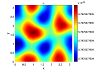
Refer to caption
Refer to caption
Refer to caption
Figure 1: Contour plot of the population densities at t=5000𝑡5000t=5000, when disease transmission rate λ=0𝜆0\lambda=0 and cannibalistic attack rate σ=0.005𝜎0.005\sigma=0.005. Other parameters are fixed as given in (55).
Refer to caption
Figure 2: Bifurcation diagram with bifurcation parameter as disease transmission rate (λ𝜆\lambda). Here 0λ0.020𝜆0.020\leqslant\lambda\leqslant 0.02 and σ=0.005𝜎0.005\sigma=0.005. Other parameters are fixed as given in (55).
Refer to caption
Refer to caption
Refer to caption
Refer to caption
Figure 3: Dynamics of model system (1) at the parameter set, used for the calculation of non-Turing patterns (given in (55)). (a) Three-dimensional phase plot with direction field (b) Two-dimensional phase plot (c) Time series plot and (d) Lyapunov spectrum.
Refer to caption
Refer to caption
Refer to caption
Figure 4: Contour plot of the population densities at t=5000𝑡5000t=5000, when σ=0𝜎0\sigma=0 and λ=0.003𝜆0.003\lambda=0.003. Other parameters are fixed as given in (55).
Refer to caption
Figure 5: Bifurcation diagram with bifurcation parameter as cannibalistic attack rate (σ𝜎\sigma). The range for σ𝜎\sigma is 0σ0.050𝜎0.050\leqslant\sigma\leqslant 0.05 and λ=0.003𝜆0.003\lambda=0.003. Other parameters are fixed as given in (55).
Refer to caption
Refer to caption
Refer to caption
Refer to caption
Figure 6: Dynamics of model system (1) when σ=0.026𝜎0.026\sigma=0.026 and other parameter values are fixed as given in (55). (a) Three-dimensional phase attractor (b) Two-dimensional phase plot (c) Time series plot and (d) Lyapunov spectrum. This is the parameter set at which Turing patterns are seen.
Refer to caption
Refer to caption
Refer to caption
Figure 7: Yellow region shows Turing instability, green region shows planar stablity and brown region shows non-Turing region. Red line represents Hopf bifurcation which separates the Turing and non-Turing regions. Here (a) d2=103,d3=1010formulae-sequencesubscript𝑑2superscript103subscript𝑑3superscript1010d_{2}=10^{-3},d_{3}=10^{-10} (b) d1=105,d3=1010formulae-sequencesubscript𝑑1superscript105subscript𝑑3superscript1010d_{1}=10^{-5},d_{3}=10^{-10} and (c) σ=0.026,d3=1010formulae-sequence𝜎0.026subscript𝑑3superscript1010\sigma=0.026,d_{3}=10^{-10}. Other parameters are same as given in Table 3.
A
Refer to caption Refer to caption Refer to caption
B
Refer to caption Refer to caption Refer to caption
Figure 8: Turing patterns seen in prey, susceptible predator and infected predator densities of model system (3) at (A) t=1000𝑡1000t=1000, the diffusive rate of prey is 105superscript10510^{-5}. (B) t=1000𝑡1000t=1000 and diffusive rate of prey is 106superscript10610^{-6}. Other parameter values are given in Table 3.
A
Refer to caption Refer to caption Refer to caption
B
Refer to caption Refer to caption Refer to caption
C
Refer to caption Refer to caption Refer to caption
D
Refer to caption Refer to caption Refer to caption
Figure 9: Non-stationary non-Turing patterns seen in prey, susceptible predator and infected predator densities of the model system (3), at (A) t=200𝑡200t=200, (B)  t=300𝑡300t=300, (C)  t=500𝑡500t=500, and  (D)  t=1000𝑡1000t=1000. The diffusive constants are d1=106,d2=106formulae-sequencesubscript𝑑1superscript106subscript𝑑2superscript106d_{1}=10^{-6},d_{2}=10^{-6} and d3=1010subscript𝑑3superscript1010d_{3}=10^{-10}. Other parameter values are given in Table 3.
A
Refer to caption Refer to caption Refer to caption
B
Refer to caption Refer to caption Refer to caption
C
Refer to caption Refer to caption Refer to caption
D
Refer to caption Refer to caption Refer to caption
Figure 10: Non-stationary non-Turing patterns seen in prey, susceptible predator and infected predator densities of the model system (3), at (A)  t=1500𝑡1500t=1500,  (B) t=2000𝑡2000t=2000, (C) t=4000𝑡4000t=4000, and  (D)  t=10000.𝑡10000t=10000. The diffusive constants are d1=106,d2=106formulae-sequencesubscript𝑑1superscript106subscript𝑑2superscript106d_{1}=10^{-6},d_{2}=10^{-6} and d3=1010subscript𝑑3superscript1010d_{3}=10^{-10}. Other parameter values are given in Table 3.
A
Refer to caption Refer to caption Refer to caption
B
Refer to caption Refer to caption Refer to caption
C
Refer to caption Refer to caption Refer to caption
D
Refer to caption Refer to caption Refer to caption
Figure 11: Stationary non-Turing patterns seen in prey, susceptible predator and infected predator densities of the model system (3), at (A) t=500𝑡500t=500  (B) t=2000𝑡2000t=2000, (C)  t=3000𝑡3000t=3000, and (D)  t=5000𝑡5000t=5000. The diffusive constants are d1=1010,d2=104formulae-sequencesubscript𝑑1superscript1010subscript𝑑2superscript104d_{1}=10^{-10},d_{2}=10^{-4} and d3=1010subscript𝑑3superscript1010d_{3}=10^{-10}. Other parameter values are given in Table 3.
A
Refer to caption Refer to caption Refer to caption
B
Refer to caption Refer to caption Refer to caption
C
Refer to caption Refer to caption Refer to caption
D
Refer to caption Refer to caption Refer to caption
Figure 12: Stationary non-Turing patterns seen in prey, susceptible predator and infected predator densities of the model system (3), at (A) t=500𝑡500t=500, (B)  t=1000𝑡1000t=1000, (C)  t=1500𝑡1500t=1500, and (D)  t=2000𝑡2000t=2000. The diffusive constants are d1=1010,d2=106formulae-sequencesubscript𝑑1superscript1010subscript𝑑2superscript106d_{1}=10^{-10},d_{2}=10^{-6} and d3=1010subscript𝑑3superscript1010d_{3}=10^{-10}. Other parameter values are given in Table 3.