Guided Random Forest and its application to data approximation

Abstract

We present a new way of constructing an ensemble classifier, named the Guided Random Forest (GRAF) in the sequel. GRAF extends the idea of building oblique decision trees with localized partitioning to obtain a global partitioning. We show that global partitioning bridges the gap between decision trees and boosting algorithms. We empirically demonstrate that global partitioning reduces the generalization error bound. Results on 115 benchmark datasets show that GRAF yields comparable or better results on a majority of datasets. We also present a new way of approximating the datasets in the framework of random forests.

1 Introduction

In supervised learning, one aims to learn a classifier with decision functions that generalize well on unknown samples [1]. In principle, the classifier should have an error rate better than a random guessing on test samples. In ensemble learning, several weak classifiers are trained, and during prediction, their decisions are combined to generate a weighted or unweighted (voting) prediction for test samples. The general idea behind using several weak learners is that their errors are uncorrelated and hence, the probability of all individual classifiers being wrong simultaneously is much lower than their individual error rates.

It has been shown that an ensemble of trees works the best as a general purpose classifier[2]. Amongst several known methods for constructing ensembles, Bagging and Boosting are widely used for tree-based classifiers. For every iteration, bagging generates a new subset of training examples, while boosting assigns higher weights to misclassified samples. The combination of several weak learners eventually results in either axis-aligned decision trees or oblique decision trees. Axis-aligned decision trees[3] recursively split the feature space along directions parallel to the coordinate axes, while oblique decision trees[4, 5, 6, 7, 8, 9] use linear discriminant models, ridge regression[5], principal components of high variance[7, 8] et cetera to obtain the direction of split. However, irrespective of the tree type, for every new split, correction is limited to the region for which the split has been generated.

Here, we propose a classifier termed as Guided Random Forest (GRAF), that extends the outlook of a plane generated for a certain partition, to others as well. GRAF iteratively draws random hyperplanes and further corrects every possible impure partition, such that the overall purity values of resultant partitions increase. The resultant partitions (or leaf nodes) are represented with variable length codes. This process of tree construction eventually bridges the gap between boosting and decision trees, where every tree represents a high variance instance. We also show that GRAF outperforms state of the art bagging and boosting based algorithms like Random Forest[3], Gradient Boosting[10] etc., on several datasets.

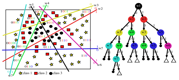
The count of all random hyperplanes generated until a sample falls into its pure partition is used to assign a sensitivity value to the given sample. This assigns higher values of sensitivity to samples that lie in high confusion regions. We also show that sub-sampling of data based on sensitivity scores may well approximate the entire data. Fig. 1 gives an overview of GRAF.

The rest of the paper is organized as follows: Section #2 gives details about GRAF; Section #3 explains the relationship of GRAF with boosting; Section #4 gives the implementation details of the algorithm; Section #5 studies trends in bias-variance and strength-correlation from the perspective of GRAF; approximation of data using their sensitivity scores is studied in Section #6; Section #7 contains concluding remarks.

Figure 1: An overview of the creation of high variance instances in GRAF. Every instance consists of sub-spacing the dataset in a uniformly sampled feature space. A random hyperplane is generated for the sub-spaced samples. It assigns bit 0/1 to every sample. A pure (impure) partition is a partition containing all (some) samples of the same class. Amongst these partitions, the most impure partition affects the generation of the next hyperplane. This hyperplane is extended to the other partition as well if it improves the purity of subsequent partitions in that region. This generation of hyperplanes is continued until all partitions are maximally purified. At an intermediate stage, partitions are either pure or impure. To increase the confidence of classification, the above process is repeated to create $L$ high variance instances.

2 Guided Random Forest (GRAF)

Let, $\mathscr{X}\in\mathbb{R}^{d}$ denote the input space and $\mathscr{Y}$ denote a set of $C$ classes $\{1,...,C\}$. Let a set $S$ contains $N$ samples drawn i.i.d. according to some distribution $\mathscr{D}$ over $\mathscr{X}\times\mathscr{Y}$.

Let us assume $\mathscr{T}$ high variance classifier instances are constructed on the dataset $S$. For every instance $k\in\{1,...,\mathscr{T}\}$, consider $h_{k}\in H$, such that $h_{k}:\mathscr{X}\times\mathscr{Y}\to\mathbb{R}$. Also, assume a set $\Lambda$ such that $\lambda\in\Lambda$ and $\lambda:\mathscr{X}\to\{0,1\}$, and $f:\{0,1\}^{r}\times\mathscr{Y}\to\mathbb{R}$, $r\in\mathbb{N}$.

The training of an instance involves the addition of random hyperplanes in a forward stagewise fashion. At a given step, the combination of these hyperplanes divides the space into $T_{p}$ partitions. Every partition $\Omega_{p}$ consists of a set of samples $A_{\Omega_{p}}$, with the same code (composed of 0s and 1s). A partition is said to be pure if it contains samples of the same class or samples from different classes cannot be separated further. On the other hand, a partition is said to be impure if it contains samples of different classes, that can be further dichotomized by the addition of new hyperplanes (Fig. 1). Let us assume a set $\hat{\Omega}$ of partitions $\Omega_{p}$, such that

$$\hat{\Omega}=\bigcup_{p=1}^{p=T_{p}}\{\Omega_{p}\}$$ (1)

$$\Omega_{p}=\left(\lambda^{\Omega_{p}},A_{\Omega_{p}}\right)\text{; where}\\ \begin{cases}A_{\Omega_{p}}\subseteq S\\ |\Omega_{p}|=|A_{\Omega_{p}}|=n_{\Omega_{p}}\\ (x^{i},y_{i})\in A_{\Omega_{p}}\Leftrightarrow(x^{i},y_{i})\in\Omega_{p},\>\forall(x^{i},y_{i})\in A_{\Omega_{p}}\\ \Omega_{i}\cap\Omega_{j}=A_{\Omega_{i}}\cap A_{\Omega_{j}}=\emptyset,\>\forall i,j\in{1,...,T_{p}}\land i\neq j\end{cases}$$ (2)

For a given sample $(x^{i},y_{i})\in\Omega_{p}$, $\lambda^{\Omega_{p}}$ generates bit 0 or 1, such that $W^{\Omega_{p}}=[w_{1}^{\Omega_{p}},...,w_{d}^{\Omega_{p}}]$ dichotomizes the partition $\Omega_{p}$.

$$\lambda^{\Omega_{p}}(x^{i})=\mathbbm{1}{\left(\sum_{j=1}^{d}(w_{j}^{\Omega_{p}}x^{i}_{j})+bias^{\Omega_{p}}>0\right)},\\ \lambda^{\Omega_{p}}\in\Lambda,(x^{i},y_{i})\in A_{\Omega_{p}}$$ (3)

where $\mathbbm{1}(.)$ is the indicator function.

$$w_{j}^{\Omega_{p}}\sim U(min_{j}^{\Omega_{p}}+\varepsilon,max_{j}^{\Omega_{p}}-\varepsilon),\\ \forall j\in\{1,...,d\},\>\varepsilon\approx 0,\varepsilon>0$$ (4)

where $U(a,b)$ is uniform distribution.

$$bias^{\Omega_{p}}=-\sum_{j=1}^{d}w_{j}^{\Omega_{p}}\mu_{j}^{\Omega_{p}}$$ (5)

$$min_{j}^{\Omega_{p}}=\min_{i\in\{1,...,n_{\Omega_{p}}\}}x^{i}_{j}\text{, }(x^{i},y_{i})\in A_{\Omega_{p}},\>j\in\{1,..,d\}$$ (6)

$$max_{j}^{\Omega_{p}}=\max_{i\in\{1,...,n_{\Omega_{p}}\}}x^{i}_{j},\>(x^{i},y_{i})\in A_{\Omega_{p}},\>j\in\{1,..,d\}$$ (7)

$$\mu_{j}^{\Omega_{p}}=\frac{1}{n_{\Omega_{p}}}\sum_{i=1}^{n_{\Omega_{p}}}x^{i}_{j},\>(x^{i},y_{i})\in A_{\Omega_{p}},\>j\in\{1,..,d\}$$ (8)

If $|\Omega_{p}|=0$, then it is termed as an empty partition. Hence, we define a set $\Omega$ that consists of only non-empty partitions.

$$\Omega=\{\Omega_{i}:|\Omega_{i}|>0,\>\forall i\in\{1,...,|\hat{\Omega}|\}\}$$ (9)

The process of hyperplane generation follows a greedy approach. We choose the most impure partition in an attempt to purify it.

We define a function $Z:\Omega\to\mathbb{R}$, which yields the impurity content of a partition, such that if $\Omega_{p}=\Omega_{p0}\cup\Omega_{p1}$, then $Z(\Omega_{p})\geq Z(\Omega_{p0})+Z(\Omega_{p1})$.

We have used the following impurity function.

$$Z(\Omega_{p})=\left(1-\sum_{c=1}^{C}(\frac{|\Omega_{p}|_{c}}{N_{c}})^{2}\times(\sum_{c=1}^{C}\frac{|\Omega_{p}|_{c}}{N_{c}})^{-2}\right)\times|\Omega_{p}|$$ (10)

where $N_{c}$ denotes the total samples of class $c$, and $|\Omega_{p}|_{c}$ denotes the samples of class $c$ in partition $\Omega_{p}$.

Further, we define $\Omega^{{}^{\prime}}\subseteq\Omega$, which consists of only impure partitions, that can be further divided

$$\Omega^{{}^{\prime}}=\{\Omega_{i}:(Z(\Omega_{i})>0)\land((min_{j}^{\Omega_{i}}\neq max_{j}^{\Omega_{i}})\\ \exists j\in\{1,..,d\})\>\forall i\in\{1,...,|\Omega|\}\}$$ (11)

Given $\Omega^{{}^{\prime}}$, the most impure partition $\omega$ is considered

$$\omega=\arg\max_{\Omega_{i}\in\Omega^{{}^{\prime}}}Z(\Omega_{i})$$ (12)

Divide partition $\omega$, such that

$$\begin{cases}\omega_{0}=\{(x^{i},y_{i}):\lambda^{\omega}(x^{i})=0\>\forall(x^{i},y_{i})\in A_{\omega}\}\\ \omega_{1}=\{(x^{i},y_{i}):\lambda^{\omega}(x^{i})=1\>\forall(x^{i},y_{i})\in A_{\omega}\}\end{cases}$$ (13)

The effect of this hyperplane is extended to other impure partitions as well. In effect, the given space of samples is divided into maximal pure partitions.

For the remaining partitions, $\phi\in\Omega^{{}^{\prime}}\setminus\{\omega\}$, we extend the effect of $W^{\omega}$ to them as well.

$$\begin{cases}\phi_{0}=\{(x^{i},y_{i}):\lambda^{\omega}(x^{i})=0\>\forall(x^{i},y_{i})\in A_{\phi}\}\\ \phi_{1}=\{(x^{i},y_{i}):\lambda^{\omega}(x^{i})=1\>\forall(x^{i},y_{i})\in A_{\phi}\}\end{cases}$$ (14)

Now, update the set of impure partitions $\Omega^{{}^{\prime}}$, such that it consists of only new partitions, that are impure and non-empty.

$$\Omega^{{}^{\prime}}=\bigcup_{\begin{subarray}{c}(\phi\in\Omega^{{}^{\prime}})\\ \land(i\in\{0,1\})\end{subarray}}\{(\lambda^{\omega},A_{\phi_{i}}):|A_{\phi_{i}}|>1\>\land\>Z(\lambda^{\omega},A_{\phi_{i}})>0\}$$ (15)

The above process is repeated till there is no more impure partition left to be further dichotomized, i.e., $|\Omega^{{}^{\prime}}|=0$.

Once the above process is completed, we collect all pure partitions in a set $\tilde{\Omega}$.

$$\tilde{\Omega}=\{\Omega_{i}:(|\Omega_{i}|>0)\land((Z(\Omega_{i})=0)\lor((min_{j}^{\Omega_{i}}=max_{j}^{\Omega_{i}})\\ \forall j\in\{1,..,d\}))\>\forall i\in\{i,..,|\hat{\Omega}|\}\}$$ (16)

For every pure partition, a code is assigned and it is shared by every sample in the partition. Assuming that all the partitions have been placed in an arbitrary order $\bar{\Omega}=(\tilde{\Omega})$, then

$$code_{x^{i}}=(\lambda^{\Omega_{p}}(x^{i}):\forall\Omega_{p}\in\bar{\Omega})\text{ }\forall(x^{i},y_{i})\in S$$ (17)

The proportion of samples from different classes in resultant partitions represents their probability. For a given test sample, these probabilities are combined across all instances, and the class with the highest probability is associated with it.

$f$ maps every pure partition (represented by its unique code) to the posterior probabilities of finding a class $c\in\mathscr{Y}$ in the given partition.

$$\hat{f}{(code_{x^{i}},y_{i})}=\\ \frac{|\{y_{j}:(y_{j}=y_{i})\land(code_{x^{j}}=code_{x^{i}})\}\>\forall j\in\{1,..,S\}|}{|\{y_{j}:code_{x^{j}}=code_{x^{i}}\}\>\forall j\in\{1,..,S\}|}$$ (18)

Let, $IF_{c}$ denote the weight associated with a class $c$ such that abundant classes have lesser weights and vice-versa.

$$IF_{c}=\frac{|S|}{|\{y_{j}:y_{j}=c\}\>\forall j\in\{1,..,S\}|}\>\forall c\in\{1,...,C\}$$ (19)

To handle class imbalance,

$$f{(code_{x^{i}},y_{i})}=\frac{\hat{f}{(code_{x^{i}},y_{i})}\times IF_{y_{i}}}{\sum_{c=1}^{C}IF_{c}\times\hat{f}{(code_{x^{i}},c)}}$$ (20)

Further, we define $h_{k}$ as follows which maps every pure partition to its posterior probabilities.

$$h_{k}(x^{i},y_{i})=f(code_{x^{i}},y_{i})\>\forall(x^{i},y_{i})\in\mathscr{X}\times\mathscr{Y}$$ (21)

The above steps represent the construction of one high variance classifier instance. However, it is well established in the literature that an ensemble of such high variance instances, in general, tends to yield better generalization on test samples[11]. GRAF creates several such high variance instances. Further, to minimize the correlation between these classifiers, GRAF employs random sub-spacing.

Next, we define $H_{t}$ such that it maps a sample to a class by using a consensus for prediction that be reached by computing the joint probability of predictions returned by each high variance classifier.

$$H_{t}:\mathscr{X}\to\mathscr{Y}$$ (22)

$$H_{t}(x^{i})=\arg\max_{y_{i}\in\mathscr{Y}}\sum_{k=1}^{\mathscr{T}}\log_{2}\left(1+h_{k}(x^{i},y_{i})\right)$$ (23)

It should be noted that when all partitions for sample $x^{i}$ contain only one class $c$, then $h_{k}(x^{i},c)$ is 1 for $c$ and 0 for remaining classes. Hence, $H_{t}(x^{i})$ is equivalent to a voting classifier.

Given an ensemble of instances $h_{1}$, $h_{2}$,…,$h_{\mathscr{T}}$, GRAF optimizes the margin function as follows

$$mg(x^{i},y_{i})=\mathbbm{1}{\left(H_{t}(x^{i})=y_{i}\right)}-\max_{y_{j}\in Y\setminus{y_{i}}}\mathbbm{1}{\left(H_{t}(x^{i})=y_{j}\right)}$$ (24)

Hence, the margin over the complete set of samples $\mathscr{X}\times\mathscr{Y}$ is defined as

$$mg=\mathbb{E}_{\mathscr{X},\mathscr{Y}}mg(x^{i},y_{i})$$ (25)

3 Relationship of GRAF with boosting

As shown in Algorithm 1, the construction of a high variance instance of a classifier can be abstracted as a boosting algorithm[12]. Assuming the weight of each sample to be $1$ initially, a random hyperplane is generated (equation 3). This generated hyperplane divides the region into two parts. Sample weights are updated to focus on the part under consideration, based on their impurity (equation 10). All the samples in that part are assigned weight $1$ while remaining samples are assigned weight $0$. A new random hyperplane is generated (equation 4) based on the weight distribution of samples. However, this new plane is extended to other partitions as well. The combination of all these planes (hypotheses) increases the confidence and hence, eventually creates a strong learner.

Algorithm 1 High variance instance of GRAF as boosting

Input:$(x^{1},y_{1})$,…,$(x^{N},y_{N})$; $x^{i}\in\mathscr{X}$, $y_{i}\in\{1,...,C\}$, $C$ denotes the total unique classes and $N$ denotes the total training samples.

         $Z:\Omega\to\mathbb{R}$ where $\Omega$ constitutes a set of points with same code.

         $\mathscr{Y}=\{1,...,C\}$

Initialize: $P(i)\leftarrow 1\>\forall i\in\{1,...,N\}$

             $\textit{code}(i)\leftarrow\varnothing\>\forall i\in\{1,...,N\}$

until $\sum_{i=1}^{i=N}P(i)=0$ do

       Choose a random hypothesis using $P(i)$, such that $\lambda:\mathscr{X}\to\{0,1\}$

       $\textit{code}(i)\leftarrow\textit{code}(i)\cup\{\lambda(x^{i})\}\>\forall i\in\{1,...,N\}$

       Let $\Omega{{}_{i}}\leftarrow\{(x^{j},y_{j}):code(j)=code(i)\>\forall j\in\{1,...,N\}\}\>\forall i\in\{1,...,N\}$

       $\omega\leftarrow\arg\max_{i\in\{1,...,N\}}Z(\Omega_{i})$

       Update $P(i)\leftarrow\mathbbm{1}{\left(\Omega_{i}=\Omega_{\omega}\right)}\>\forall i\in\{1,...,N\}$

4 Implementation details

Guided random forest (GRAF) creates an ensemble classifier, by repeatedly partitioning the space into two parts. To build an instance of a classifier from a given set $S$ of samples, a subset of $M$ features is uniformly sampled from the given set of features $d$. The given samples are then projected into M-dimensional sub-spaces, denoted by $\mathscr{X}_{M}$. To facilitate efficient implementation, the additive construction of an instance is represented as a tree from the beginning. The tree is represented by its collection of nodes and partitions (Algorithm A1 and Fig. 2). At $0$-th height, $root\_node$ and $root\_partition$ consist of all samples, $(x^{{}^{\prime}})^{i}\in\mathscr{X}_{M}$ and hence, the weight vector $W^{\textit{height}}$ is weighted by all samples. At every height, the most impure partition $\omega$ (Algorithm A4), affects the generation of $W^{\textit{height}}$ and $bias^{\textit{height}}$. Thus, $W^{\textit{height}}$ and $bias^{\textit{height}}$ represent the weight vector $W^{\omega}$, and $bias^{\omega}$, respectively (equations 3 - 8). At a given height there exists a set of empty, pure and impure partitions. The total number of these partitions are $\sum_{i=0}^{M}\binom{height}{i}$ (for $height<i$, $\binom{height}{i}=0$), i.e., it is a polynomial in $height$ of the order of $M$ ($\mathcal{O}(height^{M})$). Thus, the number of filled (pure and impure) partitions is $\mathcal{O}(\min(|S|,\sum_{i=0}^{M}\binom{height}{i}))$. For further processing, only impure partitions need to be considered. Hence, a set $\Omega^{{}^{\prime}}$ consists of only impure partitions. The most impure partition $\omega\in\Omega^{{}^{\prime}}$ defines the distribution of the next random weight vector (hyperplane or $W^{\omega}$) to be included at next height. The effect of the hyperplane is extended to other impure partitions as well. Even though $W^{\omega}$ almost surely dichotomizes the partition $\omega$, it may or may not dichotomize other remaining partitions in the set $\Omega^{{}^{\prime}}$. To avoid empty partitions from being created, the bit assignment is skipped for the non-dichotomized partition at a given height ($b^{\textit{height}}$). Hence, the resultant $code(j)$ for sample $x^{j}$ in partition $\Omega_{j}$, formed by the concatenation of $b^{\textit{height}}_{j}$, is of variable length. Once all impure partitions have been fixed, leaf nodes represent the posterior probabilities of a class (Algorithm A3). The above procedure is repeated for the construction of other trees, with a different random sub-space of features of length $M$. Algorithms A2 and A5 highlight the training and testing procedures of GRAF.

Figure 2: Partitioning of space in GRAF is represented by a tree. A partition, containing a subset of samples, is defined by its unique combination of hyperplanes. However, these hyperplanes may affect the formation of other partitions. Once the space is maximally partitioned such that impurity in any partition cannot be reduced further, the process terminates. Every resultant partition is a leaf node in the tree, represented by a dot in figure. (A triangle denotes an impure partition which may be dichotomized further.)

5 Results

5.1 Bias-variance tradeoff

In order to understand the behavior of a classifier, it is imperative to study its bias-variance tradeoff. A classifier with a low bias has a higher probability of predicting the correct class than any other class, i.e., the predicted output is much closer to the true output. On the other hand, the classifier with low variance indicates that its performance does not deviate for a given test set across several different models. There are several methods to evaluate bias-variance tradeoff for 0-1 loss on classification learning[13, 14, 15, 16]. Of these, we use the definitions of Kohavi & Wolpert[14] for bias-variance decomposition.

For the analysis of bias-variance tradeoff, $N/2$ samples were set aside as the test set. From the remaining dataset, $R$ overlapping training sets of the same size $N_{m}$ were created, and $R$ models were trained. For every model, the estimate $\hat{y_{i}}$ is obtained for every instance $i$ in the test set, whose size is denoted by $N_{t}$.

$$p^{i}_{j}=\frac{1}{R}\sum_{r=1}^{r=R}\mathbbm{1}{(\hat{y_{i}}=j})$$ (26)

$$bias^{2}=\frac{1}{N_{t}}\Bigg{(}\sum_{i=1}^{i=N_{t}}\sum_{j=1}^{j=C}\big{(}(\mathbbm{1}{(y_{i}=j)}-p^{i}_{j})^{2}-\frac{p^{i}_{j}*(1-p^{i}_{j})}{R-1}\big{)}\Bigg{)}$$ (27)

$$variance=1-\frac{1}{N_{t}}\sum_{i=1}^{i=N_{t}}\sum_{j=1}^{j=C}(p^{i}_{j})^{2}$$ (28)

$$err=\frac{1}{R}\sum_{r=1}^{r=R}\Big{(}1-\frac{1}{N_{t}}\sum_{i=1}^{i=N_{t}}\mathbbm{1}{(y_{i}=\hat{y_{i}})}\Big{)}$$ (29)

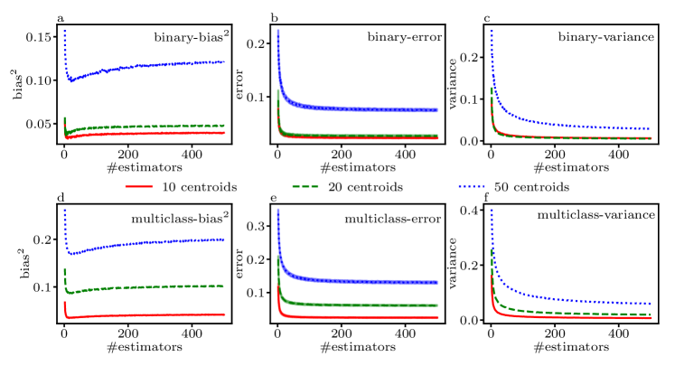
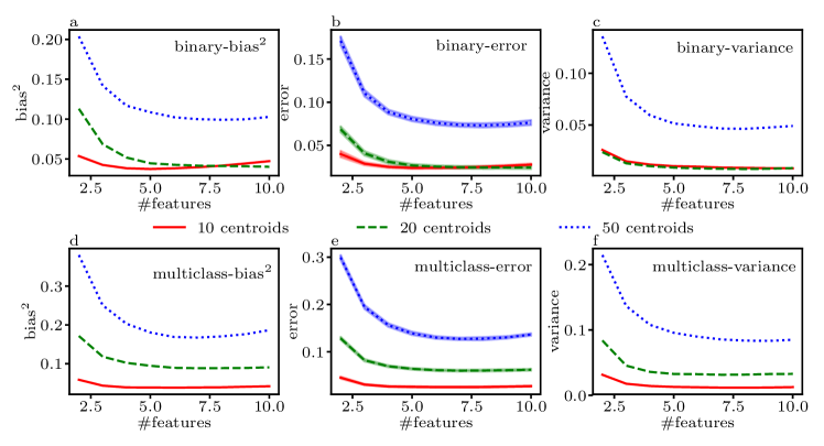
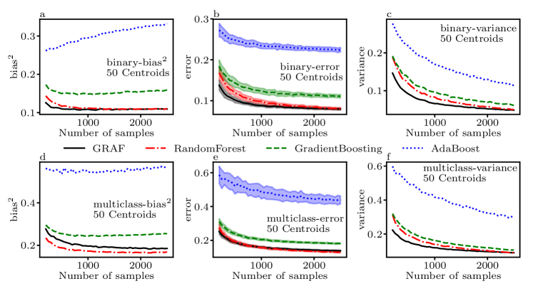
Two different studies were performed to evaluate the performance of GRAF in terms of bias and variance decomposition. First, the effect of different values of hyper-parameters (namely, number of trees and feature sub-space size) on the bias, variance, and the misclassification error rate was analyzed. Second, the trends of bias and variance were observed for increasing train set sizes and compared with different classifiers. To perform these analyses, 6 different binary and multi-class datasets with different values of centres were chosen from {10, 20, 50}, and were simulated by using Weka[17]. Each dataset consisted of 10000 samples and 10 features (generated using RandomRBF class), while other parameters were set as default. To create the test set, $5000$ samples were randomly selected. For a given train dataset size ($200\leq N_{m}\leq 2500$), 50 models were generated by repeatedly sampling without replacement, from the remaining dataset.

The effect of increasing the number of trees from 2 to 500 is illustrated in Fig. 3. For intermediate values of the numbers of trees, bias-variance curves saturate to their minima, and hence, the average misclassification converges to its minimum. It implies that higher accuracies can be achieved well before all trees are used[18]. Fig. 4 highlights the effect of increasing the number of randomly selected dimensions/features. This figure shows that a subset of features, in general, may be enough to generate the desired results. However, the selected sub-space must be large enough to distinguish the samples in this sub-space. For these experiments $N_{m}$ was set to $2500$.

In a different study, the influence of an increasing number of training samples ($200\leq N_{m}\leq 2500$) is illustrated in Fig. 5 for a dataset with 50 centroids (Figures A1 & A2 are for 10 and 20 centroids, respectively). Bias and variance decrease with an increase in the size of the training set. In general, GRAF was found to have the least variance, and the lowest or comparable misclassification errors on test samples, when compared with other methods (default values of hyper-parameters are used, $L=100$ and $M=5$).

Figure 3: Bias-variance analysis with an increasing number of estimators (trees) in a classifier. For both binary (a-c) and multi-class (d-f) datasets with different values of centroids (10, 20, and 50), the number of estimators is increased from $2$ to $500$, while fixing the number of dimensions to be sampled $(M=d/2)$. As the number of estimators is increased, bias, error, and variance rapidly saturate.

Figure 4: Bias-variance analysis with an increasing number of dimensions (features) selected from a given feature space in a classifier. For both binary (a-c) and multi-class (d-f) datasets with different values of centroids (10, 20, and 50), $M$ is increased from $2$ to $10$, while fixing the number of estimators to be assembled $(L=100)$. When the dimension of the sub-space is large enough to distinguish samples of different classes, bias and variance saturate and converge to their minimum. With increasing dimensionality of the sub-space, misclassification error continues to decrease and rapidly saturates to its minimum.

Figure 5: Bias-variance analysis with an increasing samples in a training set. For both binary (a-c) and multi-class (d-f) datasets with 50 centroids, the number of samples is increased from $200$ to $2500$, while fixing the number of dimensions to be sampled $(M=d/2)$ and the number of estimators as $L=100$. As the cardinality of the training set is increased, bias-variance continues to decrease, and the misclassification error continues to decrease and may saturate to its minimum.

5.2 Study of strength and correlation

For an ensemble of trees, an upper bound on the generalization error ($PE^{*}$) is determined using two parameters, i.e., strength ($s$) and correlation ($\rho$)[19, 3]. For optimum generalization error, both parameters are important. Strength measures the confidence of every instance (tree) of a classifier in predicting the true label of every instance in a test set, while correlation measures the dependence between these instances.

$$PE^{*}\leq\bar{\rho}(1-s^{2})/s^{2}$$ (30)

where $\bar{\rho}$ is the mean of the correlation.

$$p_{i}=\frac{1}{\mathscr{T}}\sum_{t=1}^{t=\mathscr{T}}\mathbbm{1}{(\hat{y}_{i}^{t}=y_{i})}-\max_{\begin{subarray}{c}j\in\{1,...,C\}\\ \land j\neq y_{i}\end{subarray}}\frac{1}{\mathscr{T}}\sum_{t=1}^{t=\mathscr{T}}\mathbbm{1}{(\hat{y}_{i}^{t}=j)}\\ \forall i\in\{1,...,N_{t}\}$$ (31)

where $\hat{y}_{i}^{t}$ denotes the prediction of instance $i$ by tree $t$.

$$acc_{t}=\frac{1}{N_{t}}\sum_{i=1}^{i=N_{t}}\mathbbm{1}{(\hat{y}_{i}^{t}=y_{i})}\>\>\>\forall t\in\{1,...,\mathscr{T}\}$$ (32)

$$sec_{t}=\frac{1}{N_{t}}\sum_{i=1}^{i=N_{t}}\mathbbm{1}{(\hat{y}_{i}^{t}=\arg\max_{\begin{subarray}{c}j\in\{1,...,C\}\\ \land j\neq y_{i}\end{subarray}}\frac{1}{\mathscr{T}}\big{(}\sum_{k=1}^{k=\mathscr{T}}\mathbbm{1}{(\hat{y}_{i}^{k}=j)}\big{)})}\\ \forall t\in\{1,...,\mathscr{T}\}$$ (33)

$$sd=\frac{1}{\mathscr{T}}\sum_{t=1}^{t=\mathscr{T}}\sqrt{acc_{t}+sec_{t}-acc_{t}^{2}-sec_{t}^{2}}$$ (34)

$$s=\frac{1}{N_{t}}\sum_{i=1}^{i=N_{t}}p_{i}$$ (35)

$$\rho=\frac{1}{sd^{2}}\left(\frac{1}{N_{t}}\sum_{i=1}^{i=N_{t}}p_{i}^{2}-s^{2}\right)$$ (36)

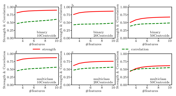
For analysis, binary and multi-class datasets were generated using Weka[17], as discussed in section 5.1. The number of dimensions selected from a given feature space was varied from $3$ to $10$. For a given dimensionality of the sub-space, $80$ models were generated by randomly sampling $9000$ samples for training, while $1000$ samples were kept aside for testing the generated model. Further, strength and correlation were computed using equations 35 and 36, respectively.

Fig. 6 shows the effect of increasing dimensions on various instances of binary and multi-class datasets. Notably, as the number of features is increased, strength increases and eventually saturates, while correlation continues to increase.

Figure 6: Strength and correlation analysis with increasing number of features (dimensions) selected from a given feature space in a classifier. For both binary (a-c) and multi-class (d-f) datasets with different values of centroids (10, 20, and 50), $M$ is increased from $3$ to $10$, while fixing the number of estimators to be assembled $(L=100)$. With increasing dimensionality of the sub-space, strength saturates, and correlation continues to increase.

5.3 Performance comparison on UCI datasets

The performance of GRAF has been evaluated on 115 UCI datasets[20] and compared against random forest[3], gradient boosting[10], and adaboost[12]. For comparison, we used the strategy as defined in Fernandez-Delgado et al.[2]. It uses 4-fold cross-validation on the whole dataset to compute the accuracy. The training dataset contains 50% of the total samples. The hyper-parameters are tuned using 5-fold cross-validation on the training dataset.

For all methods, the number of estimators is tuned from $\{100,200,500,1000,2000\}$. For GRAF, random forest, and gradient boosting, the number of dimensions to be selected has been tuned from $\{\log_{2}(d),\sqrt{d},d/2,d\}$, and the node is further split only if it has minimum samples, tuned between 2 and 5.

The average of the test set accuracies across 4-folds of cross-validation has been tabulated in Table A1. For every dataset, the method with the highest accuracy has been highlighted. On 53 datasets, GRAF either outperforms or performs as good as other methods. On 94, 69, and 67 datasets, the performance of GRAF is either better or comparable, when compared with only adaboost, random forest, and gradient boosting, respectively. The other interesting observation is that GRAF has comparable or improved accuracies on UCI datasets of plant-margin, plant-shape, and plant-texture, which consist of the highest number of classes (100), when compared with other datasets considered for comparison.

6 Sensitivity

We define the sensitivity of a partition as the number of weights required to create it. It follows from the idea that regions with higher confusion will require more weights to create pure partitions. We define a region with confusion as one in which samples of many different classes reside. We argue that points in these regions are crucial for the approximation of data, as these points have a major influence in defining the decision region.

We also define the sensitivity of a point as a function of the number of weights required to put that sample into a pure partition. To assign a sensitivity value to every point in a partition, first, we rank each point in the partition arbitrarily and divide the sensitivity associated with a partition by point’s rank. Second, we normalize these values class-wise. If the partition is big, ranked sensitivity prevents sensitivity scores from being overwhelmed with the points from a single partition. On the other hand, class-wise normalization handles an imbalance in the data by assigning higher sensitivities to less populated classes. Formally, we represent the process as follows.

Let us assume, $\mathscr{W}:\Omega\to\mathbb{N}$ maps each partition to the number of weights required to pure it. Hence, the importance of each sample $x^{i}$ in partition $\omega\in\Omega$ can be computed as

$$\theta_{\omega x^{i}}=\frac{\mathscr{W(\omega)}}{i}\>\>\forall i\in\{1,...,|\omega|\}\>\>\forall\omega\in\Omega$$ (37)

Equation 37 assigns each sample in dataset an importance value, based on the size of partition $\omega$. Assume that the importance of a sample in dataset is given by $\theta_{x^{i}}$ $\forall i\in\{1,...,N\}$. Assuming that $X_{j}=\{x^{k}:y_{k}=j\>\>\forall k\in\{1,...,N\}\}$ $\forall j\in\{1,...,C\}$ represents a set of samples belonging to a class, the sensitivity of each sample can be computed as

$$s_{i}=\ln\left(1+\frac{\theta_{x^{i}}}{\Theta_{y_{i}}}\right)\>\>\forall i\in\{1,...,N\},\text{ where }\\ \Theta_{j}=\sum_{x^{k}\in X_{j}}\theta_{x^{k}},\>\>\forall j\in\{1,...,C\}$$ (38)

Assuming that each sample is assigned a sensitivity $s_{i}^{t}$ $\forall t\in\{1,...,\mathscr{T}\}\land\forall i\in\{1,...,N\}$, the mean sensitivity of each sample can be defined as

$$\hat{s}_{i}=\frac{1}{\mathscr{T}}\sum_{t=1}^{t=\mathscr{T}}s_{i}^{t}$$ (39)

Hence, the probability of each sample can be defined as

$$p_{i}=\frac{\hat{s}_{i}}{\sum_{j=1}^{j=N}\hat{s}_{j}},\>\forall i\in\{1,...,N\}$$ (40)

The higher the probability or sensitivity of a sample, the more important it is.

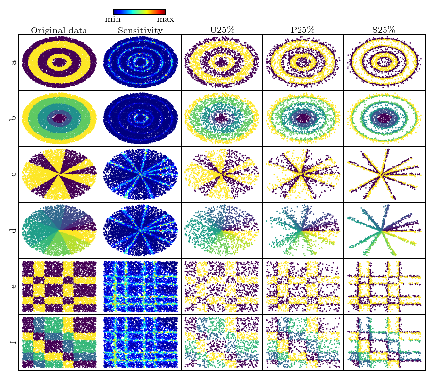
The sensitivities associated with the samples may be used to approximate the complete dataset, for further downstream analyses with high sensitivity points only. A study was designed to assess how well the sensitivity computed using GRAF approximates different datasets. To perform this analysis, 6 different datasets were created. Every dataset consists of samples distributed in different patterns (concentric circles, pie-charts, and XOR representations). For every pattern, both binary and multi-class versions were generated as illustrated in Fig. 7. To generate sensitivity scores on each dataset, 200 trees ($L=200$) with complete features space ($M=2$) were generated and sensitivity score ($\hat{s}_{i}$) was computed. The performance of GRAFś sensitivity has been compared with a uniform distribution for samples. Fig. 7 illustrates that when only 25% of the total points are sampled, samples with the highest sensitivities adequately approximate the regions with the highest confusion.

Figure 7: Assessment of performance of GRAFś sensitivity on simulated binary and multi-class datasets. (a, c, and e) represent simulated datasets with binary classes. (b, d, and f) represent simulated multi-class datasets. The classes are arranged in different patterns, concentric circles, pie-charts, and XOR representations, in a-b, c-d, and e-f, respectively. For each of these datasets, the distribution of sensitivities computed using GRAF has been shown in column Sensitivity. A point with higher sensitivity indicates that it is more important for data approximation. The other columns U25%, P25%, and S25%, compare the performances of data approximation using only 25% of the total samples, sampled using a uniform distribution, distribution defined by GRAFś sensitivity, and the points with the highest values of sensitivities, respectively. The regions with the most confusion are best approximated using points with the highest sensitivities.

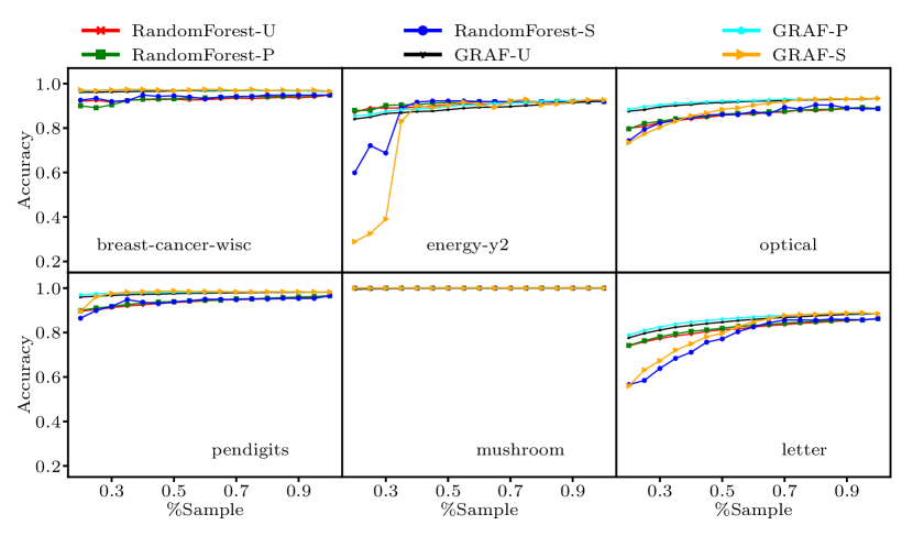
The other study on some of the UCI datasets[20] also conforms to the fact that points sampled using distribution defined by their sensitivities perform comparable or better when compared with points sampled using uniform distribution. Also, for a given dataset, the maximal accuracy on a test set can be achieved by using only a fraction of its samples with the highest sensitivities (Fig. 8). Similar trends in results are observed, irrespective of the method (Random forest[3] or GRAF) used for learning the model. To perform this experiment, 200 trees ($L=200$) were generated, and the number of features ($M$) was chosen as per the tuned model, and sensitivity scores were computed on the resulting trees.

Figure 8: Performance evaluation of Random forest[3] and GRAF, with increasing fraction of samples used for training, sampled according to uniform distribution (U), their sensitivities (P), and their decreasing order of sensitivities (S). The points sampled using distribution defined by their sensitivities perform comparable or better when compared with points sampled using uniform distribution. Also, as points are added in the decreasing order of their sensitivities, the accuracy on test set converges and reaches its maximum with only a fraction of points with high sensitivities. The trends in results are similar, irrespective of the method used for classification.

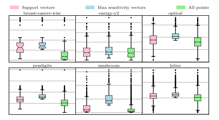
The extension of the previous study has been done to show that high sensitivity points are analogous to support vectors. Table I records the accuracies on a given test set when a SVM model was trained using all the samples in the training set. These results were compared with a SVM model that is trained using only high sensitivity points. The number of such points was chosen so that it constituted the same fraction as that of support vectors. An analogy between support vectors and the fraction of points with high sensitivity has also been illustrated in Fig. 9.

	#Train Samples	%Support Vectors	%Overlap of high sensitivity points with support vectors	%SVM accuracy	%SVM accuracy on high sensitivity points
synthetic-control	300	55.667	66.467	99.00	98.00
credit-approval	345	53.623	74.595	87.54	87.54
breast-cancer-wisc	350	17.429	60.656	96.85	96.85
energy-y2	384	80.729	84.839	90.89	90.89
statlog-vehicle	423	52.719	58.296	79.91	79.91
statlog-german-credit	500	60.800	84.211	74.00	74.20
optical	1912	39.331	49.468	98.33	95.86
pendigits	3747	19.509	44.870	99.52	98.05
mushroom	4062	11.177	25.110	100	100
letter	10000	52.190	65.644	96.53	92.34

TABLE I: Equivalence between high sensitivity points and support vectors. For a given test set, the SVM model is learned using two different sets. First, a SVM model is trained using all the samples in the training set. Then its accuracy on the test set is evaluated (column % SVM accuracy), and information about the support vectors is recorded (column % Support vectors). Separately, a SVM model is trained using the points with high sensitivity with their fraction chosen to be the same as that of support vectors (column % SVM accuracy on high sensitivity points). An analogy between points with high sensitivity and support vectors is recorded in column % Overlap of high sensitivity points with support vectors.

Figure 9: An analogy between support vectors and points with high sensitivities. The distribution of probabilities (equation 40) associated with support vectors has been compared with that of a fraction of points with high sensitivities, and the distribution of probabilities associated with all points. It can be concluded that points with higher sensitivities coincide with the support vectors with higher values of weights.

7 Conclusion

In this paper, we discuss a guided approach to constructing random forests, termed as Guided Random Forest (GRAF). GRAF repeatedly draws random hyperplanes to partition the data. It uses successive hyperplanes to correct impure partitions to the extent feasible, so that the overall purity of resultant partitions increases. The resultant partitions (or leaf nodes) are represented with variable length codes. This guided tree construction bridges the gap between boosting and decision trees, where every tree represents a high variance instance. Results on 115 benchmark datasets show that GRAF outperforms state of the art bagging and boosting based algorithms like Random Forest[3] and Gradient Boosting[10]. The results show that GRAF is effective on both binary and multi-class datasets. It provides both low bias and low variance with increasing size of the training dataset. We introduce the notion of sensitivity, a metric that indicates the importance of a sample. We illustrate that GRAF can be used to approximate a given dataset by using only a few points with high sensitivity. The proposed sensitivity scheme does not dwell into selection criteria for a subset of points. However, it differentiates between points on the basis of their proximity to confusion regions, akin to support vectors in kernel schemes.

References

- [1] T. G. Dietterich, “Ensemble methods in machine learning,” in International workshop on multiple classifier systems. Springer, 2000, pp. 1–15.
- [2] M. Fernández-Delgado, E. Cernadas, S. Barro, and D. Amorim, “Do we need hundreds of classifiers to solve real world classification problems?” The Journal of Machine Learning Research, vol. 15, no. 1, pp. 3133–3181, 2014.
- [3] L. Breiman, “Random forests,” Machine learning, vol. 45, no. 1, pp. 5–32, 2001.
- [4] R. Blaser and P. Fryzlewicz, “Random rotation ensembles,” The Journal of Machine Learning Research, vol. 17, no. 1, pp. 126–151, 2016.
- [5] B. H. Menze, B. M. Kelm, D. N. Splitthoff, U. Koethe, and F. A. Hamprecht, “On oblique random forests,” in Joint European Conference on Machine Learning and Knowledge Discovery in Databases. Springer, 2011, pp. 453–469.
- [6] N. GarcÃa-Pedrajas, C. GarcÃa-Osorio, and C. Fyfe, “Nonlinear boosting projections for ensemble construction,” Journal of Machine Learning Research, vol. 8, no. Jan, pp. 1–33, 2007.
- [7] J. J. Rodriguez, L. I. Kuncheva, and C. J. Alonso, “Rotation forest: A new classifier ensemble method,” IEEE transactions on pattern analysis and machine intelligence, vol. 28, no. 10, pp. 1619–1630, 2006.
- [8] L. I. Kuncheva and J. J. Rodríguez, “An experimental study on rotation forest ensembles,” in International workshop on multiple classifier systems. Springer, 2007, pp. 459–468.
- [9] K. W. De Bock and D. Van den Poel, “An empirical evaluation of rotation-based ensemble classifiers for customer churn prediction,” Expert Systems with Applications, vol. 38, no. 10, pp. 12 293–12 301, 2011.
- [10] J. H. Friedman, “Greedy function approximation: a gradient boosting machine,” Annals of statistics, pp. 1189–1232, 2001.
- [11] R. E. Schapire, Y. Freund, P. Bartlett, W. S. Lee et al., “Boosting the margin: A new explanation for the effectiveness of voting methods,” The annals of statistics, vol. 26, no. 5, pp. 1651–1686, 1998.
- [12] Y. Freund and R. E. Schapire, “A decision-theoretic generalization of on-line learning and an application to boosting,” Journal of computer and system sciences, vol. 55, no. 1, pp. 119–139, 1997.
- [13] L. Breiman, “Bias, variance, and arcing classifiers,” 1996.
- [14] R. Kohavi, D. H. Wolpert et al., “Bias plus variance decomposition for zero-one loss functions,” in ICML, vol. 96, 1996, pp. 275–83.
- [15] P. Domingos, “A unified bias-variance decomposition,” in Proceedings of 17th International Conference on Machine Learning, 2000, pp. 231–238.
- [16] G. M. James, “Variance and bias for general loss functions,” Machine Learning, vol. 51, no. 2, pp. 115–135, 2003.
- [17] R. Dimov, M. Feld, D. M. Kipp, D. A. Ndiaye, and D. D. Heckmann, “Weka: Practical machine learning tools and techniques with java implementations,” AI Tools SeminarUniversity of Saarland, WS, vol. 6, no. 07, 2007.
- [18] I. Barandiaran, “The random subspace method for constructing decision forests,” IEEE transactions on pattern analysis and machine intelligence, vol. 20, no. 8, 1998.
- [19] Y. Amit and D. Geman, “Shape quantization and recognition with randomized trees,” Neural computation, vol. 9, no. 7, pp. 1545–1588, 1997.
- [20] D. Dheeru and E. Karra Taniskidou, “UCI machine learning repository,” 2017. [Online]. Available: http://archive.ics.uci.edu/ml