On Privacy of Socially Contagious Attributes
Abstract
A common approach to protect users privacy in data collection is to perform random perturbations on user’s sensitive data before collection in a way that aggregated statistics can still be inferred without endangering individual secrets. In this paper, we take a closer look at the validity of Differential Privacy guarantees, when sensitive attributes are subject to social contagion. We first show that in the absence of any knowledge about the contagion network, an adversary that tries to predict the real values from perturbed ones, cannot train a classifier that achieves an area under the ROC curve (AUC) above , if the dataset is perturbed using an -differentially private mechanism. Then, we show that with the knowledge of the contagion network and model, one can do substantially better. We demonstrate that our method passes the performance limit imposed by differential privacy. Our experiments also reveal that nodes with high influence on others are at more risk of revealing their secrets than others. Our method’s superior performance is demonstrated through extensive experiments on synthetic and real-world networks.
I Introduction
The last decade has witnessed the exponential growth of data collection practices. While access to large-scale data has fueled the unprecedented power to solve problems previously thought impossible, it also imposes a great risk on the privacy of individuals in this new environment. A common policy is to consider individual data items to be sensitive, while knowledge of aggregated statistics on a population is not. For example, the fact that a person has a certain disease is considered sensitive, while it is safe to release the percentage of people with that disease within a population. This model has been the foundation of the popular differential privacy (DP) framework [1], in which individual entries are sensitive but queries on aggregated knowledge are answered with the guarantee that an adversary cannot use the answers to accurately infer individual data items.
In this paper we examine the interplay of personally sensitive data in a social environment. It has been widely recognized that social interactions shape the landscape of individual attributes – infectious diseases spread through social interactions and contacts; behavior changes such as obesity [2], exercising [3], or decision making processes such as voting [4] or charity donation [5] are contagious.
Due to the ubiquity of online social platforms in recent years, information about social ties and social interaction has become available. Such data can be available to the public with little effort (e.g.: professional affiliation on public web pages or friendship networks in public social networks such as Twitter), or can be mined through other means such as human mobility traces [6]. So the question we ask is: how safe are people’s sensitive attributes in a socially connected world?
Our Contribution. In this paper we answer this question by proposing a novel attack to users’ sensitive attributes using information on social network connectivity, despite the fact that attributes are protected by DP mechanisms.
Suppose that the individuals participate in a survey in which they are asked about the sensitive attribute with value or . The goal of the survey is to learn the aggregated percentage of population who report “1”. Since the participants may not trust the data collector, they use a randomized perturbation mechanism to report data . A simple scheme for is to flip a coin. If head, report or at random, otherwise report the true value. After aggregating the perturbed reports, one can approximate the true statistics by removing certain biases introduced by . For example, if there are fraction in the population whose attributes are , the perturbation mechanism leads to a total fraction of reporting . From this, one can solve for . Meanwhile, knowing is not enough to accurately determine – such protection can be formulated by differential privacy guarantee.
Now assume that the attacker knows the social connections between individuals in the survey as well as the contagion model (how this attribute spreads through the social ties). We propose an attack that exploits this information to infer the initial state , with a performance bound exceeding that which is guaranteed by DP. More accurately, we show
-
•
For any perturbation mechanism that guarantees -differential privacy, i.e., ,
(1) the best classifier from an attacker, without information of the social ties and the contagion models, has the Area Under the ROC Curve (AUC) at most .
-
•
Next, we propose a method to infer the original sensitive values , using the contagion model, the network structure, the perturbation mechanism and the noisy reported values . This requires understanding how the real values correlate by accurately modeling the way they are produced by a contagion process. In prior work, contagions are ignored in modeling correlation between individual values, which results in models that are too simplistic to reflect real-world phenomena. In contrast, our model incorporates the network structure and contagion model directly into our calculations.
We proceed in two phases. First, we find the probabilistic effectors – a probability that each node is an initiator of a contagion that results in observed . Next we run the contagion model forward from the probabilistic seeds to estimate .
-
•
Our experiments on both synthetic and real-world networks show that our method can achieve an AUC value higher than the limit imposed by DP, weakening its guarantee as a result. This also means that the social network information, while not sensitive itself, can indeed be exploited to infer sensitive knowledge. We also observe that nodes with high influence over others are more vulnerable to such attacks.
In what follows, we first present the background and related work on DP and its many variants along with prior work on social influence and contagions. We then report the theoretical upper bound on the performance of a binary classification with differential privacy protection, when there is no knowledge of the contagion network. This is followed by our attack leveraging social network structure and contagion model. We report the results of our experiments at the end.
II Background and Related Work
Contagion Models: Many attributes are socially contagious. The way that these attributes spread in a social network is described via contagion models. A few models have received great attention in the literature. In the Linear Threshold model each edge has a weight that represents the influence between nodes, and nodes are activated when the sum of influence receiving from their neighbors exceeds a threshold randomly selected from . Independent Cascade model assumes that each node , upon acivation, has one chance to activate each of its neighbors, with different probabilities. This differs from prior work on virus contagion such as SI (susceptible-Infected) where activated node continuously try to activate their inactive neighbors in time-synchronous rounds. Recently there has been growing attention in General Threshold model [7] (first proposed by Granovetter [8]) and Complex Contagions, where infection requires a specific number of infected neighbors [9, 10]. In this work we mainly use the Linear Threshold model and discuss possible extensions in the last section.
Data Privacy: The most widely adopted privacy model is the model of differential privacy (DP) [1], which imposes constraints on publishing aggregate information about a database such that the privacy impact on individual entries is limited. Specifically, a randomized algorithm that takes a dataset as input is said to have -differential privacy, if for all datasets and that differ on a single entry, and all subsets of the image of : . The probability is taken over the randomness of the algorithm.
The original DP model does not explicitly specify the ramifications of the presence of correlation between data points, which could be accessible from outside. In fact, it is proved that when the data is assumed to be correlated, the privacy guarantees provided by DP becomes weaker [11]. This issue is acknowledged in a number of later definitions that try to address it. For example, inferential privacy [12] captures the largest possible ratio between the posterior and prior beliefs about an individual’s data, after observing the results of a computation on a database. Here the data items may not be independent and the correlation is captured by a prior belief on the data items. In adversarial privacy [13], domain experts could plug in various data generating distributions and the goal is to protect the presence/absence of a tuple in the data set. The most general definition is PufferFish privacy [11], where one explicitly specifies the set of secrets to protect, how they shall be protected (by specifying indistinguishable pairs), how data evolve or are generated (e.g., are data items correlated), and what extra knowledge the potential attackers have. These definitions add to the complexity of DP and, as a result, we have yet to see any of them being as widely adopted as DP.
Our work could be considered as a motivation to devise mechanisms that explicitly incorporate contagion models into their privacy protection guarantees. In an age when activities are shared online and individuals interact with each other more as each day passes, it is not unimaginable that an adversary might have access to social information that can jeopardize individuals’ secrets. We propose a concrete attack that beats DP guarantees. Since many attributes shared by humans are socially correlated, this work reopens many of the problems studied under traditional DP setting (with no explicit assumption on data correlation and generation processes) and forces us to inspect new methods that can endure higher levels of scrutiny.
Analyzing Social Contagions and Finding Effectors: Our attack is closely related to analyzing social contagions, in particular the two problems of influence maximization and finding roots of contagion.
Influence maximization is initially studied in [14]: how to pick initial seeds such that the number of nodes eventually infected is maximized. It is an NP-hard problem but could be approximated up to , if one can have an oracle for computing the influence of a set of seeds – the (expected) number of nodes infected with seed set . Obviously one can run simulations to estimate the influence of a seed set. Computing the exact influence of a node can be done in linear time on a DAG but is P-hard on a general graph [15]. A heuristic to speed-up the algorithm is to utilize local simple structures, such as local DAGs, to estimate the influence of a node [15]. Alternatively, Borgs et al. [16] proposed to use the reverse cascades to estimate influence, picking nodes that more frequently appear in cascades simulated in reverse direction.
Given the current activation state of a contagion in a social network, the -effector problem is to find the most likely effectors (initiators of contagions) You can see that influence maximization is a special case of this problem where all nodes are activated in the end. The -effector problem is NP-hard for general graphs or even a DAG, but is solvable in polynomial time by dynamic programming on trees [17]. For general graphs, a heuristic algorithm [18] is to extract the most probable tree (which is NP-hard) and run the optimal algorithm on that tree. Finding effectors is also extensively studied for the Susceptible-Infected (SI) propagation model [19, 20].
Privacy of Social Networks and Attributes: Our work is different from previous work on protecting social network privacy, which assumes that the social network graph itself is private data and network-wide statistics (e.g., degree distribution) is released [21]. We assume that the social network structure is publicly available and only the socially contagious attributes are sensitive.
Links between individuals in a social network can be telling. For instance, Kifer and Machanavajjhala [22] show that future social links can be predicted from the number of inter-community edges by assuming that network evolution follows some particular model. Somewhat similar to our work, Song et al. [23] considered flu infection – estimating how many people get flu while preventing the status of any particular individual being revealed. To avoid the intricate details of social contagion, they assume an overly simplistic model where all nodes in the same connected component are correlated and in each component, all pairs of nodes are equally correlated. In our work, we assume a contagion model that is aligned with established literature on contagion and social influence.
III Problem Definition
For a population of individuals, let be a sensitive binary attribute for individual , , and denote by the set of all values . We assume that this attribute is contagious and propagates over a directed network following the Linear Threshold cascade model. In this model, each edge has a weight which represents the influence that node exerts on node . Each node also has a threshold which is selected uniformly at random from . If the sum of influence from infected in-going neighbors goes beyond , becomes activated in the next round. Assuming that the set of activated nodes, , is not empty at time , we can build it iteratively at every step via the following rule:
| (2) |
Here is the set of neighbors with edges pointing to (i.e., imposing influence on ). The process proceeds until stops growing.
Imagine that these individuals participate in a survey in which they are each asked about their sensitive attribute . The goal of this survey is to calculate some aggregate statistic, e.g., the percentage of individuals having attribute . To avoid revealing their secrets, they could use a randomized perturbation mechanism, , and use the resulting values to answer the survey. The observed answer of participants is the sequence , denoted by , where . Assume that guarantees -DP, i.e.,
| (3) |
In this paper we want to examine two problems:
-
•
What is the performance of the best classifier, using only information in and , to infer the true values ?
-
•
If we also know the contagion network and the contagion model, can we perform better? In other words, how much more information is revealed by knowing the social structure and the way this sensitive attribute propagates in the network? The difference from the answer to the earlier question is the loss of privacy.
IV Limitations of Binary Classification with Differential Privacy
To show that the presence of the underlying contagion network provides essential information that can pose a real threat to privacy, we study the limits of binary classification given only the reported values () and the randomization parameters of . This is a fair assumption since the real values, , are never disclosed but is, and is known to all participants.
A classifier scores and subsequently ranks the participants based on their likelihood of having . We measure the success of such ranking by the probability that a randomly selected sample with (a positive sample) is ranked higher than a randomly selected sample with (a negative sample). This is known to be the area under the receiver operating characteristic curve (ROC curve) in an unsupervised classification problem, namely the AUC value [24].
Theorem 1.
Any classification attempt by an adversary, having access to only and , will have an Area Under the ROC Curve (AUC) at most .
Recall that the ROC curve of a classifier is plotting the true positive rate (TPR) against the false positive rate (FPR) at various threshold settings. AUC can be understood as the probability that the classifier ranks higher than , denoted by , where () is a randomly chosen positive (negative) sample, with ().
Suppose we take a positive (negative) sample () and the perturbation mechanism produces a perturbed value (). Let’s denote by for brevity. Let and be two distributions over from which a score is drawn, if or respectively. For the perturbed value , the classifier chooses a score from respectively and the ranking is produced based on the scores. Denote by the probability that is higher than , i.e., . Obviously,
Then we can write as (Section 2 of [25]):
Continuing the above, we have:
| (4) | ||||
Observation 1.
Let be the one maximizing AUC, i.e., . Then, , if
| (5) |
and otherwise.
The above is clear from the right hand side of (4). This shows that an optimal AUC is achieved by a deterministic classification rule based solely on the condition in Observation 1.
Corollary 1.
Bayesian inference achieves optimal AUC.
Proof.
By Bayes’ rule we have:
Using the above, we can substitute and in (5). After canceling out phrases from both sides, we have:
The proof is symmetrical for the reverse inequality. ∎
We can now prove Theorem 1. Without loss of generality, we assume that the condition in Lemma 1 holds, we can then further simplify (4) as below:
| (6) |
By the -DP guarantees we have:
| (7) |
As a result, we have:
| (8) |
Thus, Theorem 1 is proved. Note that the bound is realized if the inequalities in Equation (3) become equality. This theorem shows that if this bound is significantly surpassed, the guarantee of -DP no longer holds.
V Algorithm
V-A Objective Function
The goal is to infer for all . We denote this probability by throughout this paper (note the difference between and ). To do this, we first find the initial seeds of contagion, then calculate the corresponding . Our solution is hence an arrangement of probabilities of each node being initially active, denoted by . Rather than a fixed number of most likely seeds, we seek to find a distribution of initial seeds that are likely to produce the observed . This is shown to significantly boost our performance. We now define the main objective for our problem.
Definition 1 (Symmetric Difference).
Given two instances of reports, and , we define their Symmetric Difference by:
| (9) |
Let be an assignment of the initial activation probabilities. Suppose that is the distribution of all possible cascades, , and is the distribution of all possible reports, . Then, the expected symmetric difference between and the originally observed values, , will be as below:
| (10) |
In the above , and the last line is due to . We define our objective function as and find an that minimizes . Since is a constant, we can further simplify as
| (11) |
where .
V-B Bounds on
Suppose that are the real attribute values.
Theorem 2.
Let be the fraction of vertices reporting and ,
Then, with high probability111If , happens with high probability.:
| (12) |
Proof.
We can treat as the mean of random variables, representing individual acts of reporting or . The expected value of can be written as:
| (13) |
Since and each individual report is independent of others, we can apply Chernoff’s bound. By using (13) we have:
| (14) |
Using the definition of in (14), we have:
| (15) |
Recall that . The probability above is asymptotically zero when:
| (16) |
∎
The value of can be estimated from data by . We can now update our objective function to accommodate this new constraint:
| (17) | ||||
Although our solution finds soft probabilities () instead of discrete values (), our experiments show that having this constraint can increase the accuracy of inferred values, especially when the amount of added noise is not extremely high (DP’s is not extremely low).
V-C Modelling Contagion
With , we want to derive a formula for , the probability that node is active in the end. Computing the influence of contagion given a fixed can be done in linear time for a DAG, using the following formula: (Lemma 3 [15]).
| (18) |
Since the original graph is not necessarily a DAG, we find local DAGs containing nodes who impose high influence. In this way, we try to benefit from the structural simplicity of DAGs, while losing minimal information. The approach of using local structures to approximate the influence in a general graph has been widely used in prior works in the context of influence maximization [15, 26, 27].
Algorithm 1 starts by the DAG containing only . We then calculate the influence of each node on , which is the activation probability of if only was initially active and influence would only spread through nodes already in . This is denoted by . At each step, the node outside of with highest is added to along with its outgoing edges that connect to nodes already in . This is to ensure that the final is a DAG. We then update the influence of incoming neighbors of that are not yet in . There can be two stopping criteria to the growing process: (1) When the influence of the most influential node falls below a threshold , or (2) the number of nodes in grows bigger than a maximum allowed number, . If implemented using an efficient priority queue for values, Algorithm 1 runs in time. Among nodes in , the local activation probability, , is as below:
| (19) |
Note that is the probability that is activated only through nodes that are most influential on it and, as a result, can be considered to be a reasonable approximations of . Our experiments show that this approach in selecting DAGs is essential to achieving high-quality results, and superior to alternative approaches.
Now we can move on to optimizing the objective function in Equation (11). More specifically, we need to find for all . Chen et al. have established that in a DAG, there is a linear relationship between and for all [15]. The linear factor, which is equal to is computed as below:
| (20) |
We can compute the above for all nodes by initially setting as and then going through nodes in reverse topological order. Finding this ordering and computing the partial gradients each takes time. Next, we find gradients of based on each . Let . Then, by taking the gradient of (11) and applying the chain rule we can write:
| (21) |
The last line is produced by taking a derivative of (19) by . Since does not have any effect on the activation probability of predecessors of in any DAG, we can treat the summation on the right side of (19) as a constant with respect to . Calculating this summation is possible by dynamic programming when nodes are visited in their topological ordering. Computing values in (V-C) and (20) for all DAGs has a collective runtime of .
VI Experiments
In this section, we test our method on both synthetic and real-world networks. We demonstrate that our proposed constraints in Section V-B and greedily retrieved DAGs described in Section V-C play a key role in maintaining a high quality for our results. We also investigate attributes that can indicate how vulnerable nodes are to such attacks, namely in-degree, out-degree and PageRank.
VI-A Methods
We tested the following methods in our experiments:
- 1.
-
2.
O-DAG: Similar to CO-DAG, but without enforcing the constraint on .
-
3.
CO-RND: To show that our selected DAGs are essential to the high quality of our results, we repeat the experiments with a method similar to CO-DAG but with DAGs that grow by adding random neighbors of nodes already in the DAG, until the number of nodes reaches a threshold .
-
4.
O-RND: Similar to CO-RND, but without enforcing the constraint on .
-
5.
Lappas+ [17]: The algorithm to find -effectors, when is known beforehand. Note that by knowing , this method has access to more information compared to others.
-
6.
Bayesian: Simple Bayesian inference as described in Corollary 1.
VI-B Datasets
We now introduce the datasets used in our experiments.
Synthetic Networks: We use types of randomly generated networks:
- 1.
-
2.
Erdos-Renyi: A random network in which all possible edges have equal probability to appear. We set such that the expected out-degree of every node will be .
-
3.
Power-law: A network with a power-law degree distribution where . We set to produce a degree sequence and ran configuration model [30] to obtain a network.
-
4.
Hierarchical [31]: Random hierarchies generated as Kronecker graphs with matrix parameter set to .
We generate networks with nodes, remove from it self-loops and nodes having both in and out-degrees less than (except for Hierarchical networks). We assign random influence weights in the according to Section V.A of [15]: Random numbers between (0, 1] are assigned to edges, then incoming links to each node is normalized to sum to 1.
| Network | #Nodes | #Edges |
|---|---|---|
| GrQc | ||
| HepTh | ||
| Amazon Videos | ||
| Amazon DVDs |
| Network | Upper Bound | Bayesian | CO-DAG | O-DAG | CO-RND | O-RND | Lappas+ | |||
|---|---|---|---|---|---|---|---|---|---|---|
| Synthetic | Core-Periphery | |||||||||
| Erdos Renyi | ||||||||||
| Power-law Graph | ||||||||||
| Hierarchical | ||||||||||
| Real-world | GrQc | N/A* | ||||||||
| N/A | ||||||||||
| N/A | ||||||||||
| N/A | ||||||||||
| N/A | ||||||||||
| HepTh | N/A | |||||||||
| N/A | ||||||||||
| N/A | ||||||||||
| N/A | ||||||||||
| N/A | ||||||||||
| Amazon Videos | N/A | |||||||||
| N/A | ||||||||||
| N/A | ||||||||||
| N/A | ||||||||||
| N/A | ||||||||||
| Amazon DVDs | N/A | |||||||||
| N/A | ||||||||||
| N/A | ||||||||||
| N/A | ||||||||||
| N/A |
-
*
Due to the large size of real-world networks, performing experiments with Lappas+ was not viable.
VI-C Experiment Setting
We simulate cascades for each generated network. For each simulated cascade, we choose a specific number of initially active nodes (seed nodes) at random. These numbers are selected in a way that makes it easier to produce cascades of reasonable size in the networks (with at least and at most of all nodes). For Hierarchical networks, and for the rest of synthetic networks seed nodes were chosen. For real-world networks, we selected of nodes at random since the networks’ size greatly varied. We then simulate a cascade using the triggering set approach in Theorem 4.6 of [14]: Each edge is kept with probability and tossed otherwise. Then, any node reachable from any of the seed nodes is deemed active.
To produce differentially private perturbations for the final values, we choose the Randomized Response (RR) mechanism [35]. Given a value an RR mechanism works as below:
| (22) |
where is a parameter that determines the rate by which respondents report the true value . A RR mechanism with parameter is a DP mechanism with .
To do the inference, we need to extract DAGs for each node. For random DAGs (used in O-RND and CO-RND), we use the average number of nodes in their corresponding greedy DAGs (used in O-DAG and CO-DAG) as node capacity. To optimize (17), we use ALGLIB222ALGLIB (www.alglib.net), Sergey Bochkanov library.
VI-D Going Above the Bound
In Section III we proved that, without extra information about the contagion, it is impossible to achieve an AUC higher than on binary attributes perturbed by a -DP mechanism. Here, we test this guarantee after the contagion graph is known to an adversary. For values of RR’s we perform inference using methods described in Section VI-A and report the resulting AUC scores, the corresponding and theoretical upper bounds in Table II.
As expected, we observe that the AUC scores for Bayesianis close to the theoretical upper bound. Furthermore, note that in almost all cases CO-DAG achieves the highest AUC score and inall cases the value is beyond the AUC upper bound with DP guarantees. For the medium range of this difference becomes significant. We also observe that in cases where is extremely low and the perturbed data is exremely noisy, O-DAG tends to outperform CO-DAG. We believe that this is due to the deteriorating quality of the bound on when the added noise becomes too big. It is also worth noting that our method’s capability to go beyond the bound does not come trivially, since Lappas+ fails to do so in all but one cases, even as it receives more information as input (number of seeds, ). Finally, notice that in virtually all cases, dropping the greedy DAGs or the constraint on hurts performance.
VI-E Impacts of DAG’s size on Inference Quality
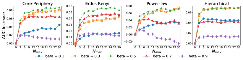
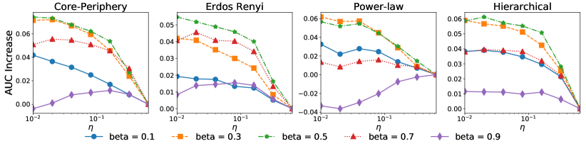
We now test the impact of changing (the threshold on nodes’ influence) or (maximum allowed nodes) of DAGs on the quality of inferred values.
We iterate over an increasing with a fixed RR’s across synthetic networks. Since we are interested in the change in resulting AUC scores and not their absolute values, we move each resulting curve so that their starting points would land on . Similarly for , we start from and exponentially grow the threshold to while is fixed. To make it easier to observe the change in AUC scores, we collocate the ending point of all curves on .
The results for and are depicted in Figures 1 and 2 respectively. Intuitively, one might expect that larger DAGs will always lead to more accurate results, albeit with some additional computational cost. This is almost true in both experiments. Interestingly, in some of the networks when the perturbation is minimal (), the quality actually drops as DAGs grow larger. This means that having a more selective DAG, with more restrictive criteria, can sometimes yield better results.
VI-F Who is More Vulnerable?
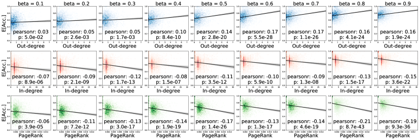
The AUC value describes the effectiveness of our inference algorithm but does not provide details on individual vertex level. Here we look into attributes that can indicate a node’s vulnerability to such an inference attack. Without access to ground truth values of , finding the best cutoff threshold of for classification is not possible. As an alternative, we calculate the expected accuracy of a single node’s inferred value if the threshold is selected at random from :
| (23) |
where is an indicator function. Note that we are not interested in the absolute values of , but the relative difference between different nodes, in order to compare nodes’ vulnerability to our attack.
We tested node attributes related to the centrality and importance of a node in a complex network: (1) (Weighted) Out-degree, (2) (Weighted) In-degree, and (3) PageRank [36]. We limit our visualizations to Core-Periphery networks due to limited space. Results are similar for the other 3 networks. We test values of and infer the real values using CO-DAG. In Figure 3 the resulting for each node is plotted against the metrics mentioned above along with correlation analysis printed on each plot. Each column contains plots with a similar value, printed on the top. Among the metrics, two of them (in-degree and PageRank) show a negative correlation, while a strong correlation is observed between and out-degree which grows even stronger as is increased and the added noise becomes minimal. A reasonable explanation is that when has a high impact on many nodes in the network, it essentially sends signals of its true value to those nodes during the spread of the contagion. These signals, each insignificant on its own, can collectively reveal the true value of to a great extent. Of course, these signals only grow stronger when the amount of added noise to each report is reduced as grows bigger. In contrast, there might be many signals on the influence received by a node with a high in-degree, but without that influence spreading around, we only have the report by that node as a single indicator of its true value which is masked well by conventional privacy protection techniques.
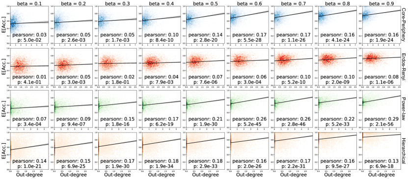
We repeat this experiment on other synthetic networks to see if we observe similar results. In Figure 4, is plotted against out-degree of all nodes for between and . A similar trend is visible across all types of network, with different intensity. In the networks where the distribution of influence is skewed, namely Core-Periphery, Power-law and Hierarchical, the correlation is strong. Moreover, as increases and the added noise become smaller, the correlation grows stronger. In Erdos-Renyi networks, where degrees are distributed more evenly, the difference in among nodes is minor and as a result, the correlation is weaker. Notice that in Hierarchical network, this unequal distribution of influence reaches its extreme point, where the majority of the nodes are leaves, with no impact on others, while a handful of nodes at the top influence many others. This radical difference leads to a constant unbalance between of the two groups across all values of .
VII Conclusion and Future Work
In this work, we provide further evidence that a privacy-protecting measure that is oblivious to socially contagious properties of attributes is unlikely to provide guarantees in practice as advertised. There are two obvious directions for future research: 1) design a privacy protection mechanism that is aware of the contagious property of some attributes and employs models of contagions in its design; Our method can be used to test if that method succeeds. 2) extend the results to other contagion models. Notice that the extension to any progressive contagion model (where active nodes stay active) with a differentiable formula (e.g, Independent Cascade model) is easily possible. However, ideas specific to those models are required for efficient implementation and model design.
Acknowledgement
Aria Rezaei and Jie Gao acknowledge support through NSF DMS-1737812, NSF CNS-1618391 and NSF CCF-1535900.
References
- [1] C. Dwork and A. Roth, “The algorithmic foundations of differential privacy,” Found. Trends Theor. Comput. Sci., vol. 9, no. 3–4, pp. 211–407, 2014.
- [2] E. Cohen-Cole and J. M. Fletcher, “Is obesity contagious? social networks vs. environmental factors in the obesity epidemic,” J. Health Econ., vol. 27, no. 5, pp. 1382–1387, Sep. 2008.
- [3] J. Hamari and J. Koivisto, ““working out for likes”: An empirical study on social influence in exercise gamification,” Comput. Human Behav., vol. 50, pp. 333–347, Sep. 2015.
- [4] R. M. Bond, C. J. Fariss, J. J. Jones, A. D. I. Kramer, C. Marlow, J. E. Settle, and J. H. Fowler, “A 61-million-person experiment in social influence and political mobilization,” Nature, vol. 489, no. 7415, pp. 295–298, Sep. 2012.
- [5] J. Meer, “Brother, can you spare a dime? peer pressure in charitable solicitation,” J. Public Econ., vol. 95, no. 7, pp. 926–941, Aug. 2011.
- [6] D. Wang, D. Pedreschi, C. Song, F. Giannotti, and A.-L. Barabasi, “Human mobility, social ties, and link prediction,” in Proceedings of the 17th ACM SIGKDD international conference on Knowledge discovery and data mining, Aug. 2011, pp. 1100–1108.
- [7] J. Gao, G. Ghasemiesfeh, G. Schoenebeck, and F.-Y. Yu, “General threshold model for social cascades: Analysis and simulations,” in Proceedings of the 2016 ACM Conference on Economics and Computation, Jul. 2016, pp. 617–634.
- [8] M. S. Granovetter, “The strength of weak ties,” Am. J. Sociol., vol. 78, no. 6, pp. 1360–1380, 1973.
- [9] D. Centola and M. Macy, “Complex contagions and the weakness of long ties,” Am. J. Sociol., vol. 113, no. 3, pp. 702–734, Nov. 2007.
- [10] G. Ghasemiesfeh, R. Ebrahimi, and J. Gao, “Complex contagion and the weakness of long ties in social networks: Revisited,” in Proceedings of the Fourteenth ACM Conference on Electronic Commerce, 2013, pp. 507–524.
- [11] D. Kifer and A. Machanavajjhala, “Pufferfish: A framework for mathematical privacy definitions,” ACM Trans. Database Syst., vol. 39, no. 1, pp. 3:1–3:36, Jan. 2014.
- [12] A. Ghosh and R. Kleinberg, “Inferential privacy guarantees for differentially private mechanisms,” Mar. 2016.
- [13] V. Rastogi, M. Hay, G. Miklau, and D. Suciu, “Relationship privacy: Output perturbation for queries with joins,” in Proceedings of the Twenty-eighth ACM SIGMOD-SIGACT-SIGART Symposium on Principles of Database Systems, 2009, pp. 107–116.
- [14] D. Kempe, J. Kleinberg, and É. Tardos, “Maximizing the spread of influence through a social network,” in Proceedings of the ninth ACM SIGKDD international conference on Knowledge discovery and data mining, 2003, pp. 137–146.
- [15] W. Chen, Y. Yuan, and L. Zhang, “Scalable influence maximization in social networks under the linear threshold model,” in 2010 IEEE International Conference on Data Mining, Dec. 2010, pp. 88–97.
- [16] C. Borgs, M. Brautbar, J. Chayes, and B. Lucier, “Maximizing social influence in nearly optimal time,” in Proceedings of the Twenty-Fifth Annual ACM-SIAM Symposium on Discrete Algorithms, Dec. 2013, pp. 946–957.
- [17] T. Lappas, E. Terzi, D. Gunopulos, and H. Mannila, “Finding effectors in social networks,” in Proceedings of the 16th ACM SIGKDD international conference on Knowledge discovery and data mining, 2010, pp. 1059–1068.
- [18] W. Luo, W. P. Tay, and M. Leng, “Identifying infection sources and regions in large networks,” IEEE Trans. Signal Process., vol. 61, no. 11, pp. 2850–2865, Jun. 2013.
- [19] H. T. Nguyen, P. Ghosh, M. L. Mayo, and T. N. Dinh, “Multiple infection sources identification with provable guarantees,” in Proceedings of the 25th ACM International on Conference on Information and Knowledge Management, Oct. 2016, pp. 1663–1672.
- [20] B. A. Prakash, J. Vreeken, and C. Faloutsos, “Spotting culprits in epidemics: How many and which ones?” in 2012 IEEE 12th International Conference on Data Mining, Dec. 2012, pp. 11–20.
- [21] C. Task and C. Clifton, “A guide to differential privacy theory in social network analysis,” in 2012 IEEE/ACM International Conference on Advances in Social Networks Analysis and Mining, Aug. 2012, pp. 411–417.
- [22] D. Kifer and A. Machanavajjhala, “No free lunch in data privacy,” in Proceedings of the 2011 ACM SIGMOD International Conference on Management of Data, 2011, pp. 193–204.
- [23] S. Song, Y. Wang, and K. Chaudhuri, “Pufferfish privacy mechanisms for correlated data,” in Proceedings of the 2017 ACM International Conference on Management of Data, 2017, pp. 1291–1306.
- [24] T. Fawcett, “An introduction to roc analysis,” Pattern recognition letters, vol. 27, no. 8, pp. 861–874, 2006.
- [25] J. A. Hanley and B. J. McNeil, “The meaning and use of the area under a receiver operating characteristic (roc) curve.” Radiology, vol. 143, no. 1, pp. 29–36, 1982.
- [26] C. Wang, W. Chen, and Y. Wang, “Scalable influence maximization for independent cascade model in large-scale social networks,” Data Mining and Knowledge Discovery, vol. 25, no. 3, pp. 545–576, 2012.
- [27] A. Goyal, W. Lu, and L. V. Lakshmanan, “Simpath: An efficient algorithm for influence maximization under the linear threshold model,” in 2011 IEEE 11th international conference on data mining, 2011, pp. 211–220.
- [28] M. Gomez-Rodriguez, J. Leskovec, and A. Krause, “Inferring networks of diffusion and influence,” ACM Transactions on Knowledge Discovery from Data (TKDD), vol. 5, no. 4, p. 21, 2012.
- [29] J. Leskovec, D. Chakrabarti, J. Kleinberg, C. Faloutsos, and Z. Ghahramani, “Kronecker graphs: An approach to modeling networks,” Journal of Machine Learning Research, vol. 11, no. Feb, pp. 985–1042, 2010.
- [30] M. E. Newman, “The structure and function of complex networks,” SIAM review, vol. 45, no. 2, pp. 167–256, 2003.
- [31] A. Clauset, C. Moore, and M. E. Newman, “Hierarchical structure and the prediction of missing links in networks,” Nature, vol. 453, no. 7191, p. 98, 2008.
- [32] J. Leskovec, J. Kleinberg, and C. Faloutsos, “Graph evolution: Densification and shrinking diameters,” ACM Transactions on Knowledge Discovery from Data (TKDD), vol. 1, no. 1, p. 2, 2007.
- [33] J. Leskovec, L. A. Adamic, and B. A. Huberman, “The dynamics of viral marketing,” ACM Transactions on the Web (TWEB), vol. 1, no. 1, p. 5, 2007.
- [34] A. Rezaei, B. Perozzi, and L. Akoglu, “Ties that bind: Characterizing classes by attributes and social ties,” in Proceedings of the 26th International Conference on World Wide Web Companion, 2017, pp. 973–981.
- [35] S. L. Warner, “Randomized response: A survey technique for eliminating evasive answer bias,” Journal of the American Statistical Association, vol. 60, no. 309, pp. 63–69, 1965.
- [36] L. Page, S. Brin, R. Motwani, and T. Winograd, “The pagerank citation ranking: Bringing order to the web.” Stanford InfoLab, Tech. Rep., 1999.