Classification Betters Regression in Query-based Multi-document Summarisation Techniques for Question Answering

Abstract

Task B Phase B of the 2019 BioASQ challenge focuses on biomedical question answering. Macquarie University’s participation applies query-based multi-document extractive summarisation techniques to generate a multi-sentence answer given the question and the set of relevant snippets. In past participation we explored the use of regression approaches using deep learning architectures and a simple policy gradient architecture. For the 2019 challenge we experiment with the use of classification approaches with and without reinforcement learning. In addition, we conduct a correlation analysis between various ROUGE metrics and the BioASQ human evaluation scores.

1 Introduction

The BioASQ Challenge includes a question answering task (Phase B, part B) where the aim is to find the “ideal answer” — that is, an answer that would normally be given by a person [12]. This is in contrast with most other question answering challenges where the aim is normally to give an exact answer, usually a fact-based answer or a list. Given that the answer is based on an input that consists of a biomedical question and several relevant PubMed abstracts, the task can be seen as an instance of query-based multi-document summarisation.

As in past participation [6, 7], we wanted to test the use of deep learning and reinforcement learning approaches for extractive summarisation. In contrast with past years where the training procedure was based on a regression set up, this year we experiment with various classification set ups. The main contributions of this paper are:

1. We compare classification and regression approaches and show that classification produces better results than regression but the quality of the results depends on the approach followed to annotate the data labels.

2. We conduct correlation analysis between various ROUGE evaluation metrics and the human evaluations conducted at BioASQ and show that Precision and F1 correlate better than Recall.

Section 2 briefly introduces some related work for context. Section 3 describes our classification and regression experiments. Section 4 details our experiments using deep learning architectures. Section 5 explains the reinforcement learning approaches. Section 6 shows the results of our correlation analysis between ROUGE scores and human annotations. Section 7 lists the specific runs submitted at BioASQ 7b. Finally, Section 8 concludes the paper.

2 Related Work

The BioASQ challenge has organised annual challenges on biomedical semantic indexing and question answering since 2013 [12]. Every year there has been a task about semantic indexing (task a) and another about question answering (task b), and occasionally there have been additional tasks. The tasks defined for 2019 are:

BioASQ Task 7a:

Large Scale Online Biomedical Semantic Indexing.

BioASQ Task 7b:

Biomedical Semantic QA involving Information Retrieval (IR), Question Answering (QA), and Summarisation.

BioASQ MESINESP Task:

Medical Semantic Indexing in Spanish.

BioASQ Task 7b consists of two phases. Phase A provides a biomedical question as an input, and participants are expected to find relevant concepts from designated terminologies and ontologies, relevant articles from PubMed, relevant snippets from the relevant articles, and relevant RDF triples from designated ontologies. Phase B provides a biomedical question and a list of relevant articles and snippets, and participant systems are expected to return the exact answers and the ideal answers. The training data is composed of the test data from all previous years, and amounts to 2,747 samples.

There has been considerable research on the use of machine learning approaches for tasks related to text summarisation, especially on single-document summarisation. Abstractive approaches normally use an encoder-decoder architecture and variants of this architecture incorporate attention [10] and pointer-generator [11]. Recent approaches leveraged the use of pre-trained models [2]. Recent extractive approaches to summarisation incorporate recurrent neural networks that model sequences of sentence extractions [8] and may incorporate an abstractive component and reinforcement learning during the training stage [13]. But relatively few approaches have been proposed for query-based multi-document summarisation. Table 1 summarises the approaches presented in the proceedings of the 2018 BioASQ challenge.

Table 1: Summarisation techniques used in BioASQ 6b for the generation of ideal answers. The evaluation result is the human evaluation of the best run.

System	Abstractive Approaches	Extractive Approaches
[7]	(none)	Regression & Reinforcement Learning
[4]	Fusion	Maximum Marginal Relevance
[1]	(none)	Lexical chains
[9]	Fine-tuned Pointer Generator Coverage	Learning to rank

3 Classification vs. Regression Experiments

Our past participation in BioASQ [6, 7] and this paper focus on extractive approaches to summarisation. Our decision to focus on extractive approaches is based on the observation that a relatively large number of sentences from the input snippets has very high ROUGE scores, thus suggesting that human annotators had a general tendency to copy text from the input to generate the target summaries [6]. Our past participating systems used regression approaches using the following framework:

1. Train the regressor to predict the ROUGE-SU4 F1 score of the input sentence.

2. Produce a summary by selecting the top $n$ input sentences.

A novelty in the current participation is the introduction of classification approaches using the following framework.

1. Train the classifier to predict the target label (“summary” or “not summary”) of the input sentence.

2. Produce a summary by selecting all sentences predicted as “summary”.

3. If the total number of sentences selected is less than $n$, select $n$ sentences with higher probability of label “summary”.

Introducing a classifier makes labelling the training data not trivial, since the target summaries are human-generated and they do not have a perfect mapping to the input sentences. In addition, some samples have multiple reference summaries. [3] showed that different data labelling approaches influence the quality of the final summary, and some labelling approaches may lead to better results than using regression. In this paper we experiment with the following labelling approaches:

threshold $t$

: Label as “summary” all sentences from the input text that have a ROUGE score above a threshold $t$.

top $m$

: Label as “summary” the $m$ input text sentences with highest ROUGE score.

As in [3], The ROUGE score of an input sentence was the ROUGE-SU4 F1 score of the sentence against the set of reference summaries.

We conducted cross-validation experiments using various values of $t$ and $m$. Table 3 shows the results for the best values of $t$ and $m$ obtained. The regressor and classifier used Support Vector Regression (SVR) and Support Vector Classification (SVC) respectively. To enable a fair comparison we used the same input features in all systems. These input features combine information from the question and the input sentence and are shown in Fig. 1. The features are based on [5], and are the same as in [6], plus the addition of the position of the input snippet. The best SVC and SVR parameters were determined by grid search.

• $tf.idf$ vector of the candidate sentence.

• Cosine similarity between the $tf.idf$ vector of the question and the $tf.idf$ vector of the candidate sentence.

• The largest cosine similarity between the $tf.idf$ vector of candidate sentence and the $tf.idf$ vector of each of the snippets related to the question.

• Cosine similarity between the sum of word2vec embeddings of the words in the question and the word2vec embeddings of the words in the candidate sentence. We used vectors of dimension 200 pre-trained using PubMed documents provided by the organisers of BioASQ.

• Pairwise cosine similarities between the words of the question and the words of the candidate sentence. We used word2vec to compute the word vectors. We then computed the pairwise cosine similarities and selected the following features:

  • The mean, median, maximum, and minimum of all pairwise cosine similarities.

  • The mean of the 2 highest, mean of the 3 highest, mean of the 2 lowest, and mean of the 3 lowest.

• Weighted pairwise cosine similarities where the weight was the $tf.idf$ of the word.

Figure 1: Features used in the SVC and SVR experiments.

Preliminary experiments showed a relatively high number of cases where the classifier did not classify any of the input sentences as “summary”. To solve this problem, and as mentioned above, the summariser used in Table 3 introduces a backoff step that extracts the $n$ sentences with highest predicted values when the summary has less than $n$ sentences. The value of $n$ is as reported in our prior work and shown in Table 2.

Table 2: Number of sentences returned by the regression-based summarisers and the backoff step of the classification-based summarisers, for each question type

	Summary	Factoid	Yesno	List
n	6	2	2	3

The results confirm [3]’s finding that classification outperforms regression. However, the actual choice of optimal labelling scheme was different: whereas in [3] the optimal labelling was based on a labelling threshold of 0.1, our experiments show a better result when using the top 5 sentences as the target summary. The reason for this difference might be the fact that [3] used all sentences from the abstracts of the relevant PubMed articles, whereas we use only the snippets as the input to our summariser. Consequently, the number of input sentences is now much smaller. We therefore report the results of using the labelling schema of top 5 snippets in all subsequent classifier-based experiments of this paper.

Table 3: Regression vs. classification approaches measured using ROUGE SU4 F-score under 10-fold cross-validation. The table shows the mean and standard deviation across the folds. “firstn” is a baseline that selects the first n sentences. SVR and SVC are described in Section 3. NNR and NNC are described in Section 4.

Method	Labelling	ROUGE-SU4 F1
		Mean $\pm$	1 stdev
firstn		0.252 $\pm$	0.015
SVR	SU4 F1	0.239 $\pm$	0.009
SVC	threshold 0.2	0.240 $\pm$	0.012
SVC	top 5	0.253 $\pm$	0.013
NNR	SU4 F1	0.254 $\pm$	0.013
NNC	SU4 F1	0.257 $\pm$	0.012
NNC	top 5	0.262 $\pm$	0.012

4 Deep Learning Models

Based on the findings of Section 3, we apply minimal changes to the deep learning regression models of [7] to convert them to classification models. In particular, we add a sigmoid activation to the final layer, and use cross-entropy as the loss function. The complete architecture is shown in Fig. 2.

Figure 2: Architecture of the neural classification and regression systems. A matrix of pre-trained word embeddings (same pre-trained vectors as in Fig. 1) is used to find the embeddings of the words of the input sentence and the question. Then, LSTM chains are used to generate sentence embeddings — the weights of the LSTM chains of input sentence and question are not shared. Then, the sentence position is concatenated to the sentence embedding and the similarity of sentence and question embeddings, implemented as a product. A final layer predicts the label of the sentence.

The bottom section of Table 3 shows the results of several variants of the neural architecture. The table includes a neural regressor (NNR) and a neural classifier (NNC). The neural classifier is trained in two set ups: “NNC top 5” uses classification labels as described in Section 3, and “NNC SU4 F1” uses the regression labels, that is, the ROUGE-SU4 F1 scores of each sentence. Of interest is the fact that “NNC SU4 F1” outperforms the neural regressor. We have not explored this further and we presume that the relatively good results are due to the fact that ROUGE values range between 0 and 1, which matches the full range of probability values that can be returned by the sigmoid activation of the classifier final layer.

Table 3 also shows the standard deviation across the cross-validation folds. Whereas this standard deviation is fairly large compared with the differences in results, in general the results are compatible with the top part of the table and prior work suggesting that classification-based approaches improve over regression-based approaches.

5 Reinforcement Learning

We also experiment with the use of reinforcement learning techniques. Again these experiments are based on [7], who uses REINFORCE to train a global policy. The policy predictor uses a simple feedforward network with a hidden layer.

The results reported by [7] used ROUGE Recall and indicated no improvement with respect to deep learning architectures. Human evaluation results are preferable over ROUGE but these were made available after the publication of the paper. When comparing the ROUGE and human evaluation results (Table 4), we observe an inversion of the results. In particular, the reinforcement learning approaches (RL) of [7] receive good human evaluation results, and as a matter of fact they are the best of our runs in two of the batches. In contrast, the regression systems (NNR) fare relatively poorly. Section 6 expands on the comparison between the ROUGE and human evaluation scores.

Table 4: Results of ROUGE-SU4 Recall (R) and human (H) evaluations on BioASQ 6b runs, batch 5. The human evaluation shows the average of all human evaluation metrics.

Run	System	Batch 1		Batch 2		Batch 3		Batch 4		Batch 5
		R	H	R	H	R	H	R	H	R	H
MQ-1	First $n$	0.46	3.91	0.50	4.01	0.45	4.06	0.51	4.16	0.59	4.05
MQ-2	Cosine	0.52	3.96	0.50	3.97	0.45	3.97	0.53	4.15	0.59	4.06
MQ-3	SVR	0.49	3.87	0.51	3.96	0.49	4.06	0.52	4.17	0.62	3.98
MQ-4	NNR	0.55	3.85	0.54	3.93	0.51	4.05	0.56	4.19	0.64	4.02
MQ-5	RL	0.38	3.92	0.43	4.01	0.38	4.04	0.46	4.18	0.52	4.14

Encouraged by the results of Table 4, we decided to continue with our experiments with reinforcement learning. We use the same features as in [7], namely the length (in number of sentences) of the summary generated so far, plus the $tf.idf$ vectors of the following:

1. Candidate sentence;

2. Entire input to summarise;

3. Summary generated so far;

4. Candidate sentences that are yet to be processed; and

5. Question.

The reward used by REINFORCE is the ROUGE value of the summary generated by the system. Since [7] observed a difference between the ROUGE values of the Python implementation of ROUGE and the original Perl version (partly because the Python implementation does not include ROUGE-SU4), we compare the performance of our system when trained with each of them. Table 5 summarises some of our experiments. We ran the version trained on Python ROUGE once, and the version trained on Perl twice. The two Perl runs have different results, and one of them clearly outperforms the Python run. However, given the differences of results between the two Perl runs we advice to re-run the experiments multiple times and obtain the mean and standard deviation of the runs before concluding whether there is any statistical difference between the results. But it seems that there may be an improvement of the final evaluation results when training on the Perl ROUGE values, presumably because the final evaluation results are measured using the Perl implementation of ROUGE.

Table 5: Experiments using Perl and Python versions of ROUGE. The Python version used the average of ROUGE-2 and ROUGE-L, whereas the Perl version used ROUGE-SU4.

Training on	Python ROUGE	Perl ROUGE
Python implementation	0.316	0.259
Perl implementation 1	0.287	0.238
Perl implementation 2	0.321	0.274

We have also tested the use of word embeddings instead of $tf.idf$ as input features to the policy model, while keeping the same neural architecture for the policy (one hidden layer using the same number of hidden nodes). In particular, we use the mean of word embeddings using 100 and 200 dimensions. These word embeddings were pre-trained using word2vec on PubMed documents provided by the organisers of BioASQ, as we did for the architectures described in previous sections. The results, not shown in the paper, indicated no major improvement, and re-runs of the experiments showed different results on different runs. Consequently, our submission to BioASQ included the original system using $tf.idf$ as input features in all batches but batch 2, as described in Section 7.

6 Evaluation Correlation Analysis

As mentioned in Section 5, there appears to be a large discrepancy between ROUGE Recall and the human evaluations. This section describes a correlation analysis between human and ROUGE evaluations using the runs of all participants to all previous BioASQ challenges that included human evaluations (Phase B, ideal answers). The human evaluation results were scraped from the BioASQ Results page, and the ROUGE results were kindly provided by the organisers. We compute the correlation of each of the ROUGE metrics (recall, precision, F1 for ROUGE-2 and ROUGE-SU4) against the average of the human scores. The correlation metrics are Pearson, Kendall, and a revised Kendall correlation explained below.

The Pearson correlation between two variables is computed as the covariance of the two variables divided by the product of their standard deviations. This correlation is a good indication of a linear relation between the two variables, but may not be very effective when there is non-linear correlation.

The Spearman rank correlation and the Kendall rank correlation are two of the most popular among metrics that aim to detect non-linear correlations. The Spearman rank correlation between two variables can be computed as the Pearson correlation between the rank values of the two variables, whereas the Kendall rank correlation measures the ordinal association between the two variables using Equation 1.

$$\tau=\frac{(\hbox{number of concordant pairs})-(\hbox{number of discordant pairs})}{n(n-1)/2}$$ (1)

It is useful to account for the fact that the results are from 28 independent sets (3 batches in BioASQ 1 and 5 batches each year between BioASQ 2 and BioASQ 6). We therefore also compute a revised Kendall rank correlation measure that only considers pairs of variable values within the same set. The revised metric is computed using Equation 2, where $S$ is the list of different sets.

$$\tau^{\prime}=\frac{\sum_{i\in S}\left[(\hbox{number of concordant pairs})_{i}-(\hbox{number of discordant pairs})_{i}\right]}{\sum_{i\in S}\left[n_{i}(n_{i}-1)/2\right]}$$ (2)

Table 6 shows the results of all correlation metrics. Overall, ROUGE-2 and ROUGE-SU4 give similar correlation values but ROUGE-SU4 is marginally better. Among precision, recall and F1, both precision and F1 are similar, but precision gives a better correlation. Recall shows poor correlation, and virtually no correlation when using the revised Kendall measure. For reporting the evaluation of results, it will be therefore more useful to use precision or F1. However, given the small difference between precision and F1, and given that precision may favour short summaries when used as a function to optimise in a machine learning setting (e.g. using reinforcement learning), it may be best to use F1 as the metric to optimise.

Table 6: Correlation analysis of evaluation results

Metric	Pearson	Spearman	Kendall	Revised Kendall
ROUGE-2 precision	0.61	0.78	0.58	0.73
ROUGE-2 recall	0.41	0.24	0.16	-0.01
ROUGE-2 F1	0.62	0.68	0.49	0.42
ROUGE-SU4 precision	0.61	0.79	0.59	0.74
ROUGE-SU4 recall	0.40	0.20	0.13	-0.02
ROUGE-SU4 F1	0.63	0.69	0.50	0.43

Fig. 3 shows the scatterplots of ROUGE-SU4 recall, precision and F1 with respect to the average human evaluation. We observe that the relation between ROUGE and the human evaluations is not linear, and that Precision and F1 have a clear correlation.

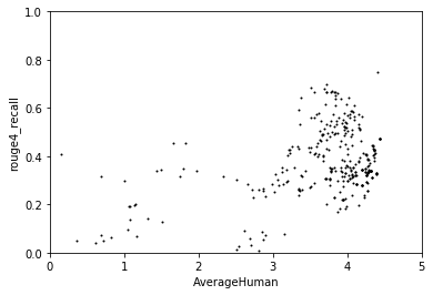
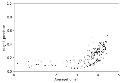
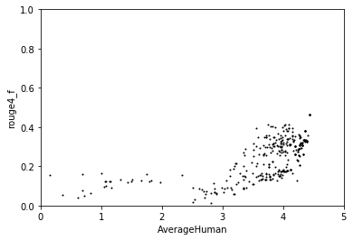
Figure 3: Scatterplots of ROUGE SU4 evaluation metrics against the average human evaluations.

7 Submitted Runs

Table 7 shows the results and details of the runs submitted to BioASQ. The table uses ROUGE-SU4 Recall since this is the metric available at the time of writing this paper. However, note that, as explained in Section 6, these results might differ from the final human evaluation results. Therefore we do not comment on the results, other than observing that the “first $n$” baseline produces the same results as the neural regressor. As mentioned in Section 3, the labels used for the classification experiments are the 5 sentences with highest ROUGE-SU4 F1 score.

Table 7: Runs submitted to BioASQ 7b

Batch	Run	Description	ROUGE-SU4 R
1	MQ1	First $n$	0.4741
	MQ2	SVC	0.5156
	MQ3	NNR batchsize=4096	0.4741
	MQ4	NNC batchsize=4096	0.5214
	MQ5	RL tf.idf & Python ROUGE	0.4616
2	MQ1	First $n$	0.5113
	MQ2	SVC	0.5206
	MQ3	NNR batchsize=4096	0.5113
	MQ4	NNC batchsize=4096	0.5337
	MQ5	RL embeddings 200 & Python ROUGE	0.4787
3	MQ1	First $n$	0.4263
	MQ2	SVC	0.4512
	MQ3	NNR batchsize=4096	0.4263
	MQ4	NNC batchsize=4096	0.4782
	MQ5	RL tf.idf & Python ROUGE	0.4189
4	MQ1	First $n$	0.4617
	MQ2	SVC	0.4812
	MQ3	NNR batchsize=1024	0.4617
	MQ4	NNC batchsize=1024	0.5246
	MQ5	RL tf.idf & Python ROUGE	0.3940
5	MQ1	First $n$	0.4952
	MQ2	SVC	0.5024
	MQ3	NNR batchsize=1024	0.4952
	MQ4	NNC batchsize=1024	0.5070
	MQ5	RL tf.idf & Perl ROUGE	0.4520

8 Conclusions

Macquarie University’s participation in BioASQ 7 focused on the task of generating the ideal answers. The runs use query-based extractive techniques and we experiment with classification, regression, and reinforcement learning approaches. At the time of writing there were no human evaluation results, and based on ROUGE-F1 scores under cross-validation on the training data we observed that classification approaches outperform regression approaches. We experimented with several approaches to label the individual sentences for the classifier and observed that the optimal labelling policy for this task differed from prior work.

We also observed poor correlation between ROUGE-Recall and human evaluation metrics and suggest to use alternative automatic evaluation metrics with better correlation, such as ROUGE-Precision or ROUGE-F1. Given the nature of precision-based metrics which could bias the system towards returning short summaries, ROUGE-F1 is probably more appropriate when using at development time, for example for the reward function used by a reinforcement learning system.

Reinforcement learning gives promising results, especially in human evaluations made on the runs submitted to BioASQ 6b. This year we introduced very small changes to the runs using reinforcement learning, and will aim to explore more complex reinforcement learning strategies and more complex neural models in the policy and value estimators.

References

- [1] Bhandwaldar, A., Charlotte, U.N.C., Charlotte, U.N.C.: UNCC QA : A Biomedical Question Answering System. In: Proceedings BioASQ Workshop at EMNLP 2018. pp. 66–71 (2018)
- [2] Hoang, A., Bosselut, A., Celikyilmaz, A., Choi, Y.: Efficient Adaptation of Pretrained Transformers for Abstractive Summarization. Arxiv pre-print 1906.00138 (may 2019)
- [3] Kaur, M., Mollá, D.: Supervised Machine Learning for Extractive Query Based Summarisation of Biomedical Data. In: Proc. Louhi 2018 (2018)
- [4] Li, Y., Gekakis, N., Chandu, K.R., Nyberg, E.: Extraction Meets Abstraction : Ideal Answer Generation for Biomedical Questions. In: Proceedings BioASQ Workshop at EMNLP 2018. pp. 57–65 (2018)
- [5] Malakasiotis, P., Archontakis, E., Androutsopoulos, I.: Biomedical question-focused multi-document summarization : ILSP and AUEB at BioASQ3. In: CLEF 2015 Working Notes (2015)
- [6] Mollá, D.: Macquarie University at BioASQ 5b — Query-based Summarisation Techniques for Selecting the Ideal Answers. In: Proc. BioNLP2017 (2017)
- [7] Mollá, D.: Macquarie University at BioASQ 6b: Deep learning and deep reinforcement learning for query-based multi-document summarisation. In: Proceedings BioASQ Workshop at EMNLP 2018 (2018)
- [8] Nallapati, R., Zhai, F., Zhou, B.: SummaRuNNer: A Recurrent Neural Network based Sequence Model for Extractive Summarization of Documents. In: AAAI 2017 (nov 2017)
- [9] Naresh Kumar, A., Kesavamoorthy, H., Das, M., Kalwad, P., Raghavi Chandu, K., Mitamura, T., Nyberg, E.: Ontology-Based Retrieval & Neural Approaches for BioASQ Ideal Answer Generation. In: Proceedings BioASQ Workshop at EMNLP 2018. pp. 79–89 (2018)
- [10] Rush, A.M., Chopra, S., Weston, J.: A Neural Attention Model for Abstractive Sentence Summarization. In: In Proceedings of the Conference on Empirical Methods in Natural Language Processing (EMNLP). pp. 379–389. No. September (2015)
- [11] See, A., Liu, P.J., Manning, C.D.: Get To The Point: Summarization with Pointer-Generator Networks. In: ACL 2017 (2017)
- [12] Tsatsaronis, G., Balikas, G., Malakasiotis, P., Partalas, I., Zschunke, M., Alvers, M.R., Weissenborn, D., Krithara, A., Petridis, S., Polychronopoulos, D., Almirantis, Y., Pavlopoulos, J., Baskiotis, N., Gallinari, P., Artiéres, T., Ngomo, A.C.N., Heino, N., Gaussier, E., Barrio-Alvers, L., Schroeder, M., Androutsopoulos, I., Paliouras, G.: An Overview of the BIOASQ Large-Scale Biomedical Semantic Indexing and Question Answering Competition. BMC Bioinformatics 16(1), 138 (2015). https://doi.org/10.1186/s12859-015-0564-6
- [13] Zhang, X., Lapata, M., Wei, F., Zhou, M.: Neural Latent Extractive Document Summarization. In: EMNLP 2018 (aug 2018)