Can A User Anticipate What Her Followers Want?
Abstract
Whenever a social media user decides to share a story, she is typically pleased to receive likes, comments, shares, or, more generally, feedback from her followers. As a result, she may feel compelled to use the feedback she receives to (re-)estimate her followers’ preferences and decide which stories to share next to receive more (positive) feedback. Under which conditions can she succeed? In this work, we first look into this problem from a theoretical perspective and then provide a set of practical algorithms to identify and characterize such behavior in social media.
More specifically, we address the above problem from the perspective of sequential decision making and utility maximization. For a wide variety of utility functions, we first show that, to succeed, a user requires to actively trade off exploitation—sharing stories which lead to more (positive) feedback—and exploration—sharing stories to learn about her followers’ preferences. However, exploration is not necessary if a user utilizes the feedback her followers provide to other users in addition to the feedback she receives. Then, we develop a utility estimation framework for observation data, which relies on statistical hypothesis testing to determine whether a user utilizes the feedback she receives from each of her followers to decide what to post next. Experiments on synthetic data illustrate our theoretical findings and show that our estimation framework is able to accurately recover users’ underlying utility functions. Experiments on several real datasets gathered from Twitter and Reddit reveal that up to % (%) of the Twitter (Reddit) users in our datasets do use the feedback they receive to decide what to post next.
1 Introduction
Political parties, corporations, celebrities as well as ordinary people use social media to build, reach, and share stories with their own audience. For example, political leaders share details about their activities in hopes of tapping new voters [1], corporations offer insights about their latest products and services with potential customers [16], celebrities give a glimpse of their lavish lifestyle to strengthen their fan base [2], and ordinary people share personal stories with their friends [3]. In all these cases, social media users—politicians, corporations, celebrities, or ordinary people—receive feedback from their followers—their voters, customers, fans, or friends—by means of likes, comments, or shares. Moreover, this feedback provides hints about the preferences of their followers: it lets the users know what does or does not work, and it influences what they share next, as shown by an increasing number of empirical studies [21, 22, 17, 24, 15, 13, 11, 12, 19, 20]. In this context, it is perhaps surprising that feedback models of posting behavior are largely nonexistent to date. However, such models are of outstanding interest since they would allow us to answer two fundamental questions:
-
(i)
Can a user succeed at maximizing the (positive) feedback she receives if, a priori, does not know her followers’ preferences?
-
(ii)
Can we determine whether a user utilizes the feedback she receives from each of her followers to decide what to post next using observational data?
By answering the above questions, we will not only advance our understanding of how feedback may influence a user’s posting behavior but will also facilitate the design of more effective algorithms for viral marketing and user personalization.
1.1 Overview of our Approach
In this paper, we introduce a utility maximization feedback model of posting behavior, which is specially well-fitted to investigate the above questions. More specifically, we assume that each user has an underlying (linear) utility function, which assigns different weights to the feedback the user receives from each of her followers. Moreover, every time the user shares a story with her followers, they provide their feedback according to a set of preferences. If the user knows perfectly her followers’ preferences, we can then show that the optimal posting strategy, which maximizes the user’s utility function, is deterministic. If the user does not know their preferences, we have the following theoretical results:
-
I.
If the user estimates her followers’ preferences from the feedback she receives over time, she needs to resort to posting strategies that effectively trade-off exploitation—sharing stories to maximize her utility—and exploration—sharing stories to learn about her followers’ preferences. More formally, we can show that posterior sampling based posting strategies achieve logarithmic regret (i.e., ) while strategies based on point estimates suffer from linear regret (i.e., ) where denotes the total time steps.
-
II.
If the user can, in addition to the feedback she receives, also use the feedback her followers give to other users to estimate her followers’ preferences, she is better off using it. More specifically, we can show that posterior sampling based posting strategies achieve constant regret (i.e., ) and, perhaps surprisingly, strategies based on point estimates achieve sublinear regret (i.e., ).
In addition to the above theoretical analysis, we also develop a utility estimation framework, which relies on statistical hypothesis testing to determine whether a user utilizes the feedback she receives from each of her followers to decide what to post next. Finally, we perform a variety of experiments using both synthetic and real Twitter and Reddit data. Experiments on synthetic data illustrate our theoretical findings and show that our utility estimation framework is able to accurately recover the users’ underlying utility functions. Experiments on several real datasets gathered from Twitter and Reddit reveal that up to % (%) of the Twitter (Reddit) users in our datasets do use the feedback they receive to decide what to post next.
1.2 Related Work
In addition to the empirical studies on how feedback influences user behavior, discussed previously, our work also relates to revealed preference theory, smart broadcasting, and multi-armed bandits.
Revealed preference theory. Since the pioneering work by Samuelson [29], reveal preference theory has become a well-established economic theory that analyzes choices made by individuals, particularly to understand consumer behavior. It typically assumes that each consumer decides to buy a bundle of goods, among several alternatives, on the basis of a (concave) nondecreasing utility function [26, 27, 4]. The works most closely related to ours [10, 32, 18, 9, 7] aim to develop efficient algorithms to estimate utility functions from revealed preference data as well as analyze their sample complexity. However, their problem setting is very different from ours: (i) the utility a consumer obtains from buying a bundle of goods is deterministic, however, the feedback a social media user receives from her followers varies randomly and, thus, the utility a user obtains from sharing a story is stochastic; (ii) a consumer can evaluate the utility of a bundle of goods exactly, however, a social media user needs to guess the utility she will obtain from sharing a story on the basis of an estimation of her followers’ preferences from the feedback she received in the past; and, (iii) each consumer’s decision is independent, however, each social media user’s decision is part of a sequential decision making process.
Smart broadcasting. In recent years, there has been some work on smart broadcasting [30, 34, 25, 33], which aims to find the times when a user should post to receive more views, likes, comments, or shares from her followers. In smart broadcasting, there is also a user who aims to maximize the impact of the stories she shares, however, the focus is on when to share while our focus is on what to share. In addition, algorithms for smart broadcasting are based on temporal point processes and stochastic optimal control, while we resort to online learning techniques and convex optimization.
Multi-armed bandits. The proof techniques used for deriving regret bounds in bandit problems [5, 8, 23, 6] are related to the ones we use to derive the regret bounds in our work. However, there are several key differences: (i) we allow a user to utilize the feedback her followers provide to other users to estimate her followers’ preferences, whereas, in a traditional bandit setting, a user could only utilize the feedback she receives on the stories she shares; (ii) our proof techniques allow for users with several followers, in contrast, in a traditional bandit setting, it would only allow for users with one follower.
2 Feedback model of posting behavior
In this section, we introduce our feedback model of posting behavior, starting from the problem setting it is designed for.
2.1 Problem Setting
Let be a social media user and be her set of followers. Then, at each time , the user shares a story from a topic , with , and each of her followers decides whether to give (or not to give) feedback.111For simplicity, we assume that receiving feedback is always positive, e.g., we assume that receiving a like is always positive. Our formulation can be easily adapted to scenarios with positive and negative feedback, e.g., upvotes and downvotes. Moreover, for each follower , we denote the feedback she gave (or did not give) to user and, possibly, to any other user in the social media platform222We will study two scenarios: (i) the user has access only to the feedback she has received; and (ii) the user has access to the feedback she has received as well as the feedback her followers have given to other users., up to time by
where denotes the topic of the story, means that she gave feedback to the story and otherwise. We denote the collection of feedback from followers as .
At time , we assume that the user samples the topic of the story she shares from a categorical distribution , which may depend on the history of her followers’ feedback. Also, given a topic , each follower gives feedback with conditional probability , where we can think of as follower ’s preference for topic . Here, we assume that, in general, followers may differ in their preferences, i.e., for . Moreover, we denote and .
2.2 Utility Maximization Feedback Model
We assume that user aims to find (and utilize) the categorical distribution that maximizes a (linear) utility function , defined as
| (1) |
where the expectation is over the topics of the stories the user shares and the feedback . The weights model the importance that user gives to the feedback she receives from follower , the parameters encode user ’s preference for topic , the weight models the importance she gives to her own preferences, and we assume that . In the above utility function, the greater the importance user gives to the feedback she receives from a specific follower , the greater the utility gain she will obtain from posting a story from a topic that follower prefers. Similarly, the greater the importance she gives to her own preferences , the greater the utility gain she will obtain from just posting a story from a topic she prefers.
Next, using the linearity of expectation and the law of iterated expectation, we can rewrite Eq. 1 as follows:
| (2) |
where and denotes the transpose operator.
Finally, we can formally state the utility maximization problem user aims to solve as:
| (3) | ||||
| subject to | ||||
where the followers’ preferences are generally unknown.
3 Solving the utility maximization problem
In this section, we develop an efficient algorithm to solve the utility maximization problem defined by Eq. 3 and study its theoretical guarantees in a variety of settings.
3.1 Known Preferences
As a warm up, we first assume that the user knows her followers’ preferences . In this setting, it readily follows that the optimal distribution that maximizes Eq. 3 does not depend on the feedback history and is given by
| (4) |
where denotes the indicator function. In this case, note that the optimal mechanism for maximizing utility is deterministic (assuming ties over different topics are broken in a predetermined way).
3.2 Unknown Preferences: Exploration Exploitation Trade-off
In this section, we consider a more realistic setting where the user does not know the preferences . For this setting, we assume that the user can access historical feedback data to estimate these unknown preferences. When user does not know her followers’ preferences, she needs to trade off exploitation, i.e., maximizing utility, and exploration, i.e., learning about her followers’ preferences from historical feedback data.
To this aim, for every topic and follower , we assume a Beta prior over the preference parameter . Under this assumption, at each time , we can use to update the distribution of parameter as:
| (5) |
where
Then, at the beginning of time , we can estimate the value of each preference parameter in the following two ways:
-
I.
using point estimates, i.e.,
(6) -
II.
via sampling from posterior, i.e.,
(7)
Given these estimates, we select what to share next using an empirical approximation to Eq. 4, i.e.,
| (8) |
where . Algorithm 1 summarizes the complete procedure. Within the algorithm, Share shares a story from a given topic , GatherFeedback gathers the feedback from a follower , and Estimate returns an estimate of the preferences parameters using either point estimates or posterior samples.
3.3 Unknown Preferences: Analysis
In this section, we analyze the theoretical guarantees of Algorithm 1 in terms of regret , which we define as follows:
| (9) |
where is the utility achieved by Algorithm 1 and is the utility achieved by the optimal categorical distribution , given by Eq. 4, under the true preference parameters . Note that an algorithm is called a no-regret algorithm if the regret grows sublinearly (i.e., ) which implies that the algorithm’s average performance converges to that of the optimal algorithm.
Note that the utility depends on the quality of the estimates , which in turn depend on (i) the estimation method (i.e., point estimates vs posterior samples) and (ii) whether each follower’s feedback history only contains the feedback the follower gives to user or it also contains the feedback she gives to others. Next, we study several cases separately.
3.3.1 Point estimates
If the user only has access to the feedback she receives from her followers, we have the following negative result (proven in Appendix 8.1):
Theorem 1.
Assume user uses point estimates and she can only access the feedback she receives from her followers. Then, Algorithm 1 suffers linear regret .
Perhaps surprisingly, Algorithm 1 with point estimates can actually achieve sublinear regret if the user has access to both the feedback her followers give to her as well as to others, as formalized by the following theorem (proven in Appendix 8.2):
Theorem 2.
Assume user uses point estimates for the followers’ preferences and she can access both the feedback her followers give to her as well as to others. Furthermore, the amount of feedback each of her followers give to others per topic follows a Poisson distribution with rate , and let . Then, for , Algorithm 1 achieves regret
and, for , it achieves:
3.3.2 Posterior samples
If the user uses posterior samples, she is better off. In this case, Algorithm 1 achieves sublinear regret independently on whether contains only the feedback she receives or also the feedback her followers give to others. More formally, we have the following Theorem and Corollary (proven in Appendix 8.2):
Theorem 3.
Assume user uses posterior samples to estimate the followers’ preferences , she can access both the feedback her followers give to her as well as to others, and the amount of feedback each of her followers give to others per topic follows a Poisson distribution with rate . Then, Algorithm 1 has regret
where depends on the parameters in non-trivial way.
Corollary 4.
Assume user uses posterior samples to estimate the followers’ preferences and she can only access the feedback she receives from her followers. Then, Algorithm 1 has regret .
In summary, if user uses posterior samples instead of point estimates, she can effectively trade off exploitation—sharing stories for maximizing her utility—and exploration—sharing stories to estimate her followers’ preferences. Moreover, if she has access to the feedback that her neighbors provide to others, she is better off using it. Such additional information helps her to maximize her utility more effectively in both cases—posterior samples and point estimates.
4 Utility estimation framework
In this section, assume we observe both the stories user shared at each time and the feedback she received from her followers. Then, our goal is to determine whether the user utilizes the feedback she receives from each of her followers to decide what to post next. To this aim, we first find the model parameters that best fit the observed data and then determine its statistical significance using statistical hypothesis testing.
4.1 Parameter estimation
To find the weights and and parameters in Eq. 3 that best fit the observed data, one could resort to maximum likelihood estimation, i.e.,
| (10) | ||||
| subject to | ||||
where implicitly depends on and since it is the distribution that maximizes the utility function.
However, the above maximum likelihood estimation problem faces two serious challenges. First, it is stated in terms of either the optimal distribution or, in practice, . However, both distributions concentrate their entire probability mass in one topic. As a consequence, if there exists a time in which user shares a story from a topic that is not the optimal one to choose, the log-likelihood (or ) becomes unbounded. Fortunately, we can overcome this undesirable behavior by approximating the distribution (or ) using a softmax distribution
| (11) |
where is a given parameter and or . Second, if the number of feedback events is large, the above maximum likelihood estimation problem is not scalable. To ameliorate this second challenge, in the following, we present a highly efficient heuristic based on linear loss minimization.
Our starting point is the following intuition: at each time , if user is sampling the topic of the story she shares from a distribution that is close to , then the difference between the optimal topic and the observed topic, i.e.,
| (12) |
should be small. Therefore, our heuristic finds the weights and and the parameters that minimizes this difference over time. In practice, the solution to the above problem depends on whether we assume that the user utilized point estimates or posterior samples for the followers’ preferences. Therefore, we proceed in turn.
4.1.1 Point estimates
If we assume that the user utilized point estimates for her followers’ preferences, then we minimize:
| (13) |
However, the optimization problem is not convex due to the terms and, in its current form, it is difficult to solve efficiently. Fortunately, an invertible nonlinear transformation of the variables transforms it into a convex problem. Let and . Then, we can rewrite the optimization problem as:
| subject to | |||
which is a convex problem jointly in , , and using composition rules and the fact that the log-exp function is convex. Once we solve this convex problem, we can recover as .
4.1.2 Posterior samples
If we assume that the user utilized posterior samples for her followers’ preferences, then, we need to take the average of the objective function with respect to the posterior distributions of the followers’ preferences for all topics, since we do not know which sample the user actually took, i.e., the objective function becomes
where for all and . In practice, we just replace the above objective function by the empirical average with respect to the followers’ preferences, i.e.,
where for all and and is the number of samples.
4.2 Statistical Hypothesis Testing
Given an estimation of the model parameters, we determine their statistical significance using statistical hypothesis testing. More specifically, we proceed as follows.
Under the null hypothesis , the user does not utilize the feedback she receives from her followers to decide what to post next, i.e., for all , and, under the alternative hypothesis, the user does utilize it, i.e., for all . Then, for each user , we use the log-likelihood ratio () as a test statistic to measure the statistical power of the feedback data, i.e.,
where is the total number of posts shared by user . Finally, we assess the statistical significance of the values using the theoretical distribution of the under the null hypothesis, i.e., , given by Wilks’ theorem [31], where a high value of allows us to reject the null hypothesis with high probability (low -value).
5 Experiments on synthetic data
In this section, we experiment with synthetic data to: (i) illustrate the theoretical properties of Algorithm 1, discussed in Section 3; and (ii) show that our utility estimation framework, discussed in Section 4, can be used to accurately estimate a user’s utility from historical data.
Experimental setup. We assume that the user under study has followers. Then, we sample her weights and with , the preferences of her followers , and her own preferences . The number of topics and rates vary for different experiments and thus are specified therein.
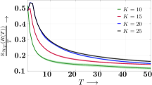
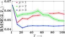
Regret analysis. First, we consider the case when estimates her followers’ preferences only on the basis of the feedback her stories receive from her followers. To that aim, we fix for all and , and simulate data from our feedback model of posting behavior for different number of topics . Then, we investigate the variation of the regret over time. Figure 1 summarizes the results which show that: (i) point estimates suffer linear regret whereas, posterior samples achieve logarithmic regret, thereby supporting our theoretical findings in Theorem 1 and Corollary 4; and, (ii) as the number of topics increases, the number of unknown preferences increases, and as a result, the regret increases.
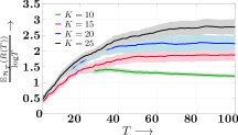
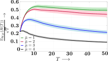
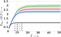
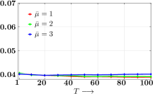
Next, we consider the case when additionally utilizes the feedback her followers give to others. To that aim, we set , sample and simulate our model on user for different value of . Figure 2 summarizes the results which show that: (i) the additional information (i.e., the feedback to others) significantly reduces the regret—even point estimates achieve a regret of , and moreover, posterior samples achieve a constant regret (i.e., ), thereby supporting Theorem 2 and Theorem 3; and, (ii) as increases, estimates their followers’ preferences on the basis of a larger amount of feedback and, as a result, the regret decreases.
Model estimation. To investigate the performance of our utility estimation framework, we first generate by simulating data from our model with and sample . Then, we train our model using the generated , for different and values using our two estimation methods from Section 4. Finally, we evaluate the accuracy of model estimation procedures in terms of root mean square error (RMSE) between the estimated and true parameters, i.e.,
Figure 3 summarizes the results the method based on linear loss minimization, which show that, (i) as increases and we feed more training samples into the estimation procedure, the accuracy increases; (ii) similarly, as increases and we feed more feedback into the estimation procedure, the accuracy increases; and, (iii) the estimation accuracy for posterior samples is significantly better than for point estimates;
6 Experiments on real data
In this section, we apply our utility estimation algorithms to several real datasets gathered from Twitter and Reddit and then, using the utility estimation framework described in Section 4, show that of the users in the Twitter datasets and of the users in the Reddit datasets use the feedback they receive from their followers to decide what to post next.
Data description and experimental setup. We collect Twitter and Reddit data for evaluating our utility estimation methods.
— Twitter: We used data gathered from Twitter as reported in previous work [14], which comprises the profiles of million users, billion directed follow links among them, and billion public tweets posted by these users, where the underlying link information is based on a snapshot taken at the time of data collection, in September 2009. Here, we focused on the tweets published during a two month period, from July 1, 2009 to September 26, 2009, which allows us to consider the set of followers of a user to be approximately static.
In our experiments, a follower provides feedback to a tweet published by a user if she retweets it333Since back in 2009, Twitter did not have a retweet button, we consider a Jaccard similarity between tokens contained in two tweets to decide if the latter is a retweet of former. and each topic corresponds to the most common444In case a tweet contains more than one hashtag, we consider the hashtag that is more common across our dataset. hashtag a tweet contains. Moreover, using manual inspection, we tracked down the hashtags used in three different themes to create three datasets:
-
—
Brazil: Brazil elections which took place in latter 2010, where , and .
-
—
TOT: Top US conservatives and liberals on Twitter, where , and .
-
—
Iran: Iran presidential elections in 2009, where , and .
In each of the above datasets, we filtered out hashtags that were used less than times and users who posted less than four tweets with at least two of these hashtags or whose tweets were not retweeted more than four times by at least 2 followers. Moreover, for each of user , we tracked down the five followers who retweeted her tweets more frequently and, for each these followers, we reconstructed the feedback they provided to her and others by collecting all their retweets as well as the tweets posted by all the users they follow.
— Reddit: We used publicly available data gathered from Reddit555https://archive.org/details/2015_reddit_comments_corpus, which comprises the profiles of million users and million comments posted by these users in the month of May, 2015. In our experiments, a user provides feedback to a message published by a user if she replied to it and each topic corresponds to the subreddit in which a comment was written. Here, we tracked down the subreddits in three different themes to create three datasets:
-
—
Leisure: r/funny, r/pics and r/WTF, where , and .
-
—
Sports: r/CFB, r/nba and r/nfl, where , and .
-
—
Learning: r/AdviceAnimals, r/TodayILearned, r/AskReddit and
r/worldnews, where , and .
In each of the above datasets, we only considered users who have made at least 20 top-level comments in at least 2 distinct categories . Moreover, for these users , we tracked down the five users who have replied to their comments more frequently and consider them to be the neighbors of . Finally, for each of these followers, we reconstructed the feedback they provided to and others by collecting all their replies as well as the comments posted by all their neighbors.
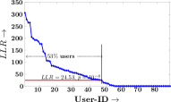
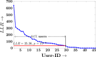
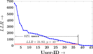
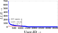
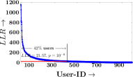
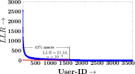
Results. We determined whether each user in each of the six datasets utilizes the feedback she receives from each of her followers to decide what to post next using the utility estimation framework described in Section 4. Figure 4 summarizes the results, which show that, at p-value , we can reject the hypothesis that users do not utilize the feedback they receive from their followers for %, %, % of the users in the Twitter datasets and for %, %, % of the users in the Reddit datasets.
7 Conclusions
In this paper, we introduced a feedback model of posting behavior in social media. The model allowed us: (i) to investigate under which conditions can a user succeed at maximizing the (positive) feedback she receives; and, (ii) to determine whether a user utilizes the feedback she receives from each of her followers to decide what to post next using observational data. Moreover, we performed experiments on synthetic and real data gathered from Twitter and Reddit to illustrate our theoretical findings, show that our estimation methods are able to accurately recover users’ underlying utility functions, and provide empirical evidence that of the users in the Twitter datasets and of the users in the Reddit datasets use the feedback they receive from their followers to decide what to post next.
There are many interesting venues for future work. For example, we have assumed that the followers’ preferences are not influenced by the users’ posting behavior. It would be interesting to analyze a scenario in which both users and the followers influence each other. We have considered a simple linear utility function, a natural next step would be considering more complex utility functions with higher predictive power. Finally, it would be very interesting to apply our utility estimation methods to real data from other social media platforms, e.g., Facebook.
References
- [1] Efforts to attract the youth vote continue as election day approaches. https://dailyiowan.com/2018/10/09/efforts-to-attract-the-youth-vote-continue-as-election-day-approaches/. Accessed: 2018-10-30.
- [2] What celebrities can teach companies about social media. https://www.wsj.com/articles/what-celebrities-can-teach-companies-about-social-media-1444788220. Accessed: 2018-10-30.
- [3] Why do some of your friends get more likes than others? https://www.huffingtonpost.com/simone-collins/why-do-some-of-your-friends-get-likes_b_6800102.html.
- [4] S. N. Afriat. The construction of utility functions from expenditure data. International economic review, 8(1):67–77, 1967.
- [5] S. Agrawal and N. Goyal. Further optimal regret bounds for thompson sampling. In Artificial Intelligence and Statistics, pages 99–107, 2013.
- [6] S. Agrawal and N. Goyal. Thompson sampling for contextual bandits with linear payoffs. In International Conference on Machine Learning, pages 127–135, 2013.
- [7] A. Aprem and V. Krishnamurthy. Utility change point detection in online social media: A revealed preference framework. IEEE Transactions on Signal Processing., 65(7):1869–1880, 2017.
- [8] P. Auer and R. Ortner. Logarithmic online regret bounds for undiscounted reinforcement learning. In Advances in Neural Information Processing Systems, pages 49–56, 2007.
- [9] M.-F. Balcan, A. Daniely, R. Mehta, R. Urner, and V. V. Vazirani. Learning economic parameters from revealed preferences. In International Conference on Web and Internet Economics, pages 338–353. Springer, 2014.
- [10] E. Beigman and R. Vohra. Learning from revealed preference. In Proceedings of the 7th ACM Conference on Electronic Commerce, pages 36–42. ACM, 2006.
- [11] M. Burke and R. Kraut. Using facebook after losing a job: Differential benefits of strong and weak ties. In Proceedings of the 2013 conference on Computer supported cooperative work, pages 1419–1430. ACM, 2013.
- [12] M. Burke and R. E. Kraut. Growing closer on facebook: changes in tie strength through social network site use. In Proceedings of the SIGCHI conference on human factors in computing systems, pages 4187–4196. ACM, 2014.
- [13] M. Burke, C. Marlow, and T. Lento. Social network activity and social well-being. In Proceedings of the SIGCHI conference on human factors in computing systems, pages 1909–1912. ACM, 2010.
- [14] M. Cha, H. Haddadi, F. Benevenuto, P. K. Gummadi, et al. Measuring user influence in twitter: The million follower fallacy. Icwsm, 10(10-17):30, 2010.
- [15] J. Cheng, C. Danescu-Niculescu-Mizil, and J. Leskovec. How community feedback shapes user behavior. arXiv preprint arXiv:1405.1429, 2014.
- [16] L. De Vries, S. Gensler, and P. S. Leeflang. Popularity of brand posts on brand fan pages: An investigation of the effects of social media marketing. Journal of interactive marketing, 26(2):83–91, 2012.
- [17] U. M. Dholakia, R. P. Bagozzi, and L. K. Pearo. A social influence model of consumer participation in network-and small-group-based virtual communities. International journal of research in marketing, 21(3):241–263, 2004.
- [18] F. Echenique, D. Golovin, and A. Wierman. A revealed preference approach to computational complexity in economics. In Proceedings of the 12th ACM conference on Electronic commerce, pages 101–110. ACM, 2011.
- [19] N. B. Ellison, J. Vitak, R. Gray, and C. Lampe. Cultivating social resources on social network sites: Facebook relationship maintenance behaviors and their role in social capital processes. Journal of Computer-Mediated Communication, 19(4):855–870, 2014.
- [20] R. Gray, N. B. Ellison, J. Vitak, and C. Lampe. Who wants to know?: question-asking and answering practices among facebook users. In Proceedings of the 2013 conference on Computer supported cooperative work, pages 1213–1224. ACM, 2013.
- [21] N. Grinberg, P. A. Dow, L. A. Adamic, and M. Naaman. Changes in engagement before and after posting to facebook. In Proceedings of the 2016 CHI Conference on Human Factors in Computing Systems, pages 564–574. ACM, 2016.
- [22] N. Grinberg, S. Kalyanaraman, L. A. Adamic, and M. Naaman. Understanding feedback expectations on facebook. In Proceedings of the 2017 ACM Conference on Computer Supported Cooperative Work and Social Computing, pages 726–739. ACM, 2017.
- [23] T. Jaksch, R. Ortner, and P. Auer. Near-optimal regret bounds for reinforcement learning. Journal of Machine Learning Research, 11(Apr):1563–1600, 2010.
- [24] A. N. Joinson. Looking at, looking up or keeping up with people?: motives and use of facebook. In Proceedings of the SIGCHI conference on Human Factors in Computing Systems, pages 1027–1036. ACM, 2008.
- [25] M. Karimi, E. Tavakoli, M. Farajtabar, L. Song, and M. Gomez-Rodriguez. Smart Broadcasting: Do you want to be seen? In KDD ’16: Proceedings of the 22nd ACM SIGKDD International Conference on Knowledge Discovery in Data Mining, 2016.
- [26] A. Y. Koo. An empirical test of revealed preference theory. Econometrica: Journal of the Econometric Society, pages 646–664, 1963.
- [27] A. Mas-Colell. The recoverability of consumers’ preferences from market demand behavior. Econometrica: Journal of the Econometric Society, pages 1409–1430, 1977.
- [28] A. Ostrowski. Integral inequalities. In Functional Equations and Inequalities, pages 387–419. Springer, 2010.
- [29] P. A. Samuelson. Consumption theory in terms of revealed preference. Economica, 15(60):243–253, 1948.
- [30] N. Spasojevic, Z. Li, A. Rao, and P. Bhattacharyya. When-to-post on social networks. In Proceedings of the 21th ACM SIGKDD International Conference on Knowledge Discovery and Data Mining, 2015.
- [31] S. S. Wilks. The large-sample distribution of the likelihood ratio for testing composite hypotheses. The Annals of Mathematical Statistics, 9(1):60–62, 1938.
- [32] M. Zadimoghaddam and A. Roth. Efficiently learning from revealed preference. In International Workshop on Internet and Network Economics, pages 114–127. Springer, 2012.
- [33] A. Zarezade, A. De, U. Upadhyay, H. R. Rabiee, and M. Gomez-Rodriguez. Steering social activity: A stochastic optimal control point of view. Journal of Machine Learning Research, 18:205–1, 2017.
- [34] A. Zarezade, U. Upadhyay, H. Rabiee, and M. Gomez-Rodriguez. Redqueen: An online algorithm for smart broadcasting in social networks. In WSDM ’17: Proceedings of the 10th ACM International Conference on Web Search and Data Mining, 2017.
8 Appendix
8.1 Proof of Theorem 1
Consider a special case, where the number of topics is ; has only one follower with ; the weights ; the user preferences ; and the prior parameters . Then, the regret is
Since, , we have , where is the number of stories about topic . Now, makes the initial estimates , and therefore, a topic is chosen randomly. Let us assume that topic (the wrong category with minimum utility) is selected and a story from that topic is shared. If likes this story, which can happen with probability , then and topic is again selected at next time . At , again increases (decreases) with probability . Note that, keeps choosing topic as long as i.e. , and the possibility of selecting topic only arises when . Such a situation can be mapped to an instance of a simple one dimensional random walk, where the walker starts from origin at , if a story from topic is shared. The walker moves to right (left) if user does (not) like the story. Now, the expected time of the first return to origin in a simple random walk is infinite. Therefore, once starts posting the messages with category , the expected time that for the first time [feller1968introduction]. Therefore, . More formally, we have:
| (14) |
Now, in the random walk setting, is the amount of time the walker stays on the positive or right side of the line, and therefore, greater than the time of first return to origin, which is infinite. Therefore, the walker stays on the right side for the entire , given the first step is taken towards the right side is . Hence, we have . hence .
8.2 Proofs of Theorems 2 and 3
Preliminaries. To prove these theorems, we first present few notations which will be used throughout both the proofs.
For the sake of brevity, we define (i) ;
(ii) for all ;
(iii) ; (iv) as the number of posts made by broadcaster up to and including time , that have category ;
(iv) ;
(v) as the number of messages with category , which may observe as they are appearing the wall of until and excluding time ;
(vi) as the c.d.f of Beta distribution with parameters and ;
(vii) as the c.d.f in Binomial distribution with parameters ;
(viii) as the probability mass function in Binomial distribution function;
(ix) ;
(x) ;
(xi) ;
(xii) ;
(xiii) ; and
(xiv) , where .
Furthermore, we define
| (15) |
Equality is due to definitions (ii) and (iii) .
| (16) |
Proof of Theorem 2. We have,
| (17) |
The inequality is obtained using (i) the triangle inequality of max norm; (ii) the fact that ; and (iii) , where (iii) reduces the summation over to . Since, , we have
| (18) |
can be written as,
On expanding, we have to be same as
| (19) |
where and . Finally we observe that, . Hence,
| (20) |
From Eq. 18, we now have,
| (21) |
Then we apply Lemma 6 to obtain the required bound.
Proof of Theorem 3. To prove this theorem, we leverage the proof techniques of Agarwal et al in [5]. Without loss of generality, we assume that the set of categories ; is the optimum true category with maximum utility. We also denote denotes the time step at which a message with optimal category (i.e., category ) is posted for the -th time. In this context, we denote,
| (22) |
Then, we define two numbers so that,
| (23) |
where is set of positive rational numbers. Note that for both , . We define as the event that , and as the event that . Note that, since , So, we have . Hence, we can define
| (24) |
To prove the theorem, in the first step, we show that the regret is proportional to the sum of number of times a suboptimal category is posted. Then we decompose this quantity into three suitable quantities and provide individual bounds and then combine them. From, definition (xi), we note that . Therefore, the expected regret is proportional to the number of times a suboptimal category is posted.
| (25) |
where we recall that is the number of times a message with category has been posted up to and including time . So, . Therefore, we have,
| (26) |
Now, we are going to bound these three sums individually.
— Bounding :
Inequality comes from Lemma 7. Inequality comes from the fact that and in the corresponding expression, the expectation is taken over all sources of randomness. Since, denotes the time step at which a message with optimal category (i.e. ) is posted for the -th time, at times other than , the indicator term becomes zero, which explains the last inequality . From Lemma 8, we note that is
| (27) |
which is .
Next we give bound of the second term in Eq. 26.
— Bounding .
We observe that,
| (28) |
Inequality is due to the following. If for all , then . Inequality is due to the fact that cdf of Beta() is decreasing w.r.t. and increasing w.r.t [5]. Inequality is due to the relation between Beta distribution with integer parameters and Binomial distributions [5, Fact 3, Appendix A]. Inequality is due to Chernoff-Holding bound [5, Fact 1, Appendix A]. Then, from Eq. 28, we obtain that,
| (29) |
Now, we split . For time such that , we use the definition of from Eq. 24 to have,
Now consider that is the largest time until . Then we have,
Then we have, has order
| (30) |
where, .
— Bounding .
We define is the time at which category is posted time. Then, we observe that
| (31) |
Inequality holds because the indicator is only activated when category posted. Inequality is due to an union bound and inequality is due to Chernoff-Hoeffding bounds [5, Fact 1, Appendix A]. Combining Eq. 27, 30, 31, we obtain the required bound.
8.3 Auxilliary lemmas
Lemma 5.
If the rate of messages in ’s feed are exposed to with Poisson distribution having rate for each category , and are total number of such messages for category , observed until timestep , then we have
| (32) |
Proof: can be written as,
| (33) | |||
| (34) |
— Case . In this case, is increasing and is decreasing. So we apply Chebyschev inequality [28] to have
0.4
which provides the required expression.
— Case . Since , implies . Hence, the required integral is less than
Lemma 6.
If and have the similar meanings as the previous lemma, then we have
| (35) |
Proof: For , we have
which gives the required bound. For , we have
Lemma 7.
[5] If we define , then
Lemma 8.
If denote the time step at which the optimal category is selected for the -th time. Then,
where, , , ; . Note that from Eq. 23, .
Proof.
We leverage the proof of [5, Lemma 4] to prove this lemma Let , .
| (36) |
Inequality is because for all implies
Inequality is due to the fact that is increasing in and decreasing in , and we choose . Equality holds due to for simple mapping from Beta distribution to Binomial distribution when the parameters for Beta distribution are integers. Then, we have:
| (37) |
We denote , and observe that . This is because, for . We express as the sum of two terms , where . We note that,
| (38) |
Inequality is due the fact that
Inequality is obtained by leveraging the proof of Lemma 4 in Agarwal et al in [5]. Now we bound . Using the proof of Lemma 4 in Agarwal et al in [5], we have, for . Then, we have
| (39) |
Adding, Eq. 38 and 39, and then substituting back to Eq. 37, we observe that, equals to
The last inequality follows by taking only the dominating term.
∎