Eternal Inflation in Swampy Landscapes

Abstract

The much discussed swampland conjectures suggest significant constraints on the properties of string theory landscape and on the nature of the multiverse that this landscape can support. The conjectures are especially constraining for models of inflation; in particular, they exclude the existence of de Sitter (dS) vacua. If the conjectures are false and dS vacua do exist, it still appears that their construction in string theory requires a fair amount of fine-tuning, so they may be vastly outnumbered by AdS vacua. Here we explore the multiverse structure suggested by these considerations. We consider two scenarios: (i) a landscape where dS vacua are rare and (ii) a landscape where dS vacua do not exist and the dS potential maxima and saddle points are not flat enough to allow for the usual hilltop inflation, even though slow roll inflation is possible on the slopes of the potential. We argue that in both scenarios inflation is eternal and all parts of the landscape that can support inflation get represented in the multiverse. The spacetime structure of the multiverse in such models is nontrivial and is rather different from the standard picture.

I Introduction

String theory predicts the existence of a vast landscape of vacuum states with diverse properties Bousso and Polchinski (2000); Susskind (2003); Douglas (2003); Kachru et al. (2003); Denef and Douglas (2004); Douglas and Kachru (2007). In the cosmological context this suggests the picture of an eternally inflating multiverse, where different spacetime regions are occupied by different vacua. Inflation is driven by metastable positive-energy vacua and transitions between the vacua occur through quantum tunneling, with bubbles of daughter vacuum nucleating and expanding in the parent vacuum background. According to this picture, our local region originated as a result of tunneling from some inflating parent vacuum and then went through a period of slow-roll inflation. An alternative version of the multiverse scenario is based on the picture of quantum diffusion near local maxima or saddle points of the potential Vilenkin (1983a); Starobinsky (1986); Linde (1992). The multiverse cosmology provides a natural stage for anthropic selection; in particular, it gives a natural explanation to the fine-tuning necessary for inflaton potentials and for the smallness of the dark energy density.

The multiverse picture, however, is now being seriously questioned. Inflation is typically described by a quantum scalar field $\phi$ (the inflaton) coupled to gravity. The character of inflation, its predictions, and its very existence depend on the form of the inflaton potential $V(\phi)$. Considering the vastness of the landscape, one might expect that it includes nearly all imaginable forms of $V(\phi)$. However, there is growing evidence that a wide class of quantum field theories do not admit a UV completion within the theory of quantum gravity, even though they look perfectly consistent otherwise. Such theories are said to belong to the swampland, as opposed to the landscape. A number of different criteria that the landscape potential $V(\phi)$ should satisfy have recently been conjectured. One such criterion, proposed in Obied et al. (2018), requires that

$$|\nabla V|>c~{}V,$$ (1)

where $c={\cal O}(1)$. As it stands, however, this requirement is too restrictive. Not only it excludes metastable, and even unstable, de Sitter (dS) vacua, but it is also in considerable tension with slow-roll inflation Agrawal et al. (2018); Achucarro and Palma (2019); Kehagias and Riotto (2018); Kinney et al. (2019); Garg and Krishnan (2018); Dias et al. (2019); Das (2019) and even with the Standard Model of particle physics Denef et al. (2018); Choi et al. (2018); Murayama et al. (2018). We now know that the conjecture (1) is actually false: a number of counterexamples in models of string theory compactification have been presented in Refs. Conlon (2018); Blanco-Pillado et al. (2019a); Olguin-Trejo et al. (2019).

A modified, or ‘refined’ swampland conjecture has been proposed in Refs. Ooguri et al. (2019); Garg and Krishnan (2018); Garg et al. (2019); Andriot (2018). It asserts that

$$|\nabla V|>c~{}V~{}~{}~{}~{}{\rm or}~{}~{}~{}~{}{\rm min}~{}V^{\prime\prime}<-c^{\prime}~{}V,$$ (2)

where ${\rm min}~{}V^{\prime\prime}$ is the smallest Hessian eigenvalue and $c,c^{\prime}$ are positive constants ${\cal O}(1)$.

Inflationary cosmology has impressive observational support, and at this time there seem to be no viable alternatives. It seems reasonable therefore to assume that the swampland criteria, whatever their final form will be, must be consistent with slow-roll inflation. It is possible for example that the constants $c,c^{\prime}$ in Eq. (2) have somewhat smaller values, e.g., $\sim 0.1-0.01$ Kinney et al. (2019). This would be compatible with slow-roll inflation, even though the possible form of the inflaton potential would be strongly restricted. (See Motaharfar et al. (2019); Ashoorioon (2019); Heckman et al. (2019) for other suggestions to avoid the swampland restrictions in inflation.) Depending on the values of $c$ and $c^{\prime}$, quantum diffusion of the inflaton field and the associated eternal inflation may or may not be excluded Matsui and Takahashi (2019); Dimopoulos (2018); Kinney (2019); Brahma and Shandera (2019); Wang et al. (2019). Some authors have even suggested that eternal inflation may be forbidden by some fundamental principle Dvali and Gomez (2019); Dvali et al. (2019); Rudelius (2020).

It is of course possible that the swampland conjecture (2) is false and the landscape does include some dS vacua Kallosh et al. (2019); Akrami et al. (2019). But even then it seems that the construction of such vacua in string theory is not straightforward and may require a fair amount of fine-tuning. This suggests that the number of dS vacua in the landscape may be much smaller than that of AdS vacua.

In the present paper we shall explore the multiverse structure suggested by these considerations. In the next section we assume that the swampland conjecture is false and dS vacua do exist, but they are vastly outnumbered by AdS (and Minkowski) vacua. We find that the transition rates between dS vacua in this case are very strongly suppressed and the spacetime structure of the multiverse is rather different from what is usually assumed. We discuss under what conditions the successful prediction of the observed cosmological constant still holds and find that these conditions are relatively mild.

In Section III we shall assume that something like the refined swampland conjecture is true, so that dS vacua do not exist and dS maxima and saddle points are not flat enough to allow for hilltop inflation (but slow-roll inflation is possible on the slopes, away from the hilltops). We shall argue however that eternal inflation would still occur. It would be driven by

inflating bubble walls, while slow roll inflation would take place on the slopes of the potential. The multiverse in this scenario would also have a rather nontrivial spacetime structure.

II Landscape dominated by AdS vacua

II.1 Transition rates

We shall first assume that dS vacua do exist, but they are vastly outnumbered by AdS vacua. Note that this does not necessarily mean that the distances between dS vacua in the field space are much larger than those between AdS vacua. If ${\cal N}$ is the total number of vacua (of a given kind), $l$ is the typical distance between them and $D$ is the dimensionality of the landscape, we can write

$$r\equiv\frac{{\cal N}_{dS}}{{\cal N}_{AdS}}\sim\left(\frac{l_{AdS}}{l_{dS}}\right)^{D}.$$ (3)

With $D\gtrsim 100$, we can have $r\ll 1$ even if $l_{dS}$ is only larger than $l_{AdS}$ by a factor ${\cal O}(1)$.

II.1.1 Tunneling transitions

Consider now quantum decay of a metastable dS vacuum. We shall adopt a naive picture where the string landscape is locally represented by a random Gaussian field $U(\phi)$ characterized by an average value ${\bar{U}}$, a typical amplitude $U_{0}$ and a correlation length $\xi$ in field space. A simple analytic estimate of the tunneling action was given by Dine and Paban Dine and Paban (2015). They assumed that the vacuum decay rate is controlled mainly by the quadratic and cubic terms in the expansion of $U(\phi)$ about the potential minimum. Then the tunneling action can be estimated as

$$S\sim C\frac{m^{2}}{\gamma^{2}},$$ (4)

where $m^{2}$ is an eigenvalue of the Hessian matrix at the minimum, $\gamma\sim U_{0}/\xi^{3}$ is the typical coefficient of a cubic expansion term and $C\sim 50$ is a numerical coefficient. A typical Hessian eigenvalue is $m^{2}\sim U_{0}/\xi^{2}$, which gives

$$S\sim C\frac{\xi^{4}}{U_{0}}.$$ (5)

For a weakly coupled theory we have $U_{0}/\xi^{4}\ll 1$, so $S\gg 100$. In particular, we expect this to be the case for an axionic landscape, where the potential is induced by instantons.

In a $D$-dimensional landscape one can expect to have $\sim D$ decay channels out of any dS vacuum. The highest decay rate corresponds to one of the smallest Hessian eigenvalues, which have been estimated in Yamada and Vilenkin (2018) as

$$m_{min}^{2}\sim\frac{U_{0}}{\sqrt{D}\xi^{2}}.$$ (6)

This gives

$$S_{min}\sim\frac{C}{\sqrt{D}}\frac{\xi^{4}}{U_{0}}.$$ (7)

Since the vacua surrounding a given dS vacuum are mostly AdS, this dominant decay channel will typically lead to an AdS vacuum. The tunneling action to a dS vacuum will typically be greater by a factor $\sim\sqrt{D}\gg 1$. Transitions to dS vacua will therefore be strongly suppressed.

II.1.2 Non-tunneling transitions

The above discussion assumes that quantum tunneling between dS vacua is possible. However, if the density of dS vacua is very low, most of them may be completely surrounded by AdS vacua, and Coleman-DeLuccia (CdL) instantons connecting such vacua may not exist. Some rare dS vacua would have other dS vacua in their vicinity and would form eternally inflating islands Clifton et al. (2007), but still there would be no tunneling between the islands. However, Brown and Dahlen (BD) have emphasized in Ref. Brown and Dahlen (2011) that quantum transitions between vacua can occur even in the absence of instantons. These non-tunneling transitions may require rather unlikely quantum fluctuations, which are far more improbable than the fluctuations needed for the tunneling transitions. The rate of such transitions is therefore likely to be highly suppressed compared to the tunneling transitions. BD have argued that with non-tunneling transitions included, any landscape would become irreducible – that is, it would be possible to reach any vacuum in the landscape from any other vacuum by a finite sequence of quantum transitions.

As an example of a non-tunneling transition, BD suggested that the scalar field $\phi$ in some dS vacuum of an island could develop a large velocity $({\dot{\phi}})$ fluctuation in a finite region. The field could then ”fly over” the neighboring AdS vacua of the landscape, ending up in some distant dS vacuum of another island. If the new dS region is bigger than the corresponding horizon, it would inflate without bound.

We studied the dynamics of such flyover transitions in Ref. Blanco-Pillado et al. (2019b) in models where competing tunneling transitions are also possible. We found that in most cases tunnelings and flyovers have a comparable rate, but in the case of upward transitions from dS vacua the rate of flyovers can be significantly higher. The same method can be applied to estimate the flyover rate in cases where tunneling is impossible. Following Blanco-Pillado et al. (2019b), we shall assume that the initial fluctuation leaves the scalar field and the spatial metric homogeneous, while the time derivative of the field acquires a large value in a roughly spherical region. Time derivatives of the metric also get modified in that region, as required by the Hamiltonian and momentum constraints. Once the fluctuation occurred, the subsequent evolution is assumed to follow the classical equations of motion.

The required magnitude of the field velocity fluctuation in a region of size $l$ can be estimated as

$${\dot{\phi}}_{l}^{2}=2C\Delta V,$$ (8)

where $\Delta V$ is the maximal potential difference that the field has to overcome on the way from parent to daughter vacuum and $C>1$ is a numerical coefficient accounting for the Hubble friction. Since the fluctuation occurs with $\phi$ at its parent vacuum value $\phi_{p}$, the field $\phi$ can be approximated by a free scalar field of mass $m^{2}=V^{\prime\prime}(\phi_{p})$. In the absence of fine-tuning we expect $m\gtrsim H_{p}$, where $H_{p}\sim V_{p}^{1/2}$ is the expansion rate in the parent vacuum. The rate of flyover transitions can then be estimated as

$$\kappa_{\rm flyover}\sim\exp\left(-\frac{{\dot{\phi}}_{l}^{2}}{2\langle{\dot{\phi}}^{2}\rangle_{l}}\right),$$ (9)

where $\langle X\rangle_{l}$ indicates vacuum expectation value of the operator $X$ averaged over the length scale $l$. The variance $\langle{\dot{\phi}}^{2}\rangle_{l}$ for a free massive field in de Sitter space with $H\lesssim m$ was calculated in Ref. Blanco-Pillado et al. (2019b). It is

$$\langle{\dot{\phi}}^{2}\rangle_{l}\sim 10^{-2}ml^{-3}$$ (10)

for $ml\gtrsim 1$ and

$$\langle{\dot{\phi}}^{2}\rangle_{l}\sim 10^{-2}l^{-4}$$ (11)

for $ml\lesssim 1$. The fluctuation length scale $l$ should be set as the smallest scale that can yield a new inflating vacuum region.

The length scale $l$ and the factor $C$ in (8) generally depend on the shape of the potential between the parent and daughter vacua, but the estimate can be made more specific in some special cases. One example is when $\Delta V\sim V_{p}$. In this case the flyover time is

$$\Delta t\sim\frac{\Delta\phi}{\sqrt{C\Delta V}}\lesssim\frac{1}{\sqrt{\Delta V}}\sim\frac{1}{H},$$ (12)

where $H$ is the average Hubble expansion rate during the flyover, $\Delta\phi$ is the distance between the two vacua in the field space, and we assumed $\Delta\phi\lesssim 1$ in the second step. The inequality $H\Delta t\lesssim 1$ implies that the Hubble friction is not very significant and thus $C\sim 1$. It also indicates that the size of the fluctuation region does not change much in the course of the flyover.

We now have to consider two possibilities. If the energy density of the daughter vacuum is comparable to that of the parent vacuum, $V_{d}\sim V_{p}$, then in order to produce an inflating region of daughter vacuum, the scale $l$ should be comparable to the daughter vacuum horizon, $l\sim H_{d}^{-1}\sim H_{p}^{-1}$. Hence we obtain the following estimate for the transition rate,

$$\kappa_{\rm flyover}\sim\exp\left(-10^{2}m^{-1}H_{d}^{-1}\right),$$ (13)

where we have used $H_{d}^{2}\sim V_{d}$.

Alternatively, if $V_{d}\ll V_{p}$, the field $\phi$ arrives to the daughter vacuum value with a large velocity, ${\dot{\phi}}^{2}\sim V_{p}\gg V_{d}$, which has to be red-shifted before the vacuum dominated evolution can begin. During this transient period the field oscillates about the daughter vacuum value and the effective equation of state is that of a matter dominated universe, so the energy density evolves as $\rho\propto a^{-3}$. As $\rho$ decreases from $\sim V_{p}$ to $\sim V_{d}$, the fluctuation region expands by a factor of $(V_{p}/V_{d})^{1/3}$. By this time the size of the fluctuation region should be $\sim H_{d}^{-1}$, so its initial size has to be $l\sim(H_{p}^{2}H_{d})^{-1/3}$. This yields the same estimate for the transition rate as in Eq. (13). This estimate suggests that, unlike the CdL tunneling, flyover transitions to low-energy vacua are typically much stronger suppressed than transitions with $V_{d}\sim V_{p}$. The reason is that such transitions require a fluctuation in a much larger region.

For $\Delta V\gg V_{p}$, the energy density in the fluctuation region would be much higher than in the parent vacuum, so the initial fluctuation would be affected by large gravitational back-reaction and the field $\phi$ cannot be approximated as a free field in dS space. We made no attempt to estimate the transition rate in this case. On general grounds, one can expect that the rate should obey the lower bound

$$\kappa\gtrsim e^{-S_{p}},$$ (14)

where $S_{p}=\pi/H_{p}^{2}$ is the de Sitter entropy of the parent vacuum. The idea is that the transition in a horizon-size region should occur at least once per de Sitter recurrence time, $\tau_{rec}\sim e^{-S_{p}}$. Comparing the exponent $S_{p}$ with the typical downward transition action (5), we find

$$\frac{S_{p}}{S_{\downarrow}}\sim\frac{U_{0}}{H_{p}^{2}}\frac{1}{\xi^{4}}\sim\frac{1}{\xi^{4}}.$$ (15)

This ratio is large if the correlation length $\xi$ is sub-Planckian.

We note that for some values of the parameters in the regime where $\Delta V\sim V_{p}\gg V_{d}$ our estimate (13) can violate the bound (14). This is not necessarily a problem, since in this regime the fluctuation has to occur on a scale much greater than the parent horizon, and it is not clear that its timescale should be bounded by one horizon region’s recurrence time. Assuming that dS entropy is additive on super-horizon scales, the entropy of a region of size $l\sim(H_{p}^{2}H_{d})^{-1/3}$ is $S_{l}\sim(lH_{p})^{3}S_{p}\sim(H_{p}H_{d})^{-1}$. Then the bound $\kappa\gtrsim\exp(-S_{l})$ is satisfied for $m\gtrsim H_{p}$.

II.2 Spacetime structure

We now consider the spacetime structure of the multiverse in this kind of model. We assume that for most pairs of dS vacua the paths connecting them in the field space will pass through some AdS or Minkowski vacua. A simple example of this sort is illustrated in Fig. 1, where two dS vacua $X$ and $Y$ are separated by a Minkowski vacuum $Z$ in a $1D$ landscape. If a field velocity fluctuation from vacuum $X$ creates a spherical region of vacuum $Y$, this region has to be separated from the parent vacuum by a shell-like region of vacuum $Z$. The boundaries of this Minkowski shell accelerate into both $X$ and $Y$ regions. For an observer in the parent vacuum $X$, the transition $X\to Y$ looks like nucleation of a Minkowski bubble of vacuum $Z$. An observer inside that bubble will see the dS region of vacuum $Y$ collapse to a black hole. The black hole mass can be estimated as

$$M\sim V_{d}H_{d}^{-3}\sim H_{d}^{-1}.$$ (16)

This black hole contains the new dS region inflating like a balloon. A Penrose diagram for this spacetime structure is shown in Fig. 2. It is similar to that for a false vacuum bubble nucleated during inflation, as discussed in Ref. Deng et al. (2017). Note that this spacetime structure is expected for both $V_{p}>V_{d}$ and $V_{p}<V_{d}$.

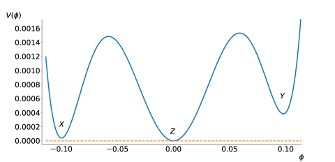
Figure 1: A $1D$ landscape with two dS vacua separated by a Minkowski

vacuum.

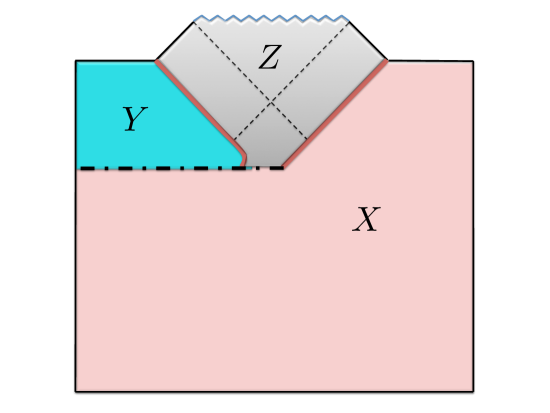
Figure 2: Causal diagram for a transition $X\to Y$ in the landscape of Fig. 1. The inflating bubble of $Y$ vacuum is contained in a black hole, which is formed inside an expanding Minkowski bubble of $Z$ vacuum.

To verify this picture, we performed numerical simulations of an upward flyover transition $X\to Y$ in the landscape of Fig. 1. At the initial moment $t_{0}$ we set $\phi=\phi_{p}$ and ${\dot{\phi}}={\dot{\phi}}_{0}f(r)$, where $r$ is a radial coordinate, $f(r)=\exp(-r^{2}/2l^{2})$ and $l\sim H_{d}^{-1}$. A general spherically symmetric metric can be brought to the form

$$ds^{2}=-dt^{2}+B^{2}dr^{2}+R^{2}d\Omega^{2},$$ (17)

where $d\Omega^{2}$ is the metric on a unit sphere and $B$ and $R$ are functions of $t$ and $r$. At $t=t_{0}$ we set $B=1$ and $R=r$, so the spatial metric is flat. The time derivatives of $B$ and $R$ at $t_{0}$ can be determined from the constraint equations. We then evolved these initial conditions using the code we developed in Refs. Deng et al. (2017); Blanco-Pillado et al. (2019b). The scalar field potential we use is (Fig. 1)

$$V(\phi)=\phi^{2}[(10\phi-1)^{2}+0.1\phi][(10\phi+1)^{2}-0.01\phi].$$ (18)

We performed the simulation for different values of the parameter ${\dot{\phi}}_{0}$. With $l=2H^{-1}_{d}$, the minimal value that yielded a new inflating region corresponds to $C\approx 5$ in Eq. (8). The field evolution $\phi(r,t)$ is shown in Fig. 3. By the end of the simulation we have well defined regions of $Y$ and $Z$ vacua bounded by bubble walls. The radius $r$ is a ”comoving” coordinate, so the radius of the inflating region remains nearly constant. But the physical radius of this region grows with time. We have also verified the formation of black hole apparent horizons (See Fig. 3). The resulting black hole masses in our simulations agree with the estimate (16) (within a factor of a few) for $M$ in the range $\mathcal{O}(1)$-$\mathcal{O}(100)$ in Planck units. If $Z$ is an AdS vacuum, the interior of the AdS region eventually undergoes a big crunch. As viewed from the parent vacuum $X$, the transition process looks like nucleation of a bubble of AdS or Minkowski vacuum $Z$. In either case the new inflating region gets completely separated from the parent vacuum.

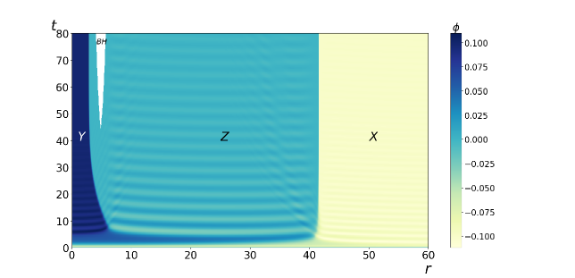
Figure 3: Field evolution in a $1D$ landscape with two dS vacua separated by a Minkowski vacuum (Fig. 1). Initially the field is in the parent vacuum $X$. A field velocity fluctuation creates a spherical region of vacuum $Y$, which is separated from the parent vacuum by a shell-like region of vacuum $Z$. Oscilations of $\phi$ about the minimum $\phi=0$ are clearly visible in that region. Formation of a black hole is signaled by the appearance of apparent horizons. The white area in the diagram corresponds to the spacetime region between the inner and outer apparent horizons.

II.3 Volume fractions

Observational predictions in multiverse models depend on one’s choice of the probability measure. Different measure prescriptions can give vastly different answers. (For a review of this ‘measure problem’ see, e.g., Freivogel (2011).) However, measures that are free from obvious pathologies tend to yield similar predictions. For definiteness we shall adopt the scale-factor cutoff measure which belongs to this class Linde and Mezhlumian (1993); Linde et al. (1994); De Simone et al. (2008); Bousso et al. (2009). The probability of observing a region of type $i$ can then be roughly estimated as

$$P_{i}\sim P_{i}^{(prior)}n_{i}^{(obs)},$$ (19)

where the ”prior” probability is

$$P_{i}^{(prior)}\propto\kappa_{ij}f_{j},$$ (20)

$\kappa_{ij}$ is the transition rate to $i$ from inflating parent vacuum $j$, and $f_{j}$ is the volume fraction occupied by vacuum $j$ on a surface of constant scale factor $a$ in the limit of $a\to\infty$. The ”anthropic factor” $n^{(obs)}_{i}$ in (19) is the number of observers per unit volume in this type of region.

To characterize a multiverse with ${\cal N}_{dS}\ll{\cal N}_{AdS}$, let us first review the standard multiverse picture which assumes (implicitly) that these numbers are not vastly different Schwartz-Perlov and Vilenkin (2006). According to this picture, most of the inflating volume in the multiverse is occupied by the dominant vacuum, which has the slowest decay rate. This dominant vacuum typically has a very low energy density. Upward transitions (that is, transitions to higher-energy vacua) from the dominant vacuum and subsequent downward transitions populate other dS vacuum states. Such upward transitions have a very strongly suppressed rate, with a suppression factor $\sim\exp(-S_{D})$, where $S_{D}$ is the entropy of the dominant vacuum. However, since the path to any dS vacuum includes such an upward transition, the volume fractions of all relevant dS vacua include this suppression factor. One expects therefore that the relative volume fractions are typically of the order

$$\left|\ln(f_{i}/f_{j})\right|\sim\left|\ln\kappa_{\downarrow}\right|,$$ (21)

where $\kappa_{\downarrow}\sim e^{-S}$ with $S$ from Eq. (5) is a typical rate of downward transitions in the landscape. The ratio of the transition rates $\kappa_{ij}$ is typically of the same order (on a logarithmic scale). Hence we expect the prior probabilities $P_{i}^{(prior)}$ to vary by factors $\sim\kappa_{\downarrow}$.

Let us now discuss how this multiverse picture is modified in a landscape dominated by AdS vacua. We now have small groups of dS vacua with transitions between the groups strongly suppressed. Let us first see for a moment what would happen if the transitions between the groups were strictly impossible. The volume occupied by the vacua of the $j$-th group on a constant scale factor hypersurface, $a={\rm const}$, would then grow as De Simone et al. (2008)

$$V_{j}\propto e^{(3-q_{j})t},$$ (22)

where $t=\ln a$ is the scale-factor time. The parameter $q_{j}$ depends on the transition rates between the vacua of the island and between these vacua and the surrounding AdS vacua. As a rule of thumb, the value of $q_{j}$ is controlled mainly by the decay rate $\kappa_{j}^{(min)}$ (per Hubble volume per Hubble time) of the slowest decaying vacuum in the group, $q_{j}\approx\kappa_{j}^{(min)}$. In the limit of $t\to\infty$, the volume distribution would be dominated, by an arbitrarily large factor, by the group with the smallest value of $q_{j}$. Since the dominant group includes only a few dS vacua, it is highly unlikely to include a vacuum with a small enough cosmological constant to allow for galaxy formation. This situation would be disastrous for anthropic predictions of the multiverse models.

To understand the effect of very small transition amplitudes between the dS vacuum groups, let us consider a toy model described by the schematic

$$A\leftarrow X\leftrightarrow Y\rightarrow B.$$ (23)

Here, $A$ and $B$ are terminal (AdS or Minkowski) vacua, $X$ and $Y$ are dS vacua, and we assume that the transition rates between the vacua satisfy

$$\kappa_{XY},\kappa_{YX}\ll\kappa_{AX},\kappa_{BY}.$$ (24)

The volume fractions $f_{j}$ occupied by dS vacua $X$ and $Y$ satisfy the rate equations

$$\frac{df_{X}}{dt}=-(\kappa_{AX}+\kappa_{YX})f_{X}+\kappa_{XY}f_{Y},$$ (25)

$$\frac{df_{Y}}{dt}=-(\kappa_{BY}+\kappa_{XY})f_{Y}+\kappa_{YX}f_{X}.$$ (26)

If we neglect the dS transition rates $\kappa_{XY}$ and $\kappa_{YX}$, the solution is

$$f_{X}\propto\exp(-\kappa_{AX}t),~{}~{}~{}~{}f_{Y}\propto\exp(-\kappa_{BY}t).$$ (27)

Assuming for definiteness that $\kappa_{AX}<\kappa_{BY}$, $f_{X}$ decreases slower than $f_{Y}$ and dominates over $f_{Y}$ by an arbitrarily large factor in the limit of large $t$.

With the dS transitions included, the asymptotic solution of the rate equations at large $t$ has the form $f_{X},f_{Y}\propto e^{-qt}$, where $q>0$ is the smallest (by magnitude) eigenvalue of the transition matrix. The general solution of Eqs. (25),(26) is discussed in detail in Ref. Garriga et al. (2006). Here we are only interested in the limit (24). Assuming again that $\kappa_{AX}<\kappa_{BY}$, we find

$$q\approx\kappa_{AX},~{}~{}~{}~{}\frac{f_{Y}}{f_{X}}\approx\frac{\kappa_{YX}}{\kappa_{BY}-\kappa_{AX}}.$$ (28)

This solution can be understood as follows. The dS vacuum $X$ decays slower than vacuum $Y$; hence it dominates the volume and to the leading order its volume fraction $f_{X}$ can be approximated by Eq. (27). The vacuum $Y$ is populated by transitions from $X$ with a strongly suppressed rate $\kappa_{YX}$.

The vacua $X$ and $Y$ in this simple model can be thought of as representing different inflating islands. Eq. (28) then suggests that volume fractions of the islands vary by factors $\sim\kappa$, where $\kappa$ is the (strongly suppressed) transition rate between the islands.

II.4 Prediction for $\Lambda$

The probability distribution for the observed values of the cosmological constant can be represented as

$$P(\Lambda)\propto P_{prior}(\Lambda)n_{obs}(\Lambda).$$ (29)

In the early literature on this subject it seemed reasonable to assume that the prior distribution in the narrow range $\Delta\Lambda$,

$$|\Lambda|\lesssim 10^{-116},$$ (30)

where the density of observers is non-negligible, can be well approximated as

$$P_{prior}(\Lambda)\approx{\rm const}.$$ (31)

The reason is that the natural range of the distribution is $|\Lambda|\lesssim 1$ and, as the argument goes, any smooth distribution will look flat in a tiny fraction of its range. The anthropic factor $n_{obs}(\Lambda)$ is usually assumed to be proportional to the fraction of matter clustered into large galaxies. The resulting prediction for $\Lambda$ is in a good agreement with the observed value $\Lambda_{0}\sim 10^{-118}$.

It was however argued in Ref. Schwartz-Perlov and Vilenkin (2006) that the assumption of a flat prior (31) may not be justified in the string landscape. Vacua with close values of $\Lambda$ are not necessarily very close in the landscape and may have vastly different prior probabilities. In models of the kind we are discussing here these probabilities can be expected to vary wildly by factors up to $\sim\exp(\pm{\bar{S}})$, where ${\bar{S}}\gg 1$ is the typical entropy of inflating vacua. For definiteness we shall consider the worst case scenario where the bound (14) is saturated.

Another point to keep in mind is that the cosmological parameters and constants of nature other than $\Lambda$ will also vary from one vacuum to another. To simplify the discussion, here we are going to focus on the subset of vacua where, apart from the value of $\Lambda$, the microphysics is nearly the same as in the Standard Model. We shall refer to them as SM vacua.

Given the staggered character of the volume distribution, what kind of prediction can we expect for the observed value of $\Lambda$? The answer depends on the number ${\cal N}_{SM}(\Delta\Lambda)$ of SM vacua in the anthropic range (30). Suppose the prior distribution (29) spans $K\sim{\bar{S}}$ orders of magnitude. We can divide all vacua into $\sim K$ bins, so that vacua in each bin have roughly the same prior probability within an order of magnitude. Now, if ${\cal N}_{SM}\lesssim K$, we expect that most of the SM vacua in the range $\Delta\Lambda$ will get into different bins and will be characterized by very different priors. Then the entire range will be dominated by one or few values of $\Lambda$. Moreover, there is a high likelihood of finding still larger volume fractions in a somewhat larger range – simply because we would then search in a wider interval of $\Lambda$. The density of observers in such regions will be extremely small, but this can be compensated by a huge enhancement of the prior probability. If this were the typical situation, then most observers would find themselves in rare, isolated galaxies surrounded by nearly empty space. This is clearly not what we observe.

Alternatively, if ${\cal N}_{SM}\gg K$, the vacua in the anthropic interval of $\Lambda$ would scan the entire range of prior probabilities many times. The distribution could then become smooth after averaging over some suitable scale $\delta\Lambda\ll\Delta\Lambda$, and the resulting averaged distribution is likely to be flat, as suggested by the heuristic argument. The successful prediction for $\Lambda$ would then be unaffected.

The number of SM vacua in the range $\Delta\Lambda$ can be roughly (and somewhat naively) estimated as ${\cal N}_{SM}\sim\Delta\Lambda~{}f_{SM}~{}{\cal N}_{dS}$, where $f_{SM}$ is the fraction of SM vacua out of the total number of dS vacua ${\cal N}_{dS}$ in the landscape. Then, in order to have ${\cal N}_{SM}\gg K$ it is sufficient to require

$$\Delta\Lambda~{}f_{SM}~{}{\cal N}_{dS}\gg{\bar{S}}.$$ (32)

To proceed, we need to make some guesses about the factors appearing in Eq. (32). Assuming that the energy scale of the relevant inflating vacua is above the electroweak scale, we have ${\bar{S}}\lesssim 10^{68}$. The fraction $f_{SM}$ is hard to estimate. The main fine-tuning in the Standard Model appears to be that of the Higgs mass, $m_{H}^{2}\sim 10^{-34}$. Small Yukawa couplings require extra fine-tunings ${\cal O}(10^{-2}-10^{-5})$. There may be additional fine-tunings associated with the neutrino sector, but it seems safe to assume that the overall fine-tuning factor is $f_{SM}\gtrsim 10^{-100}$. Then Eq. (32) yields the condition

$${\cal N}_{dS}\gg 10^{284}.$$ (33)

This is much smaller than the ”canonical” estimate of ${\cal N}\sim 10^{500}$ vacua in the landscape, suggesting that the successful prediction for $\Lambda$ may still hold in a swampy landscape with ${\cal N}_{dS}\ll{\cal N}$.

The above estimate is of course rather simplistic. In particular it assumes that the vacua of the landscape are more or less randomly distributed between the $K$ bins and that the fine-tuning of $\Lambda$ is not correlated with that of the SM parameters. There is also an implicit assumption about the distribution of dS vacua in the landscape. Even though dS vacua are much less numerous than AdS, they may be localized in some part of the landscape and may not be completely surrounded by AdS. (But this can only weaken the constraint (32).) A more reliable estimate would require a better understanding of the landscape structure. But since this analysis did not lead us to a direct conflict with observation, we conclude that it is conceivable that anthropic arguments would still go through in a landscape dominated by AdS vacua.

III A Bubble Wall Landscape

We now consider another kind of extreme landscape, which is motivated by the refined swampland conjecture Ooguri et al. (2019). This conjecture allows for the existence of dS maxima or saddle points. Such points have often been used in hilltop models, where eternal inflation driven by quantum diffusion occurs near the hilltop and is followed by slow-roll inflation down the slopes. However, the swampland conjecture requires the negative eigenvalues of the Hessian at stationary points to be rather large and may exclude quantum diffusion.

We will be interested in saddle points where the Hessian has a single negative eigenvalue $-m^{2}$ and will also assume for simplicity that other eigenvalues are positive and large, so the corresponding fields are dynamically unimportant. Let $\phi$ be the direction in the field space corresponding to the negative eigenvalue and $\phi=\phi_{*}$ be the stationary point (the hilltop). Following the constraints imposed by the swampland conjectures we shall consider the regime where $|V^{\prime\prime}/V|(\phi_{*})>4/3$, so that quantum diffusion at the hilltops is excluded. Slighly different numerical conditions have been used in the literature as criteria to avoid eternal inflation at hilltops (see for example  Kinney (2019)). At the same time we shall assume that the potential can get sufficiently flat somewhere down the slope to allow for slow-roll inflation. In particular we will consider the possibility where inflation occurs near an inflection point.

As an example consider the potential

$$V(\phi)=V_{0}\left(1+0.001~{}\phi+0.9~{}\phi^{3}-0.16~{}\phi^{5}+0.006~{}\phi^{7}\right)~{},$$ (34)

where we will take $V_{0}\ll 1$. This potential has an inflection point located at $\phi=0$ where its second derivative is zero and the values of the parameters have been chosen so that the region around the inflection point allows for about $60$ e-folds of slow roll inflation. However, since we are concentrating on a single field inflation model, these parameters are still in tension with the swampland conjectures. We could ameliorate this problem by introducing an inflationary period with a multi-field trajectory Achucarro and Palma (2019), but since this will not play a significant role in our subsequent discussion we will focus on this simple single field inflation case.

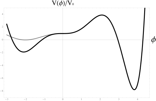
Figure 4: An example of the potential landscape consistent with the refined swampland conjecture. We show in black the example given by Eq. (34) with both minima having negative values of the cosmological constant and in gray a similar case with one of minimum located at Minkowski space. We will investigate both these scenarios later in this sections.

It is important to note that we will only be considering potentials that do not allow for inflation to be eternal around the inflection point, since the slope of the potential is not small enough. On the other hand, the critical points of our potential all satisfy the refined swampland conjecture, since the minima are located at negative (or zero) values of the cosmological constant and the maximum has a large and negative value of the slow roll parameter, $\eta=\frac{V^{\prime\prime}}{V}\approx-2$. This rules out the possibility of eternal inflation around the maximum of the potential as well.

In summary, we consider this potential to be a good representative of a swampy landscape that is in agreement with the refined swampland conjecture. In the following we will argue that a landscape like this will allow for eternal inflation, even though there is no part of the potential that permits stochastic eternal inflation. We show in Fig. 4 some potentials we will be using in the numerical examples later on in this section.

III.1 Quantum Cosmology in the Swampy Landscape

In a landscape with many dS minima and maxima, one can envision the creation of the universe from nothing as a process mediated by a dS instanton Vilenkin (1982). This instanton is the Euclideanized dS space represented by a 4-sphere of radius $1/H$. The subsequent evolution of this universe is governed by the analytically continued spacetime, which is expanding exponentially, and by possible decays of this dS state via bubble nucleation. The latter process keeps populating more states in the landscape and gives rise to a very complicated ever expanding universe with bubbles continuously being formed. In this subsection we will show that it is possible to find an instanton that describes the creation of the universe from nothing in our swampy landscape, where the potential has been severely restricted by the swampland conjectures.

Let us consider an antsatz for the Euclidean solution of the form,

$$ds^{2}=d\sigma^{2}+b^{2}(\sigma)\left(d\chi^{2}+\sin^{2}\chi d\Omega_{2}^{2}\right)~{}~{}~{};~{}~{}~{}\phi=\phi(\sigma).$$ (35)

The equations of motion for $b(\sigma)$ and $\phi(\sigma)$ are then

$$\left({{b^{\prime}}\over{b}}\right)^{2}-\left({{1}\over{b}}\right)^{2}={{1}\over{3}}\left({1\over 2}\phi^{\prime 2}-V(\phi)\right),$$ (36)

$$\phi^{\prime\prime}+{{3b^{\prime}}\over{b}}\phi^{\prime}={{dV}\over{d\phi}}.$$ (37)

We are interested in finding a compact instanton solution. In particular we can imagine that similarly to what happens in the pure dS case the metric interpolates between two points $(\sigma=0,\sigma=\sigma_{max})$, where the scale factor $b(\sigma)$ vanishes, making the instanton described by Eqs. (35) compact. This type of solution would mean that the spacetime is topologically equivalent to a deformed 4-sphere. In order to have a regular solution at those points one should impose the following conditions:

$$b^{\prime}(0)=1~{}~{}~{}~{}~{}~{}~{}~{}b^{\prime}(\sigma_{max})=-1,$$ (38)

as well as

$$\phi^{\prime}(0)=0~{}~{}~{}~{}~{}~{}~{}~{}\phi^{\prime}(\sigma_{max})=0~{}.$$ (39)

A solution with these properties can be found numerically in the potential example given above in Eq. (34). The resulting functions are shown in Figs. 5 and 6.

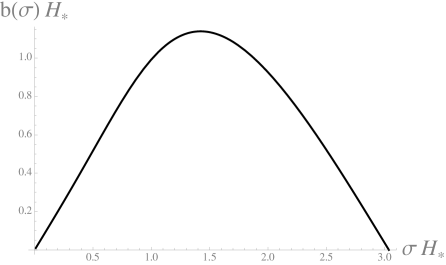
Figure 5: Solution for the scale factor for the instanton.

The solution for the scale factor is similar to the dS instanton, although it has been distorted compared to the simple dS form $b(\sigma)=H_{*}^{-1}\sin(H_{*}\sigma)$. On the other hand, the scalar field interpolates between two different points on both sides of the maximum of the potential. We note that this is possible due to the swampland conjecture that forces the scalar field curvature to be large at the top of the potential.

The evolution of the universe after its creation can be found by analytically continuing this solution to a Lorentzian signature: $\chi\rightarrow i\tau+\frac{\pi}{2}$. This substitution brings the metric to the form

$$ds^{2}=d\sigma^{2}+b^{2}(\sigma)\left(-d\tau^{2}+\cosh^{2}\tau d\Omega_{2}^{2}\right),$$ (40)

where $b(\sigma)$ and $\phi(\sigma)$ are given by the solutions obtained in the Euclidean regime. Looking at the form of this Lorentzian solution for the scalar field and the metric, one can see the similarities of this spacetime to the inflating domain wall solutions of Refs. Vilenkin (1983b); Ipser and Sikivie (1984); Widrow (1989); Basu and Vilenkin (1992). The midsection of the wall can be identified as the surface where the field crosses the maximum of the potential. This happens at a fixed value of $\sigma$, so the induced metric on that surface is that of a $(2+1)$-dimensional dS space.

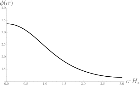
Figure 6: Scalar field solution for the instanton.

As in the domain wall spacetime, our spacetime has two horizons at $(\sigma=0,\sigma=\sigma_{max})$. The metric beyond the two horizons is that of an open FRW universe, namely

$$ds^{2}=-dt^{2}+a^{2}(t)\left(d\xi^{2}+\sinh^{2}\xi d\Omega_{2}^{2}\right),$$ (41)

where the equations of motion for $a(t)$ and $\phi(t)$ are then given by,

$$\left({{\dot{a}}\over{a}}\right)^{2}-\left({{1}\over{a}}\right)^{2}={{1}\over{3}}\left({1\over 2}{\dot{\phi}}^{2}+V(\phi)\right),$$ (42)

$${\ddot{\phi}}+{{3{\dot{a}}}\over{a}}{\dot{\phi}}=-{{dV}\over{d\phi}}.$$ (43)

The surface $t=0$ is the past light cone of the bubble wall and the initial conditions on that surface can be found by analytic continuation of the boundary conditions (38), (39): ${\dot{a}}(0)=1,~{}~{}{\dot{\phi}(0)}=0$. This implies that at small $t$ the universe is dominated by curvature, $a(t)\approx t$, while the scalar field rolls down from rest along the slopes of the potential. Focusing on the side that has the inflection point, we see that the universe will enter a quasi-deSitter stage in that region, assuming that the field is slowly rolling. One can show that the curvature dominated initial stage helps preventing a possible overshooting problem and allows the universe to enter a slow roll regime early on in the region around the inflection point Freivogel et al. (2006). This in turn means that roughly speaking the universe will expand for the maximum number of e-folds allowed for this region of the potential Blanco-Pillado et al. (2013).

The other region of spacetime, beyond the second horizon, is a bubble universe whose energy may initially be dominated by the field oscillating about the AdS minimum. The expansion will then be similar to a matter dominated universe. But eventually the negative vacuum energy takes over, the bubble universe contracts and collapses to a big crunch Abbott and Coleman (1985).

A causal diagram for the entire spacetime is shown in Fig. 7. The spacelike surface of the nucleation is denoted by $\Sigma$. The timelike thick line in the middle is the surface associated with the top of the potential. As we mentioned earlier, we can regard it as the worldsheet of an inflating domain wall. It has the geometry of a $(2+1)$-dimensional de Sitter space. The wall contracts from infinite radius, bounces and re-expands. Only the part of this diagram above the nucleation surface $\Sigma$ represents the physical spacetime. The null surfaces emanating from the endpoint of the wall worldsheet at future infinity are the bubble wall horizons. There is an FRW region on each side of the wall, and the inflating part of one of these regions is indicated by shading. Even though the wall never stops inflating, the amount of inflation is finite for comoving observers in the FRW regions and is the same for each observer (disregarding small differences due to quantum fluctuations). Slicing this spacetime with late-time Cauchy surfaces, like the surfaces represented by the horizontal dotted lines in the figure, one can see that there will always be some region of space on these slices that is inflating. Hence the creation of the universe from nothing represented by this diagram leads to eternal inflation.

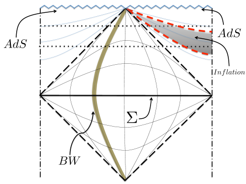
Figure 7: Causal diagram of the bubble wall universe.

In the following we will see how this picture is modified once one takes into account possible quantum fluctuations.

III.2 Bubble Wall Nucleation during Inflation

Another interpretation of the instanton (35) is that it describes a quantum decay process during inflation. In our model this would be the decay of the slow-roll inflating state by the formation of a bubble with an AdS vacuum inside. Alternatively, we can also interpret the instanton as describing quantum nucleation of a spherical domain wall during inflation Basu et al. (1991). (In our case it is actually a bubble wall.) This process can occur when $\phi$ is in the slow-roll range of the potential $V(\phi)$. The nucleation rate is

$$\lambda(\phi)\sim\exp[-I-S(\phi)],$$ (44)

where $I$ is the instanton action and $S(\phi)=3\pi/V(\phi)$ is the de Sitter entropy for the value of $\phi$ at the time of nucleation.

The instanton action in the thin wall limit (when the characteristic thickness of the wall is small compared to the horizon), $\delta\ll V_{0}^{-1/2}$, is Basu et al. (1991)

$$I_{thin}\approx 2\pi^{2}\sigma H_{\phi}^{-3}-S(\phi),$$ (45)

where $\sigma$ is the wall tension and $H_{\phi}=[V(\phi)/3]^{1/2}$. In the thick wall limit the action approaches that of the Hawking-Moss instanton Hawking and Moss (1982); Basu and Vilenkin (1992)

$$I_{thick}\approx-\pi/H_{0}^{2},$$ (46)

where $H_{0}=(V_{0}/3)^{1/2}$.

The slow roll lasts only a finite time at each comoving location, but the open universe of Eq. (40) has an infinite volume, so with a nonzero nucleation rate an infinite number of walls will be formed. Each nucleated wall will become a seed of an infinite open universe, described by the solution (40), and will also be a site of nucleation of bubble-wall universes in its slow-roll region.

III.3 Flyover wall nucleation

Inflating walls can also nucleate by the flyover mechanism. For that we need a field velocity fluctuation ${\dot{\phi}}^{2}\sim C\Delta V$ in a region of size $l\sim H^{-1}(\phi)$. Here, $\Delta V=V_{0}-V(\phi)$ is the potential difference the field needs to overcome to get to the other side of the barrier, $H(\phi)$ and $V(\phi)\sim H^{2}(\phi)$ are the expansion rate and the potential at point $\phi$ in the slow-roll region from which the nucleation occurs, and $C>1$ is a numerical factor accounting for the Hubble friction. The mass parameter in the slow-roll regime is $m\lesssim H$, so Eqs. (10) and (11) for the field velocity variance, which were derived assuming $m\gtrsim H$, do not apply here. We have estimated $\langle{\dot{\phi}}^{2}_{l}\rangle$ in this case using the method of Appendix A in Ref. Blanco-Pillado et al. (2019b), with the result

$$\langle{\dot{\phi}}^{2}\rangle\sim 10^{-2}l^{-4}\sim 10^{-2}H^{4}.$$ (47)

We thus obtain the following estimate for the flyover wall nucleation rate (assuming that $\Delta V\lesssim V_{0}$):

$$\kappa_{\rm flyover}\sim\exp\left(-10^{2}\frac{C\Delta V}{H_{0}^{4}}\right).$$ (48)

This rate can now be compared to the tunneling nucleation rate (45), (46). In the thin wall regime the wall tension can be estimated as $\sigma\sim\Delta V/m_{0}$, where $m_{0}\gtrsim H_{0}$ is the characteristic mass parameter at the top of the potential. Then the tunneling action is

$$I_{thin}+S(\phi)\sim\frac{\Delta V}{m_{0}H_{0}^{3}},$$ (49)

so the tunneling rate dominates. In the thick wall regime the tunneling action is

$$I_{thick}+S(\phi)\sim 3\pi\left(\frac{1}{V(\phi)}-\frac{1}{V_{0}}\right)\sim\frac{\pi}{3}\frac{\Delta V}{H_{0}^{4}}.$$ (50)

This has the same parametric form as (46), but the numerical coefficients suggest that tunneling is still dominant.

III.4 Spacetime structure

As we described earlier, the creation of the universe from nothing in our swampy landscape leads naturally to the formation of an inflating open patch. In the following, we will approximate this region as a flat FRW universe undergoing inflation and study the process of bubble wall nucleation within this approximation. The resulting spacetime structure is rather interesting. We will start by discussing the case where inflation ends with the scalar field settling down to a Minkowski state.

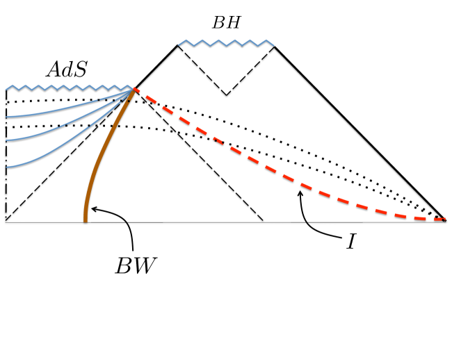
Figure 8: Causal diagram for an inflating bubble wall (BW) nucleated in an FRW inflating universe. It is assumed that inflation ends in a Minkowski vacuum. We use dashed lines for the black hole (BH) and bubble wall horizons. The thick red dashed line denoted by I, represents the spacelike surface of the end of inflation. Finally, as in the previous diagram, a couple of late time Cauchy surfaces are represented by dotted lines.

The spacetime structure in this case is illustrated in the causal diagram of Fig. 8 . Here the spacetime region in the AdS bubble interior has the same structure as in Fig. 7, and the line labeled $I$ corresponds to the end of slow roll inflation outside of the bubble. The horizontal line at the bottom is the FRW time slice of bubble nucleation. The past light cones emanating from the top of the bubble wall worldsheet represent the interior and exterior bubble wall horizons.

Notice that the dashed red line interpolates between the future infinity where the wall worldsheet ends and the spacelike infinity of the asymptotic FRW. This spacelike hypersurface has therefore a wormhole type geometry. We can see this as follows. The sphere at spacelike infinity has an infinite radius. As we go inwards along the hypersurface, the radius decreases, but then reaches a minimum and starts growing. It becomes infinite again at the top of the bubble wall worldsheet. We expect that such wormholes will later turn into black holes when their radius comes within the cosmological horizon. The inflating bubble walls will then be contained in baby universes inside of the black holes.

The necessity of black hole formation in this scenario can be understood as follows. When the wormhole is much bigger than the horizon, it evolves locally like an FRW universe. But when it comes within the horizon, it must form a singularity in about one light crossing time. Otherwise a null congruence going towards the wormhole would focus on the way in, but then defocus on the way out, which is impossible in a universe satisfying the weak energy condition ^,. The resulting spacetime is asymptotically flat, and assuming the initial wormhole is spherically symmetric, the singularity must be a black hole, by Birkhoff’s theorem. We expect the Schwarzschild radius of the black hole to be comparable to the wormhole radius at horizon crossing. Since the wall nucleation is followed by slow roll inflation, this radius is expected to be extremely large, except when the wall nucleated very close to the end of inflation. We have verified some of these expectations by performing numerical simulations described in the Appendix.

We now look at the case where the cosmological constant is negative on both sides of the wall (see Fig. 9). The main difference with the previous case is that the future evolution of the universe after inflation outside of the wall will also end up in a cosmological singularity, since the spacetime will eventually become dominated by the negative energy density of the AdS vacuum. Nonetheless, late-time Cauchy surfaces of this spacetime always include an inflating region. (A couple of such surfaces are shown by dotted lines in the figure.)

As in the previous case, the end of inflation surface in this scenario has a wormhole geometry, which may lead to the formation of a black hole. But this black hole gets eventually consumed by the big crunch singularity. This intermediate black hole is not shown in the figure.

If the landscape includes a number of domain-wall saddles with slow-roll regions, transitions between such regions would occur either by tunneling or by flyover nucleation events. As a result all habitable regions of the landscape will be populated. Depending on the shape of the potential, the flyover rate for transitions between different saddles may be higher or lower than tunneling. In some cases tunneling instantons may not exist; then flyovers provide the only transition channel.

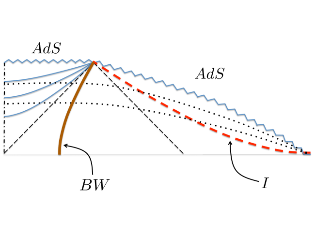
Figure 9: Same as in Fig. 8, except inflation is assumed to end in an AdS vacuum.

IV Conclusions

The swampland conjectures severely constrain the kind of low energy theories consistent with quantum gravity. These restrictions in turn have a significant impact on the possible structure of the universe at very large scales. In this paper we explored how some of these limitations can affect the presence of eternal inflation in our spacetime.

In the first part of the paper we considered the possibility of a landscape where dS states are allowed but they are greatly outnumber by AdS or Minkowski vacua. This situation seems to forbid many possible transitions between the scattered dS vacua, since there are no instanton solutions that interpolate between them. We have argued, following Ref. Brown and Dahlen (2011), that in fact there will always be transitions between the dS vacua. However, these transitions are mediated not by instantons but by quantum fluctuations of the scalar field velocity. These are the so-called flyover transitions studied recently in Ref. Blanco-Pillado et al. (2019b) (See also  Linde (1992); Ellis et al. (1990); Braden et al. (2018); Hertzberg and Yamada (2019); Huang and Ford (2019).). The fluctuations allow the field to climb over the barriers and overshoot the intervening minima, ending up in a new dS vacuum. We have studied the spacetime structure of such decays numerically and have shown that in the case of an intervening Minkowski vacuum the transition occurs by the formation of a baby universe connected to the parent FRW spacetime by a wormhole. The wormhole eventually collapses, leaving behind a black hole. For an intervening AdS vacuum, an expanding shell-like region surrounding the new baby universe collapses to a big crunch. From the exterior parent vacuum this region is seen as an expanding AdS bubble. Our conclusion is that a landscape with overwhelming majority of AdS or Minkowski vacua still leads to an eternally inflating multiverse, with inflating pocket universes hidden behind black hole horizons or in AdS bubbles.

We have also studied the impact that this type of landscape architecture would have on the predictions for the value of the cosmological constant. We find that the requirements for a successful prediction can be easily accommodated in a landscape with a very small fraction of dS vacua.

In the second part of the paper we investigated a more restrictive type of landscape, suggested by the so-called refined swampland conjecture. This conjecture does not allow dS maxima or saddle points that are flat enough for hilltop inflation. In order to accommodate inflation in this landscape, we assume that slow roll regions can be found around inflection points on the slopes of the potential, while all minima are either AdS or Minkowski. All these restrictions make the usual stochastic eternal inflation nearly impossible, except perhaps in marginal cases Matsui and Takahashi (2019); Dimopoulos (2018); Kinney (2019); Brahma and Shandera (2019); Wang et al. (2019).

We studied quantum creation of the universe from nothing in a restricted landscape of this kind and identified the instanton configuration corresponding to this process. The Lorentzian continuation of this instanton describes an AdS or Minkowski bubble bounded by an inflating bubble wall, where the wall inflation continues all the way to future infinity.

The same instanton describes the process of quantum bubble wall nucleation during inflation. These walls are associated with the high curvature saddle points of the potential which are allowed by the refined conjecture. Once formed the walls will inflate forever, spawning new inflationary regions as the field rolls down the slope of the potential. Wall nucleation can also occur by non-instanton flyover transitions. We studied in detail the resulting spacetime structure with the help of some numerical simulations. Similarly to what happens in related models like Garriga et al. (2016); Deng and Vilenkin (2017), the expansion of the walls in this background leads to a wormhole geometry. If after inflation the field rolls into a Minkowski vacuum, the wormhole eventually collapses to a black hole, and the inflating wall ends up in a baby universe hidden behind the black hole horizon. Alternatively, if the field rolls into an AdS minimum, the region outside of the wall eventually collapses to a big crunch. In either case the wall inflation continues forever and an unlimited number of inflating walls is ultimately formed. These processes lead to a complicated global structure of an eternally inflating multiverse.

In conclusion, we have explored the implications of different landscapes suggested by the swampland conjectures and showed how they always lead to the formation of new inflating regions, sometimes hidden behind black hole horizons or inside of AdS bubbles. This suggests that eternal inflation is a robust conclusion even for swampy landscapes, although the specific structure of spacetime for each landscape architecture could be quite different.

V Acknowledgements

We are grateful to Ken Olum for useful discussions. J. J. B.-P. is supported in part by the Spanish Ministry MINECO grant (FPA2015-64041-C2-1P), the MCIU/AEI/FEDER grant (PGC2018-094626-B-C21), the Basque Government grant (IT-979-16) and the Basque Foundation for Science (IKERBASQUE). H. D. and A. V. are supported in part by the National Science Foundation under grant PHY-1820872.

Appendix A Wormhole evolution

As discussed in Subsec. III D, after the AdS bubble is formed, the bubble wall grows into a region connected to the exterior FRW universe through a wormhole geometry. The wormhole radius is initially super-horizon, but it eventually comes within the horizon, and we expect that the wormhole turns into a black hole soon thereafter. The Schwarzschild radius of the black hole is expected to be comparable to the wormhole radius at horizon crossing. In this Appendix we verify these expectations by numerical simulations in a simplified setting of a radiation dominated universe with a wormhole geometry.

Consider a general, spherically symmetric metric

$$ds^{2}=-dt^{2}+B^{2}dr^{2}+R^{2}d\Omega^{2},$$ (51)

where $d\Omega^{2}$ is the line element on a unit sphere and $B$ and $R$ (which is called the area radius) are functions of the coordinates $t$ and $r$.

The matter content in a radiation-dominated universe can be described by a perfect fluid with energy-momentum tensor $T_{\mu\nu}=\rho\left(4u_{\mu}u_{\nu}+g_{\mu\nu}\right)/3$, where $\rho(r,t)$ is the energy density measured in the fluid frame. The fluid’s 4-velocity $u^{\mu}(r,t)$ can be written in the form

$$u^{\mu}=\left(\frac{1}{\sqrt{1-v^{2}}},\frac{v}{B\sqrt{1-v^{2}}},0,0\right)$$ (52)

where $v(r,t)$ is the fluid’s 3-velocity relative to the comoving coordinate $r$.

Let $H_{i}$ be the cosmological expansion rate far from the wormhole, where the metric is close to FRW, at the initial time of the simulation. By the following replacements,

$$t\to H_{i}^{-1}t,\ B\to H_{i}^{-1}B,\ R\to H_{i}^{-1}R,\ \rho\to H_{i}^{2}\rho/G,$$ (53)

all variables become dimensionless.

Our goal is to solve the Einstein equations in order to find out the evolution of the metric functions and the fluid.

For later convenience, we define

$$U=\dot{R},\ \ \ \ \Gamma=\frac{R^{\prime}}{B},\ \ \ \ K=\frac{\dot{B}}{B}+\frac{2\dot{R}}{R},$$ (54)

where $\dot{}\equiv{\partial}/{\partial t}$ and ${}^{\prime}\equiv{\partial}/{\partial r}$.

The Einstein equations then take the form

$$\dot{K}=-\left(K-\frac{2U}{R}\right)^{2}-2\left(\frac{U}{R}\right)^{2}-4\pi(T_{00}+T_{\ 1}^{1}+2T_{\ 2}^{2})$$ (55)

$$\dot{U}=-\frac{1-\Gamma^{2}+U^{2}}{2R}-4\pi RT_{\ 1}^{1}$$ (56)

$$\dot{\Gamma}=-\frac{4\pi RT_{\ 1}^{0}}{B}$$ (57)

$$\dot{\rho}=-\frac{4\rho}{3-v^{2}}\left[\left(1-v^{2}\right)K+2v^{2}\frac{U}{R}+2v\frac{\Gamma}{R}+\frac{v^{\prime}}{B}\right]-\frac{2}{3-v^{2}}\frac{\rho^{\prime}v}{B},$$ (58)

$$\dot{v}=-\frac{(1-v^{2})}{3-v^{2}}\left[2v\left(K-\frac{3U}{R}\right)-2v^{2}\frac{\Gamma}{R}+\frac{3(1-v^{2})\rho^{\prime}}{4\rho B}\right]-\frac{2}{3-v^{2}}\frac{v^{\prime}v}{B},$$ (59)

$$\dot{B}=B\left(K-\frac{2U}{R}\right),$$ (60)

$$\dot{R}=U,$$ (61)

where

$$T_{00}=\frac{3+v^{2}}{3-3v^{2}}\rho,$$ (62)

$$T_{\ 1}^{1}=\frac{1+3v^{2}}{3-3v^{2}}\rho,$$ (63)

$$T_{\ 2}^{2}=\frac{1}{3}\rho,$$ (64)

$$T_{\ 1}^{0}=-\frac{4\rho vB}{3-3v^{2}}.$$ (65)

To evolve this system, we need initial and boundary conditions. Without loss of generality, let $t_{i}=1/2$ be the initial time of the simulation, so the initial Hubble radius is $1/H_{i}=1$. We then set $B=1$, $\rho=3/32\pi t_{i}^{2}=3/8\pi$ and $v=0$ at $t_{i}$. To enforce a wormhole configuration at $t_{i}$, we require a wormhole throat at $r=0$, i.e., $R^{\prime}=0$. On the other hand, we need a flat FRW universe far from the wormhole, i.e., $R=ar$, where $a=\left(t/t_{i}\right)^{1/2}$ is the FRW scale factor. The initial profile of $R$ is thus chosen to be

$$R(r)=\left(r^{b}+r_{0}^{b}\right)^{1/b},$$ (66)

where $b\geq 2$. This function satisfies $R^{\prime}=0$ at $r=0$, and $R\approx r$ at $r\gg r_{0}$. In simulations we set $b\gg 1$ (e.g., $b=10$) such that $R\approx r$ at $r>r_{0}$, which means the FRW universe is immediately realized outside of $r=r_{0}$. We are interested in superhorizonal wormholes at $t_{i}$, so $r_{0}>1$.

By definition, the initial profile of $\Gamma$ is

$$\Gamma(r)=\frac{r^{b-1}}{r^{b}+r_{0}^{b}}R.$$ (67)

The mass of the central object can be characterized by the quasi-local Misner-Sharp mass, which in our coordinates is

$$M=\frac{R}{2}\left(1-\Gamma^{2}+U^{2}\right).$$ (68)

From $G_{00}=8\pi T_{00}$, we have $M^{\prime}(r)=4\pi\rho R^{2}R^{\prime}$, which gives $M(r)=R^{3}/2$ at $t_{i}$. By the definition of $M$, we can also find the initial profile of $U$,

$$U(r)=\sqrt{\Gamma^{2}+R^{2}-1}.$$ (69)

From $G_{01}=8\pi T_{01}$, it can be shown that

$$\frac{\dot{B}}{B}=\frac{U^{\prime}}{R^{\prime}}=\frac{dU}{dR}=\frac{(b-1)\left(r_{0}/R^{2}\right)^{b}r^{b-2}+1}{U/R}.$$ (70)

Therefore, by definition, the initial profile of $K$ is

$$K(r)=\frac{(b-1)\left(r_{0}/R^{2}\right)^{b}r^{b-2}+1}{U/R}+\frac{2U}{R}.$$ (71)

Following this procedure we obtain all the initial conditions needed for our system of equations. The boundary conditions are simply $\rho^{\prime}(r=0,t)=v^{\prime}(r=0,t)=0.$

The formation of a black hole can be indicated by the appearance of a black hole apparent horizon, where we have

$$U+\Gamma=0,\ \ \ \ U-\Gamma<0$$ (72)

in our coordinates. Then the black hole mass can be read as the Misner-Sharp mass on the horizon, $M=R/2$. More details can be found in Ref. Deng and Vilenkin (2017) and references therein.

In all our simulations with different values of $r_{0}$, the wormholes eventually turn into black holes. As explained in Subsec. III D, we expect that this happens soon after the wormhole comes within the cosmological horzion. In our units the horizon crossing time is found to be $t_{H}=r_{0}^{2}/4t_{i}=r_{0}^{2}/2$. Furthermore, it is expected that the Schwarzschild radius of the black hole is comparable to the wormhole radius at horizon crossing. Fig. 10 shows the black hole formation times $t_{BH}$ for several cases with different values of $r_{0}$. It is found that $t_{BH}\approx 2.8t_{H}.$ Fig. 11 shows the relation between the Schwarzschild radius of the black hole $R_{BH}$ and the horizon crossing radius of the wormhole, $R_{H}=2t_{H}=r_{0}^{2}$. It is found that $R_{BH}\approx 1.2R_{H}.$

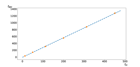
Figure 10: Relation between the horizon crossing time $t_{H}$ and the black hole formation time $t_{BH}$. The dots are from simulations with $r_{0}=5,10,15,20,25,30$. The dashed line is the best fit of the data. The slope is approximately 2.8.

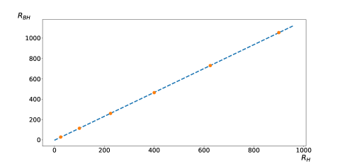
Figure 11: Relation between the wormhole radius at horizon crossing $R_{H}$ and the black hole radius $R_{BH}$. The dots are from simulations with $r_{0}=5,10,15,20,25,30$. The dashed line is the best fit of the data. The slope is approximately 1.2.

References

- Bousso and Polchinski (2000) R. Bousso and J. Polchinski, JHEP 06, 006 (2000), eprint hep-th/0004134.
- Susskind (2003) L. Susskind, pp. 247–266 (2003), eprint hep-th/0302219.
- Douglas (2003) M. R. Douglas, JHEP 05, 046 (2003), eprint hep-th/0303194.
- Kachru et al. (2003) S. Kachru, R. Kallosh, A. D. Linde, and S. P. Trivedi, Phys. Rev. D68, 046005 (2003), eprint hep-th/0301240.
- Denef and Douglas (2004) F. Denef and M. R. Douglas, JHEP 05, 072 (2004), eprint hep-th/0404116.
- Douglas and Kachru (2007) M. R. Douglas and S. Kachru, Rev. Mod. Phys. 79, 733 (2007), eprint hep-th/0610102.
- Vilenkin (1983a) A. Vilenkin, Phys. Rev. D27, 2848 (1983a).
- Starobinsky (1986) A. A. Starobinsky, Lect. Notes Phys. 246, 107 (1986).
- Linde (1992) A. D. Linde, Nucl. Phys. B372, 421 (1992), eprint hep-th/9110037.
- Obied et al. (2018) G. Obied, H. Ooguri, L. Spodyneiko, and C. Vafa (2018), eprint 1806.08362.
- Agrawal et al. (2018) P. Agrawal, G. Obied, P. J. Steinhardt, and C. Vafa, Phys. Lett. B784, 271 (2018), eprint 1806.09718.
- Achucarro and Palma (2019) A. Achucarro and G. A. Palma, JCAP 1902, 041 (2019), eprint 1807.04390.
- Kehagias and Riotto (2018) A. Kehagias and A. Riotto, Fortsch. Phys. 66, 1800052 (2018), eprint 1807.05445.
- Kinney et al. (2019) W. H. Kinney, S. Vagnozzi, and L. Visinelli, Class. Quant. Grav. 36, 117001 (2019), eprint 1808.06424.
- Garg and Krishnan (2018) S. K. Garg and C. Krishnan (2018), eprint 1807.05193.
- Dias et al. (2019) M. Dias, J. Frazer, A. Retolaza, and A. Westphal, Fortsch. Phys. 67, 2 (2019), eprint 1807.06579.
- Das (2019) S. Das, Phys. Rev. D99, 083510 (2019), eprint 1809.03962.
- Denef et al. (2018) F. Denef, A. Hebecker, and T. Wrase, Phys. Rev. D98, 086004 (2018), eprint 1807.06581.
- Choi et al. (2018) K. Choi, D. Chway, and C. S. Shin, JHEP 11, 142 (2018), eprint 1809.01475.
- Murayama et al. (2018) H. Murayama, M. Yamazaki, and T. T. Yanagida, JHEP 12, 032 (2018), eprint 1809.00478.
- Conlon (2018) J. P. Conlon, Int. J. Mod. Phys. A33, 1850178 (2018), eprint 1808.05040.
- Blanco-Pillado et al. (2019a) J. J. Blanco-Pillado, M. A. Urkiola, and J. M. Wachter, JHEP 01, 187 (2019a), eprint 1811.05463.
- Olguin-Trejo et al. (2019) Y. Olguin-Trejo, S. L. Parameswaran, G. Tasinato, and I. Zavala, JCAP 1901, 031 (2019), eprint 1810.08634.
- Ooguri et al. (2019) H. Ooguri, E. Palti, G. Shiu, and C. Vafa, Phys. Lett. B788, 180 (2019), eprint 1810.05506.
- Garg et al. (2019) S. K. Garg, C. Krishnan, and M. Zaid Zaz, JHEP 03, 029 (2019), eprint 1810.09406.
- Andriot (2018) D. Andriot, Phys. Lett. B785, 570 (2018), eprint 1806.10999.
- Motaharfar et al. (2019) M. Motaharfar, V. Kamali, and R. O. Ramos, Phys. Rev. D99, 063513 (2019), eprint 1810.02816.
- Ashoorioon (2019) A. Ashoorioon, Phys. Lett. B790, 568 (2019), eprint 1810.04001.
- Heckman et al. (2019) J. J. Heckman, C. Lawrie, L. Lin, J. Sakstein, and G. Zoccarato (2019), eprint 1901.10489.
- Matsui and Takahashi (2019) H. Matsui and F. Takahashi, Phys. Rev. D99, 023533 (2019), eprint 1807.11938.
- Dimopoulos (2018) K. Dimopoulos, Phys. Rev. D98, 123516 (2018), eprint 1810.03438.
- Kinney (2019) W. H. Kinney, Phys. Rev. Lett. 122, 081302 (2019), eprint 1811.11698.
- Brahma and Shandera (2019) S. Brahma and S. Shandera (2019), eprint 1904.10979.
- Wang et al. (2019) Z. Wang, R. Brandenberger, and L. Heisenberg (2019), eprint 1907.08943.
- Dvali and Gomez (2019) G. Dvali and C. Gomez, Fortsch. Phys. 67, 1800092 (2019), eprint 1806.10877.
- Dvali et al. (2019) G. Dvali, C. Gomez, and S. Zell, Fortsch. Phys. 67, 1800094 (2019), eprint 1810.11002.
- Rudelius (2020) T. Rudelius, JCAP 2019, 009 (2020), eprint 1905.05198.
- Kallosh et al. (2019) R. Kallosh, A. Linde, E. McDonough, and M. Scalisi, JHEP 03, 134 (2019), eprint 1901.02022.
- Akrami et al. (2019) Y. Akrami, R. Kallosh, A. Linde, and V. Vardanyan, Fortsch. Phys. 67, 1800075 (2019), eprint 1808.09440.
- Dine and Paban (2015) M. Dine and S. Paban, JHEP 10, 088 (2015), eprint 1506.06428.
- Yamada and Vilenkin (2018) M. Yamada and A. Vilenkin, JHEP 03, 029 (2018), eprint 1712.01282.
- Brown and Dahlen (2010) A. R. Brown and A. Dahlen, Phys. Rev. D82, 083519 (2010), eprint 1004.3994.
- Clifton et al. (2007) T. Clifton, A. D. Linde, and N. Sivanandam, JHEP 02, 024 (2007), eprint hep-th/0701083.
- Johnson and Yang (2010) M. C. Johnson and I.-S. Yang, Phys. Rev. D82, 065023 (2010), eprint 1005.3506.
- Brown and Dahlen (2011) A. R. Brown and A. Dahlen, Phys. Rev. Lett. 107, 171301 (2011), eprint 1108.0119.
- Blanco-Pillado et al. (2019b) J. J. Blanco-Pillado, H. Deng, and A. Vilenkin (2019b), eprint 1906.09657.
- Ellis et al. (1990) J. R. Ellis, A. D. Linde, and M. Sher, Phys. Lett. B252, 203 (1990).
- Braden et al. (2018) J. Braden, M. C. Johnson, H. V. Peiris, A. Pontzen, and S. Weinfurtner (2018), eprint 1806.06069.
- Hertzberg and Yamada (2019) M. P. Hertzberg and M. Yamada (2019), eprint 1904.08565.
- Huang and Ford (2019) H. Huang and L. Ford (2019), work in progress. Seminar given by H. Huang at Tufts University, April 2018.
- Deng et al. (2017) H. Deng, J. Garriga, and A. Vilenkin, JCAP 1704, 050 (2017), eprint 1612.03753.
- Deng and Vilenkin (2017) H. Deng and A. Vilenkin, JCAP 1712, 044 (2017), eprint 1710.02865.
- Freivogel (2011) B. Freivogel, Class. Quant. Grav. 28, 204007 (2011), eprint 1105.0244.
- Linde and Mezhlumian (1993) A. D. Linde and A. Mezhlumian, Phys. Lett. B307, 25 (1993), eprint gr-qc/9304015.
- Linde et al. (1994) A. D. Linde, D. A. Linde, and A. Mezhlumian, Phys. Rev. D49, 1783 (1994), eprint gr-qc/9306035.
- De Simone et al. (2008) A. De Simone, A. H. Guth, M. P. Salem, and A. Vilenkin, Phys. Rev. D78, 063520 (2008), eprint 0805.2173.
- Bousso et al. (2009) R. Bousso, B. Freivogel, and I.-S. Yang, Phys. Rev. D79, 063513 (2009), eprint 0808.3770.
- Schwartz-Perlov and Vilenkin (2006) D. Schwartz-Perlov and A. Vilenkin, JCAP 0606, 010 (2006), eprint hep-th/0601162.
- Garriga et al. (2006) J. Garriga, D. Schwartz-Perlov, A. Vilenkin, and S. Winitzki, JCAP 0601, 017 (2006), eprint hep-th/0509184.
- Schwartz-Perlov and Vilenkin (2010) D. Schwartz-Perlov and A. Vilenkin, JCAP 1006, 024 (2010), eprint 1004.4567.
- Dvali and Vilenkin (2004) G. Dvali and A. Vilenkin, Phys. Rev. D70, 063501 (2004), eprint hep-th/0304043.
- Dvali (2006) G. Dvali, Phys. Rev. D74, 025018 (2006), eprint hep-th/0410286.
- Basu and Vilenkin (1992) R. Basu and A. Vilenkin, Phys. Rev. D46, 2345 (1992).
- Basu and Vilenkin (1994) R. Basu and A. Vilenkin, Phys. Rev. D50, 7150 (1994), eprint gr-qc/9402040.
- Vilenkin (1994) A. Vilenkin, Phys. Rev. Lett. 72, 3137 (1994), eprint hep-th/9402085.
- Linde (1994) A. D. Linde, Phys. Lett. B327, 208 (1994), eprint astro-ph/9402031.
- Vilenkin (1982) A. Vilenkin, Phys. Lett. 117B, 25 (1982).
- Garriga and Sasaki (2000) J. Garriga and M. Sasaki, Phys. Rev. D62, 043523 (2000), eprint hep-th/9912118.
- Vilenkin (1983b) A. Vilenkin, Phys. Lett. 133B, 177 (1983b).
- Ipser and Sikivie (1984) J. Ipser and P. Sikivie, Phys. Rev. D30, 712 (1984).
- Widrow (1989) L. M. Widrow, Phys. Rev. D39, 3571 (1989).
- Freivogel et al. (2006) B. Freivogel, M. Kleban, M. Rodriguez Martinez, and L. Susskind, JHEP 03, 039 (2006), eprint hep-th/0505232.
- Blanco-Pillado et al. (2013) J. J. Blanco-Pillado, M. Gomez-Reino, and K. Metallinos, JCAP 1302, 034 (2013), eprint 1209.0796.
- Abbott and Coleman (1985) L. F. Abbott and S. R. Coleman, Nucl. Phys. B259, 170 (1985).
- Basu et al. (1991) R. Basu, A. H. Guth, and A. Vilenkin, Phys. Rev. D44, 340 (1991).
- Hawking and Moss (1982) S. W. Hawking and I. G. Moss, Phys. Lett. 110B, 35 (1982), [Adv. Ser. Astrophys. Cosmol.3,154(1987)].
- Coleman and De Luccia (1980) S. R. Coleman and F. De Luccia, Phys. Rev. D21, 3305 (1980).
- Hawking and Ellis (2011) S. W. Hawking and G. F. R. Ellis, The Large Scale Structure of Space-Time, Cambridge Monographs on Mathematical Physics (Cambridge University Press, 2011), ISBN 9780521200165, 9780521099066, 9780511826306, 9780521099066.
- Geroch (1967) R. P. Geroch, J. Math. Phys. 8, 782 (1967).
- Garriga et al. (2016) J. Garriga, A. Vilenkin, and J. Zhang, JCAP 1602, 064 (2016), eprint 1512.01819.