Note on the Power-2 Limb Darkening Law

1

Limb darkening laws are simple formulae that approximate the stellar intensity $I_{\lambda}$ as function of the foreshortening angle $\mu$ measured from the center of the stellar disk (i.e. $\mu\equiv\cos{\theta}$ where $\theta$ is the angle between the line of sight and the surface normal). Recently there has been a renewed interest in the power-2 law for modeling exoplanet transits (e.g. Maxted (2018), Maxted & Gill (2019)) because it provides a better match to the stellar intensities generated by spherical stellar atmosphere models than other 2-parameter laws (Morello et al., 2017). Accuracy in modeling the limb darkening is particularly important when attempting to measure unbiased exoplanetary radii (e.g. Espinoza & Jordán (2015), Neilson et al. (2017)) and higher-order effects such as tidal deformation (Akinsanmi et al., 2019). We agree with the above cited works and so to help facilitate wider use of the power-2 law, we correct a minor error and expand on the work of Maxted (2018).

In the power-2 law (see Hestroffer (1997)) the specific intensity, $I$, is defined as

$$\begin{aligned} I(\mu)=1-c\big{(}1-\mu^{\alpha}\big{)}~{}~{}~{}~{}~{}~{}~{}~{}\alpha>0,~{}~{}~{}0\leq\mu\leq 1.\end{aligned}$$ (1)

Maxted (2018) found that $c$ and $\alpha$ are highly correlated when modeling transit light curves, so to enable more efficient sampling he introduced the parameters $h_{1}\equiv I$($\mu$=0.5) and $h_{2}\equiv h_{1}-I$($\mu$=0) in place of $c$ and $\alpha$. These are related to $c$ and $\alpha$ by

$$\begin{aligned} &h_{1}=1-c\big{(}1-2^{-\alpha}\big{)}\\ &h_{2}=c2^{-\alpha}\end{aligned}$$ (2)

and the inverse

$$\begin{aligned} &c=1-h_{1}+h_{2}\\ &\alpha=\log_{2}\bigg{(}\frac{c}{h_{2}}\bigg{)}.\end{aligned}$$ (3)

Maxted (2018) further stated that “These definitions impose the constraints $h_{1}<1$ and $\bf{h_{1}+h_{2}\leq 1}$ that are required so that the flux is positive at all points on the stellar disc.” Unfortunately, the inequality highlighted in bold does not, in fact, satisfy that condition. For example, if we choose $h_{1}=0.25$ and $h_{2}=0.50$ this gives $I(0)=-0.25$, an unphysical negative intensity at the center of the stellar disk. Below we provide a derivation of the actual realizable region in the $(h_{1},h_{2})$ plane – a triangular area obeying the inequalities $h_{1}<1$ and $0<h_{2}\leq h_{1}$. Knowing the allowed region of the power-2 limb darkening parameter space is important for Bayesian parameter estimation techniques, such as the various flavors of MCMC, since these methods require proper sampling of the priors.

Following Kipping (2013), the necessary physical constraints on $I$ are

$$\begin{aligned} &{\rm Condition\ A:}\ I(\mu)\geq 0\\ &{\rm Condition\ B:}\ I(\mu)\text{ is a strictly increasing function (from limb to center)}\end{aligned}$$ (4)

Note that conditions A and B imply that the $h_{1}$ and $h_{2}$ parameters are positive. The function $\mu^{\alpha}$ is a root for $0<\alpha<1$ and a power for $\alpha\geq 1$. In both cases, $\mu^{\alpha}$ is an increasing function, and the $min_{\mu}~{}\mu^{\alpha}=0$. If $c>0$ then $c\mu^{\alpha}$ is strictly increasing; otherwise, if $c<0$ then $c\mu^{\alpha}$ is decreasing. Condition B thus implies that $c>0$. Condition A implies

$$\begin{aligned} I(\mu)\geq min_{\mu}I(\mu)=1-c+min_{\mu}(c\mu^{\alpha})=1-c\geq 0~{}~{}~{}\Rightarrow c\leq 1\end{aligned}$$ (5)

The region in the $(c,\alpha)$ plane is thus the semi-infinite strip given by $0<c\leq 1$ and $\alpha>0$. The region boundaries in the $(c,\alpha)$ plane then imply a restriction in the $(h_{1},h_{2})$ plane:

$$1\geq c~{}~{}\Rightarrow~{}~{}1\geq 1-h_{1}+h_{2}~{}~{}~{}\Rightarrow~{}~{}h_{1}\geq h_{2}$$ (6)

$$\alpha>0~{}~{}\Rightarrow~{}~{}\log_{2}{\bigg{(}\frac{c}{h_{2}}\bigg{)}}>0~{}~{}\Rightarrow\frac{c}{h_{2}}>1~{}~{}~{}\Rightarrow~{}~{}c>h_{2}$$ (7)

$$c>h_{2}~{}~{}\Rightarrow~{}~{}(1-h_{1}+h_{2})>h_{2}~{}~{}~{}\Rightarrow~{}~{}1>h_{1}$$ (8)

Thus, the region in the $(h_{1},h_{2})$ plane is triangular and given by the inequalities

$$h_{1}>0,~{}~{}h_{2}>0,~{}~{}h_{2}\leq h_{1},~{}~{}\text{and}~{}h_{1}<1.$$ (9)

For MCMC methods, efficient sampling of the prior can be extremely important. A new set of parameters can be defined which transforms the ($h_{1}$, $h_{2}$) triangular region into the unit square, preserving the uniform sampling property. Such a transformation can be obtained by following the prescription given by Kipping (2013):

$$\begin{aligned} &q_{1}=(1-h_{2})^{2}\\ &q_{2}=(h_{1}-h_{2})/(1-h_{2})\\ &{\rm for}~{}~{}0<q_{1}<1,~{}~{}~{}0\leq q_{2}<1\end{aligned}$$ (10)

with the inverse transformation given by:

$$\begin{aligned} &h_{1}=1-\sqrt{q_{1}}+q_{2}\sqrt{q_{1}}\\ &h_{2}=1-\sqrt{q_{1}}.\end{aligned}$$ (11)

Finally, the parameters $c$ and $\alpha$ can then be written in terms of $q_{1}$ and $q_{2}$:

$$\begin{aligned} &c=1-q_{2}\sqrt{q_{1}}\\ &\alpha=\log_{2}\bigg{(}\frac{1-q_{2}\sqrt{q_{1}}}{1-\sqrt{q_{1}}}\bigg{)}=3.3219\log{\bigg{(}\frac{1-q_{2}\sqrt{q_{1}}}{1-\sqrt{q_{1}}}\bigg{)}.}\end{aligned}$$ (12)

Figure 1 shows the allowable regions for the power-2 law coefficients in the Kipping, Maxted, and original Hestroffer formulations. Note that while the triangular region defined by $h_{1}$ and $h_{2}$ is permitted by the power-2 law parameterization and conditions on $I$, not all allowed locations in the region are a priori equally likely. Some areas correspond to intensity distributions that may not be realized in actual stellar atmospheres. For example, using the 3D stagger-grid (Magic et al., 2015) of stellar atmosphere models for cool stars, Maxted (2018) finds no cases outside the ranges $0.37<h_{1}<0.87$ or $0.25<h_{2}<0.78$ for unspotted stars. This corresponds to a significantly smaller region than the unit square in the ($q_{1}$, $q_{2}$) plane, and a greatly reduced area in the ($c$, $\alpha$) plane. Such limits can be imposed by placing appropriate constraints on the priors.

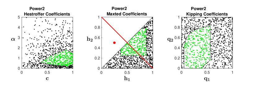
Figure 1: The figure shows the limb darkening coefficients for the power-2 law. The left panel shows a small region of the semi-infinite strip corresponding to the Hestroffer $c$ and $\alpha$ coefficients. The middle panel shows the triangular region using the Maxted $h_{1}$ and $h_{2}$ coefficients. Note that the red line is an incorrect bounding line segment and the red point at ($h_{1}$=0.25, $h_{2}$=0.5) resides outside the physically allowed region. The right panel shows the ($q_{1}$, $q_{2}$) unit square in the Kipping parameterization. The dots show 1000 uniform samples randomly chosen from the ($q_{1}$, $q_{2}$) unit square, and then cast into the Maxted and Hestroffer regions. The green colored dots correspond to the more likely pairs of coefficients, based on stellar atmosphere models as found in Maxted (2018).