Shearing in the space of adelic lattices

Abstract.

In this notes we show how a problem regarding continued fractions of rational numbers, lead to several phenomena in number theory and dynamics, and eventually to the problem of shearing of divergent diagonal orbits in the space of adelic lattices. Finding these ideas quite interesting, the first half of these notes is about explaining theses ideas, the intuition and motivation behind them, and the second contains the details and proofs.

1. Introduction

1.1. The main results

The connection between number theory and homogeneous dynamics is well established - many problems in number theory have found elegant formulations and solutions in the language of homogeneous dynamics, and in particular the dynamics of the space of unimodular Euclidean lattices $\mathrm{SL}_{n}\left(\mathbb{Z}\right)\backslash\mathrm{SL}_{n}\left(\mathbb{R}\right)$. One of the main examples, which led eventually to this paper, is the problem of finding good Diophantine approximations.

It is well known that these rational approximations can be read as the prefixes of the continued fraction expansion of any given number

$$x=\left[a_{0};a_{1},a_{2},...\right]=a_{0}+\frac{1}{a_{1}+\frac{1}{a_{2}+\ddots}}.$$

This continued fraction presentation comes with the natural Gauss map, which is simply the shift left map $T\left(\left[0;a_{1},a_{2},a_{3},...\right]\right):=\left[0;a_{2},a_{3},...\right]$ (or equivalently $T\left(x\right):=\frac{1}{x}-\left\lfloor\frac{1}{x}\right\rfloor$), and many problems in Diophantine approximation are studied via this map. In particular, one of the mail tools in this area is the ergodicity of this map with respect to the Gauss measure $\nu_{\mathrm{Gauss}}=\frac{1}{\ln\left(2\right)}\cdot\frac{1}{1+t}\cdot\mathrm{dt}$. This allows us to use the Pointwise Ergodic Theorem, which states that almost every $x\in\left[0,1\right]$ is generic, namely for every continuous function $f:\left[0,1\right]\to\mathbb{R}$ we have that

$$\frac{1}{N}\sum_{0}^{N-1}f\left(T^{i}\left(x\right)\right)\to\nu_{\mathrm{Gauss}}\left(f\right)=\frac{1}{\ln\left(2\right)}\int_{0}^{1}f\left(t\right)\frac{1}{1+t}\mathrm{dt}.$$

In this case we say that the $T$-orbit of $x$ equidistributes. However, this is not true in general, and in particular this fails for rational $x$ which has a finite continued fraction expansion. In this case (and in others as well), instead of studying an orbit of a single point $x$, we usually study the “finite” orbits of certain naturally defined finite families $\mathcal{F}_{i}$ of points (and in this paper the families of rationals $\left\{\frac{p}{q}\;\mid\;1\leq p\leq q,\;\left(p,q\right)=1\right\}$ for $q\in\mathbb{N}$). Then, our question is if taking the orbits of each family together, do they equidistribute as $i\to\infty$.

It is well known that any $T$-orbit has a continuous analogue as an orbit of the diagonal subgroup $A\leq\mathrm{SL}_{2}\left(\mathbb{R}\right)$ in $\mathrm{SL}_{2}\left(\mathbb{Z}\right)\backslash\mathrm{SL}_{2}\left(\mathbb{R}\right)$. We can reformulate the problem above in this new continuous language, where the “finite” orbits become divergent $A$-orbits. This already give us more tools to work with, and in particular we can use unipotent flows which are much more understood than $A$-flows.

As it turns out, an even more natural point of view for this kind of questions is actually over the Adeles, where these finite families of $A$-orbits are combined together to a translation of a single orbit of the diagonal matrices over the adeles $\mathbb{A}$, which is known in the literature as the shearing process.

In this notes we show that these translations of a single orbit over the adeles through the origin always equidistribute, as long as there are no trivial reasons for them not to, or formally we have the following.

Theorem 1.

Let $X_{\mathbb{A}}=\Gamma_{\mathbb{A}}\backslash G_{\mathbb{A}}$ where $\Gamma_{\mathbb{A}}=\mathrm{GL}_{2}\left(\mathbb{Q}\right)$ and

$$G_{\mathbb{A}} =\left\{\left(g^{\left(\infty\right)},g^{\left(2\right)},g^{\left(3\right)},...\right)\in\mathrm{GL}_{2}\left(\mathbb{A}\right)\;\mid\;\prod_{\nu}\left|\det\left(g^{\left(\nu\right)}\right)\right|_{\nu}=1\right\}.$$

Denote by $A_{\mathbb{A}}\leq G_{\mathbb{A}}$ the diagonal subgroup and let $\delta_{\Gamma_{\mathbb{A}}A_{\mathbb{A}}}$ be the $A_{\mathbb{A}}$-invariant orbit measure on $\Gamma_{\mathbb{A}}A_{\mathbb{A}}$. Then for any sequence $g_{i}\in G_{\mathbb{A}}$ such that $g_{i}/A_{\mathbb{A}}$ diverges in $\nicefrac{{G_{\mathbb{A}}}}{{A_{\mathbb{A}}}}$, the sequence $g_{i}\left(\delta_{\Gamma_{\mathbb{A}}A_{\mathbb{A}}}\right)$ equidistributes, i.e. for any $f_{1},f_{2}\in C_{c}\left(X_{\mathbb{A}}\right)$ with $\mu_{Haar,\mathbb{A}}\left(f_{2}\right)\neq 0$ we have that

$$\frac{\left(g_{i}\delta_{\Gamma_{\mathbb{A}}A_{\mathbb{A}}}\right)\left(f_{1}\right)}{\left(g_{i}\delta_{\Gamma_{\mathbb{A}}A_{\mathbb{A}}}\right)\left(f_{2}\right)}\to\frac{\mu_{Haar,\mathbb{A}}\left(f_{1}\right)}{\mu_{Haar,\mathbb{A}}\left(f_{2}\right)}.$$

Once the theorem above is proved over the adeles, we automatically obtain similar results for spaces which are defined naturally as projections of $X_{\mathbb{A}}$ (see 8.1 for the definition). One of the main examples is the space of unimodular lattices $X_{\mathbb{R}}=\mathrm{SL}_{2}\left(\mathbb{Z}\right)\backslash\mathrm{SL}_{2}\left(\mathbb{R}\right)$. The discussion about equidistribution of $T$-orbits of rational points, is a specific case of the theorem above where the translation is only in the finite places, and then projecting to $X_{\mathbb{R}}$. This specific case was proven in [2] by the author together with Uri Shapira.

More specifically, let $q$ be some positive integer and set $\mathcal{F}_{q}=\left\{1\leq p\leq q\;\mid\;\left(p,q\right)=1\right\}$. For $p\in\mathcal{F}_{q}$, let $\mathrm{len}\left(\frac{p}{q}\right)$ be the length of the continued fraction expansion of $\frac{p}{q}$. Letting $T$ be the Gauss map on $\left(0,1\right)$, we can define the average of the “$T$-orbit” of $\frac{p}{q}$ to be the probability measure

$$\nu_{p/q}=\frac{1}{\mathrm{len}\left(p/q\right)}\sum_{0}^{\mathrm{len}\left(p/q\right)}\delta_{T^{i}\left(\frac{p}{q}\right)}.$$

We then define the average

$$\nu_{q}=\frac{1}{\left|\mathcal{F}_{q}\right|}\sum_{p\in\mathcal{F}_{q}}\nu_{p/q}.$$

Theorem 2.

[2] The measures $\nu_{q}$ equidistribute, namely $\nu_{q}\overset{w^{*}}{\longrightarrow}\nu_{\mathrm{Gauss}}$, where $\nu_{\mathrm{Gauss}}=\frac{\mathrm{dt}}{\ln\left(2\right)\left(1+t\right)}$ is the Gauss measure on $\left(0,1\right)$.

One of the main tools to show equidistribution when translating diagonal orbits, is using shearing. This process is well known, however when trying to solve the main theorem above, we will encounter three main problems:

1. The orbit measure $\delta_{x_{\mathbb{A}}A_{\mathbb{A}}}$ and its translations are not probability measures. This leads to the definition and study of divergent orbits which are $A_{\mathbb{A}}$-invariant and locally finite.

2. While the behavior of translations over the finite (prime) places and the infinite (real) place behave similarly, they are not quite the same and we need to “glue” them together.

3. Finally, the translation is over the adeles, and in particular the number of primes in which we translate is nontrivial and can grow to infinity.

The study of translations of a fixed divergent $A$-orbit in the real place, was first done by Shah and Oh in [11] for dimension 2 over $\mathbb{R}$, where they give a quantitative result. The high dimension result over $\mathbb{R}$ was done by Shapira and Cheng in [13]. The proof for translation in the finite prime places in dimension 2 was done by the author and Shapira in [2] where it was later generalized to high dimension for certain type of translations in [1].

In this paper we combine the results for the translations in the finite and infinite places for dimension 2 to give the full equidistribution theorem.

1.2. The intuition and the proofs

The paper is composed of two main parts. I contains the main ideas of the proof, while in II we complete the details and the more technical parts of the proof. As mentioned above, the two “parts” of the proof - the translation in the real place, and the translation in the finite places, were already done previously and here we just combine them together. However, we believe that the story leading to the final result is the interesting part of this work, as it goes through several interesting areas of number theory and dynamics utilizing some of the central results in a natural way. As such, the emphasis of this notes is on I and it was written with newcomers to this areas in mind, starting with the original problem in continued fractions, and ending in the equidistribution result in the language of the adelic numbers.

1.3. Acknowledgments

I would like to thank Uri Shapira for introducing me to the interesting land residing between number theory and dynamics, and in particular to the problem studied in this notes. The research leading to these results has received funding from the European Research Council under the European Union Seventh Framework Programme (FP/2007-2013) / ERC Grant Agreement n. 335989.

Part I Intuition and sketch of the proof

In this part we give the main ideas of the proof and we defer the details themselves to II.

In 2 we start with a problem of equidistribution of continued fractions. This dynamic system is one of the first examples when learning about ergodic theory. However, we will be interested in points in the system where the ergodic theorems fail e the rational points. In 3, we will recall the connection between continued fractions, and diagonal orbits in the space of unimodular lattice $\mathrm{SL}_{2}\left(\mathbb{Z}\right)\backslash\mathrm{SL}_{2}\left(\mathbb{R}\right)$. Not only can we reformulate our problem there, we will also show why it is a more natural language to use when trying to solve such problem.

In 4, we will use some of the symmetries that can be seen much more naturally in this new way, and more over, we will see how not only our measures are defined using diagonal orbits, but they also have some horocyclic nature which we can utilize. In particular, the combination of both diagonal and horocyclic nature of the problem will suggest the use of equidistribution of expanding horocycles, which will be one of the main results needed in this notes.

We continue in 5 to find an even better language for our problem. While in the space of Euclidean lattices we have an average of finitely many diagonal orbits, in 5 we will see how their definitions suggest an even bigger world where they are all combined into a single diagonal orbit. This bigger world will eventually lead to the definition of $p$-adic numbers, for which we provide the main definitions, results and the intuition needed for the main theorem. In this new language of $p$-adic numbers, our problem turn into a well known phenomenon called shearing e translating the diagonal orbit using a unipotent matrix.

The shearing process uses the results about equidistribution of expanding horocycles in order to prove that such translations equidistribute in themselves. In 6 we will show how shearing lead naturally to thinking about expanding horocycles, and we will use the shearing in $\mathrm{SL}_{2}\left(\mathbb{Z}\right)\backslash\mathrm{SL}_{2}\left(\mathbb{R}\right)$ as an example in order to visualize it. This example will eventually be part of the proof of the main theorem e this is the shearing in the real place, while the problem of continued fractions of rational numbers is shearing the the finite (prime) places.

Lastly, in 7 we show how to combine the real place and all the prime places in order to form the adelic numbers. The language of adelic numbers is very common in problems relating to number theory and this one is not different. Both the original problem of equidistribution of continued fractions of rational numbers, and the shearing above, can be thought of projections of an analogue problem over the adeles. While the ideas mentioned until that point can be used to show equidistribution in the projection to $\mathrm{SL}_{2}\left(\mathbb{Z}\right)\backslash\mathrm{SL}_{2}\left(\mathbb{R}\right)$, in this section we will talk about how to lift this solution to all of the adeles. In particular we will see how to use either entropy or classification of unipotent invariant measures to do this lifting.

2. The continued fraction motivation

The starting point for out story is with continued fractions and the problem of finding good rational approximations. We give the main ideas and results here, and for more details on continued fractions, and their connection to diagonal orbits, which we discuss in 3, the reader is referred to [6].

Recall that for an irrational $\alpha\in\mathbb{R}\backslash\mathbb{Q}$, a Diophantine approximation is a rational $\frac{p}{q}\in\mathbb{Q}$ such that $\left|\alpha-\frac{p}{q}\right|<\frac{1}{q^{2}}$. The famous Dirichlet’s theorem for Diophantine approximations shows that there are infinitely many distinct solutions to this inequality. Trying to actually find these solutions, we are led to the continued fraction expansion (CFE).

Given $a_{0}\in\mathbb{Z}$ and $a_{i}\in\mathbb{N}$ positive for $i\geq 1$, we define

$$\left[a_{0};a_{1},a_{2},...,a_{k}\right] =a_{0}+\frac{1}{a_{1}+\frac{1}{a_{2}+\frac{1}{a_{3}+\frac{1}{\ddots\;\frac{1}{a_{k}}}}}}=\frac{p_{k}}{q_{k}},$$

$$\left[a_{0};a_{1},a_{2},a_{3},...\right] =a_{0}+\frac{1}{a_{1}+\frac{1}{a_{2}+\frac{1}{a_{3}+\ddots}}}:={\displaystyle\lim_{k\to\infty}}\left[a_{0};a_{1},a_{2},...,a_{k}\right].$$

It is well known that the convergents $\frac{p_{k}}{q_{k}}\in\mathbb{Q}$ always converge, and every $\alpha\in\mathbb{R}$ has such an expression as a CFE. Moreover, the convergents of $\alpha$ satisfy $\left|\alpha-\frac{p_{k}}{q_{k}}\right|<\frac{1}{q_{k}^{2}}$, and in a sense these are the best possible Diophantine approximations.

Studying these approximations, we can restrict our attention to $\left[0,1\right]$, namely $a_{0}=0$, so we are left with the $\mathbb{N}$-valued sequences $\left(a_{1},a_{2},...\right)$. While the finite prefixes correspond to these convergent $\frac{p_{n}}{q_{n}}$, “most” of the information is in the tails. This leads to the Gauss map, which is basically the shift left map:

$$T\left(\left[0;a_{1},a_{2},a_{3},...\right]\right) =\left[0;a_{2},a_{3},...\right]$$

$$T\left(x\right) =\frac{1}{x}-\left\lfloor\frac{1}{x}\right\rfloor.$$

This Gauss map is ergodic with respect to the Gauss probability measure $\nu_{\mathrm{Gauss}}:=\frac{1}{\ln\left(2\right)}\frac{\mathrm{dt}}{\left(1+t\right)}$. Recall that the Mean Ergodic Theorem (MET) in this case states that

$$\forall f\in L^{1}\;:\;\left|\frac{1}{N}\sum_{0}^{N-1}f\circ T^{i}-\int_{0}^{1}f\mathrm{d\nu_{\mathrm{Gauss}}}\right|_{1}\to 0.$$

An upgrade of this theorem, the Pointwise Ergodic Theorem (PET), states that almost every $x\in\left[0,1\right]$ is generic, namely

$$\forall f\in L^{1}\;:\;\frac{1}{N}\sum_{0}^{N-1}f\circ T^{i}\left(x\right)\to\int_{0}^{1}f\mathrm{d\nu_{\mathrm{Gauss}}}.$$

In other words, taking the discrete averages over longer and longer parts of the $T$-orbit of $x$ gets us closer and closer to the integral.

While almost every point is generic, there are many interesting families of points which are not. It is not hard to show that $x$ is generic if and only if its coefficients $a_{i}$ in its CFE satisfy a certain statistics called the Gauss Kuzmin statistics, and in particular every integer should appear in this sequence. Some interesting example where this fails:

1. The $a_{i}$ are bounded: These numbers are called badly approximable numbers e numbers which do not have “very good” Diophantine approximation. By definition, a number $\alpha$ is badly approximable, if there is some $c>0$ such that for every rational $\frac{p}{q}$ we have $\frac{c}{q^{2}}<\left|\alpha-\frac{p}{q}\right|$.

2. The $a_{i}$ are eventually periodic: These correspond to real algebraic numbers of rank $2$. For example, the number $\alpha=\left[0;1,1,1,....\right]$ satisfy $\alpha=\frac{1}{1+T\left(\alpha\right)}=\frac{1}{1+\alpha}$, so that $\alpha^{2}+\alpha-1=0$ (and $\alpha>0$), which implies that $\alpha=\frac{-1+\sqrt{5}}{2}$ (and $\alpha+1$ is the Golden ratio).

3. The $a_{i}$ is a finite sequence: These correspond to rational numbers. In this case we cannot even apply the theorem since $T^{n}\left(\alpha\right)=0$ for some $n$, and $T$ is not defined on zero.

While all these families have measure zero by the PET, the family of badly approximable numbers is very big e indeed, its cardinality is that of the continuum, it has maximal Hausdorff dimension and is even Schmidt winning. On the other hand, the other two families are only infinitely countable, and it turns out that other versions of the mean and pointwise ergodic theorems hold for them. Note that the Gauss map do not exactly act on the rationals since their $T$e”orbits” get stuck once they reach zero (they have “finite” $T$-orbit), but other than this problem, in a sense their behavior is similar to the numbers with eventually periodic expansion. As we are mainly interested in the rational case in this paper, we shall concentrate on them, and the well known analogue for algebraic numbers, which in essence is Linnik’s theorem, can be seen in [4].

Trying to find the continued fraction coefficients of a rational number $\frac{n}{m}$ with $1\leq n\leq m,\;gcd\left(n,m\right)=1$ is basically the same as running the Euclidean division algorithm. Indeed, writing $m=a_{1}n+r_{1}$ with $0\leq r_{1}<n$, we obtain the equality

$$\frac{n}{m}=\frac{1}{m/n}=\frac{1}{a_{1}+\frac{r_{1}}{n}}.$$

If $r_{1}=0$, then $\frac{n}{m}=\left[0;a_{1}\right]$ and we are done. Otherwise, we can divide $n$ by $r_{1}$ to get $\frac{1}{a_{1}+\frac{1}{n/r_{1}}}$ and repeat this process, leading eventually to the continued fraction expansion $\frac{n}{m}=\left[0;a_{1},a_{2},...,a_{k}\right]$. Note also that $T\left(\frac{n}{m}\right)=\frac{m\;(mod\;n)}{n}$ where $m\;\left(mod\;n\right)$ the remainder of dividing $m$ by $n$.

Let $\mathrm{len}\left(\frac{n}{m}\right)$ to be the length of the $T$e”orbit” of $\frac{n}{m}$, namely the first index $k$ such that $T^{k}\left(\frac{n}{m}\right)=0$, or equivalently the number of steps in the Euclidean division algorithm when dividing $q$ by $p$. We then let

$$\nu_{n/m}=\frac{1}{\mathrm{len}\left(\frac{n}{m}\right)}\sum_{0}^{\mathrm{len}\left(\frac{n}{m}\right)-1}\delta_{T^{i}\left(\frac{n}{m}\right)}$$

be the uniform probability measure on the “full $T$-orbit” of $\frac{n}{m}$.

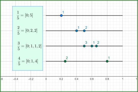
Figure 2.1. The “finite orbits” of $\frac{n}{5}$ for $n=1,2,3,4$ (GeoGebra [8]).

Since a single “$T$-orbit” of a rational number cannot converge to the Gauss measure $\nu_{\mathrm{Gauss}}$, we can hope that maybe a sequence of such orbits converge equidistribute:

Definition 3.

We say that a sequence $\mu_{i}$ of probability measures on $\left[0,1\right]$ equidistributes if $\mu_{i}\overset{w^{*}}{\longrightarrow}\nu_{\mathrm{Gauss}}$.

Problem 4.

Find $1\leq n_{m}\leq m$, $\left(n_{m},m\right)=1$ such that $\nu_{n_{m}/m}$ equidistributes, i.e. $\nu_{n_{m}/m}\overset{w^{*}}{\longrightarrow}\nu_{\mathrm{Gauss}}$ as $m\to\infty$.

Clearly, not every sequence $n_{m}$ defines an equidistributing sequence $\nu_{n_{m}/m}$. For example, as can be seen in 2.1, the measures $\nu_{1/m}=\delta_{1/m}$ are always Dirac measures on a single point, so that $\nu_{1/m}$ cannot converge to $\nu_{\mathrm{Gauss}}$. Similarly $\nu_{(m-1)/m}$ are supported on 2 points so they cannot equidistribute. But there are only 2 such “bad” measures for any $q$, and maybe the rest are not so bad.

With this in mind, for $m\in\mathbb{N}$ fixed we set $\Lambda_{m}=\left\{n\in\mathbb{N}\;\mid\;1\leq n\leq m,\;\left(n,m\right)=1\right\}$ and define the averages

$$\nu_{m}:=\frac{1}{\left|\Lambda_{m}\right|}{\displaystyle\sum_{n\in\Lambda_{m}}}\nu_{n/m}$$

where $\left|\Lambda_{m}\right|=\varphi\left(m\right)$ is the Euler totient function. Thus if the set of “bad” orbit measures is very small, they will not affect this average. In [2] the author and Uri Shapira proved that this is indeed the case, namely $\nu_{m}\overset{w^{*}}{\longrightarrow}\nu_{\mathrm{Gauss}}$.

It is interesting to ask what happens if we do not average over all of $\Lambda_{m}$, but only over, for example, half of it. If we decompose $\Lambda_{m}=\tilde{\Lambda}_{m}\sqcup\hat{\Lambda}_{m}$ to two halves, and let $\tilde{\nu}_{m},\hat{\nu}_{m}$ be the corresponding averages, then $\nu_{m}=\frac{1}{2}\tilde{\nu}_{m}+\frac{1}{2}\hat{\nu}_{m}$. We can now take the limit of both sides, where we might restrict to a subsequence to assume that $\tilde{\nu}_{m}$ and $\hat{\nu}_{m}$ converge to $\tilde{\nu}_{\infty}$ and $\hat{\nu}_{\infty}$ respectively to get the convex combination of

$$\nu_{\mathrm{Gauss}}=\frac{1}{2}\tilde{\nu}_{\infty}+\frac{1}{2}\hat{\nu}_{\infty}.$$

One of the defining properties of ergodic measures with respect to some action $T$ is that they are the extreme point in the space of $T$-invariant probability measure, namely they cannot be written as a nontrivial convex combination of $T$-invariant probability measures. It is not immediately clear that both $\tilde{\nu}_{\infty}$ and $\hat{\nu}_{\infty}$ are $T$-invariant, but this is true, and it will be much more obvious once we move on to the language of lattice and diagonal orbits. In any way, the property mentioned above, shows that both $\tilde{\nu}_{\infty}$ and $\hat{\nu}_{\infty}$ must be $\nu_{\mathrm{Gauss}}$. The constant $\frac{1}{2}$ was not really important , and we can actually do it for any $0<\alpha<1$.

This idea can be used to further upgraded the equidistribution result and show that the intuition about small “bad” sets is correct e there are families $\Lambda_{m}^{\prime}\subseteq\Lambda_{m}$ with $\frac{\left|\Lambda_{m}^{\prime}\right|}{\left|\Lambda_{m}\right|}\to 1$, such that for any choice of $n_{m}\in\mathcal{F}_{m}^{\prime}$ we have that $\nu_{n_{m}/m}\overset{w^{*}}{\longrightarrow}\nu_{Gauss}$ as $m\to\infty$. Thus in a philosophical sense we have a mean and a pointwise ergodic theorems for the rational (non generic) points as well.

Trying to prove this claim, leads to at least two problems that we must overcome.

• The standard dynamical method to solve such problems is to show that the limit measure $\nu_{m}\overset{w^{*}}{\longrightarrow}\nu_{\infty}$ (if it exists) is $T$-invariant, and then use some classification for $T$-invariant probability measure. If each of the $\nu_{m}$ were $T$-invariant in themselves, then clearly $\nu_{\infty}$ would be $T$-invariant as well. However, in our case not only are the measure not $T$-invariant, since $T\left(0\right)$ is not well defined, $T^{\ell}\left(\nu_{m}\right)$ is not well defined for any $\ell>1$.

• In the current formulation, each point the the orbits of $\frac{n}{m}$ for some $\left(n,m\right)=1$ has some positive weight in $\nu_{m}=\frac{1}{\varphi\left(m\right)}{\displaystyle\sum_{n\in\Lambda_{m}}}\nu_{n/m}$. However, its weight is determined according to which orbit it is in. For example, the “orbit” of $\frac{1}{5}$ contains only one point so its weight from there is $\frac{1}{1}\cdot\frac{1}{\varphi\left(5\right)}=\frac{1}{4}$. On the other hand, the “orbit” of $\frac{3}{5}$ has three points, so each point there contributes $\frac{1}{3}\cdot\frac{1}{\varphi\left(5\right)}=\frac{1}{12}$ mass to the measure $\nu_{m}$. If we want each such point to have the same measure, then we can define instead

  $$\tilde{\nu}_{m}=\frac{1}{\sum_{n\in\Lambda_{m}}\mathrm{len}\left(\frac{n}{m}\right)}\sum_{n\in\Lambda_{m}}\sum_{0}^{\mathrm{len}\left(\frac{n}{m}\right)-1}\delta_{T^{i}\left(\frac{n}{m}\right)},$$

  and similarly ask whether $\tilde{\nu}_{m}\to\nu_{\mathrm{Gauss}}$. Thus, in a sense it is not clear what is the “right” normalization. Interestingly, the upgrade mentioned above shows that both of these normalization equidistribute.

As we shall see, viewing this problem via the diagonal flow in the space of 2-dimensional unimodular lattices helps us solve both of these problems.

3. The continuous analogue and symmetries

It is well known that the continued fraction expansion of some $\alpha\in\left(0,1\right)$ can be extracted from a certain $A$-orbit in the space of 2-dimensional unimodular lattices $\mathrm{SL}_{2}\left(\mathbb{Z}\right)\backslash\mathrm{SL}_{2}\left(\mathbb{R}\right)$ where $A$ is the diagonal subgroup of $\mathrm{SL}_{2}\left(\mathbb{R}\right)$. Let us recall the main steps of this process.

For the rest of this section we fix the following notations:

$$X :=\mathrm{SL}_{2}\left(\mathbb{Z}\right)\backslash\mathrm{SL}_{2}\left(\mathbb{R}\right),\quad\mathbb{H}:=\mathrm{PSL}_{2}\left(\mathbb{R}\right)/\mathrm{PSO}_{2}\left(\mathbb{R}\right)$$

$$A :=\left\{a\left(t\right)=\left(\begin{array}[]{cc}e^{-t/2}&0\\ 0&e^{t/2}\end{array}\right)\;\mid\;t\in\mathbb{R}\right\}$$

$$U :=\left\{u_{x}=\left(\begin{array}[]{cc}1&x\\ 0&1\end{array}\right)\;\mid\;x\in\mathbb{R}\right\}$$

An element $\mathrm{SL}_{2}\left(\mathbb{Z}\right)\cdot g$ with $g\in\mathrm{SL}_{2}\left(\mathbb{R}\right)$ correspond to the lattice $\mathbb{Z}^{2}\cdot g$. To get some intuition we will look instead on the hyperbolic upper half plane $\mathbb{H}$ modulo the $\mathrm{SL}_{2}\left(\mathbb{Z}\right)$-action which we can actually draw. The fundamental domain for $\mathrm{SL}_{2}\left(\mathbb{Z}\right)$ in $\mathbb{H}$ is

$$\mathcal{F}=\left\{z\in\mathbb{C}\;\mid\;\left\|z\right\|>1,\;Im\left(z\right)>0,\;\left|Re\left(z\right)\right|<\frac{1}{2}\right\},$$

where a point $z\in\mathcal{F}$ correspond to the lattice $span_{\mathbb{Z}}\left(1,z\right)$.

Recall that $\mathrm{SL}_{2}\left(\mathbb{R}\right)$ act on the hyperbolic upper half plane $\mathbb{H}$ via the Möbius transformation ${\scriptstyle\left(\begin{array}[]{cc}a&b\\ c&d\end{array}\right)}z=\frac{az+b}{cz+d}$. The geodesics in $\mathbb{H}$ are $gAi,\;g\in\mathrm{SL}_{2}\left(\mathbb{R}\right)$, which in $\mathbb{H}$ look like either half circles with their ends on the $x$-axis, or vertical lines. Trying to compute the endpoints, namely the limit when $t\to\pm\infty$ we get that

$$\left(\begin{array}[]{cc}a&b\\ c&d\end{array}\right)a\left(t\right)i=\frac{ae^{-t}i+b}{ce^{-t}i+d}=\begin{cases}\frac{a}{c}&t\to-\infty\\ \frac{b}{d}&t\to\infty\end{cases}.$$

In particular for $g=u_{\alpha},\;\alpha\in\mathbb{R}$, the endpoint of $u_{\alpha}a\left(t\right)i$ in the past is $\frac{1}{0}=\infty$, while in the future it is $\alpha$, so that the geodesic $u_{\alpha}Ai$ is the line $x=\alpha$. We then consider the projection of this geodesic to the modular surface $\mathrm{SL}_{2}\left(\mathbb{Z}\right)\backslash\mathbb{H}\cong\mathrm{PSL}_{2}\left(\mathbb{Z}\right)\backslash\mathrm{PSL}_{2}\left(\mathbb{R}\right)/\mathrm{SO}_{2}\left(\mathbb{R}\right)$, or equivalently to the standard fundamental domain $\mathcal{F}$.

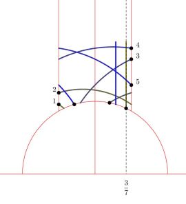
Figure 3.1. The geodesic from $\infty$ to $\frac{3}{7}$ projected to $\mathrm{SL}_{2}\left(\mathbb{Z}\right)\backslash\mathbb{H}$: Coming from the cusp, it first hits the bottom, then 2-times the left boundary, the bottom again, 3-times the right boundary, the bottom, and then go straight up to the cusp. These boundary hitting can be seen in the continued fraction expansion of $\frac{3}{7}$ which is $\frac{3}{7}=\frac{1}{2+\frac{1}{3}}=\left[0;2,3\right]$.

Every time the geodesic leaves the fundamental domain $\mathcal{F}$, we need to act with a matrix in $\mathrm{SL}_{2}\left(\mathbb{Z}\right)$ in order to bring it back inside. In particular, the matrices corresponding to the left and right boundary of $\mathcal{F}$ are ${\scriptstyle\left(\begin{array}[]{cc}1&1\\ 0&1\end{array}\right)},{\scriptstyle\left(\begin{array}[]{cc}1&-1\\ 0&1\end{array}\right)}$, and to the lower boundary we have the matrix ${\scriptstyle\left(\begin{array}[]{cc}0&1\\ -1&0\end{array}\right)}$. These transformations affect the endpoints of the geodesic via the maps $x\mapsto x\pm 1$ and $x\mapsto-\frac{1}{x}$. Note that this is more or less what we use in the Gauss map $T\left(x\right)=\frac{1}{x}-\left\lfloor\frac{1}{x}\right\rfloor$ e indeed, we first apply $x\mapsto\frac{1}{x}$, and then decrease by $-1$ exactly $\left\lfloor\frac{1}{x}\right\rfloor$ times. Geometrically, the geodesic hits the lower boundary and then (more or less) $\left\lfloor\frac{1}{x}\right\rfloor$ times the right boundary before coming back to the lower boundary. The minus sign in the action ${\scriptstyle\left(\begin{array}[]{cc}0&1\\ -1&0\end{array}\right)}\left(x\right)=-\frac{1}{x}$ above produce an alternation between the left and right boundary. As can be seen in the example in 3.1, the geodesic from $\infty$ to $\frac{3}{7}$ hits two times the left boundary and then 3 times the right boundary, and the corresponding CFE of $\frac{3}{7}$ is $\frac{3}{7}=\left[0;2,3\right]$. For the exact connection between the continued fraction expansion and the diagonal flow in $\mathrm{SL}_{2}\left(\mathbb{Z}\right)\backslash\mathrm{SL}_{2}\left(\mathbb{R}\right)$, we refer the reader to section 9.6 in [6].

The spaces $X=\mathrm{SL}_{2}\left(\mathbb{Z}\right)\backslash\mathrm{SL}_{2}\left(\mathbb{R}\right)$ and $\mathrm{SL}_{2}\left(\mathbb{Z}\right)\backslash\mathbb{H}\cong X_{2}/\mathrm{SO}_{2}\left(\mathbb{R}\right)$ are quite similar since $\mathrm{SO}_{2}\left(\mathbb{R}\right)$ is a compact group, so the picture above gives a very good intuition of what happens in $X$. For example, an important phenomenon for $A$-orbits of the form $\mathrm{SL}_{2}\left(\mathbb{Z}\right)u_{\alpha}A$ in $X$ with rational $\alpha\in\mathbb{Q}$, as can be seen in 3.1, is that they come and eventually return to the cusp, and we call such orbits divergent. Indeed, this follows from the fact that under the $\mathrm{SL}_{2}\left(\mathbb{Z}\right)$-Möbius action, all the rational points and $\infty$ are equivalent. This is the analogue of the fact that continued fraction expansion of rationals are finite (or equivalently $T^{k}\left(\frac{n}{m}\right)=0$ for some $k$). We can always define the $A$-invariant measure on the orbit $\mathrm{SL}_{2}\left(\mathbb{Z}\right)gA$ by pushing the standard Lebesgue measure from $stab\left(\mathrm{SL}_{2}\left(\mathbb{Z}\right)g\right)\backslash A$. Unless the orbit is periodic, or equivalently $stab\left(\mathrm{SL}_{2}\left(\mathbb{Z}\right)g\right)$ is a lattice in $A\cong\mathbb{R}$, then the measure is infinite. However for divergent orbits this measure is locally finite - the measure of any compact set is finite (because most of the mass of the measure is near the cusp).

Let us denote by $\mu_{n/m}$ this $A$-invariant measure on the orbit $\mathrm{SL}_{2}\left(\mathbb{Z}\right)u_{n/m}A$ and define $\mu_{m}=\frac{1}{\left|\Lambda_{m}\right|}\sum_{n\in\Lambda_{m}}\mu_{n/m}$. The analogue of the equidistribution $\nu_{m}\overset{w^{*}}{\longrightarrow}\nu_{\mathrm{Gauss}}$ in the continued fraction setting is $\mu_{m}\to\mu_{Haar}$, where $\mu_{Haar}$ is the $\mathrm{SL}_{2}\left(\mathbb{R}\right)$-invariant measure on $X=\mathrm{SL}_{2}\left(\mathbb{Z}\right)\backslash\mathrm{SL}_{2}\left(\mathbb{R}\right)$. Note that since $\mu_{m}$ are only locally finite, and not probability measure, by the limit we mean that $\frac{\mu_{m}\left(f_{1}\right)}{\mu_{m}\left(f_{2}\right)}\overset{q\to\infty}{\to}\frac{\mu_{Haar}\left(f_{1}\right)}{\mu_{Haar}\left(f_{2}\right)}$ for any $f_{1},f_{2}\in C_{c}\left(X\right)$ with $\mu_{Haar}\left(f_{2}\right)\neq 0$ (see 9.1 for more details about locally finite measures and their limits).

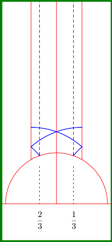
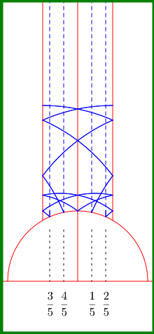
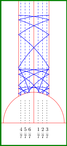
Figure 3.2. From left to right we have the $A$-orbits on which $\mu_{3},\mu_{5}$ and $\mu_{7}$ are supported.

There are three main advantages of working with $X$ instead of with continued fractions, which can already be seen in the examples in 3.2:

1. Unlike the measures $\nu_{m}$ on which we cannot really act with the Gauss map $T$, the measures $\mu_{m}$ are $A$-invariant. Of course we didn’t get this for free e we now work with infinite locally finite measures instead of probability measure. Fortunately, most of the mass of these measures are near the cusp, so as we shall see later, we can reduce this problem to finite measures. Also, we will soon see that the time the $A$-orbit-measure $\mu_{n/m}$ spends in $X$ “before” diverging to the cusp (minus their “vertical” parts) doesn’t depend on $n$. Thus, unlike the continued fraction result where we had two type of averages in $\nu_{n}$ and $\tilde{\nu}_{n}$, in this setting we have only one natural way to average.

2. The pictures are symmetric with respect to the $y$-axis. Moreover, we know that the $A$-orbits leading to rational numbers come and go to the cusp, but instead of having two vertical lines for each orbit, to a total of $2\varphi\left(m\right)$, we only have $\varphi\left(m\right)$. In other words, a geodesic leading to $\frac{n}{m}$, will eventually go straight to the cusp, but the corresponding vertical line will be over $\frac{n^{\prime}}{m}$ for some $n^{\prime}$. This symmetry can be expressed in the continued fraction form, but cannot seen as clearly as in 3.2.

3. If we don’t fold the orbits into the fundamental domain, and only consider their vertical geodesics, then all of these are parallel lines which we can get one from the other by translation in the $x$-coordinate. This almost correspond to the unipotent flow in $X$ and in general unipotent flows are much better understood than geodesic flows.

These phenomena are key to proving the equidistribution result.

4. Symmetries and hidden horospheres

Part (3) above is probably one of the most important observations, since it allow us to use horocycles and not just geodesics.

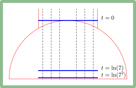
Figure 4.1. The dashed lines are the geodesics without foldings modulo $\mathrm{SL}_{2}\left(\mathbb{Z}\right)$. The blue segments are horocycles e at time $t$ it is in the Euclidean height $e^{-t}$.

For every $h$, the horocycle at height $h$ (blue lines in 4.1) contains $\varphi\left(m\right)$ points, one from each geodesic. Let us assume that as $m\to\infty$, in every height $h$ taking the uniform average over the $\varphi\left(m\right)$ points is more or less the uniform measure over the whole horocycle. Our measure is the average over $\varphi\left(m\right)$ orbits of the diagonal group $A$, and switching the order of integration we can first take the discrete average in each height, and then take their averages along the $A$ direction. With our assumption above, this will be more or less the same as taking the uniform average in each horocycle, and then taking the averages of the horocycles.

We now have one of the main results in this space, namely the fact that expanding horocycles equidistribute: if we take a single horocycle, e.g. at height $t=0$, and push it by a diagonal element $a\in A$ which expands it (in the picture, this means pushing it down), then as $a$ increases to infinity the pushed horocycles equidistribute inside the whole space. More formally:

Definition 5 (Uniform measure on the standard horocycle).

Let $\mu_{U}$ be the pushforward of the Lebesgue measure on $\left[0,1\right]$ to $x\mapsto\mathrm{SL}_{2}\left(\mathbb{Z}\right)u_{x}$, namely $\mu_{U}\left(f\right):=\int_{0}^{1}f\left(\mathrm{SL}_{2}\left(\mathbb{Z}\right)u_{x}\right)\mathrm{dx}$ for $f\in C_{c}\left(X_{2}\right)$.

Theorem 6.

Expanding horocycles equidistribute e i.e. $a\left(-t\right)_{*}\mu_{U}\overset{w^{*}}{\longrightarrow}\mu_{Haar}$ as $t\to\infty$.

This result explains why we expect our measures $\mu_{m}$ to equidistribute in $X$ (or at least their part with $t\geq 0$, though as we shall see, this will be enough). Hence, we only need to justify our assumption that the discrete average over the $\varphi\left(m\right)$ points is almost the uniform measure over the corresponding horocycle.

For that, first note that the horocycle at height $1=e^{-0}$ is just $\left\{\mathrm{SL}_{2}\left(\mathbb{Z}\right)\cdot u_{x}\;\mid\;x\in\mathbb{R}\right\}$, and since $u_{1}={\scriptstyle\left(\begin{array}[]{cc}1&1\\ 0&1\end{array}\right)}\in\mathrm{SL}_{2}\left(\mathbb{Z}\right)$, the horocycle is homeomorphic to a cycle $\nicefrac{{\mathbb{R}}}{{\mathbb{Z}}}$. Under this identification, the $\varphi\left(m\right)$ points on it are simply $\frac{1}{m}\Lambda_{m}=\left\{\frac{n}{m}\;\mid\;1\leq n\leq m,\;\left(n,m\right)=1\right\}$.

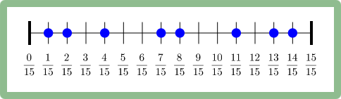
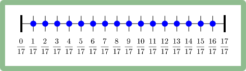
Figure 4.2. The sets $\frac{1}{15}\Lambda_{15}$ and $\frac{1}{17}\Lambda_{17}$ inside the segment $\left[0,1\right]$. The missing points on the left correspond to numbers divisable by $3$ and $5$.

As can be seen for example in the figure above for $m=17$, for primes $m$ the sets $\frac{1}{m}\Lambda_{m}$ equidistribute in $\left[0,1\right]$ as $m\to\infty$. If $m$ is not prime, then we get “holes” in $\left[0,1\right]$ for each $n$ not coprime to $m$, and there are more and more holes the more prime divisors $m$ has. However, as we shall see later (62) using a simple inclusion exclusion argument, even in these cases the $\varphi\left(m\right)$ points equidistribute in $\left[0,1\right]$.

We can do the same for other horocycles in different heights, but the argument above is not enough. While all the horocycles are homeomorphic to cycles, the length of the cycle is not fixed. The lower we are in 4.1 the larger the cycle is in the hyperbolic plane (the distance between the vertical lines increase). In particular, there is a point where the horocycle is isometric to $\nicefrac{{\left[0,m\right]}}{{0\sim m}}$ and the points are simply the integers $n$ with $\left(n,m\right)=1$ so they are at least at distance 1 from each other. The average over these points and the uniform measure on $\left[0,m\right]$ are quite far away.

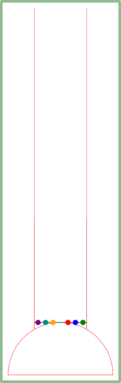
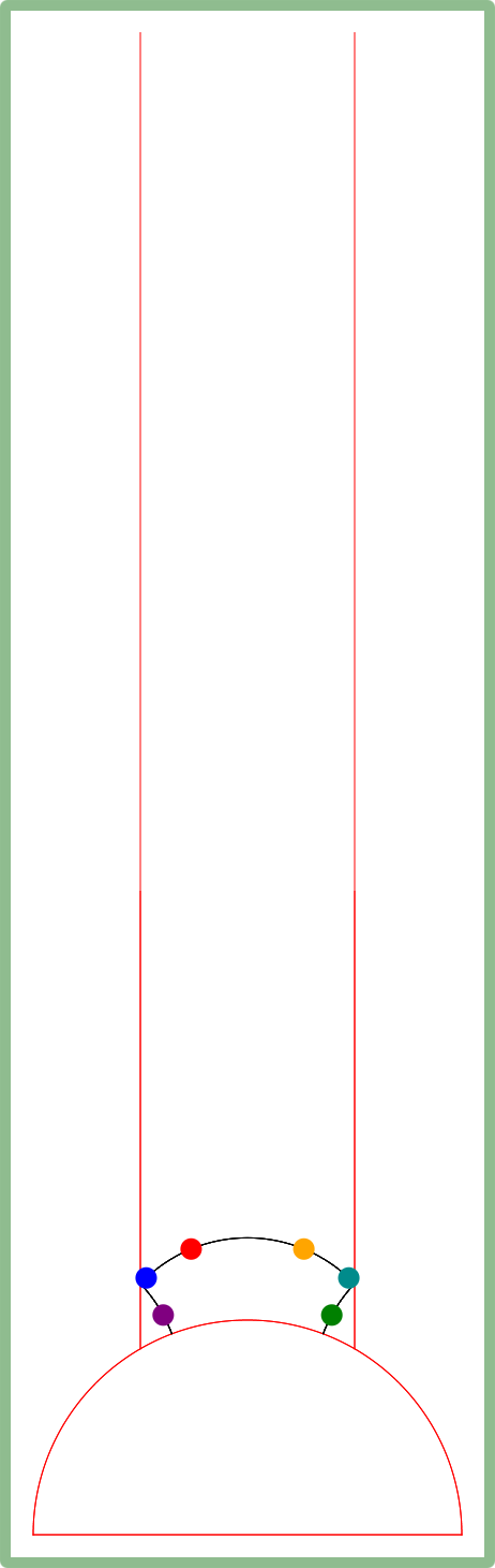
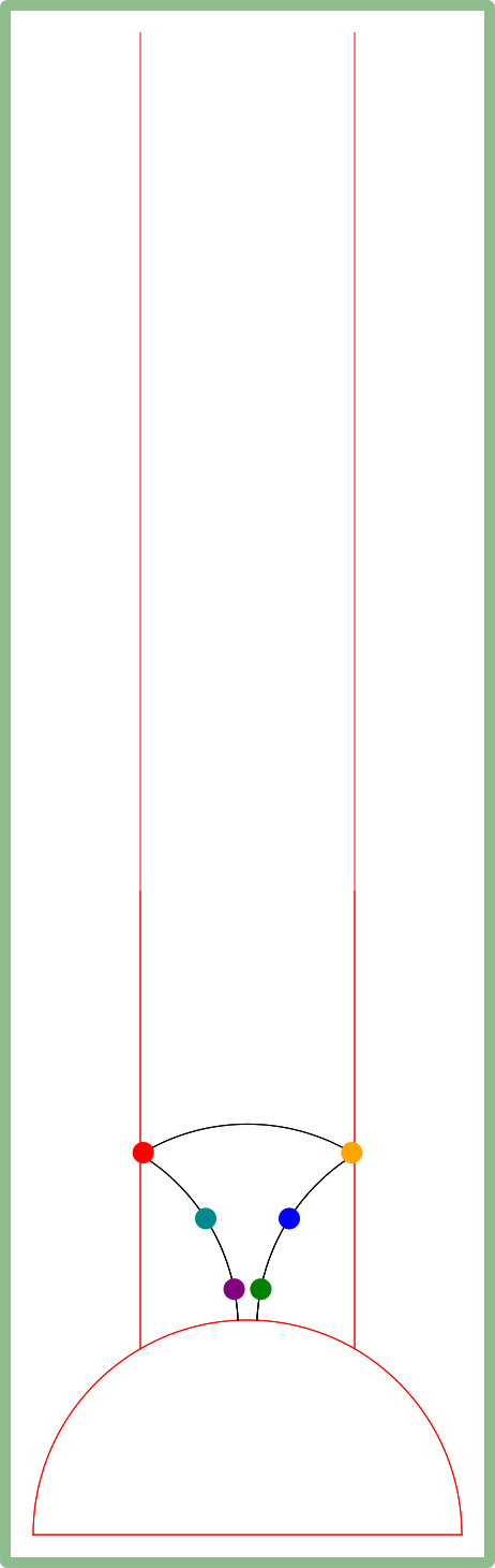
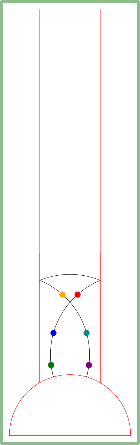
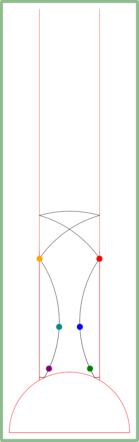
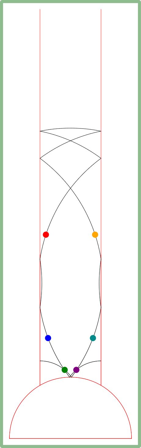
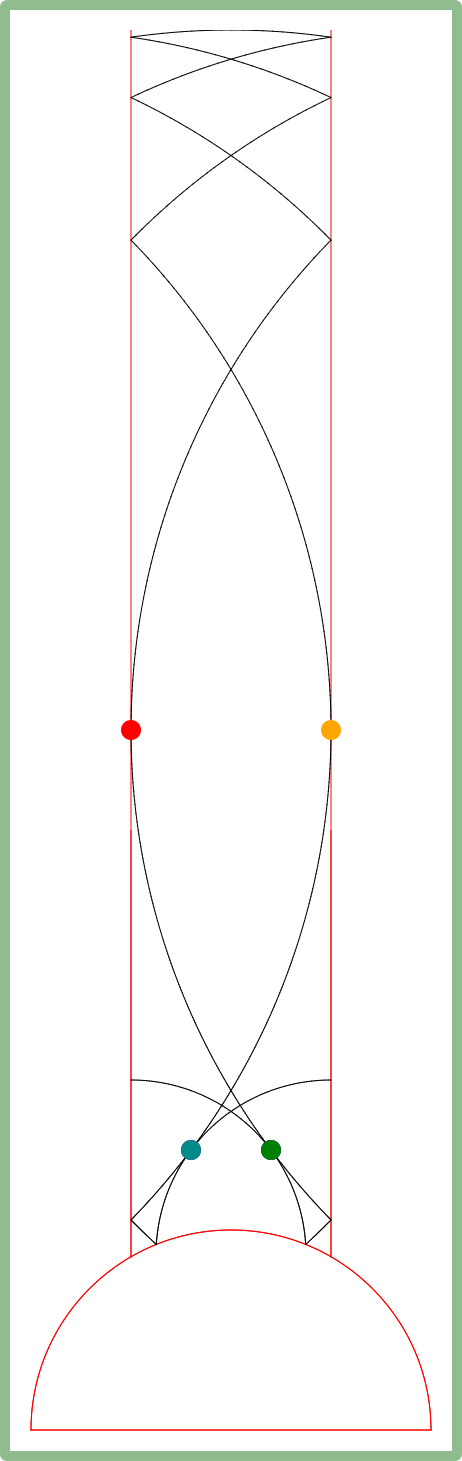
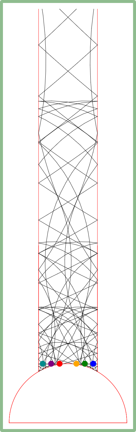
Figure 4.3. For $m=7$, in the first 7 images from the left we see the $\varphi\left(7\right)$ points on the corresponding horocycle at times $t=\ln\left(7\right)\cdot\frac{i}{6},\;i=0,1,...,6$. The right most image is at time $t=2\cdot\ln\left(7\right)$.

As can be seen in the image above, at time $0$ our points are very close to one another along the horocycle. As $t$ increases this distance becomes longer and longer until at time $t=\ln\left(7\right)$ they are quite far away. While the distance along the horocycle continues to grow, when we get to time $2\ln\left(7\right)$ all the points return to the same horocycle. If we ignore the horocycle itself, then the pictures at time $t=0$ and $t=2\ln\left(7\right)$ are exactly the same. This is part of a symmetry that we will use later on which shows that the time $\left[\ln\left(m\right),2\ln\left(m\right)\right]$ are a mirror image of the times $\left[0,\ln\left(m\right)\right]$.

To understand this expanding problem formally we do the following simple computation:

$$\mathrm{SL}_{2}\left(\mathbb{Z}\right)u_{\left(n+1\right)/m}a\left(t\right)=\mathrm{SL}_{2}\left(\mathbb{Z}\right)u_{n/m}a\left(t\right)a\left(-t\right)u_{1/m}a\left(t\right)=\mathrm{SL}_{2}\left(\mathbb{Z}\right)u_{n/m}a\left(t\right)\cdot u_{e^{t}/m}.$$

This tells us that at time $t$, the distance (over the horocycle) between the points corresponding to $\frac{n}{m}$ and $\frac{n+1}{m}$ is $\frac{e^{t}}{m}$. Hence, as long as $\frac{e^{t}}{m}$ is small, say $t\leq\left(1-\varepsilon\right)\ln\left(m\right)$ for some fixed $\varepsilon>0$, the argument that the discrete average is closed to the uniform average over the horocycle works.

As $t\geq\ln\left(m\right)$ grows, the distance between consecutive points increases to infinity (along the horocycle), however luckily for us our orbits have a nice algebraic structure which we can exploit. There is a symmetry at the time $\leq\ln\left(m\right)$ and at the times $\geq\ln\left(m\right)$ which we just saw an example in 4.3

Let us make this notion more precise.

Recall that the point $\mathrm{SL}_{2}\left(\mathbb{Z}\right)g\in X$ correspond to the lattice $\mathbb{Z}^{2}\cdot g\subseteq\mathbb{R}^{2}$, and in particular we have that $\mathbb{Z}^{2}u_{\alpha}=span_{\mathbb{Z}}\left\{\left(0,1\right),\left(1,\alpha\right)\right\}$. Let $1\leq n\leq m,\;\left(n,m\right)=1$ and consider the lattices

$$L_{n/m} =\mathbb{Z}^{2}u_{\alpha}=span_{\mathbb{Z}}\left\{\left(0,1\right),\left(1,\frac{n}{m}\right)\right\}$$

$$L_{m} =\mathbb{Z}^{2}\left(\begin{array}[]{cc}m&0\\ 0&1\end{array}\right)=span_{\mathbb{Z}}\left\{\left(0,1\right),\left(m,0\right)\right\}.$$

Note that $\left(m,0\right)=m\left(1,\frac{n}{m}\right)-n\left(0,1\right)$ is in $L_{n/m}$ so that $L_{m}$ is a sublattice of $L_{n/m}$. Furthermore $covol\left(L_{m}\right)=m$ and $\nicefrac{{L_{n/m}}}{{L_{m}}}\cong\nicefrac{{\mathbb{Z}}}{{m\mathbb{Z}}}$ (because $\left(n,m\right)=1$). As example, see the left picture in 4.4 below.

If $L\leq\mathbb{R}^{2}$ is any lattice which contains $L_{m}$ such that $\nicefrac{{L}}{{L_{m}}}=\nicefrac{{\mathbb{Z}}}{{m\mathbb{Z}}}$ then $L_{m}\leq L\leq\frac{1}{m}L_{m}$ and $\nicefrac{{\frac{1}{m}L_{m}}}{{L}}\cong\nicefrac{{\mathbb{Z}}}{{m\mathbb{Z}}}$ as well. It is now a standard argument to show that $L$ must be $L_{n/m}$ for some $\left(n,m\right)=1$. This already gives us a good starting point e these $L_{n/m}$ are exactly the representatives of the distinct $A$-orbits, and this point of view group them naturally together as certain lattices which contain $L_{m}$.

The lattice $L_{n/m}$ all lie on the horocycle of height $t=0$. As we want to check what happens at general time $t$, we simply multiply by $a\left(t\right)$. In particular at time $t=\ln\left(m\right)$, that we already encountered above, something interesting happens to $L_{m}$. Indeed, we get

$$L_{m}a\left(\ln\left(m\right)\right)=\mathbb{Z}^{2}\left(\begin{array}[]{cc}m&0\\ 0&1\end{array}\right)\left(\begin{array}[]{cc}m^{-1/2}&0\\ 0&m^{1/2}\end{array}\right)=m^{1/2}\mathbb{Z}^{2}$$

which is just a stretching of the lattice $\mathbb{Z}^{2}$, and in particular it is invariant under the reflection of switching the $x$ and $y$ coordinates. Let us denote this reflection by $\tau$, namely $\tau\left(x,y\right)=\left(y,x\right)$, so that $\tau\left(L_{m}a\left(\ln\left(m\right)\right)\right)=L_{m}a\left(\ln\left(m\right)\right)$. It is also easy to check that $L_{m}a\left(2\ln\left(m\right)\right)=\tau\left(L_{m}\right)$.

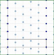
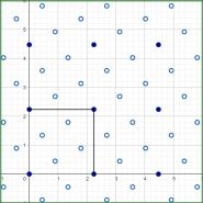
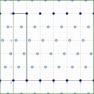
Figure 4.4. From left to right are the lattices $L_{3/5}a\left(t\right)$ (circles) and $L_{5}a\left(t\right)$ (full balls) at times $t=i\cdot\ln\left(5\right),\;i=0,1,2$ (GeoGebra [8]).

As can be seen in 4.4, unlike $L_{m}a\left(\ln\left(m\right)\right)$ in the middle picture, the lattice $L_{n/m}a\left(\ln\left(m\right)\right)$ is not invariant under the reflection $x\leftrightarrow y$. Its reflection, however, looks similar to $L_{n/m}a\left(\ln\left(m\right)\right)$ e both contain $\sqrt{m}\mathbb{Z}^{2}$ as a sublattice, and the quotient is $\nicefrac{{\mathbb{Z}}}{{m\mathbb{Z}}}$. Hence $\tau\left(L_{n/m}a\left(\ln\left(m\right)\right)\right)=L_{n^{\prime}/m}a\left(\ln\left(m\right)\right)$ for some $n^{\prime}$ coprime to $m$, and a simple computation shows that $nn^{\prime}\equiv_{m}-1$. So while the lattice itself is not invariant under this reflection, the set $\left\{L_{n/m}a\left(\ln\left(m\right)\right)\;\mid\;n\in\Lambda_{m}\right\}$ is invariant. We can do the same argument for the left and right images in 4.4 which are almost reflections of one another. So up to changing the $n$ with $n^{\prime}$, going forward from time $t=\ln\left(m\right)$ and going backwards are the same up to this reflection. More formally, we have that

$$\tau\left(L_{n/m}a\left(\ln\left(m\right)+t\right)\right)=L_{n^{\prime}/m}a\left(\ln\left(m\right)-t\right).$$

Because we want to take the average over all the $n$, we get that the average at time $\ln\left(m\right)+t$ is the same as the average at time $\ln\left(m\right)-t$ composed with the reflection. Thus, if we can show that our measures equidistribute at the times $t\leq\ln\left(m\right)$, then this reflection implies that they also equidistribute at times $t\geq\ln\left(m\right)$. With this in mind, we decompose our orbits to 4 parts (which in 4.1 are separated by the blue lines):

1. $t<0$: The orbit come from the cusp directly to the horocycle $\left\{\mathrm{SL}_{2}\left(\mathbb{Z}\right)u_{x}\;\mid\;0\leq x\leq 1\right\}$. Most of the mass here is near the cusp, so in any way it will not contribute too much to our measure.

2. $0<t<\ln\left(m\right)$: The orbit flows from the standard horocycle above up to a $\tau$-invariant set. In these times the discrete points equidistribute along their corresponding horocycle (up to some small distance from $\ln\left(m\right)$) and further more, the horocycles are expanding and therefore they equidistribute in the whole space.

3. $\ln\left(m\right)<t<2\ln\left(m\right)$: The mirror image of $0<t<\ln\left(m\right)$.

4. $2\ln\left(m\right)<t$: The mirror image of $t<0$ e the orbits starts at the transposed horocycle $\left\{\mathrm{SL}_{2}\left(\mathbb{Z}\right)u_{x}^{T}\;\mid\;0\leq x\leq 1\right\}$ and flow directly to the cusp.

Thus, in the end, it is enough to show that our equidistribution argument works at the times $0<t<\ln\left(m\right)$, and we already have a good reason for that to hold.

5. The $p$-adic motivation

Using the process and language described in the previous section, one can already prove full equidistribution. However, this result becomes much more natural once we begin to use the language of $p$-adic and adelic numbers. For example, on each horocycle we only have a finite set of points which only approximate the horocycle. There are many families of points which can do that, so what natural reason do we have to choose these exact families, and why do they all fit together so nicely? If we ever try to generalize this equidistribution result to higher dimension, which families would we want to choose then? The language of adelic numbers make this discussion much more natural and even answer some of these questions.

Recall that our measure $\mu_{m}$ as viewed in the hyperbolic plane looks like $\varphi\left(m\right)$ vertical lines (see 4.1), in particular we can think of it as a single line translated by matrices of the form $u_{x}$ from the left. However, our whole discussion is in the modular surface $\mathrm{SL}_{2}\left(\mathbb{Z}\right)\backslash\mathrm{SL}_{2}\left(\mathbb{R}\right)$, so this left translation is not well defined. In order to make this process well defined, we need to go to a bigger space which projects onto the space of unimodular lattices.

At time $t$, our $\varphi\left(m\right)$ points are $\mathrm{SL}_{2}\left(\mathbb{Z}\right)u_{n/m}a\left(t\right)$ with $1\leq n\leq m,\;\left(n,m\right)=1$. Thus, in a sense we want to take $\mathrm{SL}_{2}\left(\mathbb{Z}\right)a\left(t\right)$ and “multiply” if from the right by $u_{n/m}$ with $n\in\Lambda_{m}$. The matrices $u_{n/m}$ are all in $\mathrm{SL}_{2}\left(\mathbb{Z}\left[\frac{1}{m}\right]\right)$, which suggests that we might want to work with the space $\mathrm{SL}_{2}\left(\mathbb{Z}\left[\frac{1}{m}\right]\right)\backslash\mathrm{SL}_{2}\left(\mathbb{R}\right)$ instead. However, in this space the points $\mathrm{SL}_{2}\left(\mathbb{Z}\left[\frac{1}{m}\right]\right)u_{n/m}a\left(t\right),\;n\in\Lambda_{m}$ are identified to a single point, which is not what we wanted, and even without this problem, the group $\mathrm{SL}_{2}\left(\mathbb{Z}\left[\frac{1}{m}\right]\right)$ is not a lattice in $\mathrm{SL}_{2}\left(\mathbb{R}\right)$ so we cannot use all the results about lattices. Fortunately, there is an easy and natural way to solve it e we look instead on the diagonal embedding $\mathrm{SL}_{2}\left(\mathbb{Z}\left[\frac{1}{m}\right]\right)\hookrightarrow\mathrm{SL}_{2}\left(\mathbb{R}\right)\times\mathrm{SL}_{2}\left(\mathbb{Z}\left[\frac{1}{m}\right]\right)$ and the quotient space

$$\mathrm{SL}_{2}\left(\mathbb{Z}\left[\frac{1}{m}\right]\right)\backslash\mathrm{SL}_{2}\left(\mathbb{R}\right)\times\mathrm{SL}_{2}\left(\mathbb{Z}\left[\frac{1}{m}\right]\right).$$

By definition, every pair $\left(g^{\left(\infty\right)},g^{\left(m\right)}\right)\in\mathrm{SL}_{2}\left(\mathbb{R}\right)\times\mathrm{SL}_{2}\left(\mathbb{Z}\left[\frac{1}{m}\right]\right)$ is equivalent to $\left(\left(g^{\left(m\right)}\right)^{-1}g_{\infty},Id\right)$, and it is easy to check that the map

$$\pi_{m}:\mathrm{SL}_{2}\left(\mathbb{Z}\left[\frac{1}{m}\right]\right)\left(g^{\left(\infty\right)},g^{\left(m\right)}\right)\mapsto\mathrm{SL}_{2}\left(\mathbb{Z}\right)\left(g^{\left(m\right)}\right)^{-1}g_{\infty}\in\mathrm{SL}_{2}\left(\mathbb{Z}\right)\backslash\mathrm{SL}_{2}\left(\mathbb{R}\right),$$

is a well defined surjective map. It is also not hard to show that the preimage of $\mathrm{SL}_{2}\left(\mathbb{Z}\right)g^{\left(\infty\right)}$ is exactly the orbit $\mathrm{SL}_{2}\left(\mathbb{Z}\left[\frac{1}{m}\right]\right)\left(g^{\left(\infty\right)},\mathrm{SL}_{2}\left(\mathbb{Z}\right)\right)$. In particular, the projection $\pi_{m}$ induces an isomorphism

$$\mathrm{SL}_{2}\left(\mathbb{Z}\left[\frac{1}{m}\right]\right)\backslash\left[\mathrm{SL}_{2}\left(\mathbb{R}\right)\times\mathrm{SL}_{2}\left(\mathbb{Z}\left[\frac{1}{m}\right]\right)\right]/\left[Id\times\mathrm{SL}_{2}\left(\mathbb{Z}\right)\right]\cong\mathrm{SL}_{2}\left(\mathbb{Z}\right)\backslash\mathrm{SL}_{2}\left(\mathbb{R}\right).$$

Philosophically, this new presentation of the space of lattices tell us that these is a right “action” of $\mathrm{SL}_{2}\left(\mathbb{Z}\left[\frac{1}{m}\right]\right)/\mathrm{SL}_{2}\left(\mathbb{Z}\right)$ on our standard space of unimodular lattices $\mathrm{SL}_{2}\left(\mathbb{Z}\right)\backslash\mathrm{SL}_{2}\left(\mathbb{R}\right)$.

For example, our set $\mathrm{SL}_{2}\left(\mathbb{Z}\right)u_{n/m}a\left(t\right),\;n\in\Lambda_{m}$ from before can now be seen as the projection of

$$\left\{\mathrm{SL}_{2}\left(\mathbb{Z}\left[\frac{1}{m}\right]\right)\left(a\left(t\right),u_{-n/m}\right),\;n\in\Lambda_{m}\right\}=\mathrm{SL}_{2}\left(\mathbb{Z}\left[\frac{1}{m}\right]\right)\left(a\left(t\right),Id\right)\cdot\left\{\left(Id,u_{-n/m}\right),\;n\in\Lambda_{m}\right\},$$

namely it is a projection of an orbit of the set $\left\{\left(Id,u_{-n/m}\right),\;n\in\Lambda_{m}\right\}$. Note that the map $x\mapsto u_{x}$ from $\mathbb{R}$ to $U$ is an isomorphism so we can identify $\left\{\left(Id,u_{-n/m}\right),\;n\in\Lambda_{m}\right\}$ with $\frac{1}{m}\Lambda_{m}$. Since we only care about the projection of this orbit, and the projection is constant on $Id\times\mathrm{SL}_{2}\left(\mathbb{Z}\right)$ which contains $\left(Id,u_{1}\right)$, we can actually think of this set as $\frac{1}{m}\Lambda_{m}\;(mod\;1)$ or $\Lambda_{m}\;(mod\;m)$.

This is already a better presentation, since now we have an actual orbit. Unfortunately, the matrix multiplication of the $u_{x}$ translate to addition of $x$, and even when considered mod $m$, the set $\Lambda_{m}$ is not of a group (additively). However, it is a group multiplicatively, and we want to somehow exploit this fact.

In order to present this as a group action we first write the $u_{n/m}$ as conjugations

$$u_{n/m}=\left(\begin{array}[]{cc}1&0\\ 0&n^{-1}\end{array}\right)u_{-1/m}\left(\begin{array}[]{cc}1&0\\ 0&n\end{array}\right).$$

The set $\left\{\left(\begin{array}[]{cc}1&0\\ 0&n^{-1}\end{array}\right)\;\mid\;n\in\Lambda_{m}\right\}$ is again not a group, but unlike before, when we consider the multiplication mod $m$ it is a group.

Both the problem that our new set is only a group mod $m$, and that the matrices ${\scriptstyle\left(\begin{array}[]{cc}1&0\\ 0&n^{-1}\end{array}\right)}$ are not in $\mathrm{SL}_{2}\left(\mathbb{Z}\left[\frac{1}{m}\right]\right)$ (the determinant is not in $\mathbb{Z}\left[\frac{1}{m}\right]^{\times}$) can be fixed once we move to the groups $\mathrm{GL}_{2}\left(\mathbb{Q}_{m}\right)$ and $\mathrm{GL}_{2}\left(\mathbb{Z}_{m}\right)$ instead of $\mathrm{SL}_{2}\left(\mathbb{Z}\left[\frac{1}{m}\right]\right)$ and $\mathrm{SL}_{2}\left(\mathbb{Z}\right)$ in the right coordinate of our bigger space.

There are many ways to define the $m$-adic integers $\mathbb{Z}_{m}$ and $m$-adic numbers $\mathbb{Q}_{m}$, and we refer the reader to [7, 9] for further details. Probably the most elementary way is as rings of formal power series where

$$\mathbb{Z}_{m} =\left\{\sum_{0}^{\infty}a_{j}m^{j}\;\mid\;a_{j}\in\left\{0,...,m-1\right\}\right\}.$$

$$\mathbb{Q}_{m} =\left\{\sum_{N}^{\infty}a_{j}m^{j}\;\mid\;N\in\mathbb{Z},\;a_{j}\in\left\{0,...,m-1\right\}\right\}$$

The first important observation is that the map $\rho\left(\sum_{0}^{\infty}a_{j}m^{j}\right)=a_{0}\;(mod\;m)$ from $\mathbb{Z}_{m}$ to $\nicefrac{{\mathbb{Z}}}{{m\mathbb{Z}}}$ is a well defined homomorphism of rings. There are many results which we can get from this homomorphism into the finite ring $\nicefrac{{\mathbb{Z}}}{{m\mathbb{Z}}}$ (and the similarly defined homomorphism into the rings $\nicefrac{{\mathbb{Z}}}{{m^{k}\mathbb{Z}}}$). This homomorphisms are at the core of these $m$-adic numbers and we will use them repeatedly. As a first example, we use it to study the invertible elements and the general structure of $\mathbb{Z}_{m}$ and $\mathbb{Q}_{m}$.

Claim 7.

An element $z=\sum_{0}^{\infty}a_{j}m^{j}\in\mathbb{Z}_{m}^{\times}$ is invertible if and only if $\left(a_{0},m\right)=1$ or equivalently $\rho\left(z\right)\in\left(\nicefrac{{\mathbb{Z}}}{{m\mathbb{Z}}}\right)^{\times}$.

Proof.

Let $\sum_{0}^{\infty}b_{j}m^{j}\in\mathbb{Z}_{m}$ and write

$$\left(\sum_{0}^{\infty}a_{j}m^{j}\right)\left(\sum_{0}^{\infty}b_{j}m^{j}\right)=\left(\sum_{0}^{\infty}c_{j}m^{j}\right).$$

The fact that $\rho$ is homomorphism implies in particular that $a_{0}b_{0}\equiv_{m}c_{0}$. It follows that if $\sum_{0}^{\infty}a_{j}m^{j}\in\mathbb{Z}_{m}^{\times}$, then $a_{0}$ is invertible mod $m$, namely $\left(a_{0},m\right)=1$. For the other direction, a simple induction argument shows that we can always choose $b_{j}$ so that $c_{0}=1$ and $c_{j}=0$ for all $n\geq 1$.

∎

Corollary 8.

The following holds:

1. We can write $\mathbb{Z}_{m}^{\times}=\bigcup_{n}\left(n+m\mathbb{Z}_{m}\right)$ where $n\in\Lambda_{m}$.

2. We have that $\mathbb{Z}_{m}\cap\mathbb{Q}=\mathbb{Z}\left[\frac{1}{p}\;\mid\;\left(p,m\right)=1\right]$.

3. If $p$ is prime, then $\mathbb{Z}_{p}=\left\{0\right\}\cup\bigsqcup_{0}^{\infty}p^{n}\mathbb{Z}_{p}^{\times}$, $\mathbb{Q}_{p}=\left\{0\right\}\cup\bigsqcup_{-\infty}^{\infty}p^{n}\mathbb{Z}_{p}^{\times}$ and $\mathbb{Q}_{p}$ is a field.

Proof.

1. These are exactly the preimages of $\left(\nicefrac{{\mathbb{Z}}}{{m\mathbb{Z}}}\right)^{\times}$ under $\rho$, which by the previous claim form the invertibles in $\mathbb{Z}_{m}$.

2. If $p\in\mathbb{Z}$ is coprime to $m$, then by the previous claim $\frac{1}{p}\in\mathbb{Z}_{m}$, implying the $\supseteq$ containment. On the other hand, in order to show that a rational $\frac{a}{b}\in\mathbb{Z}_{m}\cap\mathbb{Q}$ is in $\mathbb{Z}\left[\frac{1}{p}\;\mid\;\left(p,m\right)=1\right]$, we may assume that the prime divisors of $a$ and $b$ are prime divisors of $m$. Write $\frac{a}{b}=\prod_{1}^{k}p_{i}^{\ell_{i}}$ with $\ell_{i}\in\mathbb{Z}$, and $p_{i}$ are the distinct primes which divide $m$. Assume without loss of generality that $\ell_{1}\leq\ell_{2}\leq\cdots\leq\ell_{k}$ so that $\prod_{1}^{k}p_{i}^{\ell_{i}}=m^{\ell_{1}}\prod_{2}^{k}p_{i}^{\ell_{i}-\ell_{1}}$ where $n=\prod_{2}^{k}p_{i}^{\ell_{i}-\ell_{1}}\in\mathbb{Z}$ and $n\not\equiv_{m}0$. Since $n=\sum_{0}^{M}c_{j}m^{j}$ with $c_{0}\neq 0$, it follows that $m^{\ell_{1}}n\in\mathbb{Z}_{m}$ if and only if $\ell_{1}\geq 0$, which is equivalent to $\frac{a}{b}\in\mathbb{Z}\leq\mathbb{Z}\left[\frac{1}{p}\;\mid\;\left(p,q\right)=1\right]$.

3. Every nonzero element in $\mathbb{Z}_{p}$ can be written as $p^{N}\sum_{0}^{\infty}a_{j}p^{j}$ with $a_{0}\neq 0$ and $N\geq 0$, so by part (1) it is in $p^{N}\mathbb{Z}_{p}^{\times}$ and a for $\mathbb{Q}_{p}$ we have the same presentation but $N$ allowed to be negative as well. Finally, since $p$ is invertible in $\mathbb{Q}_{p}$, we conclude that $\mathbb{Q}_{q}\backslash\left\{0\right\}=\bigsqcup_{-\infty}^{\infty}p^{n}\mathbb{Z}_{q}^{\times}$ consists of invertible elements, hence $\mathbb{Q}_{p}$ is a field.

∎

Part (3) is very important, and shows that every $p$-adic number can be written as $p^{n}\alpha$ with $\alpha\in\mathbb{Z}_{p}$. This idea allows us to generalize the presentation $\mathbb{Q}_{p}=\mathbb{Z}_{p}\left[\frac{1}{p}\right]$ to the analogue $\mathrm{GL}_{2}\left(\mathbb{Z}\left[\frac{1}{p}\right]\right)\mathrm{GL}_{2}\left(\mathbb{Z}_{p}\right)=\mathrm{GL}_{2}\left(\mathbb{Q}_{p}\right)$ for a prime $p$. In turn, we get the analogue for the isomorphism from the beginning of this section

$$\mathrm{GL}_{2}\left(\mathbb{Z}\left[\frac{1}{p}\right]\right)\backslash\left[\mathrm{GL}_{2}\left(\mathbb{R}\right)\times\mathrm{GL}_{2}\left(\mathbb{Q}_{p}\right)\right]/\left[Id\times\mathrm{GL}_{2}\left(\mathbb{Z}_{p}\right)\right]\cong\mathrm{GL}_{2}\left(\mathbb{Z}\right)\backslash\mathrm{GL}_{2}\left(\mathbb{R}\right).$$

For general $m$, one can use the Chinese remainder theorem (and an equivalent definition of the $p$-adic numbers) to show that $\mathbb{Q}_{m}\cong\prod\mathbb{Q}_{p_{i}}$ and $\mathbb{Z}_{m}\cong\prod\mathbb{Z}_{p_{i}}$ where $p_{i}$ are the distinct prime divisors of $m$. We can then generalize the isomorphism above to any natural number $m$.

Remark 9.

We move from $\mathrm{SL}$ to $\mathrm{GL}$ since it is easier to work with $\mathrm{GL}$ and not to worry about the determinant. Furthermore, the group $\mathrm{SL}$ doesn’t act transitively on the space of the generalized lattices over the adeles. Later on in 8.1 we will move to the group $\mathrm{GL}_{2}^{1}$ which is a little bit smaller than $\mathrm{GL}_{2}$ and is the right generalization of $\mathrm{SL}_{2}\left(\mathbb{R}\right)$ to the adelic language.

Returning to our original problem, let us write $u_{-n/m},\;n\in\Lambda_{m}$ as

$$u_{-n/m}=\left(\begin{array}[]{cc}1&0\\ 0&n^{-1}\end{array}\right)u_{-1/m}\left(\begin{array}[]{cc}1&0\\ 0&n\end{array}\right)\in\left(\begin{array}[]{cc}1&0\\ 0&n^{-1}\end{array}\right)u_{-1/m}\cdot\mathrm{GL}_{2}\left(\mathbb{Z}_{m}\right).$$

It then follows that our points $\mathrm{GL}_{2}\left(\mathbb{Z}\right)u_{n/m}a\left(t\right),\;n\in\Lambda_{m}$ are the projection of

$$\mathrm{GL}_{2}\left(\mathbb{Z}\left[\frac{1}{m}\right]\right)\left\{\left(a\left(t\right),\left(\begin{array}[]{cc}1&0\\ 0&n^{-1}\end{array}\right)\right),\;n\in\Lambda_{m}\right\}\cdot\left(Id,u_{-1/m}\right).$$

This already looks like a translation with $u_{-1/m}$ of (part of) the diagonal orbit in $\mathrm{GL}_{2}\left(\mathbb{Z}_{m}\right)$. We claim that the rest of the diagonal orbit can be decomposed to $\varphi\left(m\right)$ cosets, each containing a different ${\scriptstyle\left(\begin{array}[]{cc}1&0\\ 0&n^{-1}\end{array}\right)}$ with $n\in\Lambda_{m}$, and when projected down to $\mathrm{GL}_{2}\left(\mathbb{Z}\right)\backslash\mathrm{GL}_{2}\left(\mathbb{R}\right)$ each of these cosets are mapped to a single point. Since the cosets of a single group have the same mass, the projected measure is going to be uniform (for the full details, see 9.3)

In other words our measure $\mu_{m}$ which are uniform averages over $\varphi\left(m\right)$ orbit measure in in the space of Euclidean lattices are the projection of a single orbit measure

$$\mathrm{GL}_{2}\left(\mathbb{Z}\left[\frac{1}{m}\right]\right)A_{m}\left(Id,u_{-1/m}\right)$$

where $A_{m}\leq\mathrm{GL}_{2}\left(\mathbb{R}\right)\times\mathrm{GL}_{2}\left(\mathbb{Z}_{m}\right)$ is the diagonal subgroup.

While we translate by $u_{-1/m}\in\mathrm{GL}_{2}\left(\mathbb{Q}_{m}\right)$ in the big new space, when we project it down to $\mathrm{GL}_{2}\left(\mathbb{Z}\right)\backslash\mathrm{GL}_{2}\left(\mathbb{R}\right)$ we only care about the translating element as in $\nicefrac{{\mathrm{GL}_{2}\left(\mathbb{Q}_{m}\right)}}{{\mathrm{GL}_{2}\left(\mathbb{Z}_{m}\right)}}$. This space, just like $\mathrm{GL}_{2}\left(\mathbb{Z}\right)\backslash\mathrm{GL}_{2}\left(\mathbb{R}\right)$, can be identified as the space of lattices in $\mathbb{Q}_{m}$ (see 8.1). This space also comes with a geometric interpretation, and in particular for $m=p$ primes the space $\nicefrac{{\mathrm{PGL}_{2}\left(\mathbb{Q}_{p}\right)}}{{\mathrm{PGL}_{2}\left(\mathbb{Z}_{p}\right)}}$ can be viewed as the $p+1$-regular tree. We will not use this interpretation here, and we refer the interested reader to [10]. However, we do want to show how we can see the symmetry of our orbits in this new language.

Recall, that our orbits have symmetry around the time $t=\ln\left(m\right)$. In this new bigger space, the points at this time are

$$\mathrm{GL}_{2}\left(\mathbb{Z}\left[\frac{1}{m}\right]\right)\left(a\left(\ln\left(m\right)\right),a^{\left(m\right)}\right)\left(Id,u_{-1/m}\right) =\mathrm{GL}_{2}\left(\mathbb{Z}\left[\frac{1}{m}\right]\right)\left(\left(\begin{array}[]{cc}m^{-1}&0\\ 0&1\end{array}\right)m^{1/2},a^{\left(m\right)}\right)\left(Id,u_{-1/m}\right)$$

$$=\mathrm{GL}_{2}\left(\mathbb{Z}\left[\frac{1}{m}\right]\right)\left(m^{1/2},a^{\left(m\right)}\right)\left(Id,\left(\begin{array}[]{cc}m&0\\ 0&1\end{array}\right)u_{-1/m}\right),$$

where we use the fact that ${\scriptstyle\left(\begin{array}[]{cc}m&0\\ 0&1\end{array}\right)}\in\mathrm{GL}_{2}\left(\mathbb{Z}\left[\frac{1}{m}\right]\right)$ and diagonal elements commute. In our space of $m$-adic lattice $\nicefrac{{\mathrm{GL}_{2}\left(\mathbb{Q}_{m}\right)}}{{\mathrm{GL}_{2}\left(\mathbb{Z}_{m}\right)}}$, the point ${\scriptstyle\left(\begin{array}[]{cc}m&0\\ 0&1\end{array}\right)}u_{-1/m}$ correspond to

$$\left(\begin{array}[]{cc}m&0\\ 0&1\end{array}\right)u_{-1/m}\mathbb{Z}_{m}^{2}=\left(\begin{array}[]{cc}m&-1\\ 0&1\end{array}\right)\mathbb{Z}_{m}^{2}.$$

For simplicity, considering the lattice ${\scriptstyle\left(\begin{array}[]{cc}m&-1\\ 0&1\end{array}\right)}\mathbb{Z}^{2}$ instead, we see that an equivalent definition is

$$\left\{\left(k_{1},k_{2}\right)\in\mathbb{Z}^{2}\;\mid\;k_{1}+k_{2}\equiv_{m}0\right\}.$$

Clearly this lattice is invariant under our symmetry $\tau$ which switches the $x$ and $y$ coordinates. We actually also see that $m^{1/2}$ makes an appearance, which is the normalization that appeared in 4.4 and the argument after it. Thus, the better translation choice should be ${\scriptstyle\left(\begin{array}[]{cc}m&-1\\ 0&1\end{array}\right)}$, and we will see it again more formally in 9.3, but on the other hand $u_{-1/m}$ has the advantage of being unipotent, so we will keep it.

To summarize what we saw so far:

1. We start with a problem about continued fractions of rational numbers.

2. We saw how to translate this problem to the space of unimodular lattices and $A$-orbits there. In this language our measure was an average of $\varphi\left(q\right)$ $A$-orbits.

3. Using Fubiny we rewrote the measure as an $A$-orbit of $\varphi\left(m\right)$ points on a single horocycle, and we explained why the average on these points is close to the uniform average on the whole cocycle. This was true for half of the $A$-orbit, and the other half was a mirror image of the first.

4. We then lifted the problem to the $m$-adic number, where the $\varphi\left(m\right)$ different $A$-orbits are combined to a translation of a single $A_{m}$-orbit.

5. We are now left to show that as $m\to\infty$, the translated orbit $\mathrm{GL}_{2}\left(\mathbb{Z}\left[\frac{1}{m}\right]\right)A_{m}\left(Id,u_{-1/m}\right)$ “equidistributes”. Note that this is still not well defined, because for each $m$ this translated orbit lives in a different space $\mathrm{GL}_{2}\left(\mathbb{Z}\left[\frac{1}{m}\right]\right)\backslash\left[\mathrm{GL}_{2}\left(\mathbb{R}\right)\times\mathrm{GL}_{2}\left(\mathbb{Q}_{m}\right)\right]$.

The last statement should be very familiar to people in homogeneous dynamics and ergodic theory. Indeed, this is the famous shearing effect. If we have a measure on diagonal orbit and we shear it (translate) by a unipotent element, then the resulting measure will be close to an average over expanding horocycles. Since expanding horocycles equidistribute, then we should expect our measures to equidistribute. So far our translation was only in the $m$-adic coordinate, but of course we can do it in the real coordinate as well. If we restrict to only translation in the real coordinate, then this was done in [11]. We will give some of the intuition in below in 6 where we will see the analogues of some of the results that we have seen so far for the translation in the $m$-adic place. Finally, what we will want to do is to combine translations in the real and in the $m$-adic place. There are two main issues when doing this combination. First, while the real and $m$-adic places behave similarly in many ways, there are still some differences, and there is some technicalities when trying to combine them. Second, when $m\to\infty$, the space $\mathbb{Q}_{m}$ can change (recall that it only depends on the primes which divide $m$). For that we will define the adelic numbers in 7 which contain all the $m$-adic numbers. Finally, we will need to show how to lift equidistribution results from $\mathbb{R}$ and $m$-adic spaces to the whole adelic space.

6. Shearing and equidistribution

In this section we give some of the intuition and ideas for the equidistribution resulting from shearing, namely a translation of a fixed diagonal orbit by a unipotent matrix. This is true in quite a general setting, though for our example, we will concentrate on $\mathrm{SL}_{2}\left(\mathbb{Z}\right)\backslash\mathrm{SL}_{2}\left(\mathbb{R}\right)$ and the standard $A$-orbit through the origin.

As usual, to visualize this space, we look instead on the hyperbolic plane, where the $A$-orbit $\mathrm{SL}_{2}\left(\mathbb{Z}\right)A$ there is simply the $y$-axis

$$A\left(i\right)=\left\{a\left(t\right)i\;\mid\;t\in\mathbb{R}\right\}=\left\{\frac{i}{e^{t}}\;\mid\;t\in\mathbb{R}\right\}.$$

The translated orbit if $\mathrm{SL}_{2}\left(\mathbb{Z}\right)Au_{x}$ for $x\in\mathbb{R}$, which on the hyperbolic space is

$$Au_{x}\left(i\right)=A\left(i+x\right)=\left\{\frac{i+x}{e^{t}}\;\mid\;t\in\mathbb{R}\right\}.$$

Remark 10.

Note that up until now we had $\mathrm{SL}_{2}\left(\mathbb{Z}\right)u_{x}A$ because the translation was in the $m$-adic place. Now the translation is in the real place so we need to switch between $u_{x}$ and $A$.

This set $Au_{x}\left(i\right)$ is again a line which goes through the origin, and the bigger $x$ is, the smaller the slope is. Folding this line modulo $\left\langle u_{1}\right\rangle\leq\mathrm{SL}_{2}\left(\mathbb{Z}\right)$ we already get this picture of union of almost horizontal lines:

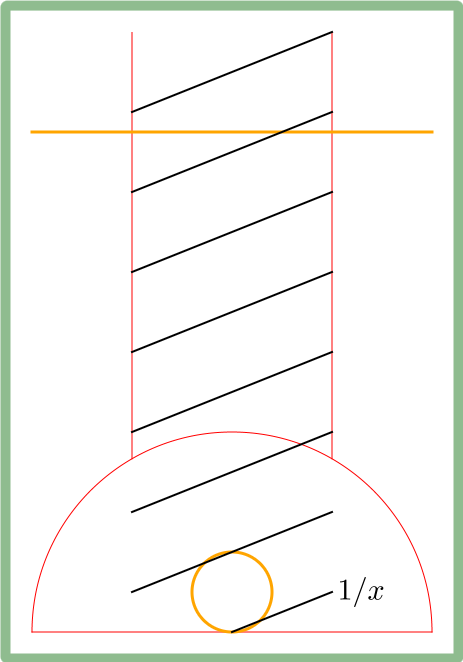
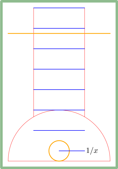
Figure 6.1. The black lines are part of the curve $\mathrm{SL}_{2}\left(\mathbb{Z}\right)Au_{x}$ as viewed in the hyperbolic plane modulo $u_{1}$. On the right, the blue lines are “approximations” of the black lines which are horocycles. The orange circle through the origin is the image of the orange line after applying the Möbius action $z\mapsto-\frac{1}{z}$, so that the area above the line and inside the circle is a neighborhood of the cusp.

Next, we try to approximate each black line in the image above with the corresponding blue horocycle line. In order to do that we write

$$\mathrm{SL}_{2}\left(\mathbb{Z}\right)a\left(T+t\right)u_{x}=\mathrm{SL}_{2}\left(\mathbb{Z}\right)u_{xe^{-T}e^{-t}}a\left(T\right)a\left(t\right)$$

for the integration at times $\left[T,T+\delta\right]$.

There are three parts to this expression:

1. $\mathrm{SL}_{2}\left(\mathbb{Z}\right)u_{xe^{-T}e^{-t}}$ : This part is on the standard horocycle $\mathrm{SL}_{2}\left(\mathbb{Z}\right)U$. However the integral over $t$ is not the Haar measure there, since $t\mapsto xe^{-T}e^{-t}$ is not linear.

2. Multiplication by $a\left(T\right)$ : This will take the horocycle from above and expand it (push it down).

3. Multiplication by $a\left(t\right)$ : When $t$ is very small, this will be negligible.

Part (3) is the simplest one. If $f$ is any compactly supported continues function and $\varepsilon>0$, then by uniform continuity there is some $\delta>0$ such that if $\left\|g\right\|<\delta$ for some $g\in\mathrm{SL}_{2}\left(\mathbb{R}\right)$, then $\left\|g\left(f\right)-f\right\|_{\infty}<\varepsilon$. In particular, if we assume that $t\in\left[0,\delta\right]$, then we can remove the multiplication by $a\left(t\right)$ up to some $\varepsilon$ error which will be as small as we want. Thus, let us ignore this $a\left(t\right)$ from now on.

For part (1), in order to get the Haar measure on the standard horocycle, and not an exponential movement, let us set $s=xe^{-T}e^{-t}$. We then get that

$$\int_{0}^{\delta}f\left(\mathrm{SL}_{2}\left(\mathbb{Z}\right)u_{xe^{-T}e^{-t}}a\left(T\right)\right)\mathrm{dt}=\int_{xe^{-T}e^{-\delta}}^{xe^{-T}}f\left(\mathrm{SL}_{2}\left(\mathbb{Z}\right)u_{s}a\left(T\right)\right)\frac{1}{s}\mathrm{ds}.$$

The last integral is almost the Haar measure on the standard horocycle, where the only problem is the $\frac{1}{s}$. Fortunately, it is inside $\left[e^{-\delta}\frac{x}{e^{T}},\frac{x}{e^{T}}\right]$ and $e^{-\delta}$ is very close to 1, so $\frac{1}{s}$ is almost the constant $\frac{e^{T}}{x}$.

Once we changed $\frac{1}{s}$ to a constant, we integrate over the whole horocycle $\left\lfloor xe^{-T}\left(1-e^{-\delta}\right)\right\rfloor$ times plus an extra $xe^{-T}\left(1-e^{-\delta}\right)-\left\lfloor xe^{-T}\left(1-e^{-\delta}\right)\right\rfloor$. Since $\delta$ is now fixed, if $\frac{x}{e^{T}}$ is large, then this extra integration will be very small. Hence, for example we can assume that $T\leq\ln\left(x\right)\left(1-\varepsilon\right)$.

Putting everything together, we get that up to some small error we have that

$$\frac{1}{\delta}\int_{0}^{\delta}f\left(\mathrm{SL}_{2}\left(\mathbb{Z}\right)a\left(T+t\right)u_{x}\right)\mathrm{dt}\sim\frac{1}{\delta}\frac{e^{T}}{x}\left\lfloor xe^{-T}\left(1-e^{-\delta}\right)\right\rfloor\int_{0}^{1}f\left(\mathrm{SL}_{2}\left(\mathbb{Z}\right)u_{s}a\left(T\right)\right)\mathrm{ds}\sim\int_{0}^{1}f\left(\mathrm{SL}_{2}\left(\mathbb{Z}\right)u_{s}a\left(T\right)\right)\mathrm{ds}.$$

If we also assume that $T$ is not too small, say $T\geq\varepsilon\ln\left(x\right)$, then by the equidistribution of expanding horocycles, the last term is more or less $\mu_{Haar}\left(f\right)$.

Decomposing the segment $\left[0,\ln\left(x\right)\right]$ to $\delta=\delta\left(T,x,\varepsilon\right)$ intervals, we get that up to an error as small as we want (depending on $\varepsilon$ and $\left\|f\right\|_{\infty}$) we have that

$$\frac{1}{\ln\left(x\right)}\int_{0}^{\ln\left(x\right)}f\left(\mathrm{SL}_{2}\left(\mathbb{Z}\right)a\left(t\right)u_{x}\right)\mathrm{dx}\sim\mu_{Haar}\left(f\right).$$

This takes care of a big part of our translated orbit. For times $t<0$, the translated orbit goes to the cusp, so most of it doesn’t contribute to the integral (above the orange line in 6.1), and the time before it leaves the support of $f$ is uniformly bounded, so all together it contributes a constant (which depends only on $\left\|f\right\|$ and $supp\left(f\right)$) e see 56 for the exact details. This constant is of course negligible with respect to our normalization by $\frac{1}{\ln\left(x\right)}$ as $x\to\infty$.

As in our study of continued fractions of rational numbers, our argument fail when $T\geq\ln\left(x\right)$ is too large, but here too there is a symmetry which comes to help us. However, for this argument we need to perturb a bit our measure as follows. Instead of translating by the unipotent matrix $u_{x}$, we will do it using

$$h\left(y\right)=\left(\begin{array}[]{cc}\cosh\left(y/2\right)&\sinh\left(y/2\right)\\ \sinh\left(y/2\right)&\cosh\left(y/2\right)\end{array}\right).$$

The first important observation is that

$$h\left(y\right) =\left(\begin{array}[]{cc}\cosh^{-1/2}\left(y\right)&0\\ 0&\cosh^{1/2}\left(y\right)\end{array}\right)\left(\begin{array}[]{cc}1&\sinh\left(y\right)\\ 0&1\end{array}\right)\left[\overbrace{\left(\cosh\left(y\right)\right)^{-1/2}\left(\begin{array}[]{cc}\cosh\left(y/2\right)&-\sinh\left(y/2\right)\\ \sinh\left(y/2\right)&\cosh\left(y/2\right)\end{array}\right)}^{k\left(y\right)}\right]$$

$$\Rightarrow h\left(y\right) \in a\left(\ln\left(\cosh\left(y\right)\right)\right)\cdot u_{\sinh\left(y\right)}\cdot k\left(y\right),\qquad k\left(y\right)\in\mathrm{SO}_{2}\left(\mathbb{R}\right).$$

This means that

$$\mathrm{SL}_{2}\left(\mathbb{Z}\right)Ah\left(y\right)=\mathrm{SL}_{2}\left(\mathbb{Z}\right)Au_{\sinh\left(y\right)}k\left(y\right).$$

Since $k\left(y\right)$ is in a compact set, the limit as $y\to\infty$ equidistribute if and only if $\mathrm{SL}_{2}\left(\mathbb{Z}\right)Au_{\sinh\left(y\right)}$ equidistribute, and this is exactly the shearing that we discussed before. Also, since
$\left|\sinh\left(y\right)-\cosh\left(y\right)\right|=e^{-y}\to 0$ as $y\to\infty$, for $x=\sinh\left(y\right)$ very big we get that

$$a\left(\ln\left(\cosh\left(y\right)\right)\right)\cdot u_{\sinh\left(y\right)}\sim a\left(\ln\left(x\right)\right)u_{x},$$

so this translation already has inside it our center of symmetry, which is at time $\ln\left(x\right)$ (this is the analogue to translation by ${\scriptstyle\left(\begin{array}[]{cc}m&0\\ 0&1\end{array}\right)}u_{-1/m}$ instead of $u_{-1/m}$ that we saw in the $m$-adic translation).

Recall that in our discussion of the continued fraction of rational numbers we denoted by $\tau$ the reflection $\tau={\scriptstyle\left(\begin{array}[]{cc}0&1\\ 1&0\end{array}\right)}$. It is now easy to see that $\tau h\left(y\right)=h\left(y\right)\tau$ and $a\left(t\right)\tau=\tau a\left(-t\right)$. We then get that

$$\mathrm{GL}_{2}\left(\mathbb{Z}\right)a\left(t\right)h\left(y\right)\tau=\mathrm{GL}_{2}\left(\mathbb{Z}\right)\tau a\left(-t\right)h\left(y\right)=\mathrm{GL}_{2}\left(\mathbb{Z}\right)a\left(-t\right)h\left(y\right),$$

so that flowing forward and backward in time is the same up to this reflection. In particular, in order to show equidistribution when $y\to\infty$, it is enough to prove it for $t\in[0,\infty)$.

Going back to the unipotent translation by $u_{x}$, we get that the times $[\ln\left(x\right),\infty)$ are the mirror image of $(-\infty,\ln\left(x\right)]$, so it is enough to show equidistribution for $t\leq\ln\left(x\right)$ which we already have shown.

Now that we have both the equidistribution for the $m$-adic translations, and the real translations, we can combine both of these ideas to get equidistribution for combined translations. This will be done in 10, and other than it being more technical, it contains no new ideas.

Remark 11.

It is interesting to understand the symmetry mentioned above in the hyperbolic plane. The curve $h\left(x\right)\left(i\right),\;x\in\mathbb{R}$ is simply the upper half of the unit circle $y=\sqrt{1-x^{2}}$. This means that the mid point in this visualization is on that half circle. Our two cutoffs right after our measure “comes” from the cusp and before it “returns” to the cusp are when it intersect the standard horocycle and its reflection via $z\mapsto-\frac{1}{z}$.

7. Shearing over the adeles

Up until now we saw two types of equidistribution phenomena. The first started with measures coming from continued fractions of rational numbers, which we reinterpreted as measures on the space of unimodular lattices $\mathrm{SL}_{2}\left(\mathbb{Z}\right)\backslash\mathrm{SL}_{2}\left(\mathbb{R}\right)$, where each one was a finite average over $A$-orbits. We then saw a more natural point of view for each such measure, namely as a projection of a translation of a single diagonal orbit in $\mathrm{GL}_{2}\left(\mathbb{Z}\left[\frac{1}{m}\right]\right)\backslash\mathrm{GL}_{2}\left(\mathbb{R}\right)\times\mathrm{GL}_{2}\left(\mathbb{Q}_{m}\right)$ where the translation is done in the $\mathbb{Q}_{m}$-coordinate by the matrix $u_{-1/m}$.

The phenomena of translating a diagonal orbit with a unipotent matrix is called shearing. To get some intuition, we saw how the shearing process in $\mathrm{SL}_{2}\left(\mathbb{Z}\right)\backslash\mathrm{SL}_{2}\left(\mathbb{R}\right)$ leads to expanding horocycles, which we can use to prove equidistribution. Actually, the measures in this case can also be seen as projections of a translated diagonal orbit from $\mathrm{PGL}_{2}\left(\mathbb{Z}\left[\frac{1}{m}\right]\right)\backslash\mathrm{PGL}_{2}\left(\mathbb{R}\right)\times\mathrm{PGL}_{2}\left(\mathbb{Q}_{m}\right)$, where the translation is done in the $\mathbb{R}$-coordinate by the matrix $u_{x}$.

The same shearing argument almost works for our original equidistribution result. The problem is that as $m_{i}\to\infty$, the set $\mathbb{Q}_{m_{i}}$ can change. However, if all the $m_{i}$ are divisible only by primes from a finite set $\left\{p_{1},...,p_{k}\right\}$, then $\mathbb{Q}_{m_{i}}\leq\mathbb{Q}_{\prod p_{i}}=\prod\mathbb{Q}_{p_{i}}$ in which case a similar shearing argument will work. However, if this is not the case, we need to take the product over all the primes, which lead to the definition of the adeles.

The main result of this notes is to combine the two equidistribution results that we saw so far, and to show that they still hold when we need infinitely many primes. As we have already seen, the steps in both of these results are quite similar e finding the important part of the measure, where the rest is “near” the cusp, use a symmetry argument to cut the important part to two so we can then approximate the measure with expanding horocycles, and finally use the result about expanding horocycles. However, there are some differences, mainly where we approximate the horocycles using the shearing effect in the $\mathbb{R}$-coordinate, or approximating using averages on discrete points so that the shearing is in the $\mathbb{Q}_{m}$-coordinate.

In order to continue our investigation, we first need a better understanding of the adele ring, and we begin first with some topological properties of the $p$-adic numbers for primes $p$.

Definition 12.

Let $z=\sum_{N}^{\infty}a_{j}m^{j}\in\mathbb{Q}_{m}$ with $a_{N}\neq 0$. Define the $m$-adic valuation and norm to be

$$val_{m}\left(z\right) =N$$

$$\left|z\right|_{m} =m^{-N}=m^{-val_{m}\left(z\right)}.$$

For $0$ we define $val_{m}\left(0\right)=\infty$ and $\left|0\right|_{m}=0$.

Claim 13.

Let $p$ be a prime number. Then the following holds.

1. The function $\left|\cdot\right|_{p}$ satisfies:

   1. For all $q\in\mathbb{Q}_{p}$ we have $\left|q\right|_{p}\geq 0$ with equality if and only if $q=0$.

   2. (strong triangle inequality) For every $z,w\in\mathbb{Q}_{p}$ we have that $\left|z+w\right|_{p}\leq\max\left(\left|z\right|_{p},\left|w\right|_{p}\right)$ with equality if $\left|z\right|_{p}\neq\left|w\right|_{p}$.

   3. (multiplicative) For every $z,w\in\mathbb{Q}_{p}$ we have that $\left|zw\right|_{p}=\left|z\right|_{p}\left|w\right|_{p}$.

2. $\mathbb{Z}_{p}$ is a compact ring inside $\mathbb{Q}_{p}$.

3. $\mathbb{Q}_{p}$ is a complete field with respect to the $p$-adic norm.

Proof.

1. This is elementary and is left to the reader.

2. Note that if $z=\sum_{N}^{\infty}a_{n}p^{n},w=\sum_{N}^{\infty}b_{n}p^{n}\in\mathbb{Q}_{p}$, then $\left|z-w\right|_{p}\leq p^{-M}$ is exactly the same as $a_{i}=b_{i}$ for all $i<M$.
   If $z_{i}=\sum_{0}^{\infty}a_{i,j}p^{j}\in\mathbb{Z}_{p}$ is any sequence, then we can use a diagonal argument to find a subsequence where for each $j$ the sequence $a_{i,j}$ stabilizes to some $a_{j}$ (recall that $a_{i,j}\in\left\{0,...,p-1\right\}$). From the remark above, it is now easy to check that $\sum_{0}^{\infty}a_{j}p^{j}\in\mathbb{Z}_{p}$ is the limit of this subsequence. Thus, $\mathbb{Z}_{p}$ is sequentially compact and therefore compact.

3. By definition, the closed (and open) balls in $\mathbb{Q}_{p}$ are exactly $p^{n}\mathbb{Z}_{p}$. If $z_{i}$ is any Cauchy sequence, it must be in one of thee balls, which by part (2) is compact, so the limit of $z_{i}$ exists and must be in the same ball and therefore in $\mathbb{Q}_{p}$. We conclude that $\mathbb{Q}_{p}$ is complete.

For uniformity of notation, we will use $\mathbb{Q}_{\infty}$ to denote $\mathbb{R}$. We set $\mathbb{P}$ to be the set of prime numbers in $\mathbb{N}$ and $\mathbb{P}_{\infty}=\mathbb{P}\cup\left\{\infty\right\}$. ∎

Remark 14.

Note that $\mathbb{Q}_{p}$ is a complete field, just like $\mathbb{R}$, and algebraically speaking $\mathbb{Z}_{p}$ behaves similar to $\mathbb{Z}$ e for example both are generated as a topological ring by $1$ in the corresponding norms. However, while in $\mathbb{R}$ the subring $\mathbb{Z}$ is discrete and has finite covolume, the ring $\mathbb{Z}_{p}$ in $\mathbb{Q}_{p}$ is compact and has infinite covolume. Hence, with this point of view $\mathbb{Z}_{p}$ behaves more like $\left[0,1\right]$ in $\mathbb{R}$. This two opposite points of view e algebraic and topological e are quite common when dealing with $p$-adic numbers, namely that sometimes we think of $\mathbb{Z}_{p}$ as $\mathbb{Z}$ and sometimes as $\left[0,1\right]$.

We can now define the adele ring.

Definition 15.

For a finite set $\infty\in S\subseteq\mathbb{P}_{\infty}$, let

$$\mathbb{Q}_{S} :=\prod_{\nu\in S}\mathbb{Q}_{\nu}$$

$$\mathbb{Q}^{\left(S\right)} :=\prod_{\nu\in S}\mathbb{Q}_{\nu}\times\prod_{p\notin S}\mathbb{Z}_{p},$$

both with the product topology. We define the ring of adeles $\mathbb{A}=\mathbb{Q}_{\mathbb{P}_{\infty}}$ to be the union $\bigcup_{S}\mathbb{Q}^{\left(S\right)}$ where $S$ runs over all the finite subsets of $\mathbb{P}_{\infty}$ containing $\infty$. The topology on $\mathbb{A}$ is the induced topology, namely $U$ is open if $U\cap\mathbb{Q}_{S}$ is open in $\mathbb{Q}_{S}$ for any $S$ (or equivalently, it is generated by the open sets in $\mathbb{Q}^{\left(S\right)}$). This is called the restricted product $\mathbb{A}:=\mathbb{R}\times\prod_{p}^{\prime}\mathbb{Q}_{p}$ with respect to $\mathbb{Z}_{p}$, namely sequence $\left(g^{\left(\infty\right)},g^{\left(2\right)},g^{\left(3\right)},...\right)\in\mathbb{R}\times\prod_{p}\mathbb{Q}_{p}$ where $g^{\left(p\right)}\in\mathbb{Z}_{p}$ for almost every $p$.

For each $S\subseteq\mathbb{P}_{\infty}$ set

$$\mathbb{Z}\left[S^{-1}\right]:=\mathbb{Z}\left[\frac{1}{p}\;\mid\;p\in S\backslash\left\{\infty\right\}\right]\leq\mathbb{Q},$$

and embed it diagonally in $\mathbb{Q}_{S}$ for $S$ finite and $S=\mathbb{P}_{\infty}$.

Lemma 16.

For $\infty\in S\subseteq\mathbb{P}_{\infty}$ the group $\mathbb{Z}\left[S^{-1}\right]$ is a cocompact lattice in $\mathbb{Q}_{S}$.

Proof.

We leave it as an exercise to show that $\left(-\frac{1}{2},\frac{1}{2}\right)\times\prod_{p\in S\backslash\left\{\infty\right\}}\mathbb{Z}_{p}$ which is an open set in $\mathbb{Q}_{S}$ interests $\mathbb{Z}\left[S^{-1}\right]$ only in $\left\{0\right\}$, implying that it is discrete in $\mathbb{Q}_{S}$. Moreover, using the restricted product structure, and the Chinese remainder theorem we get that

$$\mathbb{Z}\left[S^{-1}\right]+\left[-\frac{1}{2},\frac{1}{2}\right]\times\prod_{p\in S\backslash\left\{\infty\right\}}\mathbb{Z}_{p}=\mathbb{Q}_{S},$$

so that $\mathbb{Z}\left[S^{-1}\right]$ is cocompact. ∎

Note in particular that for $S=\left\{\infty\right\}$, we just get the well known fact that $\mathbb{Z}$ is a lattice in $\mathbb{R}$. As with the $m$-adic numbers, there is a natural projection $\pi_{S}:\mathbb{Q}\backslash\mathbb{A}\to\mathbb{Z}\left[S^{-1}\right]\backslash\mathbb{Q}_{S}$. First identify $\mathbb{Q}\backslash\mathbb{A}$ with the fundamental domain $[0,1)\times\prod_{p}\mathbb{Z}_{p}$ of $\mathbb{Q}$ in $\mathbb{A}$ and then project to the coordinates in $S$.

An important observations about these projections is that the preimage of every point an orbit of $\prod_{p\notin S}\mathbb{Z}_{p}$ which is compact by Tychonoff’s theorem. It follows that the preimage of any compact set is compact, i.e. these projections are proper.

Trying to understand measures over $\mathbb{Q}\backslash\mathbb{A}$, we first need to understand compactly supported continuous functions on $\mathbb{Q}\backslash\mathbb{A}$. Since $\pi_{S}$ is proper for any finite $S\subseteq\mathbb{P}$ we have the induced homomorphism

$$C_{c}\left(\mathbb{Z}\left[S^{-1}\right]\backslash\mathbb{Q}_{S}\right)\to C_{c}\left(\mathbb{Q}\backslash\mathbb{A}\right).$$

The functions in the image of this map are exactly those which are invariant under the action of $\prod_{p\notin S}\mathbb{Z}_{p}$. A simple application of the Stone Weierstrass theorem shows that the union of these sets of functions, as we run over the finite $S$, is dense in $C_{c}\left(\mathbb{Q}\backslash\mathbb{A}\right)$. This implies that if we want to prove an equidistribution $\mu_{i}\overset{w^{*}}{\longrightarrow}\mu_{Haar}$ on $\mathbb{A}$, it is enough to prove that $\mu_{i}\left(f\right)\to\mu_{Haar}\left(f\right)$ for functions in these images. Alternatively, we need to show the pushforward of the measures $\mu_{i}$ to each one of the $\mathbb{Z}\left[S^{-1}\right]\backslash\mathbb{Q}_{S}$ equidistributes.

There is a similar structure when we work with groups over the adeles, and in particular with the group $\mathrm{GL}_{2}^{1}$ which is the main focus of these notes. There is however one main difference where $\mathrm{GL}_{2}\left(\mathbb{Z}\left[S^{-1}\right]\right)$ is a noncompact lattice in $\mathrm{GL}_{2}^{1}\left(\mathbb{Q}_{S}\right)$ (since $\mathrm{SL}_{2}\left(\mathbb{Z}\right)\backslash\mathrm{SL}_{2}\left(\mathbb{R}\right)$ is noncompact).

We already talked in 5 about our translated orbit for the $S$ finite cases. However, note that this is not the same problem, because we first do the translations in $\mathbb{A}$ and then project down to $\mathbb{Q}_{S}$. This is the point where a single orbit can decompose to several diagonal orbits, and in particular, as we saw, a single translated orbit by $u_{1/m}$ is split up to $\varphi\left(m\right)$ orbits over $\mathbb{R}$.

One of the main parts of our proof will be to show that if our measures equidistribute when pushed to only the real place via $\pi_{\left\{\infty\right\}}$, then we can lift this equidistribution to any $S$. We already saw that if we know that this is true for any finite $S$, than it is true for $S=\mathbb{P}_{\infty}$, so we are left with this lifting problem for finite $S$. We will do this in 8 and we leave the details to that section, but let us just mention the main idea which is interesting in itself.

One of the main problem when working over the adeles, is that there are infinitely many prime place that we can translate in. If the translation was in only finitely many places, then we can use an already known shearing result. To work around this problem we look only on the translation in the real place, which we may assume to be either trivial, or $u_{x_{i}}$ with $x_{i}\to\infty$.

Case 1: There is no translation in the real place.

In this case, all of our measures will be invariant under the same diagonal matrices $A$ in the real place. For such measures, we can use an invariant called the entropy of the measure with respect to $A$. This entropy measures in a sense how close is the measure to being $\mathrm{SL}_{2}\left(\mathbb{R}\right)$-invariant. In particular, the entropy is bounded from above, and it achieves the maximum entropy if and only if it is $\mathrm{SL}_{2}\left(\mathbb{R}\right)$-invariant.

The trick now is to use the fact that when projecting down the entropy can only decrease. Hence, if the projected measures equidistribute, their entropy will converge to the maximal entropy, so the entropy of our original measure must converge to the maximal entropy also. It follows that the limit will be $\mathrm{SL}_{2}\left(\mathbb{R}\right)$-invariant as well. This is of course a much smaller group that $\mathrm{GL}_{2}^{1}\left(\mathbb{A}\right)$, however, because we look on the quotient space $\mathrm{GL}_{2}\left(\mathbb{Q}\right)\backslash\mathrm{GL}_{2}^{1}\left(\mathbb{A}\right)$, the group $\mathrm{GL}_{2}\left(\mathbb{Q}\right)$ “mixes” the space together, so invariance under the small group $\mathrm{SL}_{2}\left(\mathbb{R}\right)$ will automatically imply a larger invariance which is almost the whole group.

Case 2: The translations in the real place go to infinity.

In this case we can no longer use the entropy argument, because our measure are not $A$-invariant. However, we already saw that unipotent translations of $A$-orbits become more and more like unipotent orbits. More specifically, if a measure $\mu$ is $A$ invariant, and we consider translations $\mu_{i}=u_{x_{i}}\left(\mu\right)$ as $x_{i}\to\infty$, then $\mu_{i}$ will be invariant under

$$u_{x_{i}}a\left(t\right)u_{-x_{i}}=a\left(t\right)u_{\left(e^{t}-1\right)x_{i}}.$$

Fixing some constant $c$, we can choose $t_{i}$ such that $\left(e^{t_{i}}-1\right)x_{i}=c$ and note that since $x_{i}\to\infty$ we have that $t_{i}\to 0$. It follows that $\mu_{i}$ is $a\left(t_{i}\right)u_{c}$ invariant and $a\left(t_{i}\right)\to a\left(0\right)=Id$, so any limit measure will be invariant under $u_{c}$. As $c$ was arbitrary, the limit measure will be invariant under the unipotent group $U$.

This is very helpful, since we can now use Ratner’s classification theorem of unipotent invariant measures to conclude that our limit measure is algebraic e it is supported on an orbit of some unimodular subgroup $L\leq\mathrm{GL}_{2}^{1}\left(\mathbb{A}\right)$ which contain $U$. At this point we will show that if the projection to $\mathrm{SL}_{2}\left(\mathbb{Z}\right)\backslash\mathrm{SL}_{2}\left(\mathbb{R}\right)$ is the Haar measure, then $L$ must contain all of $\mathrm{SL}_{2}\left(\mathbb{R}\right)$. We can now continue like in case 1 and conclude that our measure must be $\mathrm{GL}_{2}^{1}\left(\mathbb{A}\right)$-invariant.

These are all the main steps for the full equidistribution over the adeles, namely first prove equidistribution only in the projection to the real place, and then use either $A$-invariance and entropy or $U$-invariance and Ratner’s theorem to lift the equidistribution to all of the adeles.

Part II Proofs and Details

Now that we have seen all of the main ideas and steps leading from our problem about continued fractions of rational to shearing over the adeles, we turn to give the details behind these ideas. We begin in 8 where we give the definitions for the space of lattices over the adeles. This space has the standard space of Euclidean lattices as its quotient, and in particular the Haar measure on this space is pushed forward to the Haar measure on the Euclidean lattices. In that subsection we will give some natural conditions which implies that the converse holds as well, namely we can lift the equidistribution in the real place to an equidistribution over all the adeles.

Once we have these notations and the lifting result, we define in 9 the diagonal orbit through the origin, the locally finite, diagonal invariant measure it supports and its translations. Using the Iwasawa decomposition, we will see that for equidistribution results for general translations, it is enough to prove it for unipotent translation, or in other words, we need to prove that the shearing process holds over the adeles. In particular we will show that these orbit translation measures satisfy automatically the extra conditions needed for the lifting result from 8. To simplify the notations, we restrict the discussion in this section to dimension 2, though the most of results hold for a general dimension.

Finally, in 10 we prove that in dimension 2, when pushed to the real place our orbit translation measures equidistribute. This equidistribution result together with the conditions that we prove in 9 allow us to use the lifting result from 8 and to get the full equidistribution result over the adeles. This result can be proved for some specific translations in higher dimension (see for example [1]), however since we don’t know if it holds in general dimension (and even what is the right formulation), we stay only in dimension 2.

8. Adelic Lifting

The main goal of this section is to provide some natural conditions on a measure on the space of adelic lattices, such that it will be the Haar measure there if and only if its pushforward to the space of standard Euclidean lattices is the Haar measure there. We start by fixing our notations for working with the adeles.

8.1. Adelic lattices - notations

It is well known that the space of unimodular lattice in $\mathbb{R}^{d}$ can be identified with $\mathrm{SL}_{d}\left(\mathbb{Z}\right)\backslash\mathrm{SL}_{d}\left(\mathbb{R}\right)$. The main goal of this subsection is to extend this presentation to the adelic setting and to fix the notation for the rest of these notes.

Let $\mathbb{P}$ be all the primes in $\mathbb{N}$, and let $\mathbb{P}_{\infty}=\mathbb{P}\cup\left\{\infty\right\}$ be the set of all places over $\mathbb{Q}$. Unless stated otherwise, the sets $S\subseteq\mathbb{P}_{\infty}$ that we work with will always contain $\infty$. For a subset $S\subseteq\mathbb{P}_{\infty}$ (possibly infinite) we let

$$\mathbb{Q}_{S}=\prod_{p\in S}^{\prime}\mathbb{Q}_{p},\quad\;\mathbb{Z}\left[S^{-1}\right]:=\mathbb{Z}\left[\frac{1}{p}:p\in S\backslash\left\{\infty\right\}\right],$$

where $\prod^{\prime}$ is the restricted product with respect to $\mathbb{Z}_{p}\leq\mathbb{Q}_{p}$. We consider $\mathbb{Z}\left[S^{-1}\right]$ as embedded diagonally in $\mathbb{Q}_{S}$ and it is well known that under this embedding $\mathbb{Z}\left[S^{-1}\right]$ is a lattice in $\mathbb{Q}_{S}$. We shall usually write elements $x\in\mathbb{Q}_{S}$ (and in other such products) as $x=\left(x^{\left(\infty\right)},x^{\left(p_{1}\right)},x^{\left(p_{2}\right)},...\right)$ where $p_{i}\in S$ are the primes. We denote by $x^{\left(f\right)}$ the element $x^{\left(f\right)}=\left(x^{\left(p_{1}\right)},x^{\left(p_{2}\right)},...\right)\in\prod_{p}^{\prime}\mathbb{Q}_{p}$, and using the diagonal embedding, if $x\in\mathbb{Z}\left[S^{-1}\right]$, then we also write $x^{\left(f\right)}=\left(x,x,x,...\right)\in\prod_{p}^{\prime}\mathbb{Q}_{p}$. We will mainly be interested with $S=\mathbb{P}_{\infty}$ and $S$ finite (and in particular $S=\left\{\infty\right\}$).

We similarly extend these notation to $\mathbb{Q}_{S}^{d},\;\mathbb{Z}\left[S^{-1}\right]^{d}$ for any dimension $d\geq 1$ and later on to groups over $\mathbb{Q}_{S}$. Since $\mathbb{Q}_{S}$ is generally not a field (unless $S=\left\{\infty\right\}$), the space $\mathbb{Q}_{S}^{d}$ is not a vector space, but it is a $\mathbb{Q}_{S}$-module, namely we can multiply by elements from $\mathbb{Q}_{S}$. As in vector spaces, modules over commutative rings always have a basis, and many of the results for vector spaces hold here as well.

Note that for $S=\left\{\infty\right\}$, the notation above is just $\mathbb{Q}_{S}=\mathbb{R},\;\mathbb{Z}\left[S^{-1}\right]=\mathbb{Z}$ which is the original example of a lattice. In general we have two definitions for Euclidean lattices in $\mathbb{R}^{d}$ - the first is a discrete, finite covolume subgroup of $\mathbb{R}^{d}$ and the second is the $\mathbb{Z}$-span of a basis of $\mathbb{R}^{d}$. We now extend this notion to general $S$.

Definition 17.

Fix some $d\geq 1$, $S\subseteq\mathbb{P}_{\infty}$ and let $L\leq\mathbb{Q}_{S}^{d}$.

1. A $\mathbb{Z}\left[S^{-1}\right]$-module in $\mathbb{Q}_{S}^{d}$ is a subgroup $L\leq\mathbb{Q}_{S}^{d}$ closed under multiplication by $\mathbb{Z}\left[S^{-1}\right]$.

2. A lattice in $\mathbb{Q}_{S}^{d}$ is a $\mathbb{Z}\left[S^{-1}\right]$-module which is discrete and cocompact.

3. We say that a lattice is unimodular, if it has covolume 1 (with the standard Haar measure on $\mathbb{Q}_{S}^{d}$).

As in the real case, one can show that $L\leq\mathbb{Q}_{S}^{d}$ is a lattice, if and only if it is spanned over $\mathbb{Z}\left[S^{-1}\right]$ by a $\mathbb{Q}_{S}$ basis of $\mathbb{Q}_{S}^{d}$.

Example 18.

$\mathbb{Z}\left[S^{-1}\right]$ is a unimodular lattice in $\mathbb{Q}_{S}$. For discreteness, since $\mathbb{Z}\left[S^{-1}\right]$ is a group it is enough to show that $0$ is separated from all the other point, and indeed it is the unique point in $\left(-1,1\right)\times{\displaystyle\prod_{p\in S\backslash\left\{\infty\right\}}}\mathbb{Z}_{p}$. In addition the compact set $\left[0,1\right]\times{\displaystyle\prod_{p\in S\backslash\left\{\infty\right\}}}\mathbb{Z}_{p}$ is a fundamental domain, so that $\mathbb{Z}\left[S^{-1}\right]$ is a lattice. Similarly $\mathbb{Z}\left[S^{-1}\right]^{d}$ is a unimodular lattice in $\mathbb{Q}_{S}^{d}$.

Next, we set $\mathrm{GL}_{d}\left(\mathbb{Q}_{S}\right):=\prod_{\nu\in S}^{\prime}\mathrm{GL}_{d}\left(\mathbb{Q}_{\nu}\right)$ where the restricted product is with respect to $\mathrm{GL}_{d}\left(\mathbb{Z}_{p}\right)$. The group $\mathrm{GL}_{d}\left(\mathbb{Q}_{S}\right)$ acts transitively on the space of $d$-dimensional lattices in $\mathbb{Q}_{S}^{d}$, and the stabilizer of $\mathbb{Z}\left[S^{-1}\right]^{d}$ is $\mathrm{GL}_{d}\left(\mathbb{Z}\left[S^{-1}\right]\right)$ (embedded diagonally). Thus, just like in the real case, we can identify this space of lattices in $\mathbb{Q}_{S}^{d}$ with $\mathrm{GL}_{d}\left(\mathbb{Z}\left[S^{-1}\right]\right)\backslash\mathrm{GL}_{d}\left(\mathbb{Q}_{S}\right)$.

If we want to restrict our attention to unimodular lattice, we need to know how an element in $\mathrm{GL}_{d}\left(\mathbb{Q}_{S}\right)$ changes the measure in $\mathbb{Q}_{S}^{d}$. As in the real case, this change can be measured by the determinant of the matrix.

Definition 19.

Fix some $d\geq 1$ and $\infty\in S\subseteq\mathbb{P}_{\infty}$.

1. For $x=\left(x^{\left(\nu\right)}\right)_{\nu\in S}\in\mathbb{Q}_{S}$, we define $\left|x\right|=\left|x\right|_{S}:=\prod_{\nu\in S}\left|x^{\left(\nu\right)}\right|_{\nu}\in\mathbb{R}_{\geq 0}$, where $\left|\cdot\right|_{\nu}$ is the standard norm on $\mathbb{Q}_{\nu}$.

2. We define $\det=\det_{S}:\mathrm{GL}_{d}\left(\mathbb{Q}_{S}\right)\to\mathbb{Q}_{S}$ by applying determinant in each place. We further write $\left|\det\right|$ to be the composition $\left|\det\right|:\mathrm{GL}_{d}\left(\mathbb{Q}_{S}\right)\overset{\det}{\to}\mathbb{Q}_{S}\overset{\left|\cdot\right|_{S}}{\to}\mathbb{R}$.
   

Note that by the definition of restricted product, if $x=\left(x^{\left(\nu\right)}\right)_{\nu\in S}\in\mathbb{Q}_{S}$, then $x^{\left(p\right)}\in\mathbb{Z}_{p}$ for almost every prime $p\in S$ and therefore $\left|x^{\left(p\right)}\right|_{p}\leq 1$. It follows that $\left|x\right|=\prod_{\nu\in S}\left|x^{\left(\nu\right)}\right|_{\nu}$ is well defined, though it can be zero even if $x$ doesn’t have any zero entries. However, if all the entries are nonzero and $x^{\left(p\right)}\in\mathbb{Z}_{p}^{\times}$ for almost every $p$, or equivalently $\left|x^{\left(p\right)}\right|_{p}=1$, then we get that $\left|x\right|>0$. In particular we see that for $g\in\mathrm{GL}_{d}\left(\mathbb{Q}_{S}\right)$ we have that $\left|\det\right|\left(g\right)>0$. Furthermore, for $x\in\mathbb{Z}\left[S^{-1}\right]^{\times}$, by the product formula we have that $\left|x\right|_{S}=1$, implying that $\left|\det\right|\left(g\right)=1$ for $g\in\mathrm{GL}_{d}\left(\mathbb{Z}\left[S^{-1}\right]\right)$.

It can now be shown that for $\Omega\subseteq\mathbb{Q}_{S}^{d}$ and $g\in\mathrm{GL}_{d}\left(\mathbb{Q}_{S}\right)$, the measure of $g\left(\Omega\right)$ is the measure of $\Omega$ times $\left|\det\right|\left(g\right)$. With this in mind we define

$$G_{S} =\mathrm{GL}_{d}^{1}\left(\mathbb{Q}_{S}\right):=\left\{g\in\mathrm{GL}_{n}\left(\mathbb{Q}_{S}\right)\;\mid\;\left|\det\right|\left(g\right)=1\right\},$$

$$\Gamma_{S} =\mathrm{GL}_{d}\left(\mathbb{Z}\left[S^{-1}\right]\right),$$

$$X_{S} =\Gamma_{S}\backslash G_{S},$$

so that $X_{S}$ can be identified with the space of unimodular lattices in $\mathbb{Q}_{S}^{d}$. For $S=\left\{\infty\right\}$ and $S=\mathbb{P}_{\infty}$, we will also use $G_{\mathbb{R}}:=G_{\left\{\infty\right\}}$, $G_{\mathbb{A}}=G_{\mathbb{P}_{\infty}}$ and similarly for $\Gamma_{S}$ and $X_{S}$.

The space $X_{S}$ is locally compact, second countable Hausdorff spaces and has the natural $G_{S}$-action from the right. Moreover, the group $G_{S}$ is unimodular and $\Gamma_{S}\leq G_{S}$ is a lattice, so $X_{S}$ supports a $G_{S}$-invariant probability measure which we denote by $\mu_{Haar,S}$.

Finally, as a sanity check, if $S=\left\{\infty\right\}$, then $X_{S}$ is simply $\mathrm{GL}_{d}\left(\mathbb{Z}\right)\backslash\mathrm{GL}_{d}^{1}\left(\mathbb{R}\right)$. Both of the groups $\mathrm{GL}_{d}\left(\mathbb{Z}\right),\mathrm{GL}_{d}^{1}\left(\mathbb{R}\right)$ have the index two subgroup $\mathrm{SL}_{d}\left(\mathbb{Z}\right)$ and $\mathrm{SL}_{d}\left(\mathbb{R}\right)$ respectively, so that $X_{S}\cong\mathrm{SL}_{d}\left(\mathbb{Z}\right)\backslash\mathrm{SL}_{d}\left(\mathbb{R}\right)$ is the standard space of $d$-dimensional unimodular lattices in $\mathbb{R}^{d}$.

Remark 20.

The groups $\mathrm{GL}_{d}^{1}$ and $\mathrm{PGL}_{d}$ are not that far off from each other, and one can actually prove all of the results here for $\mathrm{PGL}_{d}$ instead. However, we choose to work with $\mathrm{GL}_{d}^{1}$ since it simplifies many of the notation, and in particular we work with matrices and not equivalence classes modulo the center. This allows us, for example, to have the generalization of Mahler criterion that we prove in A.

The next step is to connect between the spaces $X_{S}$ for different $S\subseteq\mathbb{P}_{\infty}$. For any $\tilde{S}\subseteq S$ the standard projection $\mathrm{GL}_{d}\left(\mathbb{Q}_{S}\right)\to\mathrm{GL}_{d}\left(\mathbb{Q}_{\tilde{S}}\right)$ doesn’t induce a well defined projection for the quotient spaces $X_{S}\to X_{\tilde{S}}$. However, there is such a natural projection $\pi_{\tilde{S}}^{S}:X_{S}\to X_{\tilde{S}}$ which is defined as follows. Consider first the natural open embedding:

$$H_{S}:=\mathrm{SL}_{d}\left(\mathbb{R}\right)\times\prod_{p\in S}\mathrm{GL}_{d}\left(\mathbb{Z}_{p}\right)\hookrightarrow G_{S}.$$

Note that while the elements $g\in G_{S}$ are such that the product of $\left|\det\left(g^{\left(\nu\right)}\right)\right|_{\nu}$ is 1, the elements $h\in H_{S}$ satisfy $\left|\det\left(h^{\left(\nu\right)}\right)\right|_{\nu}=1$ for all $\nu$.

Claim 21.

The map $H_{S}\hookrightarrow G_{S}$ induces a homeomorphism $\mathrm{SL}_{d}\left(\mathbb{Z}\right)\backslash H_{S}\cong\Gamma_{S}\backslash G_{S}$.

Proof.

We claim that the $H_{S}$ acts transitively on $X_{S}$ and since $H_{S}\cap\Gamma_{S}=\mathrm{SL}_{d}\left(\mathbb{Z}\right)$, the claim will follow. Let $g\in G_{S}$, and let $q\in\Gamma_{S}$ be the identity matrix with

$$sign\left(g^{\left(\infty\right)}\right)\prod_{p\in S\backslash\left\{\infty\right\}}\left|\det\left(g^{\left(p\right)}\right)\right|_{p}$$

in the $\left(1,1\right)$-coordinate. It then follows that for every prime $p\in S\backslash\left\{\infty\right\}$ we have that

$$\left|\det\left(qg^{\left(p\right)}\right)\right|_{p}=\left|\det\left(q\right)\right|_{p}\left|\det\left(g^{\left(p\right)}\right)\right|_{p}=\left|\det\left(g^{\left(p\right)}\right)\right|_{p}^{-1}\left|\det\left(g^{\left(p\right)}\right)\right|_{p}=1.$$

Moreover, since $\left|\det_{S}\left(qg\right)\right|=1$ and $\det\left(qg^{\left(\infty\right)}\right)>0$, we also get that $\det\left(qg^{\left(\infty\right)}\right)=1$. In other words we have shown that $qg\in H_{S}$ which proves the transitivity. ∎

In this new presentation the lattice $\mathrm{SL}_{d}\left(\mathbb{Z}\right)$ is fixed, so that given $\infty\in\tilde{S}\subseteq S\subseteq\mathbb{P}_{\infty}$, the standard projection $H_{S}\to H_{\tilde{S}}$ induces the projection

$$\pi_{\tilde{S}}^{S}:X_{S}\cong\mathrm{SL}_{d}\left(\mathbb{Z}\right)\backslash H_{S}\to\mathrm{SL}_{d}\left(\mathbb{Z}\right)\backslash H_{\tilde{S}}\cong X_{\tilde{S}}.$$

The preimage of every point is then an orbit of $\prod_{p\in S\backslash\tilde{S}}\mathrm{GL}_{d}\left(\mathbb{Z}_{p}\right)$ which is compact, implying that $\pi_{\tilde{S}}^{S}$ is proper.

In general, the presentation with $H_{S}$ is much more convenient to work with, because it let us connect between the different $X_{S}$. On the other hand, we want to act with the larger group $G_{S}$, so throughout these notes we will need to move back and forth between these two presentations.

Just like the space of Euclidean lattices, we have a generalized Mahler criterion for the space of $S$-adic lattices. We will prove this criterion in A.

Definition 22.

For $h\in H_{S}$ define

$$ht_{S}\left(\mathbb{Z}\left[S^{-1}\right]^{d}h\right)=ht_{\infty}\left(\mathbb{Z}^{d}h^{\left(\infty\right)}\right):=\left(\min_{0\neq v\in\mathbb{Z}^{d}}\left\|vh^{\left(\infty\right)}\right\|\right)^{-1}.$$

Lemma 23 (Generalized Mahler’s criterion).

A set $\Omega\subseteq X_{S}$ is bounded if and only if $ht_{S}\left(\Omega\right)$ is bounded.

We can identify $G_{\tilde{S}}$ as a subgroup of $G_{S}$ as the elements which are the identity in all of the entries in $S\backslash\tilde{S}$. It is now not hard to check that $\pi_{\tilde{S}}^{S}$ is $G_{\tilde{S}}$-equivariant. In particular a $G_{S}$-invariant probability measure on $X_{S}$ will be pushed down to a $G_{\tilde{S}}$.

For the converse direction, suppose now that $\mu_{S}$ is a probability measure on $X_{S}$ such that it pushforward $\pi_{\mathbb{R}}^{S}\left(\mu_{S}\right)$ to the “smallest” possible space $X_{\mathbb{R}}$ is the $\mathrm{SL}_{d}\left(\mathbb{R}\right)$-invariant measure. Trying to lift this invariance back to $\mu_{S}$ we encounter two problems:

1. Show that $\mu_{S}$ itself is $\mathrm{SL}_{d}\left(\mathbb{R}\right)$-invariant.

2. Show that $\mu_{S}$ is invariant under $G_{S\backslash\left\{\infty\right\}}$ as well.

These two conditions will require us to show some invariance condition of $\mu_{S}$. In order to get (1) we will need an extra invariance condition that $\mu_{S}$ is invariant under the diagonal or unipotent flow in $\mathrm{SL}_{d}\left(\mathbb{R}\right)$ (which is done in 8.2). Once we have this $\mathrm{SL}_{d}\left(\mathbb{R}\right)$-invariance, we automatically get in 8.3 invariance under a larger group - this is because $\mu_{S}$ is a measure on $\Gamma_{S}\backslash G_{S}$ and $\Gamma_{S}$ “mixes” the real coordinate with the coordinates in $S\backslash\left\{\infty\right\}$. However, this will not provide a full $G_{S}$-invariance, but if $\left|S\right|<\infty$, and we have some extra uniformity condition over the primes in $S\backslash\left\{\infty\right\}$ , then we will get this invariance. Finally, For $\left|S\right|$ infinite, by the structure of restricted products, it will suffice to prove $G_{S_{0}}$-invariance for every $\infty\in S_{0}\subseteq S$ with $\left|S_{0}\right|$ finite. This final part will be done in 8.3.1, where we will also prove the main lifting result in 37.

8.2. Lifting the $\mathrm{SL}_{d}\left(\mathbb{R}\right)$-invariance

Let us fix $S\subseteq\mathbb{P}_{\infty}$ finite and let $\mu_{S}$ be a probability measure on $X_{S}$ such that $\pi_{\mathbb{R}}^{S}\left(\mu_{S}\right)=\mu_{Haar,\mathbb{R}}$. We begin with the proof of lifting the $\mathrm{SL}_{d}\left(\mathbb{R}\right)$-invariance of $\pi_{\mathbb{R}}^{S}\left(\mu_{S}\right)$ to the $\mathrm{SL}_{d}\left(\mathbb{R}\right)$-invariance of $\mu_{S}$ itself. The idea is to use either diagonal or unipotent invariance, and the main tools to study these are maximal entropy for the diagonal case and Ratner’s classification theorem for the unipotent case. However, both of these theorems are usually formulated for spaces of the form $\mathbb{G}\left(\mathbb{Z}\left[S^{-1}\right]\right)\backslash\mathbb{G}\left(\mathbb{Q}_{S}\right)$ for some finite $S\subseteq\mathbb{P}_{\infty}$, and our space $X_{S}=\mathrm{GL}_{d}\left(\mathbb{Z}\left[S^{-1}\right]\right)\backslash\mathrm{GL}_{d}^{1}\left(\mathbb{Q}_{S}\right)$ is not exactly like this. So instead, we will first prove the claim for measures over

$$Y_{S}=\mathrm{SL}_{d}\left(\mathbb{Z}\left[S^{-1}\right]\right)\backslash\mathrm{SL}_{d}\left(\mathbb{Q}_{S}\right),$$

which can be viewed as subspaces of $X_{S}$ via the embedding $\mathrm{SL}_{d}\left(\mathbb{Q}_{S}\right)\hookrightarrow\mathrm{GL}_{d}^{1}\left(\mathbb{Q}_{S}\right)$, and in the end we will show how to extend it to $X_{S}$.

Let us first recall the required results, starting with maximal entropy.

We give here the basic definitions for entropy, though we will not really use them, and only use the result about the maximal entropy. For more details about entropy in homogeneous spaces, see [3, 5].

Definition 24.

Let $\left(X,\mu,T\right)$ be a measure-preserving system. For a finite measurable partition $\mathcal{P}$ of $X$ and $n\in\mathbb{N}$ we write $\mathcal{P}_{n}=\bigvee_{0}^{n-1}T^{-i}\mathcal{P}$ where $\vee$ is the joint refinement operation.

1. For a finite measurable partition $\mathcal{P}$ of $X$ we write $H_{\mu}\left(\mathcal{P}\right)=-{\displaystyle\sum_{P\in\mathcal{P}}}\mu\left(P\right)\ln\left(P\right)$ where
   $0\ln\left(0\right)=0$ and set $H_{\mu}\left(T,\mathcal{P}\right)={\displaystyle\lim_{n\to\infty}}\frac{1}{n}H_{\mu}\left(\mathcal{P}^{n}\right)$ (and this limit always exists).

2. The entropy of $\mu$ with respect to $T$ is defined to be $h_{\mu}\left(T\right)=\sup_{\mathcal{P}}H_{\mu}\left(\mathcal{P},T\right)$ where the supremum is over finite measurable partitions of $X$.

On each of the lattice spaces $X_{S}$ we have the action of $\mathrm{SL}_{d}\left(\mathbb{R}\right)$ and in particular of its positive diagonal subgroup $A$. Recall that we can identify this subgroup with $\mathbb{R}_{0}^{d}:=\left\{\left(t_{1},...,t_{d}\right)\;\mid\;\sum t_{i}=0\right\}$ via $\bar{t}\mapsto a\left(\bar{t}\right):=diag\left(e^{t_{1}},...,e^{t_{d}}\right)$. When the action $T$ is a multiplication by some certain elements from $A$, the maximal possible entropy can be achieved only with the $\mathrm{SL}_{d}\left(\mathbb{R}\right)$-invariant measures. Let us make this statement more precise.

Definition 25.

For the spaces $X_{S},S\subseteq\mathbb{P}$ finite and $\bar{t}\in\mathbb{R}_{0}^{d}$, we shall denote by $T_{\bar{t}}:X_{S}\to X_{S}$ the right multiplication $T_{a}\left(x\right)=xa$ where $a=a\left(\bar{t}\right):=\mathrm{diag}\left(e^{t_{1}},...,e^{t_{d}}\right)\in\mathrm{SL}_{d}\left(\mathbb{R}\right)$. The stable horosphere subgroup of $a$ is defined to be

$$U_{a} :=\left\{g\in\mathrm{SL}_{d}\left(\mathbb{R}\right)\;\mid\;a^{n}ga^{-n}\to e\;as\;n\to\infty\right\}$$

$$=\left\{I+\sum_{t_{i}<t_{j}}\alpha_{i,j}e_{i,j}\in\mathrm{SL}_{d}\left(\mathbb{R}\right)\;\mid\;\alpha_{i,j}\in\mathbb{R}\right\}.$$

We will further use the notation $U_{i,j}=\left\{I+ue_{i,j}\in\mathrm{SL}_{d}\left(\mathbb{R}\right)\;\mid\;u\in\mathbb{R}\right\}$ for $i\neq j$ and note that $U_{a}=\left\langle U_{i,j}\;\mid\;t_{i}<t_{j}\right\rangle$.

In particular if $t_{1}\leq t_{2}\leq\cdots\leq t_{d}$, then $U_{a}$ is a subgroup of the unipotent upper triangular matrices, and it equals this group if all of the $t_{i}$ are distinct. The matrix $a$ acts by conjugation on the Lie algebra $\mathfrak{U}_{a}=span_{\mathbb{R}}\left\{e_{i,j}\;\mid\;t_{i}<t_{j}\right\}$ of $U_{a}$, where each $e_{i,j}$ is an eigenvector with eigenvalue $e^{t_{i}-t_{j}}$. An important constant that we will use is $\Psi_{a}:=-\ln\left|\det\left(Ad_{a}\mid_{\mathfrak{U}_{a}}\right)\right|$ which measures how much conjugation by $a$ “stretches” $U_{a}$.

Example 26.

1. For the matrix $a=\left(\begin{array}[]{cc}e^{-t/2}&0\\ 0&e^{t/2}\end{array}\right)$, the stable horospherical subgroup is $U_{a}=\left\{\left(\begin{array}[]{cc}1&u\\ 0&1\end{array}\right)\;\mid\;u\in\mathbb{R}\right\}$ and the Lie algebra is $\mathfrak{U}_{a}=\left\{ue_{1,2}=\left(\begin{array}[]{cc}0&u\\ 0&0\end{array}\right)\;\mid\;u\in\mathbb{R}\right\}$ with a single eigenvalue $\frac{1}{e}$. Hence $\Psi_{a}=-\ln\left|\det\left(Ad_{a}\mid_{\mathfrak{U}_{a}}\right)\right|=-\ln\left(\frac{1}{e}\right)=1$.

2. In higher dimension, for $a=\mathrm{diag}\left(e^{-\frac{(d-1)}{d}},e^{\frac{1}{d}},...,e^{\frac{1}{d}}\right)$ we have $\mathfrak{U}_{a}=\left\{\sum_{2}^{d}u_{i}e_{1,i}\;\mid\;u_{i}\in\mathbb{R}\right\}$ and the eigenvalue $\frac{1}{e}$ has multiplicity $d-1$. Hence $\Psi_{a}=-\ln\left|\det\left(Ad_{a}\mid_{\mathfrak{U}_{a}}\right)\right|=d-1$.

3. If $t_{1}\leq t_{2}\leq\cdots\leq t_{d}$, then $\Psi_{a}=-\ln\left|\det\left(Ad_{a}\mid_{\mathfrak{U}_{a}}\right)\right|=\sum_{i<j}\left(t_{j}-t_{i}\right)$.

4. For any $a\in A$ we have that $\Psi_{a}=\Psi_{a^{-1}}$.
   

We can now formulate the maximal entropy result.

Theorem 27 (see Theorems 7.6 and 7.9 in [3]).

Fix some finite set $S\subseteq\mathbb{P}_{\infty}$ , $a=a\left(\bar{t}\right)\in A$ for some $\bar{t}\in\mathbb{R}_{0}^{d}$ and let $\mu_{S}$ be a $T_{a}$-invariant probability measure on $Y_{S}$. Then $h_{\mu_{S}}\left(T_{a}\right)\leq\Psi_{a}$ with equality if and only if $\mu_{S}$ is $U_{a}$-invariant. Similarly $h_{\mu_{S}}\left(T_{a}^{-1}\right)\leq\Psi_{a}$ with equality if and only if $\mu_{S}$ is $U_{a^{-1}}=U_{a}^{tr}$-invariant.

In case that $T$ is invertible, like with $T_{a}$ above, we have that $h_{\mu}\left(T\right)=h_{\mu}\left(T^{-1}\right)$. Thus, an immediate corollary of the theorem above is that if $\mu_{S}$ is a $T_{a}$-invariant probability measure on $Y_{S}$ which has maximal entropy $\Psi_{a}$ with respect to $T_{a}$, then it is $\left\langle U_{a},U_{a}^{tr}\right\rangle=\mathrm{SL}_{d}\left(\mathbb{R}\right)$ invariant.

The second result we need deals with unipotent-invariant measures, in which case we use Ratner’s theorem.

Theorem 28.

(See [14]) Fix some finite $S\subseteq\mathbb{P}_{\infty}$ finite and let $\mu_{S}$ be an ergodic $U$-invariant probability on $Y_{S}$ for some unipotent subgroup $U$ of $\mathrm{SL}_{d}\left(\mathbb{Q}_{S}\right)$. Then there exists a subgroup $H\leq L\leq\mathrm{SL}_{d}\left(\mathbb{Q}_{S}\right)$, such that $\mu_{S}$ is an $L$-invariant probability measure on a closed $L$-orbit in $Y_{S}$.

For such algebraic measures that we get from Ratner’s theorem, we have the following lifting result.

Lemma 29.

Let $S\subseteq\mathbb{P}_{\infty}$ be a finite set and write $\pi=\pi_{\mathbb{R}}^{S}$. Let $\mu_{S}$ be a probability measure on $Y_{S}$ such that:

1. $\mu_{S}$ is an $L$-invariant probability measure on $xL$ where $x\in Y_{S}$ and $L\leq\mathrm{SL}_{d}\left(\mathbb{Q}_{S}\right)$.

2. $L$ contains at least one element $g\in\mathrm{SL}_{d}\left(\mathbb{R}\right)$ which is not $\pm Id$.

3. $supp\left(\pi\left(\mu_{S}\right)\right)=Y_{\mathbb{R}}$.

Then $\mu_{S}$ is $\mathrm{SL}_{d}\left(\mathbb{R}\right)$-invariant.

Proof.

Define $L^{\infty}$ and $L_{\infty}$ be the intersection and projection of $L$ to the real place, namely

$$L^{\infty} =\left\{g\in\mathrm{SL}_{d}\left(\mathbb{R}\right)\;\mid\;\left(g,Id,...,Id\right)\in L\right\},$$

$$L_{\infty} =\left\{g\in\mathrm{GL}_{d}\left(\mathbb{R}\right)\;\mid\;\exists g^{\left(f\right)}\in\prod_{p\in S\backslash\left\{\infty\right\}}\mathrm{SL}_{d}\left(\mathbb{Q}_{p}\right),\;s.t.\;\left(g,g^{\left(p\right)}\right)\in L\right\}.$$

Since $L$ is closed as the stabilizer of $\mu_{S}$, and $\mathrm{SL}_{d}\left(\mathbb{R}\right)$ is closed in $\mathrm{SL}_{d}\left(\mathbb{Q}_{S}\right)$, we see that $L^{\infty}=L\cap\mathrm{SL}_{d}\left(\mathbb{R}\right)$ is closed and it is also easy to see that it is normal in $L_{\infty}$. We shall soon see that condition (3) above implies that $L_{\infty}\cap\mathrm{SL}_{d}\left(\mathbb{R}\right)$ is dense in $\mathrm{SL}_{d}\left(\mathbb{R}\right)$, so that $L^{\infty}\leq\mathrm{SL}_{d}\left(\mathbb{R}\right)$ is actually normal in $\mathrm{SL}_{d}\left(\mathbb{R}\right)$. Using part (2) and the simplicity of $\mathrm{PSL}_{d}\left(\mathbb{R}\right)$, we conclude that $L^{\infty}$ must be all of $\mathrm{SL}_{d}\left(\mathbb{R}\right)$, which is what we wanted to prove.

Thus, we are left to show that the condition $supp\left(\pi\left(\mu_{S}\right)\right)=Y_{\mathbb{R}}$ implies that $L_{\infty}$ is dense in $\mathrm{SL}_{d}\left(\mathbb{R}\right)$.

First, it is easy to check that the pushforward satisfies $\pi\left(supp\left(\mu_{S}\right)\right)\subseteq supp\left(\pi\left(\mu_{S}\right)\right)$, but the converse is true as well. Indeed, fix some $y\in supp\left(\pi\left(\mu_{S}\right)\right)$ and an open neighborhood $y\in V_{0}$ with compact closure. For any open subset $y\in V\subseteq V_{0}$ we have that $\mu_{S}\left(\pi^{-1}\left(V\right)\right)=\left(\pi\mu_{S}\right)\left(V\right)>0$, so we can find $x_{V}\in supp\left(\mu_{S}\right)\cap\pi^{-1}\left(V\right)\subseteq\pi^{-1}\left(\overline{V}_{0}\right)$. Since the last set is compact (using the fact that the map is proper), we conclude that the net $V\mapsto x_{V}$ has a convergent subnet to some $x_{\infty}\in\pi^{-1}\left(\overline{V}_{0}\right)$. Furthermore, since $V\mapsto\pi\left(x_{V}\right)\in V$ converges to $y$, we obtain that $x_{\infty}\in\pi^{-1}\left(y\right)$. Finally, since $supp\left(\mu_{S}\right)$ is closed it follows that $x_{\infty}\in supp\left(\mu_{S}\right)$ so that $y\in\pi\left(supp\left(\mu_{S}\right)\right)$.

By the assumption that $supp\left(\pi\left(\mu_{S}\right)\right)=Y_{\mathbb{R}}$, and since $supp\left(\mu_{S}\right)=xL$, we get that $\pi\left(xL\right)=Y_{\mathbb{R}}$, so we may choose $x=\mathrm{SL}_{d}\left(\mathbb{Z}\left[S^{-1}\right]\right)\cdot h$ for some $h=\left(Id,h^{\left(f\right)}\right)$ where $h^{\left(f\right)}\in{\displaystyle\prod_{p\in S\backslash\left\{\infty\right\}}}\mathrm{SL}_{d}\left(\mathbb{Z}_{p}\right)$.

Letting $\tilde{\Gamma}_{S}=\mathrm{SL}_{d}\left(\mathbb{Z}\left[S^{-1}\right]\right)$, for any $g=\left(g^{\left(\infty\right)},g^{\left(f\right)}\right)\in L$ we can write

$$xg=\tilde{\Gamma}_{S}\left(g^{\left(\infty\right)},h^{\left(f\right)}g^{\left(f\right)}\right)=\tilde{\Gamma}_{S}\left(\gamma g^{\left(\infty\right)},\gamma h^{\left(f\right)}g^{\left(f\right)}\right),$$

where $\gamma\in\tilde{\Gamma}_{S}$ and $\gamma h^{\left(f\right)}g^{\left(f\right)}\in{\displaystyle\prod_{p\in S\backslash\left\{\infty\right\}}}\mathrm{SL}_{d}\left(\mathbb{Z}_{p}\right)$, implying that $\pi\left(xg\right)=\tilde{\Gamma}_{\mathbb{R}}\gamma g^{\left(\infty\right)}$. We conclude that

$$Y_{\mathbb{R}} =\pi\left(xL\right)\subseteq\tilde{\Gamma}_{\mathbb{R}}\cdot\left(\tilde{\Gamma}_{S}L_{\infty}\right)\subseteq\tilde{\Gamma}_{S}L_{\infty},$$

and therefore $\mathrm{SL}_{d}\left(\mathbb{R}\right)\subseteq\tilde{\Gamma}_{S}L_{\infty}$. Let us show that the fact that $\tilde{\Gamma}_{S}$ is countable implies that $L_{\infty}\cap\mathrm{SL}_{d}\left(\mathbb{R}\right)$ is dense in $\mathrm{SL}_{d}\left(\mathbb{R}\right)$.

Fix some $M\in\mathfrak{sl}_{d}\left(\mathbb{R}\right)$ and let $L_{M}=\left\{t\in\mathbb{R}\;\mid\;\exp\left(tM\right)\in L_{\infty}\right\}$ which is a subgroup of $\mathbb{R}$. If we can show that $L_{M}$ is dense in $\mathbb{R}$, then in particular $\exp\left(M\right)\in\overline{L_{\infty}}$. If we can show this for any $M$, then we will get that $L_{\infty}\cap\mathrm{SL}_{d}\left(\mathbb{R}\right)$ is dense in $\mathrm{SL}_{d}\left(\mathbb{R}\right)$.

Fix some $\varepsilon>0$, and for every $0<t<\varepsilon$ write $\exp\left(tM\right)=\gamma_{t}g_{t}$ where $\gamma_{t}\in\tilde{\Gamma}_{S}$ and $g_{t}\in L_{\infty}$. Since there are uncountable such $t$ and $\tilde{\Gamma}_{S}$ is countable, there are $0<t_{1}<t_{2}<\varepsilon$ such that $\gamma_{t_{1}}=\gamma_{t_{2}}$. It follows that $\exp\left(\left(t_{2}-t_{1}\right)M\right)=g_{t_{1}}^{-1}g_{t_{2}}\in L_{\infty}$, so that $t_{2}-t_{1}\in L_{M}\cap\left(0,\varepsilon\right)$. Since $\varepsilon$ was arbitrary, we conclude that $L_{M}$ must be dense in $\mathbb{R}$ and therefore $\overline{L_{\infty}\cap\mathrm{SL}_{d}\left(\mathbb{R}\right)}=\mathrm{SL}_{d}\left(\mathbb{R}\right)$ which was the last result that we needed to complete the proof.

∎

We can now put everything together to get our $\mathrm{SL}_{d}\left(\mathbb{R}\right)$-invariance lifting on $Y_{S}$.

Lemma 30.

Let $S\subseteq\mathbb{P}_{\infty}$ be a finite set and $\mu_{S}$ a probability measure on $Y_{S}$ such that $\mu_{Haar,\mathbb{R}}=\pi_{\mathbb{R}}^{S}\left(\mu_{S}\right)$. Then if $\mu_{S}$ is invariant under a one parameter unipotent subgroup $\left\{u^{t}\;\mid\;t\in\mathbb{R}\right\}\in\mathrm{SL}_{d}\left(\mathbb{R}\right)$ or a diagonal element $Id\neq a\in\mathrm{SL}_{d}\left(\mathbb{R}\right)$, then it is $\mathrm{SL}_{d}\left(\mathbb{R}\right)$-invariant.

Proof.

We claim that we may assume that $\mu_{S}$ is $a$ (resp. $u$) ergodic. Indeed, if $\mu_{S}=\int\mu_{S,\alpha}\mathrm{d\alpha}$ is the ergodic decomposition to $a$ (resp. $u$) ergodic measures, then $\mu_{Haar,\mathbb{R}}=\pi_{\mathbb{R}}^{S}\left(\mu_{S}\right)=\int\pi_{\mathbb{R}}^{S}\left(\mu_{S,\alpha}\right)\mathrm{d\alpha}$ is also a decomposition. Since $\mu_{Haar,\mathbb{R}}$ is both $u$ and $A$-ergodic, then it is an extreme point in the space of invariant probability measures, and therefore this decomposition is trivial - outside of a zero measure set, we have that $\pi_{\mathbb{R}}^{S}\left(\mu_{S,\alpha}\right)=\mu_{Haar,\mathbb{R}}$. Thus, it is enough to prove the lemma for the $A$ (resp. $u$)-invariant and ergodic measures $\mu_{S,\alpha}$.

Assume first that $\mu_{S}$ is $A$-invariant. As the entropy can only decrease in factors, using 27 we obtain that

$$\Psi_{a}=h_{\mu_{Haar,\mathbb{R}}}\left(T_{a}\right)\leq h_{\mu_{S}}\left(T_{a}\right)\leq\Psi_{a},$$

hence $h_{\mu_{S}}\left(T_{a}\right)=\Psi_{a}$ and similarly $h_{\mu_{S}}\left(T_{a}^{-1}\right)=\Psi_{a}$. Using 27 once again we conclude that $T$ is $\left\langle U_{a},U_{a}^{tr}\right\rangle=\mathrm{SL}_{d}\left(\mathbb{R}\right)$-invariant.

If $\mu_{S}$ is $u$-invariant and ergodic under some unipotent matrix in $\mathrm{SL}_{d}\left(\mathbb{R}\right)$, then we can apply Ratner’s theorem which provides condition (1) in 29. Since $u$ is not central, we get condition (2) of that lemma. Finally, we try to lift the Haar measure $\pi_{\mathbb{R}}^{S}\left(\mu_{S}\right)=\mu_{Haar,\mathbb{R}}$, so that condition (3) is satisfied as well. Hence by this lemma we get that $\mu_{S}$ is $\mathrm{SL}_{d}\left(\mathbb{R}\right)$-invariant. ∎

Finally, we want to move from $Y_{S}$ to $X_{S}$. The difference between these two spaces is that in $Y_{S}$ we require all the elements to be of determinant 1, while in $X_{S}$ the product of the norms of the determinant is $1$. To help us move from one space to the other we use the following definitions.

Definition 31.

For $S\subseteq\mathbb{P}_{\infty}$, we define the determinant

$$\det_{S\backslash\left\{\infty\right\}}:G_{S}\overset{\det}{\longrightarrow}\mathbb{R}^{\times}\times{\displaystyle\prod_{p\in S\backslash\left\{\infty\right\}}}\mathbb{Q}_{p}^{\times}\longrightarrow{\displaystyle\prod_{p\in S\backslash\left\{\infty\right\}}}\mathbb{Q}_{p}^{\times}.$$

We identify the elements from ${\displaystyle\prod_{p\in S\backslash\left\{\infty\right\}}}\mathbb{Q}_{p}^{\times}$ asdiagonal matrices in $\mathrm{GL}_{d}\left(\mathbb{Q}_{S}\right)$ via

$$\bar{\alpha}=\left(\alpha^{\left(p_{1}\right)},...,\alpha^{\left(p_{k}\right)}\right)\mapsto g_{\bar{\alpha}}=\left(Id,diag\left(\alpha^{\left(p_{1}\right)},1,...,1\right),...,diag\left(\alpha^{\left(p_{k}\right)},1,...,1\right)\right).$$

Theorem 32.

30 holds for the space $X_{S}$ as well.

Proof.

Let $K^{1}=\left\{\bar{\alpha}\in{\displaystyle\prod_{p\in S\backslash\left\{\infty\right\}}}\mathbb{Q}_{p}^{\times}\;\mid\;\prod\left|\alpha^{\left(p_{i}\right)}\right|_{p_{i}}=1\right\}$. Viewing $Y_{S}$ as a subspace of $X_{S}$ via embedding $\mathrm{SL}_{d}\left(\mathbb{Q}_{S}\right)\hookrightarrow\mathrm{GL}_{d}^{1}\left(\mathbb{Q}_{S}\right)$ we get decompose $X_{S}$ as

$$X_{S}=\bigsqcup_{\bar{\alpha}\in K^{1}}Y_{S}g_{\bar{\alpha}}.$$

This defines the map $X_{S}\to K^{1}$ which sends elements in $Y_{S}g_{\bar{\alpha}}$ to $\bar{\alpha}$. Given a probability measure on $\mu$ on $X_{S}$, we can use disintegration of measures to obtain

$$\mu=\int_{K^{1}}\mu_{\bar{\alpha}}\circ g_{\bar{\alpha}}\mathrm{d\alpha}$$

where for almost every $\bar{\alpha}$, the measure $\mu_{\bar{\alpha}}$ is supported on $Y_{S}$ and $\mathrm{d\alpha}$ is the pushforward of $\mu$ to $K^{1}$. Since $\mathrm{SL}_{d}\left(\mathbb{R}\right)$ acts $Y_{S}$ and commutes with the elements from $K^{1}$, if $\mu$ is $A$ (resp. $U$)- invariant, then we may assume that the $\mu_{\bar{\alpha}}$ are also $A$ (resp. $U$)-invariant for almost every $\bar{\alpha}$. Like in 30 above, projecting this decomposition to $X_{\mathbb{R}}$, we obtain a convex decomposition of the Haar measure, so that 30 implies that $\mu_{\bar{\alpha}}$ is $\mathrm{SL}_{d}\left(\mathbb{R}\right)$-invariant for almost every $\bar{\alpha}$. Finally, this in turn implies that $\mu$ is $\mathrm{SL}_{d}\left(\mathbb{R}\right)$-invariant which is what we wanted to show.

∎

8.3. From $\mathrm{SL}_{d}\left(\mathbb{R}\right)$-invariance to $\mathrm{SL}_{d}\left(\mathbb{R}\right)\times{\displaystyle\prod_{p\in S\backslash\left\{\infty\right\}}}\mathrm{SL}_{d}\left(\mathbb{Z}_{p}\right)$-invariance

Recall that our measure is on the space $X_{S}\cong\mathrm{SL}_{d}\left(\mathbb{Z}\right)\backslash H_{S}$ where $\mathrm{SL}_{d}\left(\mathbb{Z}\right)$ is embedded diagonally in
$H_{S}=\mathrm{SL}_{d}\left(\mathbb{R}\right)\times{\displaystyle\prod_{p\in S\backslash\left\{\infty\right\}}}\mathrm{GL}_{d}\left(\mathbb{Z}_{p}\right)$. In the previous section we showed how to lift Haar measures on $X_{\mathbb{R}}$ to right $\mathrm{SL}_{d}\left(\mathbb{R}\right)$-invariance on $X_{S}$ for some finite $S\subseteq\mathbb{P}_{\infty}$. Now we show how to extend it to invariance under

$$W_{S}:=\mathrm{SL}_{d}\left(\mathbb{R}\right)\times{\displaystyle\prod_{p\in S\backslash\left\{\infty\right\}}}\mathrm{SL}_{d}\left(\mathbb{Z}_{p}\right),$$

where the main trick is that in $X_{S}$ we mod out from the left with $\mathrm{SL}_{d}\left(\mathbb{Z}\right)$ which “mixes” the coordinates of the real and prime places..

Two important details for this step is that (from the right) $\mathrm{SL}_{d}\left(\mathbb{R}\right)$ is a unimodular, cocompact normal subgroup of $H_{S}$ and (from the left) we have the weak approximation, namely $\mathbb{Z}$ is dense in $\prod_{p\in S\backslash\left\{\infty\right\}}\mathbb{Z}_{p}$. This will help us to move between right and left invariance in $H_{S}$ and to obtain a bigger invariance under

$$W_{S}=\overline{\left\langle\mathrm{SL}_{d}\left(\mathbb{R}\right),\mathrm{SL}_{d}\left(\mathbb{Z}\right)\right\rangle_{H_{S}}}.$$

Note that this bigger group is exactly the kernel of $\det_{S\backslash\left\{\infty\right\}}$ given in 31, when restricted to $H_{S}$, namely

$$\det_{S\backslash\left\{\infty\right\}}:H_{S}\overset{\det}{\longrightarrow}\mathbb{R}^{\times}\times{\displaystyle\prod_{p\in S\backslash\left\{\infty\right\}}}\mathbb{Z}_{p}^{\times}\longrightarrow{\displaystyle\prod_{p\in S\backslash\left\{\infty\right\}}}\mathbb{Z}_{p}^{\times}.$$

In particular, like $\mathrm{SL}_{d}\left(\mathbb{R}\right)$, the group $W_{S}$ is a cocompact, unimodular and normal subgroup of $H_{S}$ as well.

Actually, both of these groups satisfy a stronger condition - in the first case $H_{S}$ can be written as a direct product of $\mathrm{SL}_{d}\left(\mathbb{R}\right)$ with another (compact, unimodular) group, and in the second case, the identification of $\bar{\alpha}\in{\displaystyle\prod_{p\in S\backslash\left\{\infty\right\}}}\mathbb{Z}_{p}^{\times}\mapsto g_{\bar{\alpha}}$ from 31 shows that $H_{S}=W_{S}\cdot\left({\displaystyle\prod_{p\in S\backslash\left\{\infty\right\}}}\mathbb{Z}_{p}^{\times}\right)$ and $W_{S}\cap\left({\displaystyle\prod_{p\in S\backslash\left\{\infty\right\}}}\mathbb{Z}_{p}^{\times}\right)=\left\{Id\right\}$.

With this in mind, we have the following result about disintegration of (locally finite) measures.

Theorem 33.

Let $H$ be a unimodular group, $W\leq H$ a unimodular normal subgroup, and $K\leq H$ a compact subgroup such that $H=W\cdot K$ and $W\cap K=\left\{e\right\}$. Denote by $\pi:H\to W\backslash H\cong K$ the natural projection and by $\mu_{W}$ the $W$-invariant measure on $W$. If $\mu$ is a left $W$-invariant locally finite measure on $H$, then there exist $r_{k}\geq 0$ for $k\in K$ such that

$$\int_{H}f\left(g\right)\mathrm{d\mu}\left(g\right)=\int_{K}\left(\int_{W}f\left(hk\right)\mathrm{d\mu}_{W}\left(h\right)\right)r_{k}\mathrm{d\nu}\left(k\right).$$

A similar claim holds for right $W$-invariant measures.

The proof of 33 uses the standard arguments for disintegration of measures. For completeness, we add its proof in B.

Corollary 34.

Let $H,W,K$ be as in 33. Then a right locally finite measure on $H$ is left $W$-invariant if and only if it is right $W$-invariant.

Proof.

Let $\mu$ be a left $W$-invariant measure and fix some $h_{0}\in W$. Then we have that

$$\mu\left(R_{h_{0}}\left(f\right)\right)=\int_{K}\left(\int_{W}f\left(hkh_{0}\right)\mathrm{d\mu}_{W}\left(h\right)\right)r_{k}\mathrm{d\nu}\left(k\right)=\int_{K}\left(\int_{W}f\left(h\left(kh_{0}k^{-1}\right)k\right)\mathrm{d\mu}_{W}\left(h\right)\right)r_{k}\mathrm{d\nu}\left(k\right)$$

Since $W$ is normal we have that $kh_{0}k^{-1}\in W$, and because $W$ is unimodular, its left Haar measure is also right Haar, so that $\int_{H}f\left(h\left(kh_{0}k^{-1}\right)k\right)\mathrm{d\mu}_{W}\left(h\right)=\int_{H}f\left(hk\right)\mathrm{d\mu}_{W}\left(h\right)$. It follows that $\mu\left(R_{h_{0}}\left(f\right)\right)=\mu\left(f\right)$, so that $\mu$ is also right $W$-invariant. The same argument show that right implies left $W$-invariance which complete the proof. ∎

We can now show how to extend the $\mathrm{SL}_{d}\left(\mathbb{R}\right)$-invariance to the $W_{S}$-invariance.

Lemma 35 (Unique Ergodicity).

Let $S\subseteq\mathbb{P}_{\infty}$ be finite and let $\mu_{S}$ be a $\mathrm{SL}_{d}\left(\mathbb{R}\right)$-invariant probability measure on $X_{S}$. Then $\mu_{S}$ must be $W_{S}$-invariant.

Proof.

Let $\tilde{\mu}_{S}$ be the lift of $\mu_{S}$ from $\mathrm{SL}_{d}\left(\mathbb{Z}\right)\backslash H_{S}$ to $H_{S}$, i.e. for sets $F$ inside the fundamental domain we set $\tilde{\mu}_{S}\left(F\right)=\mu_{S}\left(\mathrm{SL}_{d}\left(\mathbb{Z}\right)F\right)$, and extend this to a left $\mathrm{SL}_{d}\left(\mathbb{Z}\right)$-invariant measure on $G_{S}$. The measure $\tilde{\mu}_{S}$ is left $\mathrm{SL}_{d}\left(\mathbb{Z}\right)$ (diagonally) and right $\mathrm{SL}_{d}\left(\mathbb{R}\right)$-invariant measure, so by 34 it is also $\mathrm{SL}_{d}\left(\mathbb{R}\right)$-left invariant. Using the weak approximation of $\mathbb{Z}$ in $\prod_{p\in S\backslash\left\{\infty\right\}}\mathbb{Z}_{p}$ we get that $\tilde{\mu}_{S}$ is $W_{S}:=\overline{\left\langle\mathrm{SL}_{d}\left(\mathbb{Z}\right),\mathrm{SL}_{d}\left(\mathbb{R}\right)\right\rangle}=\mathrm{SL}_{d}\left(\mathbb{R}\right)\times\prod_{p\in S\backslash\left\{\infty\right\}}\mathrm{SL}_{d}\left(\mathbb{Z}_{p}\right)$-invariant. Applying 34 again, we obtain that $\tilde{\mu}_{S}$ and therefore $\mu_{S}$ is right $W_{S}$-invariant. ∎

8.3.1. From $W_{S}$ to $G_{S}$-invariance

Finally, we want to extend the $W_{S}$-invariance from the previous section to the full $G_{S}$-invariance for $S\subseteq\mathbb{P}_{\infty}$ finite. The first observation is that it is enough to show $H_{S}$-invariance. This is because there is a unique $H_{S}$-invariant measure on $X_{S}=\mathrm{SL}_{d}\left(\mathbb{Z}\right)\backslash H_{S}$ (up to normalization) and the $G_{S}$-invariant measure is in particular $H_{S}$-invariant, so it must be this unique measure.

In order to show the $H_{S}$-invariance, we consider again the map ${\displaystyle\det_{S\backslash\left\{\infty\right\}}}:H_{S}\to{\displaystyle\prod_{p\in S\backslash\left\{\infty\right\}}}\mathbb{Z}_{p}^{\times}$ defined in the previous section. This map is also well defined on $X_{S}=\mathrm{SL}_{d}\left(\mathbb{Z}\right)\backslash H_{S}$ and by abuse of notation we will denote it also with ${\displaystyle\det_{S\backslash\left\{\infty\right\}}}$. Thus, the last ingredient that we need, is that the pushforward of the measure to ${\displaystyle\prod_{p\in S\backslash\left\{\infty\right\}}}\mathbb{Z}_{p}^{\times}$ will also be the Haar measure.

Lemma 36.

Let $H,W$ and $K$ be as in 33 and let $\Gamma\leq H$ be a lattice which is also contained in $W$. Then a probability measure $\mu$ on $\Gamma\backslash H$ is $H$-invariant if it is $W$-invariant and it projection to $W\backslash H$ via $\Gamma\backslash H\to W\backslash H\cong K$ is $K$-invariant.

Proof.

Using the standard disintegration of measures (see for example section 5.3 in [6]) for the map $\Gamma\backslash H\to W\backslash H\cong K$, we can write $\mu$ as

$$\mu\left(f\right)=\int_{K}\left(\int_{\Gamma\backslash W}f\left(\Gamma wk\right)\mathrm{d\mu}_{k}\right)\mathrm{d\nu}$$

where $\mathrm{d\nu}$ is the pushforward of the measure $\mu$ to $K$ and $\mathrm{d\mu}_{k}$ are supported on $\Gamma\backslash W$. Moreover, the measures $\mathrm{d\mu}_{k}$ are uniquely defined for $\nu$ almost every $k$. Note that since $W\trianglelefteqslant H$ and $\mu$ is right $W$-invariant, for any $w_{0}\in W$ we have that

$$\mu\left(f\right) =\mu\left(R_{w_{0}}\left(f\right)\right)=\int_{K}\left(\int_{\Gamma\backslash W}f\left(\Gamma w\left(kw_{0}k^{-1}\right)k\right)\mathrm{d\mu}_{k}\right)\mathrm{d\nu}.$$

But the $\mu_{k}$ are uniquely defined (almost everywhere), so they must also be $kw_{0}k^{-1}$-invariant. Doing this for a countable dense set of $W_{0}\subseteq W$ we conclude for $\nu$ almost every $k$ the measure $\mu_{k}$ is $W_{0}$-invariant, and therefore $W=\overline{W_{0}}$-invariant. Since there is a unique such probability measure, these are all the same measure $\mu_{\Gamma\backslash W}$, and therefore

$$\mu\left(f\right)=\int_{K}\left(\int_{\Gamma\backslash W}f\left(\Gamma wk\right)\mathrm{d\mu}_{\Gamma\backslash W}\right)\mathrm{d\nu}.$$

It now follows that $\mu$ is also right $K$-invariant and therefore $W\cdot K=H$-invariant. ∎

We are now ready to put all the results together.

Theorem 37.

Let $S\subseteq\mathbb{P}_{\infty}$ (may be infinite) and $\mu_{S}$ a probability measure on $X_{S}$. Denote by $\mu_{\mathbb{R}}$ the projection $\pi_{\mathbb{R}}^{S}\left(\mu_{S}\right)$. Suppose that:

1. ($\mathbb{R}$-uniformity) $\mu_{\mathbb{R}}$ is the $\mathrm{SL}_{d}\left(\mathbb{R}\right)$-invariant measure on $X_{\mathbb{R}}$,

2. ($\mathbb{R}$-invariance) $\mu_{S}$ is invariant under some $id\neq a\in A$ or under some one parameter unipotent subgroup in $\mathrm{SL}_{d}\left(\mathbb{R}\right)$, and

3. (prime-uniformity) for any $S_{0}\subseteq S$ finite, the pushforward ${\displaystyle\det_{S_{0}\backslash\left\{\infty\right\}}}\left(\pi_{S_{0}}^{S}\left(\mu_{S}\right)\right)$ to ${\displaystyle\prod_{p\in S_{0}\backslash\left\{\infty\right\}}}\mathbb{Z}_{p}^{\times}$ is the Haar measure.

Then $\mu_{S}$ is the $G_{S}$-invariant probability.

Proof.

We begin with the proof for $S\subseteq\mathbb{P}_{\infty}$ finite. In this case, conditions (1) and (2) with 32 imply that $\mu_{S}$ is $\mathrm{SL}_{d}\left(\mathbb{R}\right)$-invariant. Then using 35 we get that it is $\mathrm{SL}_{d}\left(\mathbb{R}\right)\times\prod_{p\in S}\mathrm{SL}_{d}\left(\mathbb{Z}_{p}\right)$-invariant. Finally, condition (3) together with 36 imply that $\mu_{S}$ is $H_{S}$-invariant.

Assume now that $S$ is infinite. For any $S_{0}\subseteq S$ finite we can pull back the functions in $C_{c}\left(X_{S_{0}}\right)$ to $C_{c}\left(X_{S}\right)$ and using the Stone-Weierstrass theorem we get that the union of these sets over these $S_{0}$ spans a dense subset of $C_{c}(X_{S})$. Hence, it is enough to prove that for any such set $S_{0}$, $f\in C_{c}\left(X_{S_{0}}\right)$ and $g\in H_{S}$ we have that $\mu_{S}\left(g\left(f\circ\pi_{S_{0}}^{S}\right)\right)=\mu_{S}\left(f\circ\pi_{S_{0}}^{S}\right)$. The function $f\circ\pi_{S_{0}}^{S}$ is already invariant under $g\in H_{S}$ which is the identity in the $S_{0}$ places (because $f$ is invariant there), so it is enough to prove this for $g\in H_{S_{0}}$, which then satisfies

$$\mu_{S}\left(g\left(f\circ\pi_{S_{0}}^{S}\right)\right)=\mu_{S}\left(g\left(f\right)\circ\pi_{S_{0}}^{S}\right)=\pi_{S_{0}}^{S}\left(\mu_{S}\right)\left(g\left(f\right)\right).$$

The measure $\pi_{S_{0}}^{S}\left(\mu_{S}\right)$ on $X_{S_{0}}$ also satisfies all the condition of this theorem and $S_{0}$ is finite, so that $\pi_{S_{0}}^{S}\left(\mu_{S}\right)$ is $H_{S_{0}}$-invariant. It follows that the expression above equals to $\pi_{S_{0}}^{S}\left(\mu_{S}\right)\left(f\right)=\mu_{S}\left(f\circ\pi_{S_{0}}^{S}\right)$ which is what we wanted to show. ∎

9. Adelic translations

In this section we consider translations of orbit measures over the adeles, where the end goal is to show that the limit is the uniform Haar measure. In 37 we gave some conditions that imply that a probability measure is the Haar measure. However, our orbit translations are only locally finite and not finite, so we begin this section with the definition and some basic results about such measures.

In 9.2 we define what are orbit measures and their translation, and using an Iwasawa decomposition over the adeles, we show that in our translation result we only need to consider very special type of unipotent matrices. In particular this new presentation will allow us to show that the limit measure (if it exists) will be either $A$ or $U$-invariant, which is the $\mathbb{R}$-invariance condition in 37.

In 9.3 we prove that any limit of our translated orbits will satisfy the prime invariance from 37. In order to do that we need first to show that we can restrict our infinite measure on the translated divergent orbit to a finite part, by removing the parts “close” to the cusp. Also, we will utilize some symmetry to cut even this finite part in half. This will help us later on in 10 when we use these measures to approximate expanding horocycles which will give us the last $\mathbb{R}$-uniformity condition that we need for 37.

9.1. Locally finite measures

So far, all of our spaces $X_{S}$ and the groups are locally compact, second countable Hausdorff spaces. We will now give the definitions for locally finite measures on such spaces.

Definition 38.

Let $Z$ be a locally compact second countable space and denote by $\mathcal{M}\left(Z\right)$ the set of all locally finite measures on $Z$, namely measures $\mu$ such that $\mu\left(K\right)<\infty$ for any $K\subseteq Z$ compact. Since locally finite measures don’t have a natural normalization, we define $\mathcal{P}\mathcal{M}\left(Z\right)$ to be homothety classes of nonzero measures in $\mathcal{M}\left(Z\right)$ and for $0\neq\mu\in\mathcal{M}\left(Z\right)$ we denote its class by $\left[\mu\right]\in\mathcal{P}\mathcal{M}\left(Z\right)$. In other words $\left[\mu_{1}\right]=\left[\mu_{2}\right]$ if there is some $c>0$ such that $\mu_{1}=c\mu_{2}$.

• For $\mu_{i},\mu_{\infty}\in\mathcal{M}\left(Z\right)$ we say that $\mu_{i}\overset{w^{*}}{\longrightarrow}\mu_{\infty}$ if $\mu_{i}\left(f\right)\to\mu_{\infty}\left(f\right)$ for every $f\in C_{c}\left(Z\right)$.

• If $\mu_{i},\mu_{\infty}$ are nonzero, we will write $\left[\mu_{i}\right]\to\left[\mu_{\infty}\right]$ if $\exists d_{i}>0$ such that $d_{i}\mu_{i}\overset{w^{*}}{\longrightarrow}\mu_{\infty}$.

It is not hard to check that the convergence in $\mathcal{P}\mathcal{M}\left(Z\right)$ is equivalent to the following definitions (see for example [13]):

1. There exist positive scalars $c_{i}>0$ such that $c_{i}\mu_{i}\left(f\right)\to\mu\left(f\right)$ for any $f\in C_{c}\left(Z\right)$.

2. There exist positive scalars $c_{i}>0$ such that $c_{i}\mu_{i}\mid_{K}\overset{w^{*}}{\longrightarrow}\mu\mid_{K}$ for any compact subset $K\subseteq Z$.

3. For any two $f_{1},f_{2}\in C_{c}\left(Z\right)$ with $\mu\left(f_{2}\right)\neq 0$ we have that $\frac{\mu_{i}\left(f_{1}\right)}{\mu_{i}\left(f_{2}\right)}\to\frac{\mu\left(f_{1}\right)}{\mu\left(f_{2}\right)}$.

The last definition let us define a topology on $\mathcal{P}\mathcal{M}\left(Z\right)$. If $\left[\mu\right]\in\mathcal{P}\mathcal{M}\left(Z\right)$, then the basic open sets containing $\left[\mu\right]$ are of the form

$$V_{\left(\mu,f_{1},f_{2},\varepsilon\right)}:=\left\{\nu\;\mid\;\left|\frac{\nu\left(f_{1}\right)}{\nu\left(f_{2}\right)}-\frac{\mu\left(f_{1}\right)}{\mu\left(f_{2}\right)}\right|<\varepsilon\right\},$$

where $f_{1},f_{2}\in C_{c}\left(Z\right)$, $\mu\left(f_{2}\right)\neq 0$ and $\varepsilon>0$.

Note that if $\psi:Z_{1}\to Z_{2}$ is proper, i.e. the preimage of a compact set is compact, then for $\mu\in\mathcal{M}\left(Z_{1}\right)$ we have that $\mu\circ\psi^{-1}\in\mathcal{M}\left(Z_{2}\right)$. Abusing our notations, we shall also denote by $\psi$ the induced maps $\mathcal{M}\left(Z_{1}\right)\to\mathcal{M}\left(Z_{2}\right)$ and $\mathcal{P}\mathcal{M}\left(Z_{1}\right)\to\mathcal{P}\mathcal{M}\left(Z_{2}\right)$.

Our spaces will usually have some group action on them (mainly $G_{S}$ and $H_{S}$), and the next lemma shows that the induced action on the locally finite measures is continuous, if the action of $G$ is continuous.

Lemma 39.

Let $G$ act strongly on the space $Z$ (the map $\left(g,z\right)\mapsto gz$ is continuous). Then any
$f\in C_{c}\left(Z\right)$ is uniformly continuous, namely for every $\varepsilon>0$ there is some open neighborhood
$e\in U\subseteq G$, such that for all $g\in U$ we have that $\left\|f-f\circ g\right\|_{\infty}<\varepsilon$.

Proof.

Let $\varepsilon>0$. Choose some symmetric open neighborhood $V$ of $e\in G$ with compact closure so that $K=\overline{supp\left(f\right)}\cdot\overline{V}$ is compact. It follows that $f$ is zero on $K^{c}\cdot V$, so that for any $g\in V$ we have that $\left\|f-f\circ g\right\|_{K^{c},\infty}=0$, we we only need to worry about what happens inside the set $K$.

Suppose that for every $W\subseteq V$ there exists $x_{W}\in X$ and $w\in W$ such that $\left|f\left(wx_{W}\right)-f\left(x\right)\right|\geq\varepsilon$, so in particular $x_{W}\in K$. The net $W\mapsto x_{W}$ has its image in a compact set, and therefore has a convergent subnet to some $x\in K$, and we restrict ourselves to this subnet. The composition $X\times G\to X\overset{f}{\to}\mathbb{R}$ is continuous, hence we can find $x\in N_{1}\subseteq X$ and $e\in W_{1}\subseteq G$ open such that $f\left(W_{1}\cdot N_{1}\right)\subseteq B_{\varepsilon/2}\left(f\left(x\right)\right)$. By the convergence of $x_{W}$ to $x$, we can find $W\subseteq W_{1}$ such that $x_{W}\in N_{1}$, but then

$$f\left(Wx_{W}\right)\subseteq f\left(W_{1}N_{1}\right)\subseteq B_{\varepsilon/2}\left(f\left(x\right)\right)\quad\Rightarrow\quad f\left(Wx_{W}\right)\subseteq B_{\varepsilon}\left(f\left(x_{W}\right)\right)$$

in contradiction to the choice of $x_{W}$. Thus, we proved that there exists $W_{f,\varepsilon}\subseteq V$ (which we may assume to be symmetric) such that for all $g\in W_{f,\varepsilon}$ we have that $\left\|f-f\circ g\right\|_{\infty}<\varepsilon$. ∎

Lemma 40.

Let $G$ be a locally compact group acting strongly on a locally compact, second countable Hausdorff space $Z$. Then the action map $G\times\mathcal{P}\mathcal{M}\left(Z\right)\to\mathcal{P}\mathcal{M}\left(Z\right)$ defined by $\left(g,\mu\right)\mapsto g\mu$ is continuous.

Proof.

We want to show that given $\left(g,\left[\mu\right]\right)\in G\times\mathcal{P}\mathcal{M}\left(Z\right)$ and any $\varepsilon>0$, $f_{1},f_{2}\in C_{c}\left(Z\right)$ such that $\left(g\mu\right)\left(f_{2}\right)\neq 0$ we have that

$$\left|\frac{h\nu\left(f_{1}\right)}{h\nu\left(f_{2}\right)}-\frac{g\mu\left(f_{1}\right)}{g\mu\left(f_{2}\right)}\right|<\varepsilon$$

for every $\left(h,\left[\nu\right]\right)\in G\times\mathcal{P}\mathcal{M}\left(Z\right)$ is a small enough neighborhoods of $g$ and $\left[\mu\right]$ respectively. Changing $f_{i}$ to $g^{-1}\left(f_{i}\right)$ for $i=1,2$, we may assume that $g=e$.

The triangle inequality implies that

$$\left|\frac{h\nu\left(f_{1}\right)}{h\nu\left(f_{2}\right)}-\frac{\mu\left(f_{1}\right)}{\mu\left(f_{2}\right)}\right|\leq\left|\frac{h\nu\left(f_{1}\right)}{h\nu\left(f_{2}\right)}-\frac{\nu\left(f_{1}\right)}{\nu\left(f_{2}\right)}\right|+\left|\frac{\nu\left(f_{1}\right)}{\nu\left(f_{2}\right)}-\frac{\mu\left(f_{1}\right)}{\mu\left(f_{2}\right)}\right|$$

so if $\nu$ is close enough to $\mu$ we may assume that the second summand is $<\frac{\varepsilon}{2}$.

For the first summand, use 39 to find for any $\varepsilon^{\prime}>0$ a symmetric open set $e\in U_{\varepsilon^{\prime}}\subseteq G$ with compact closure so that $\left\|f_{1}-f_{1}\circ h\right\|,\left\|f_{2}-f_{2}\circ h\right\|<\varepsilon^{\prime}$ for all $h\in U_{\varepsilon^{\prime}}$. Then for $i=1,2$ we get that

$$\left|h\nu\left(f_{i}\right)-\nu\left(f_{i}\right)\right|=\left|\nu\left(f_{i}\circ h-f_{i}\right)\right|\leq\nu\left(\overline{U}\cdot supp\left(f_{i}\right)\right)\varepsilon^{\prime},$$

so that $h\to h\nu\left(f_{i}\right)$ is continuous at $h=e$. Thus, for $h$ small enough we get that $\left|\frac{h\nu\left(f_{1}\right)}{h\nu\left(f_{2}\right)}-\frac{\nu\left(f_{1}\right)}{\nu\left(f_{2}\right)}\right|<\frac{\varepsilon}{2}$ which completes the proof. ∎

The result above is well known for probability measures, and it has three immediate corollaries which we will use.

Corollary 41.

Let $G$ and $Z$ be as in 40.

1. If $\left[\mu\right]\in\mathcal{P}\mathcal{M}\left(Z\right)$, then $stab_{G}\left(\left[\mu\right]\right)$ is closed in $G$.

2. If $\left[\mu_{i}\right]\to\left[\mu\right]$ , $\left[\mu_{i}\right]$ is $g_{i}$-invariant and $g_{i}\to g$ in $G$, then $\left[\mu\right]$ is $g$-invariant.

3. If $\left[\mu_{i}\right]\to\left[\mu\right]$ and $K\subseteq stab_{G}\left(\left[\mu\right]\right)$ is some compact set, then for any $k_{i}\in K$ we also have that $\left[k_{i}\mu_{i}\right]\to\left[\mu\right]$.

The last corollary above is very useful, since if $\mu$ is a $G$-invariant measure, then we can take $K$ to be any compact subset of $G$. Thus, when speaking about translations, we can always shift the translations by some elements from a compact set.

9.2. Orbit measures, translations and the $\mathbb{R}$-invariance

In this section we begin to study the orbit measures. We start with a general definition of an orbit measure, which we will later use mainly for the diagonal group and its subgroups.

Definition 42.

Fix some $L\leq G_{S}$ and $x\in X_{S}$ such that $stab_{L}\left(x\right)\backslash L$ supports an $L$-invariant measure and the map $stab_{L}\left(x\right)g\mapsto xg$ is proper. Then the orbit $xL$ supports an $L$-invariant measure which is locally finite. We call this measure the orbit measure of $L$ and denote it by $\delta_{xL}$.

If the $L$-invariant measure on $stab_{L}\left(x\right)\backslash L$ is finite, then we may normalize $\delta_{xL}$ to be a probability measure. In any case the homothety class of $\delta_{xL}$ will always be well defined regardless of the normalization, and if the measure is finite or not.

Recall that we use the following notation for (real) diagonal and unipotent matrices

$$U =\left\{u_{\alpha}=\left(\begin{array}[]{cc}1&\alpha\\ 0&1\end{array}\right)\;\mid\;\alpha\in\mathbb{R}\right\}$$

$$A =\left\{a\left(t\right)=\left(\begin{array}[]{cc}e^{-t/2}&0\\ 0&e^{t/2}\end{array}\right)\;\mid\;t\in\mathbb{R}\right\},$$

which we always consider as subgroups of $G_{S}$ (in the real coordinate).

Example 43.

1. The orbit measure $\delta_{x_{\mathbb{R}}U}$ is just the Lebesgue measure on $S^{1}=\nicefrac{{\mathbb{R}}}{{\mathbb{Z}}}$ pushed to the horocycle $\Gamma_{\mathbb{R}}U$. This is because $U\cong\mathbb{R}$, while $stab_{U}\left(\Gamma_{\mathbb{R}}\right)\cong\mathbb{Z}\leq\mathbb{R}$.

2. The orbit measure $\delta_{\Gamma_{\mathbb{R}}A}$ is a locally finite measure, but not a probability. On the other hand, for almost every $x\in\mathrm{SL}_{2}\left(\mathbb{Z}\right)\backslash\mathrm{SL}_{2}\left(\mathbb{R}\right)$, the orbit $xA$ is dense (and the map $a\mapsto xa$ is not proper), so that $\delta_{xA}$ is not locally finite.

The second diagonal example above will be the main orbit measure that we work with, though we will see the unipotent example too. As we said before, from now on we will restrict our attention to dimension 2, though almost everything in this section can still be generalized to higher dimension with the right formulation.

Definition 44 (Diagonal subgroups).

For $\nu\in\mathbb{P}_{\infty}$ be a place and let $A_{\nu}$ be the diagonal matrices in $\mathrm{GL}_{2}\left(\mathbb{Q}_{\nu}\right)$. We additionally set

$$A_{p}^{+} =A_{p}\cap\mathrm{GL}_{d}\left(\mathbb{Z}_{p}\right)=\left\{diag\left(\alpha,\beta\right)\;\mid\;\alpha,\beta\in\mathbb{Z}_{p}^{\times}\right\},\quad p\;is\;prime$$

$$A_{\infty}^{+} =A=\left\{diag\left(e^{-t},e^{t}\right)\;|\;t\in\mathbb{R}\right\}.$$

For general $S\subseteq\mathbb{P}_{\infty}$ (possibly doesn’t contain $\infty$) we set $A_{S}$ to be the diagonal subgroup in $G_{S}$, i.e. the restricted product $G_{S}\cap\prod_{\nu\in S}^{\prime}A_{\nu}$ with respect to $A_{\nu}^{+}$, and set $A_{S}^{+}=\prod_{\nu\in S}A_{\nu}^{+}$.

Remark 45.

While in the prime places $A_{p}^{+}\cong\left(\mathbb{Z}_{p}^{\times}\right)^{2}$ is two dimensional, in the real place $A_{\infty}^{+}\cong\mathbb{R}$ is one dimensional. The reason for that is that in $\mathrm{GL}_{2}^{1}\left(\mathbb{A}\right)$ we have the extra condition that
$\left|\det\right|\left(a\right)=\prod_{\nu}\left|\det\left(a^{\left(\nu\right)}\right)\right|_{\nu}=1$, so we lose one dimension. In the standard diagonal subgroup we instead simply intersect with $G_{S}$.

Definition 46.

We denote by $x_{S}=\Gamma_{S}\cdot Id\in X_{S}$ the origin in $X_{S}$.

Our main interest will be the orbit measures $\delta_{x_{S}A_{S}}$ and their translations. We begin with the simple observation that $\mathbb{Q}_{p}^{\times}\cong p^{\mathbb{Z}}\mathbb{Z}_{p}^{\times}$, so that $A_{p}\cong\left(p^{\mathbb{Z}}\right)^{2}\times A_{p}^{+}$ and use it to give a simpler presentation of $x_{S}A_{S}$.

Lemma 47.

For every $\infty\in S\subseteq\mathbb{P}_{\infty}$, the map $A_{S}^{+}\to X_{S}:a\mapsto x_{S}a$ is a proper and bijective map onto the orbit $x_{S}A_{S}$. In particular it follows that $\delta_{x_{S}A_{S}}=\delta_{x_{S}A_{S}^{+}}$ is the pushforward of the $A_{S}^{+}$-Haar measure.

Proof.

Note first that the group $A_{S}^{+}$ is open inside $A_{S}$, so that the Haar measure on $A_{S}^{+}$ is just the restriction of the Haar measure from $A_{S}$.

We claim that $A_{S}=stab_{A_{S}}\left(x_{S}\right)A_{S}^{+}$ and $stab_{A_{S}}\left(x_{S}\right)\cap A_{S}^{+}=\left\{Id\right\}$ which implies that
$\delta_{x_{S}A_{S}}=\delta_{x_{S}A_{S}^{+}}$. Indeed, if $\left(a_{\nu}\right)\in\prod_{\nu\in S}\mathbb{Q}_{\nu}^{\times}$ then

$$b:=sign\left(a^{\left(\infty\right)}\right)\cdot\prod_{p\in S\backslash\left\{\infty\right\}}\left|a^{\left(p\right)}\right|_{p}\in\mathbb{Z}\left[S^{-1}\right]^{\times},$$

and $ba\in\mathbb{R}_{>0}\times\prod_{p}\mathbb{Z}_{p}^{\times}$. Extending this to the diagonal matrices we get that
$\left(\Gamma_{S}\cap A_{S}\right)\cdot A_{S}^{+}=A_{S}$ where $\Gamma_{S}\cap A_{S}=stab_{A_{S}}\left(x_{S}\right)$. Since $\mathbb{Z}\left[S^{-1}\right]^{\times}\cap\mathbb{R}_{>0}\cap{\displaystyle\bigcap_{p\in S\backslash\left\{\infty\right\}}}\mathbb{Z}_{p}^{\times}=\left\{1\right\}$, we obtain that $stab_{A_{S}}\left(x_{S}\right)\cap A_{S}^{+}=\left\{Id\right\}$.

For the properness, we use the generalized Mahler’s criterion from 23 which shows that for $a\in A_{S}^{+}\leq H_{S}$, the height function is simply $ht_{S}\left(x_{S}a\right)=ht_{\infty}\left(\mathbb{Z}^{2}a^{\left(\infty\right)}\right)$. Thus, being in a compact set means bounding the $a^{\left(\infty\right)}$, and since in the prime places $\prod A_{p}^{+}$ the group is already compact, we see that the inverse of a compact set is compact. ∎

For different $S\subseteq\mathbb{P}_{\infty}$, the measures $\delta_{x_{S}A_{S}}$ live in different spaces. However, if $S\subseteq S^{\prime}\subseteq\mathbb{P}_{\infty}$, then it is easy to check that $\pi_{S}^{S^{\prime}}\left(x_{S^{\prime}}A_{S^{\prime}}\right)=x_{S}A_{S}$, so when we choose the normalization for these locally finite measures we do so that $\pi_{S}^{S^{\prime}}\left(\mu_{S^{\prime}}\right)=\mu_{S}$. To be more precise, we start by fixing an $A_{S}^{+}$-Haar measure $\eta_{S}$ on $A_{S}^{+}$ for each $S\subseteq\mathbb{P}_{\infty}$. Note that for $\Omega\subseteq A=A_{\infty}^{+}$, the map $\Omega\mapsto\eta_{S,\mathbb{R}}\left(\Omega\right):=\eta_{S}\left(\Omega\times\prod_{p\in S}A_{p}^{+}\right)$ is an $A$-invariant measure on $A$. Hence, we can choose normalizations on the $\eta_{S}$, and therefore $\delta_{x_{S}A_{S}^{+}}$, such that $\eta_{S,\mathbb{R}}$ are the standard Lebesgue measure on $A\cong\mathbb{R}$.

The measures we deal with in this paper are translations of the form $g_{i}\left(\delta_{x_{\mathbb{A}}A_{\mathbb{A}}}\right)$ where $g_{i}\in\mathrm{GL}_{2}^{1}\left(\mathbb{A}\right)$, and we find conditions on the $g_{i}$ which imply equidistribution.

Before we continue, we note that the measure $g_{i}\left(\delta_{x_{\mathbb{A}}A_{\mathbb{A}}}\right)$ is supported on $x_{\mathbb{A}}A_{\mathbb{A}}g_{i}^{-1}$. This problematic “left to inverse right” notation is confusing, so instead we will always translate with inverses. So for example $\left(ag\right)^{-1}\left(\delta_{x_{\mathbb{A}}A_{\mathbb{A}}}\right)$ is supported on $x_{\mathbb{A}}A_{\mathbb{A}}ag=x_{\mathbb{A}}A_{\mathbb{A}}g$ for $a\in A_{\mathbb{A}}$. In particular, this $A_{\mathbb{A}}$-invariance of $\delta_{x_{\mathbb{A}}A_{\mathbb{A}}}$ implies that multiplying the $g_{i}$ from the left by elements from $A_{\mathbb{A}}$ doesn’t change the limit. Multiplying $g_{i}$ from the right by a sequence from a compact set can be taken care of by using 41 which leads to the following.

Lemma 48.

Let $g_{i}\in G_{\mathbb{A}}$, $a_{i}\in A_{\mathbb{A}}$ and $k_{i}\in K_{\mathbb{A}}\subseteq A_{\mathbb{A}}$ where $K_{\mathbb{A}}$ is a fixed compact set. The sequence $g_{i}^{-1}\left[\delta_{x_{\mathbb{A}}A_{\mathbb{A}}}\right]$ equidistributes if and only if $\left(a_{i}g_{i}k_{i}\right)^{-1}\left[\delta_{x_{\mathbb{A}}A_{\mathbb{A}}}\right]$ equidistributes.

The first immediate observation, is that if $g_{i}\in A_{\mathbb{A}}K_{\mathbb{A}}$ for some fixed compact set $K_{\mathbb{A}}$, then $g_{i}^{-1}\left(\delta_{x_{\mathbb{A}}A_{\mathbb{A}}}\right)$ cannot equidistribute. Hence a necessary condition for equidistribution is that $A_{\mathbb{A}}g_{i}$ diverges in $A_{\mathbb{A}}\backslash G_{\mathbb{A}}$.

In general, the last lemma suggest that we should use the Iwasawa decomposition $ANK$, and in dimension 2 we have a very simple decomposition for $\mathrm{GL}_{2}\left(\mathbb{A}\right)$ based on the Chinese remainder theorem.

Recall that for $q\in\Gamma_{\mathbb{A}}=\mathrm{GL}_{2}\left(\mathbb{Q}\right)$ we write $q^{\left(f\right)}=\left(q,q,q,...\right)\in{\displaystyle\prod_{p\in\mathbb{P}}}^{\prime}\mathrm{GL}_{2}\left(\mathbb{Q}_{p}\right)$.

Lemma 49.

Let $K$ be the compact set

$$K=\left(O_{2}\left(\mathbb{R}\right)\cdot\left\{u_{t}\;\mid\;\left|t\right|\leq 1\right\}\right)\times\prod_{p\in\mathbb{P}}\mathrm{GL}_{2}\left(\mathbb{Z}_{p}\right)\subseteq\mathrm{GL}_{2}^{1}\left(\mathbb{A}\right)$$

Then for every $g\in G_{\mathbb{A}}$ there are some $m\in\mathbb{N}_{\geq 1}$ and $n\in\mathbb{N}_{\geq 0}$ such that $\left(u_{n},u_{1/m}^{\left(f\right)}\right)\in A_{\mathbb{A}}\cdot g\cdot K$.

Proof.

We already have the standard Iwasawa decompositions $\mathrm{GL}_{2}\left(\mathbb{R}\right)=A_{\infty}U\mathrm{O}_{2}\left(\mathbb{R}\right)$ and
$\mathrm{GL}_{2}\left(\mathbb{Q}_{p}\right)=A_{p}U_{p}\mathrm{GL}_{2}\left(\mathbb{Z}_{p}\right)$ where $U_{p}$ are upper triangular unipotent in $\mathrm{GL}_{2}\left(\mathbb{Q}_{p}\right)$. This means that if $g\in\mathrm{GL}_{2}^{1}\left(\mathbb{A}\right)$, then we can always multiply it from the left and right with elements from $A_{\mathbb{A}}$ and $K$ respectively so that we are left with upper triangular unipotent matrices $u_{\alpha_{p}},\;\alpha_{p}\in\mathbb{Q}_{p}$ in each prime place and $u_{x},\;x\in\mathbb{R}$ in the real place. Since $diag\left(1,-1\right)\in A_{\infty}\cap O_{2}\left(\mathbb{R}\right)$, then we can conjugate $u_{x}$ by it to get $u_{-x}$, so we may assume that $x\geq 0$. Moreover, by multiplying further by $u_{\left\lfloor x\right\rfloor-x}$ we may assume that $x=n$ is a nonnegative integer.

As for the prime places, by defintion in most prime places $g^{\left(p\right)}\in\mathrm{GL}_{2}\left(\mathbb{Z}_{p}\right)$, so after the decomposition above we may assume that $\left|\alpha_{p}\right|>1$ for finitely many $p$, and for the rest $\alpha_{p}=1$.

With this assumption, $m={\displaystyle\prod_{p}}\left|\alpha_{p}\right|_{p}$ is wel defined. Moreover $\frac{1}{m}=\frac{1}{m\alpha_{p}}\cdot\alpha_{p}$ where $\left|m\alpha_{p}\right|_{p}=1$ for all $p$ and therefore $m\alpha_{p}\in\mathbb{Z}_{p}^{\times}$. Finally, since

$$u_{1/m}=diag\left(1,m\alpha_{p}\right)u_{\alpha_{p}}diag\left(1,m\alpha_{p}\right)^{-1}$$

and $diag\left(1,m\alpha_{p}\right)\in A_{p}\cap\mathrm{GL}_{2}\left(\mathbb{Z}_{p}\right)$, we see that we can change $u_{\alpha_{p}}$ to simply $u_{1/m}$, and this finishes the proof. ∎

With this last lemma in mind, we can assume that our translation is by $\left(u_{n},u_{1/m}^{\left(f\right)}\right)$ for some $n,m\in\mathbb{N}$ with $m\geq 1$. It is also easy to see that $A_{\mathbb{A}}\left(u_{n_{i}},u_{1/m_{i}}^{\left(f\right)}\right)$ diverges in $A_{\mathbb{A}}\backslash G_{\mathbb{A}}$ if and only if $n_{i}\to\infty$ or $m_{i}\to\infty$. If either the $n_{i}$ or $m_{i}$ are bounded, we can change them with any other elements in some bounded set for our equidistribution result, or in the $u_{1/m}^{\left(f\right)}$ case change it to the identity. In particular we may assume that $n_{i}\to\infty$ or $n_{i}=0$ for each $i$, which as we shall see lead us to $U$ or $A$-invariance needed in 37.

Assumption 50.

The elements $g_{i}=\left(u_{n_{i}},u_{1/m_{i}}^{\left(f\right)}\right)$ are such that $n_{i},\;m_{i}\in\mathbb{N}$, $m_{i}\geq 1$ and $m_{i}\to\infty$ or $n_{i}\to\infty$. If $n_{i}\not\to\infty$ , then $n_{i}=0$ for all $i$.

Lemma 51.

Let $g_{i}=\left(u_{n_{i}},u_{1/m_{i}}^{\left(f\right)}\right)\in G_{\mathbb{A}}$ as in 50. If $\left[g_{i}^{-1}\delta_{x_{\mathbb{A}}A_{\mathbb{A}}}\right]\to\left[\mu\right]$ for some probability measure $\mu$, then $\mu$ is either $A$-invariant (if $n_{i}=0$), or $U$-invariant (if $n_{i}\to\infty$).

Proof.

The measure $\delta_{x_{\mathbb{A}}A_{\mathbb{A}}}$ is $A_{\mathbb{A}}$-invariant, hence $g_{i}^{-1}\delta_{x_{\mathbb{A}}A_{\mathbb{A}}}$ is $g_{i}^{-1}A_{\mathbb{A}}g_{i}$ -invariant. Clearly, if
$x_{i}^{\left(\infty\right)}=Id$ for all $i$, then $g_{i}^{-1}\delta_{x_{\mathbb{A}}A_{\mathbb{A}}}$ are all $A$-invariant and so is their limit $\mu$.

The $x_{i}\to\infty$ case is solved using a standard shearing argument. In this case $g_{i}^{-1}\delta_{x_{\mathbb{A}}A_{\mathbb{A}}}$ is invariant under

$$u_{-x_{i}}\left(\begin{array}[]{cc}e^{-t/2}&0\\ 0&e^{t/2}\end{array}\right)u_{x_{i}}=\left(\begin{array}[]{cc}e^{-t/2}&0\\ 0&e^{t/2}\end{array}\right)u_{-e^{t}x_{i}}u_{x_{i}}=\left(\begin{array}[]{cc}e^{-t/2}&0\\ 0&e^{t/2}\end{array}\right)u_{x_{i}\left(1-e^{t}\right)}.$$

Fixing some $C\in\mathbb{R}$, we can choose $t_{i}$ such that $x_{i}\left(1-e^{t_{i}}\right)=C$, and because $x_{i}\to\infty$ we get that $t_{i}\to 0$. Thus, the limit of $u_{-x_{i}}a\left(t_{i}\right)u_{x_{i}}\to u_{C}$, so by 41 the limit measure $\left[\mu\right]$ is $u_{C}$-invariant. Since $C$ was arbitrary we get that $\left[\mu\right]$ is $U$-invariant. ∎

Remark 52.

Note that we can write $\frac{1}{m}$ as $\prod_{p\in\mathbb{P}}\left|m\right|_{p}$. We use the first notation because it is simpler, however the second notation is in a sense more accurate. Indeed, we study the behavior of the translation by $u_{1/m}$ over the prime places, and it is controlled by the $p$-adic norm. One more interesting observation, is that while $\frac{1}{m}$ is not defined when $m=0$, the product $\prod_{p\in\mathbb{P}}\left|m\right|_{p}$ is zero, in which case

$$u_{\prod_{p\in\mathbb{P}}\left|m\right|_{p}}=Id.$$

In the same way, we could write $\left|n_{i}\right|_{\infty}$ instead of $n_{i},\;n_{i}\geq 0$ which will make our presentation uniform.

9.3. Uniform invariance over the prime places

The next step is to prove the prime invariance condition in 37, namely, we want to show that if $\mu$ is a limit probability measure of our translations, then for any $S\subseteq\mathbb{P}_{\infty}$ finite, the pushforward ${\displaystyle\det_{S\backslash\left\{\infty\right\}}}\left(\pi_{S}^{\mathbb{A}}\left(\mu\right)\right)$ to ${\displaystyle\prod_{p\in S\backslash\left\{\infty\right\}}}\mathbb{Z}_{p}^{\times}$ is the Haar measure.

The determinant of a matrix is (almost) determined by a multiplication by a diagonal matrix. Since in our measures we start with a diagonal orbit measure which spend equal amount of time in each determinant, and we translate it by unipotent matrices which have determinant 1, we expect this condition to be automatically true. In particular, we might want to try and already push each one of these measure down to ${\displaystyle\prod_{p\in S\backslash\left\{\infty\right\}}}\mathbb{Z}_{p}^{\times}$ and show that each of them is uniform there. However, these measure are not finite, so the projection to the compact space ${\displaystyle\prod_{p\in S\backslash\left\{\infty\right\}}}\mathbb{Z}_{p}^{\times}$ will give us nothing. What we will do instead is first find a way to change our locally finite measures into finite measures and then apply the argument above.

Our diagonal group is $A_{\mathbb{A}}$, but as we saw before $x_{\mathbb{A}}A_{\mathbb{A}}=x_{\mathbb{A}}A_{\mathbb{A}}^{+}$, and $A_{\mathbb{A}}^{+}=A\times\prod_{p}A_{p}^{+}$. For each prime $p$, the group $A_{p}^{+}\cong\left(\mathbb{Z}_{p}^{\times}\right)^{2}$ is compact, so the only part that makes our measure infinite is $A$. Let us show that for each translation, there is a compact subset of $A$ such that outside of it our translated orbit goes quickly to the cusp.

To do that, we first want to present our translated orbit as element in $X_{\mathbb{A}}=\mathrm{SL}_{2}\left(\mathbb{Z}\right)\backslash H_{\mathbb{A}}$ where by our definition

$$H_{\mathbb{A}}=\mathrm{SL}_{2}\left(\mathbb{R}\right)\times\prod_{p}\mathrm{GL}_{2}\left(\mathbb{R}\right).$$

This means that for any $a\in A_{\mathbb{A}}^{+}$ we want to find $\gamma\in\Gamma_{\mathbb{A}}$ such that $\gamma a\left(u_{n},u_{1/m}^{\left(f\right)}\right)\in H_{\mathbb{A}}$. Considering a single prime place, we have

$$\gamma^{\left(p\right)}\left(\begin{array}[]{cc}\alpha&0\\ 0&\beta\end{array}\right)\left(\begin{array}[]{cc}1&1/m\\ 0&1\end{array}\right)=\gamma^{\left(p\right)}\left(\begin{array}[]{cc}1&\alpha\beta^{-1}/m\\ 0&1\end{array}\right)\left(\begin{array}[]{cc}\alpha&0\\ 0&\beta\end{array}\right),$$

where $\alpha,\beta\in\mathbb{Z}_{p}^{\times}$. Since $\left(\begin{smallmatrix}\alpha&0\\ 0&\beta\end{smallmatrix}\right)\in\mathrm{GL}_{2}\left(\mathbb{Z}_{p}\right)$, for the product above to be in $\mathrm{GL}_{2}\left(\mathbb{Z}_{p}\right)$, the element $\gamma^{\left(p\right)}$ should also be of the form $u_{q}$ where $q\in\mathbb{Q}$ and $q+\frac{\alpha/\beta}{m}\in\mathbb{Z}_{p}$. This $q$ should solve this problem for each prime and for that we can use the Chinese remainder theorem. With this in mind, we use the following definition.

Definition 53.

For each prime $p$ define $\xi_{p}:A_{p}^{+}\to\mathbb{Z}_{p}^{\times}$ by $\xi_{p}\left(diag\left(\alpha,\beta\right)\right)=\alpha\beta^{-1}$. For $m=\prod p_{i}^{k_{i}}$ define

$$\psi_{n}:A_{\mathbb{A}}^{+}\to\prod_{i}A_{p_{i}}^{+}\overset{\prod\xi_{p}}{\longrightarrow}\prod_{i}\mathbb{Z}_{p_{i}}^{\times}\to\prod_{i}\left(\mathbb{Z}/p_{i}^{k_{i}}\mathbb{Z}\right)^{\times}\overset{CRT}{\longrightarrow}\left(\mathbb{Z}/m\mathbb{Z}\right)^{\times}.$$

Lemma 54.

Let $a\in A_{\mathbb{A}}^{+}$, $m,n\in\mathbb{N}$ and let $\ell\in\left\{1,...,m-1\right\}$ such that $\psi_{m}\left(a\right)\equiv_{m}\ell$. Then

$$\left(u_{-\ell/m},u_{-\ell/m}^{\left(f\right)}\right)a\cdot\left(u_{n},u_{1/m}\right)\in H_{\mathbb{A}}.$$

Proof.

For any prime $p$ write $a^{\left(p\right)}=\left(\begin{array}[]{cc}\alpha^{\left(p\right)}&0\\ 0&\beta^{\left(p\right)}\end{array}\right)$. If $m=\prod p_{i}^{k_{i}}$, then by the Chinese remainder correspondence, we have that $\ell=\psi_{m}\left(a\right)\equiv_{p_{i}^{k_{i}}}\frac{\alpha^{\left(p_{i}\right)}}{\beta^{\left(p_{i}\right)}}$. It then follows that

$$\frac{\left(\frac{\alpha^{\left(p_{i}\right)}}{\beta^{\left(p_{i}\right)}}-\ell\right)}{m}\in\mathbb{Z}_{p_{i}}^{\times},$$

which means that $u_{-\ell/m}a^{\left(p_{i}\right)}u_{1/m}\in\mathrm{GL}_{2}\left(\mathbb{Z}_{p_{i}}\right)$. As this is true for any prime $p$, we get that $\left(u_{-\ell/m},u_{-\ell/m}^{\left(f\right)}\right)a\cdot\left(u_{n},u_{1/m}\right)\in H_{\mathbb{A}}.$ ∎

Now that we know how to present our translated orbits in $\mathrm{SL}_{2}\left(\mathbb{Z}\right)\backslash H_{\mathbb{A}}$, we can ask which part is close to the cusp, and therefore doesn’t contribute too much to the integration. In the presentation in $H_{\mathbb{A}}=\mathrm{SL}_{2}\left(\mathbb{R}\right)\times\prod_{p}\mathrm{GL}_{2}\left(\mathbb{R}\right)$ the only noncompact part is the real place $\mathrm{SL}_{2}\left(\mathbb{R}\right)$, so whether a part of the orbit is close to the cusp is mainly determined by the real entry $a^{\left(\infty\right)}=a\left(t\right)$ of the diagonal matrix. What we will do is restrict $t$ to the part of the translated orbit “before” it diverges to the cusp.

Definition 55.

For a segment $I\subseteq\mathbb{R}$ set $A_{\mathbb{A}}^{I}$ to be the set $\left\{\left(a\left(t\right),a^{\left(f\right)}\right)\in A_{\mathbb{A}}^{+}\;\mid\;t\in I\right\}$, and denote by $\delta_{x_{\mathbb{A}}A_{\mathbb{A}}^{I}}$ to be the restriction of the orbit measure $\delta_{x_{\mathbb{A}}A_{\mathbb{A}}}$ to $x_{\mathbb{A}}A_{\mathbb{A}}$. Note that by our choice of normalization, if $I$ is finite, then $\left|I\right|^{-1}\delta_{x_{\mathbb{A}}A_{\mathbb{A}}^{I}}$ is a probability measure.

Lemma 56.

Let $g_{i}=\left(u_{n_{i}},u_{1/m_{i}}^{\left(f\right)}\right)\in G_{\mathbb{A}}$ as in 50 and set $T_{i}=\ln\left(\max\left\{1,n_{i}\right\}\cdot m_{i}\right)$. If $\frac{1}{T_{i}}g_{i}^{-1}\left(\delta_{x_{\mathbb{A}}A_{\mathbb{A}}^{\left[0,T_{i}\right]}}\right)$ equidistribute, then $g_{i}^{-1}\left[\delta_{x_{\mathbb{A}}A_{\mathbb{A}}}\right]$ equidistribute.

Proof.

We will prove this lemma in two steps. First we will use a symmetry argument to get rid of half of the $A_{\mathbb{A}}^{+}$-orbit, and then use Mahler criterion to show that most of the remaining orbit is near the cusp and therefore doesn’t contribute anything. The intuition behind the ideas here were given in 4 and 6.

Recall that our symmetry was switching between the $x$ and $y$ coordinates, which is multiplying by the matrix $\tau=\tau^{-1}=\left(\begin{array}[]{cc}0&1\\ 1&0\end{array}\right)$, which in our context is also a matrix in $\Gamma_{\mathbb{A}}=\mathrm{GL}_{2}\left(\mathbb{Q}\right)$.

Before we consider the translation, let us consider this symmetry on the orbit $x_{\mathbb{A}}A_{\mathbb{A}}^{+}$. The first observation, is that in each prime place we integrate over all the diagonal matrices in $\mathrm{GL}_{2}\left(\mathbb{Z}_{p}\right)$, and conjugating by $\tau^{\left(f\right)}$ just switch the entries on the diagonal, which doesn’t change our measure. In the real place we integrate over $a\left(t\right)$ and $\tau a\left(t\right)\tau=a\left(-t\right)$ so together we get that for each $t\in\mathbb{R}$ we have

$$\int_{A_{\mathbb{A}}^{+\left(f\right)}}\delta_{x_{\mathbb{A}}\left(a\left(t\right),a^{\left(f\right)}\right)\left(\tau,\tau^{\left(f\right)}\right)}\mathrm{da}^{\left(f\right)}=\int_{A_{\mathbb{A}}^{+\left(f\right)}}\delta_{x_{\mathbb{A}}\left(\tau,\tau^{\left(f\right)}\right)\left(a\left(-t\right),a^{\left(f\right)}\right)}\mathrm{da}^{\left(f\right)}=\int_{A_{\mathbb{A}}^{+\left(f\right)}}\delta_{x_{\mathbb{A}}\left(a\left(-t\right),a^{\left(f\right)}\right)}\mathrm{da}^{\left(f\right)}.$$

Integrating over $t\in\left[0,\infty\right]$ on both sides, we get that $\left(\tau,\tau^{\left(f\right)}\right)\delta_{x_{\mathbb{A}}A_{\mathbb{A}}^{\left[0,\infty\right]}}=\delta_{x_{\mathbb{A}}A_{\mathbb{A}}^{\left[-\infty,0\right]}}$ , namely the two “halves” of the orbits are mirror images of one another.

We want to have a similar result for our translation, namely $g_{i}^{-1}\left[\delta_{x_{\mathbb{A}}A_{\mathbb{A}}^{\left[0,\infty\right]}}\right]=\left(g_{i}k_{i}\right)^{-1}\left[\delta_{x_{\mathbb{A}}A_{\mathbb{A}}^{\left[-\infty,0\right]}}\right]$ for some bounded sequence $k_{i}$. This is not true for $g_{i}=\left(u_{n_{i}},u_{1/m_{i}}^{\left(f\right)}\right)$ but we can fix it once we choose the right point $t_{i}\in\mathbb{R}$ around which there is a symmetry, or more formally translate with $\left(a\left(t_{i}\right),Id\right)g_{i}$ instead of $g_{i}$.

For $g_{i},\tilde{g}_{i}\in G_{\mathbb{A}}$ we will write $g_{i}\approx\tilde{g}_{i}$ if $g_{i}^{-1}\tilde{g}_{i}$ are all contained in a compact set. This implies that translation by $g_{i}$ equidistribute if and only if translations by $\tilde{g}_{i}$ equidistribute.

First, for the symmetry argument in the real place consider the hyperbolic matrix

$$h\left(y\right) :=\left(\begin{array}[]{cc}\cosh\left(y/2\right)&\sinh\left(y/2\right)\\ \sinh\left(y/2\right)&\cosh\left(y/2\right)\end{array}\right)$$

$$=\left(\begin{array}[]{cc}\cosh^{-1/2}\left(y\right)&0\\ 0&\cosh^{1/2}\left(y\right)\end{array}\right)\left(\begin{array}[]{cc}1&\sinh\left(y\right)\\ 0&1\end{array}\right)\left[\overbrace{\left(\cosh\left(y\right)\right)^{-1/2}\left(\begin{array}[]{cc}\cosh\left(y/2\right)&-\sinh\left(y/2\right)\\ \sinh\left(y/2\right)&\cosh\left(y/2\right)\end{array}\right)}^{k\left(y\right)}\right]$$

$$=a\left(\ln\left(\cosh\left(y\right)\right)\right)u_{\cosh\left(y\right)}u_{\sinh\left(y\right)-\cosh\left(y\right)}k\left(y\right).$$

Note that $\sinh\left(y\right)-\cosh\left(y\right)=-e^{-y}$ which is uniformly bounded for $y\geq 0$. Assuming that $n_{i}\to\infty$ we can set $y_{i}=\cosh^{-1}\left(n_{i}\right)$ to get that $h\left(y_{i}\right)\approx a\left(\ln\left(n_{i}\right)\right)u_{n_{i}}$. Moreover, since $h\left(y\right)=\tau h\left(y\right)\tau$, we get that

$$a\left(\ln\left(n_{i}\right)\right)u_{n_{i}}\approx\tau a\left(\ln\left(n_{i}\right)\right)u_{n_{i}}.$$

In other words, the symmetry coming from the real place is going to be around the time $\ln\left(n_{i}\right)$. To add the $n_{i}=0$ case we can write instead

$$a\left(\ln\left(\max\left\{1,n_{i}\right\}\right)\right)u_{n_{i}}\approx\tau a\left(\ln\left(\max\left\{1,n_{i}\right\}\right)\right)u_{n_{i}}.$$

Similarly, instead of translating by $u_{1/m}$ in the prime places, we translate instead by

$$v_{m}=\left(\begin{array}[]{cc}\frac{m}{\left\lfloor m^{1/2}\right\rfloor}&0\\ 0&\frac{1}{\left\lfloor m^{1/2}\right\rfloor}\end{array}\right)u_{1/m}=\left\lfloor m^{1/2}\right\rfloor^{-1}\left(\begin{array}[]{cc}m&1\\ 0&1\end{array}\right).$$

We divide by $\left\lfloor m^{1/2}\right\rfloor$ and not $m^{1/2}$ since later we will move it to the $\mathrm{SL}_{2}\left(\mathbb{R}\right)$ part of $H_{\mathbb{A}}$. The lattice $v_{m}\mathbb{Z}^{2}$ is invariant under $\tau$, or more specifically $\tau v_{m}=v_{m}{\scriptstyle\left(\begin{array}[]{cc}-1&0\\ m&1\end{array}\right)}\in v_{m}\mathrm{GL}_{2}\left(\mathbb{Z}\right)$. In the prime places we have that ${\scriptstyle\left(\begin{array}[]{cc}-1&0\\ m&1\end{array}\right)}^{\left(f\right)}\in\prod_{p}\mathrm{GL}_{2}\left(\mathbb{Z}_{p},\right)$ which is compact, implying that $\tau v_{m}\approx v_{m}$. Together we get that

$$\left(a\left(\max\left\{1,n_{i}\right\}\right)u_{n_{i}},v_{m_{i}}^{\left(f\right)}\right)\approx\left(\tau,\tau^{\left(f\right)}\right)\left(a\left(\max\left\{1,n_{i}\right\}\right)u_{n_{i}},v_{m_{i}}^{\left(f\right)}\right),$$

so that translations by $\left(a\left(\ln\left(\max\left\{1,n_{i}\right\}\right)\right)u_{n_{i}},v_{m_{i}}^{\left(f\right)}\right)^{-1}$ of $\delta_{x_{\mathbb{A}}A_{\mathbb{A}}^{\left[0,\infty\right]}}$ equidistribute if and only if the translation by $\delta_{x_{\mathbb{A}}A_{\mathbb{A}}^{\left[-\infty,0\right]}}$ equidsitribute.

For $I=\left[-\infty,0\right]$ or $\left[0,\infty\right]$ we get that

$$\left(a\left(\ln\left(\max\left\{1,n_{i}\right\}\right)\right)u_{n_{i}},v_{m_{i}}^{\left(f\right)}\right)^{-1}\delta_{x_{\mathbb{A}}A_{\mathbb{A}}^{I}}=\left(\left(a\left(\ln\left(m_{i}\cdot\max\left\{1,n_{i}\right\}\right)\right)\cdot\frac{\left\lfloor m^{1/2}\right\rfloor}{m^{1/2}},Id\right)g_{i}\right)^{-1}\delta_{x_{\mathbb{A}}A_{\mathbb{A}}^{I}}.$$

The part $\frac{\left\lfloor m^{1/2}\right\rfloor}{m^{1/2}}$ is a scalar that is always in $\left[\frac{1}{2},1\right]$ so we can put it inside the compact set. Hence, we see that the center of our symmetry is around $T_{i}=\ln\left(m_{i}\cdot\max\left\{1,n_{i}\right\}\right)$, or equivalently $g_{i}^{-1}\left[\delta_{x_{\mathbb{A}}A_{\mathbb{A}}^{\left[-\infty,T_{i}\right]}}\right]$ equidistribute if and only if $g_{i}^{-1}\left[\delta_{x_{\mathbb{A}}A_{\mathbb{A}}^{\left[T_{i},\infty\right]}}\right]$ equidistribute.

We are now left with only half of the orbit, and next we want to cut it even more and leave just a finite segment by removing the part which is too close to the cusp. Using Mahler’s criterion from 23 for $x=x_{\mathbb{A}}\cdot h\in X_{\mathbb{A}}$ with $h\in H_{\mathbb{A}}$, the height is defined by

$$ht(x):={\displaystyle\max_{0\neq v\in\mathbb{Z}^{2}}}\left\|vh_{\infty}\right\|_{\infty}^{-1}.$$

While computing the height can be quite difficult, in order to show that the height is large, it is enough to find one vector “witness” which have a small norm. Here we will use the vector $v=e_{2}=\left(0,1\right)$ as our witness. Using 54 for the presentation in $H_{\mathbb{A}}$, we have

$$e_{2}\left(u_{-\ell/m}a\left(t\right)u_{n}\right) =\left(0,e^{t/2}\right)$$

so that

$$ht\left(u_{-\ell/m}a\left(t\right)u_{n}\right) \geq e^{-t/2}$$

In particular, for any $C>0$ if $t\leq-2\ln\left(C\right)$, then the height is at least $C$.

If $f\in C_{c}\left(X_{\mathbb{A}}\right)$, then we can bound its support in a set of the form $M_{C}=\left\{x\in X_{\mathbb{A}}\;\mid\;ht\left(x\right)\leq C\right\}$ for some $C\geq 1$. We then have that

$$\frac{1}{T_{i}}\left|g_{i}^{-1}\delta_{x_{\mathbb{A}}A_{\mathbb{A}}^{(-\infty,T_{i}]}}\left(f\right)-g_{i}^{-1}\delta_{x_{\mathbb{A}}A_{\mathbb{A}}^{\left[0,T_{i}\right]}}\left(f\right)\right|=\frac{1}{T_{i}}\left|g_{i}^{-1}\delta_{x_{\mathbb{A}}A_{\mathbb{A}}^{(-\infty,0]}}\left(f\right)\right|\leq\frac{\left\|f\right\|_{\infty}\cdot 2\ln\left(C\right)}{T_{i}}.$$

Since we fixed $f$, which in turn fix $C$, and because $T_{i}\to\infty$ the upper bound goes to zero. As this is true for all $f\in C_{c}\left(X_{\mathbb{A}}\right)$, we get that

$${\displaystyle\lim_{i\to\infty}}\frac{1}{T_{i}}g_{i}^{-1}\delta_{x_{\mathbb{A}}A_{\mathbb{A}}}={\displaystyle\lim_{i\to\infty}}\frac{1}{T_{i}}g_{i}^{-1}\delta_{x_{\mathbb{A}}A_{\mathbb{A}}^{\left[0,T_{i}\right]}}=\mu_{Haar,\mathbb{A}},$$

which is what we wanted to prove. ∎

Now we can shift our attention to the probability measures from the last lemma, and to show that it satisfies the prime uniformity condition that we need in 37.

Lemma 57.

Let $\mu=\left|I\right|^{-1}\left(u_{n},u_{1/m}\right)^{-1}\left(\delta_{x_{\mathbb{A}}A_{\mathbb{A}}^{I}}\right)$ for some finite segment $I\subseteq\mathbb{R}$. Then for any $S\subseteq\mathbb{P}_{\infty}$ finite, the pushforward $\eta={\displaystyle\det_{S\backslash\left\{\infty\right\}}}\left(\pi_{S}^{\mathbb{A}}\left(\mu\right)\right)$ to ${\displaystyle\prod_{p\in S\backslash\left\{\infty\right\}}}\mathbb{Z}_{p}^{\times}$ is the Haar measure.

Proof.

The main idea here is that while in $A_{\mathbb{A}}^{I}$ we restrict the elements in the real place, we still have the entire group in the prime place. Recall that the determinant ${\displaystyle\det_{S\backslash\left\{\infty\right\}}}$ is define only in the presentation $\mathrm{SL}_{2}\left(\mathbb{Z}\right)\backslash H_{\mathbb{A}}$. However, by 54 we know that for any $a\in A_{\mathbb{A}}^{+}$ there is some $\ell=\psi_{m}\left(a\right)$ such that

$$x_{\mathbb{A}}a\left(u_{n},u_{1/m}\right)=x_{\mathbb{A}}\overbrace{\left(u_{-\ell/m},u_{-\ell/m}^{\left(f\right)}\right)a\cdot\left(u_{n},u_{1/m}\right)}^{\in H_{\mathbb{A}}}.$$

Since unipotent matrices (on the right side) have determinant $1$, we see that our translation doesn’t change the determinant, and in other words

$$\det_{S\backslash\left\{\infty\right\}}\left(\mu\right)=\det_{S\backslash\left\{\infty\right\}}\left(\left|I\right|^{-1}\left(\delta_{x_{\mathbb{A}}A_{\mathbb{A}}^{I}}\right)\right).$$

Since $\delta_{x_{\mathbb{A}}A_{\mathbb{A}}^{+}}$ is $A_{p}^{+}\cong\left(\mathbb{Z}_{p}^{\times}\right)^{2}$-invariant for every $p$, it follows that the determinant is $\mathbb{Z}_{p}^{\times}$-invariant in every $p$, which is what we wanted to show. ∎

We can now put all the results together to show that for the equidistribution of translated orbit, we only need to show equidistribution in the real place.

Theorem 58.

Let $\left(u_{n_{i}},u_{1/m_{i}}^{\left(f\right)}\right)\in G_{\mathbb{A}}$ as in 50 and set $T_{i}=\ln\left(m_{i}\max\left\{1,n_{i}\right\}\right)$. Assume that for each such $m_{i},n_{i}$ with $T_{i}\to\infty$ the measures $\pi_{\mathbb{R}}^{\mathbb{A}}\left(\left|T_{i}\right|^{-1}\left(u_{n_{i}},u_{1/m_{i}}\right)^{-1}\left(\delta_{x_{\mathbb{A}}A_{\mathbb{A}}^{\left[0,T_{i}\right]}}\right)\right)$ equidistribute in $X_{\mathbb{R}}$. Then for any $g_{i}\in G_{S}$ such that $A_{\mathbb{A}}g_{i}$ diverge in $A_{\mathbb{A}}\backslash G_{\mathbb{A}}$ we have that $g_{i}^{-1}\left[\delta_{x_{\mathbb{A}}A_{\mathbb{A}}}\right]$ equidistribute in $X_{\mathbb{A}}$.

Proof.

First, using Iwasawa decomposition from 49 we may assume that $g_{i}=\left(u_{n_{i}},u_{1/m_{i}}^{\left(f\right)}\right)$. Let $\mu_{i}=\left|T_{i}\right|^{-1}g_{i}^{-1}\left(\delta_{x_{\mathbb{A}}A_{\mathbb{A}}^{\left[0,T_{i}\right]}}\right)$ be the probability measure restrictions of our translated orbits. If $\mu_{i}\overset{w^{*}}{\longrightarrow}\mu$, then by 56 we see that our original locally finite measures $g_{i}^{-1}\left[\delta_{x_{\mathbb{A}}A_{\mathbb{A}}}\right]$ converge to $\left[\mu\right]$ as well. It is now enough to show that every convergent subsequence of $\mu_{i}$ converge to the Haar measure, so let us assume that $\mu_{i}$ converge.

First, since by assumption $\pi_{\mathbb{R}}^{\mathbb{A}}\left(\mu\right)=\mu_{Haar,\mathbb{R}}$, we conclude that $\mu$ is a probability measure (there is no escape of mass) and we also have the $\mathbb{R}$-uniformity condition from our lifting result in 37. The $\mathbb{R}$-invariance and prime uniformity conditions follow from 51 and 57, so applying 37 we conclude that $\mu=\mu_{Haar,\mathbb{A}}$. ∎

10. The real translations

Using the results from the previous sections, in order to show full equidistribution, we are left to show that the projections of our restricted measures to the real place equidistribute.

For this section let us fix the following notation. The integers $n_{i},m_{i}$ will always used for the translation by $\left(u_{n_{i}},u_{1/m_{i}}\right)$, and we will denote $T_{i}=\ln\left(\max\left\{n_{i},1\right\}\cdot m_{i}\right)$. We want to show that $\frac{1}{T_{i}}\pi_{\mathbb{R}}^{\mathbb{A}}\left(\left(u_{n_{i}},u_{1/m_{i}}\right)^{-1}\delta_{x_{\mathbb{A}}A_{\mathbb{A}}^{\left[0,T_{i}\right]}}\right)\overset{w^{*}}{\longrightarrow}\mu_{Haar}$. The proof where $m_{i}$ are bounded (so we may assume that $u_{1/m_{i}}=Id$) is more or less described in 6, and can be found in much more details in [11]. The case where $n_{i}$ are bounded were originally proved in [2] and most of the ideas were presented in 3 and 4. In this section we will assume that both $m_{i}$ and $n_{i}$ diverge to infinity. In the proof we need to combine the equidistribution coming from the real part (for $n_{i}\to\infty$) and from the finite prime part (for $m_{i}\to\infty$). All of the details needed for each one of the bounded cases can be found in the full proof, however, while we can probably write a proof that encompass all the three parts, it seems that the notation for it will be quite confusing. For example, we can now simply write $T_{i}=\ln\left(n_{i}m_{i}\right)$. Thus, we restrict ourselves to the $m_{i},n_{i}\to\infty$ and leave the bounded cases as an exercise to the reader.

Our first step will be to write our projections in a simpler way, and for that we begin with the following notation.

Definition 59.

1. For any finite set $\Lambda\subseteq X_{\mathbb{R}}$ we write

   $$\delta_{\Lambda}=\frac{1}{\left|\Lambda\right|}\sum_{x\in\Lambda}\delta_{x}.$$

2. For a segment $I\subseteq\mathbb{R}$ and a probability measure $\mu$ on $X_{\mathbb{R}}$ we write

   $$\mu^{I}:=\int_{I}a\left(-t\right)\mu\mathrm{dt}.$$

Lemma 60.

Let $n,m\in\mathbb{N}_{>0}$ and set $T=\ln\left(m\cdot n\right)$ and $\Lambda_{m}=\left\{x_{\mathbb{R}}u_{\ell/m}\;\mid\;\left(m,\ell\right)=1,\;1\leq\ell\leq m\right\}$. Then

$$\pi_{\mathbb{R}}^{\mathbb{A}}\left(\left(u_{n},u_{1/m}^{\left(f\right)}\right)^{-1}\delta_{x_{\mathbb{A}}A_{\mathbb{A}}^{\left[0,T\right]}}\right)=u_{n}^{-1}\delta_{\Lambda_{m}}^{\left[0,T\right]}.$$

Proof.

We begin by decomposing $A_{\mathbb{A}}^{+}$ to $A_{\mathbb{A}}^{\left[0,T\right]}=\bigsqcup_{\ell}\left(A_{\mathbb{A}}^{\left[0,T\right]}\cap\psi^{-1}\left(\ell\right)\right)$ where $\psi_{m}$ is the function from 54 where each part has exactly $\frac{1}{\varphi\left(m\right)}$ mass. If $a\in A_{\mathbb{A}}^{\left[0,T\right]}\cap\psi^{-1}\left(\ell\right)$, then by 54 we have that

$$\pi_{\mathbb{R}}^{\mathbb{A}}\left(x_{\mathbb{A}}a\left(u_{n},u_{1/m}\right)\right)=\pi_{\mathbb{R}}^{\mathbb{A}}\left(x_{\mathbb{A}}\overbrace{\left(u_{-\ell/m},u_{-\ell/m}^{\left(f\right)}\right)a\left(u_{n},u_{1/m}^{\left(f\right)}\right)}^{\in H_{\mathbb{A}}}\right)=x_{\mathbb{R}}u_{-\ell/m}a^{\left(\infty\right)}u_{n}.$$

Thus, this decomposition shows that the integral on $x_{\mathbb{A}}\left(A_{\mathbb{A}}^{\left[0,T\right]}\cap\psi^{-1}\left(\ell\right)\right)\cdot\left(u_{n},u_{1/m}\right)$ is mapped down to the integral $u_{-n}\delta_{x_{\mathbb{R}}}^{\left[0,T\right]}$. Finally, we need to average over the $\ell$ and we get the required result. ∎

As can be seen in the lemma above, the translation in the prime places lead to the discrete average over $\Lambda_{m}$. This set will appear in many of our computations and in many forms, and by abusing the notation to no end we will identify this set with other sets via

$$x_{\mathbb{A}}u_{\ell/m}\sim u_{\ell/m}\sim\frac{\ell}{m}\sim\ell$$

as elements in $\Gamma_{\mathbb{R}}U\leq X_{\mathbb{R}}$, $U$, $\left[0,1\right]$, $\nicefrac{{\mathbb{R}}}{{\mathbb{Z}}}$, $\mathbb{Z}$ and $\left(\nicefrac{{\mathbb{Z}}}{{m\mathbb{Z}}}\right)^{\times}$.

Also, now that we have our measures in $X_{\mathbb{R}}$, we will write $\Gamma,G$ and $X$ instead for $\mathrm{SL}_{2}\left(\mathbb{Z}\right),\mathrm{SL}_{2}\left(\mathbb{R}\right)$ and $X_{\mathbb{R}}$. Of course, we also keep the notation of

$$A =\left\{a\left(t\right)=\left(\begin{array}[]{cc}e^{-t/2}&0\\ 0&e^{t/2}\end{array}\right)\;\mid\;t\in\mathbb{R}\right\},$$

$$U =\left\{u_{h}=\left(\begin{array}[]{cc}1&h\\ 0&1\end{array}\right)\;\mid\;h\in\mathbb{R}\right\}.$$

We are now left with the following problem.

Problem 61.

Show that $u_{n_{i}}^{-1}\delta_{\Lambda_{m_{i}}}^{\left[0,T_{i}\right]}$ equidistribute in $X$ whenever $n_{i},m_{i}\to\infty$.

The main idea here, that was already presented in 6, is to take small segments from $\left[0,T_{i}\right]$ and to show that if they are chosen suitably, then they approximate expanding horocycles, and the closer we are to $T_{i}$ the more expanded these horocycles are. The translation in $u_{n}^{-1}$ will be dealt with the standard shearing technique, while the average over $\Lambda_{m}$ we be dealt with a result about equidistribution of relatively prime numbers.

We begin the equidistribution of the relatively prime numbers. In every consecutive $m$ integers, exactly $\varphi\left(m\right)$ of which are coprime to $m$. The next result shows that up to a small error, this is true for any segment in $\mathbb{R}$.

Lemma 62.

Fix some $m\in\mathbb{N}$. Denote by $\omega\left(m\right)$ be the number of distinct prime divisors of $m$ and set $\Lambda_{m}^{\star}=\left\{\ell\in\mathbb{Z}\;\mid\;\left(\ell,m\right)=1\right\}$. Then for any finite interval $I\subseteq\mathbb{R}$ we have that

$$\left|\left|\Lambda_{m}^{\star}\cap I\right|-\frac{\varphi\left(m\right)}{m}\left|I\right|\right|\leq 2^{\omega\left(m\right)}.$$

Proof.

To count the number of points in $\Lambda_{m}^{\star}\cap I$ we use the inclusion exclusion principle. For each $P\mid m$ let $U_{P}=P\mathbb{Z}\cap I$ so that $\left|\left|U_{P}\right|-\frac{\left|I\right|}{P}\right|\leq 1$ and note that $U_{P}={\displaystyle\bigcap_{p\mid P\;prime}U_{p}}$. Applying the inclusion exclusion principle, we obtain that

$$\left|\Lambda_{m}^{\star}\cap I\right|=\left|U_{1}\backslash\bigcup_{\text{prime }p\mid m}U_{p}\right|=\sum_{\begin{subarray}{c}p\mid m\\ p\ prime\end{subarray}}\mu\left(P\right)\left|U_{P}\right|,$$

where $\mu\left(P\right)$ is the Möbius function. On the other hand

$$\sum_{P\mid m}\mu\left(P\right)\frac{\left|I\right|}{P}=\left|I\right|\sum_{P\mid m\;SQF}\prod_{\begin{subarray}{c}p\mid P\\ p\;prime\end{subarray}}\frac{-1}{p}=\left|I\right|\prod_{\begin{subarray}{c}p\mid m\\ p\;prime\end{subarray}}\left(1-\frac{1}{p}\right)=\left|I\right|\frac{\varphi\left(m\right)}{m}.$$

We conclude that

$$\left|\left|\Lambda_{m}^{\star}\cap I\right|-\left|I\right|\frac{\varphi\left(m\right)}{m}\right|\leq\sum_{P\mid m\;SQF}\left|\left|U_{P}\right|-\frac{\left|I\right|}{P}\right|\leq 2^{\omega\left(P\right)}.$$

∎

It is known (see [12]) that the function $\omega\left(m\right)$ is in $O\left(\frac{\ln\left(m\right)}{\ln\left(\ln\left(m\right)\right)}\right)$ so that $2^{\omega\left(m\right)}$ is bounded from above by $m^{c/\ln\left(\ln\left(m\right)\right)}$ for some constant $c>0$. In particular, for a given $\varepsilon>0$ and all $m$ large enough it is smaller than $m^{\varepsilon}$. Given this upper bound, it is an exercise to show that $\frac{\ln\left(\varphi\left(m\right)\right)}{\ln\left(m\right)}\to 1$ as $m\to\infty$, or equivalently for any $\varepsilon$ we have that $\varphi\left(m\right)\geq m^{1-\varepsilon}$ for all $m$ big enough. Hence, as long as $\left|I\right|$ is not too small, namely it is at least $m^{\varepsilon}$, we get that for all $m$ large enough the error is much smaller compared to $\frac{\varphi\left(m\right)}{m}\left|I\right|$ and $\left|\Lambda_{m}^{\star}\cap I\right|$.

We now want to extend this result to our expanding horocycles and the points from $\delta_{\Lambda_{m}}$ on them. At time $t$, the horocycle $x_{\mathbb{R}}Ua\left(t\right)$ is isometric to a cycle of length $e^{t}$. In particular, at time $t=\ln\left(m\right)$, our points from $\delta_{\Lambda_{m}}$ “become” integers in the cycle of length $m$. At that time we can use the result above, though it is only useful if the error is much smaller than $\frac{\varphi\left(m\right)}{m}\left|I\right|$. When considering intervals on some horocycle at time $t$, we first need to move to the horocycle at time $\ln\left(m\right)$ to use the result above.

For example, if we take an interval $I$ of length $\frac{1}{2}$ at time $t=\ln\left(m\right)$ where our points are just integers, then $\left|\Lambda_{m}^{\star}\cap I\right|,\frac{\varphi\left(m\right)}{m}\left|I\right|\leq 1$. Thus, an error $2^{\omega\left(m\right)}\geq 1$ already makes the result useless. However an interval $J$ of length $\frac{1}{2}$ at time $t=0$ is expanded to an interval $I$ of length $\frac{m}{2}$ at time $t=\ln\left(m\right)$ so that $\frac{\varphi\left(m\right)}{m}\left|I\right|=\frac{\varphi\left(m\right)}{2}$. Compared to this, $2^{\omega\left(m\right)}$ is rather small. In general, a constant size interval $J$ at time $t$ will become an interval of length $\left|J\right|e^{\ln\left(m\right)-t}$ at time $\ln\left(m\right)$, so if we assume that $t<\left(1-\varepsilon\right)\ln\left(m\right)$, then $2^{\omega\left(m\right)}$ is small compared to this expanded interval.

If there was no translation in the real place, so that $T=\ln\left(m\right)$, then this will be enough for the full equidistribution. However, with the real place translation we have that $T=\ln\left(mn\right)$ with $n$ big, so that the distance between two points in $\Lambda_{m}a\left(t\right)$ become too big for this approximation. In this case, we can use the shearing coming from the real translation, so that instead of approximating using a Riemann sum technique, we integrate a little bit over the horocycle to get that the distribution function is close to uniform 1. We start with the result of integrating over the horocycle and then do the full shearing result.

Lemma 63.

Fix some $f\in C_{c}\left(\nicefrac{{\mathbb{R}}}{{\mathbb{Z}}}\right)$ and consider $\Lambda_{m}$ as rationals in $\nicefrac{{\mathbb{R}}}{{\mathbb{Z}}}$. Then for any $h,t>0$ and $m\in\mathbb{N}$ we have that

$$\left|\frac{1}{h}\int_{0}^{h}\delta_{\Lambda_{m}-s}\left(f\right)\mathrm{ds}-\int_{0}^{1}f\left(s\right)\mathrm{ds}\right|\leq\frac{2^{\omega\left(m\right)}}{\varphi\left(m\right)h}\left\|f\right\|_{\infty}$$

Proof.

We start by rewriting the integral in the lemma:

$$\int_{0}^{h}\delta_{\Lambda_{m}-s}\left(f\right)\mathrm{ds}=\frac{1}{\varphi\left(m\right)}\sum_{\ell\in\Lambda_{m}}\int_{0}^{h}f\left(\ell/m-s\right)\mathrm{ds}.$$

Extend the function $f$ to a $\mathbb{Z}$-periodic function on $\mathbb{R}$. Then

$$\frac{1}{\varphi\left(m\right)}\int_{\mathbb{R}}\sum_{\ell\in\Lambda_{m}}f\left(\ell/m-s\right)\chi_{\left[0,h\right]}\left(s\right)\mathrm{ds} =\frac{1}{\varphi\left(m\right)}\int_{\mathbb{R}}f\left(r\right)\sum_{\ell\in\Lambda_{m}}\chi_{\left[0,h\right]}\left(\ell/m-r\right)\mathrm{dr}$$

$$=\frac{1}{\varphi\left(m\right)}\int_{\left[0,1\right]}f\left(r\right)\sum_{\begin{subarray}{c}\ell\in\mathbb{Z}\\ \left(\ell,m\right)=1\end{subarray}}\chi_{\left[0,h\right]}\left(\ell/m-r\right)\mathrm{dr}$$

$$=\frac{1}{\varphi\left(m\right)}\int_{\left[0,1\right]}f\left(r\right)\left|\left[mr,mr+hm\right]\cap\Lambda_{m}^{\star}\right|\mathrm{dr}.$$

Using 62 we get that $\left|\left[mr,mr+hm\right]\cap\Lambda_{m}^{\star}\right|$ is $hm\frac{\varphi\left(m\right)}{m}$ up to a $2^{\omega\left(m\right)}$ error. In other words

$$\left|\frac{1}{h}\int_{0}^{h}\left(u_{s}\delta_{\Lambda_{m}}\right)\left(f\right)\mathrm{ds}-\int_{\left[0,1\right]}f\left(r\right)\mathrm{dr}\right|\leq\frac{1}{\varphi\left(m\right)h}\left\|f\right\|_{\infty}2^{\omega\left(m\right)},$$

which is what we wanted to show. ∎

Next we show how to transform a small segment in $\left[0,T\right]$ from our measure $u_{-n}\delta_{\Lambda_{m}}^{\left[0,T\right]}$, into an integral over expanded horocycle, which is closed to the Haar measure.

Lemma 64.

Let $f\in C_{c}\left(X\right)$ , $1>\varepsilon>0$ and $x\in\left[0,1-2\varepsilon\right]\cdot\ln\left(nm\right)$. For all $\Delta=\Delta\left(f,\varepsilon\right)>0$ small enough and for all $m,n$ big enough we have that

$$\left|\frac{1}{\Delta}\left(u_{-n}\right)_{*}\delta_{\Lambda_{m}}^{\left[x,x+\Delta\right]}\left(f\right)-\mu_{\Gamma U}\left(a\left(x\right)f\right)\right|\leq\varepsilon+4\left\|f\right\|\varepsilon+\frac{1}{n^{\varepsilon}m^{\varepsilon}}\frac{\left\|f\right\|_{\infty}}{\Delta}.$$

Proof.

By setting $\tilde{f}=a\left(x\right)f$ we need instead to bound

$$\left|\frac{1}{\Delta}\left(a\left(x\right)u_{-n}\right)_{*}\delta_{\Lambda_{m}}^{\left[x,x+\Delta\right]}\left(\tilde{f}\right)-\mu_{\Gamma U}\left(\tilde{f}\right)\right|=\left|\frac{1}{\Delta}\left(u_{-ne^{-x}}\right)_{*}\delta_{\Lambda_{m}}^{\left[0,\Delta\right]}\left(\tilde{f}\right)-\mu_{\Gamma U}\left(\tilde{f}\right)\right|.$$

Setting $C=-ne^{-x}$ , we rewrite our integral as

$$\left(u_{C}\right)_{*}\delta_{\Lambda_{m}}^{\left[0,\Delta\right]}\left(\tilde{f}\right) =\frac{1}{\Delta}\int_{0}^{\Delta}\left(\left(u_{C}a\left(-t\right)\right)_{*}\delta_{\Lambda_{m}}\right)\left(\tilde{f}\right)\mathrm{dt}=$$

$$=\frac{1}{\Delta}\int_{0}^{\Delta}\left(\left(u_{Ce^{-t}}\right)_{*}\delta_{\Lambda_{m}}\right)\left(a\left(t\right)\tilde{f}\right)\mathrm{dt}.$$

The function $f$ is uniform continuous by 39, so we may assume that $\varepsilon\geq\Delta=\Delta\left(f,\varepsilon\right)>0$ is small enough so that $\left|t\right|\leq\Delta$ implies that $\left\|a\left(t\right)f-f\right\|_{\infty}<\varepsilon$. Because $a\left(x\right)$ commutes with $a\left(t\right)$ we also get that $\left\|a\left(t\right)\tilde{f}-\tilde{f}\right\|_{\infty}<\varepsilon$ and hence

(10.1) $$\left|\frac{1}{\Delta}\int_{0}^{\Delta}\left(\left(u_{Ce^{-t}}\right)_{*}\delta_{\Lambda_{m}}\right)\left(a\left(t\right)\tilde{f}\right)-\frac{1}{\Delta}\int_{0}^{\Delta}\left(\left(u_{Ce^{-t}}\right)_{*}\delta_{\Lambda_{m}}\right)\left(\tilde{f}\right)\right|<\varepsilon.$$

The measure $\frac{1}{\Delta}\int_{0}^{\Delta}u_{Ce^{-t}}\delta_{\Lambda_{m}}\mathrm{dt}$ is supported on a single horocycle, but the integration is not the uniform $U$-invariant measure there. However, it is a good approximation, and in order to show it we need to (1) change the $e^{-t}$ to a linear function, and (2) change the uniform measure on the finite set $\Lambda_{m}$ to the continuous uniform measure.

For part (1), we set $s=Ce^{-t}$ to get

$$\frac{1}{\Delta}\int_{0}^{\Delta}\left(u_{Ce^{-t}}\delta_{\Lambda_{m}}\right)\left(\tilde{f}\right)\mathrm{dt} =-\frac{1}{\Delta}\int_{C}^{Ce^{-\Delta}}\left(u_{s}\delta_{\Lambda_{m}}\right)\left(\tilde{f}\right)\frac{1}{s}\mathrm{ds}.$$

For any $\frac{1}{2}>\Delta>0$ small enough we have that $\Delta^{2}\geq e^{-\Delta}-\left(1-\Delta\right)\geq 0$, so let us use it to change the $e^{-\Delta}$ in the upper bound of the integral to $\left(1-\Delta\right)$:

(10.2) $$\left|\frac{1}{\Delta}\int_{C}^{Ce^{-\Delta}}\left(u_{s}\delta_{\Lambda_{m}}\right)\left(\tilde{f}\right)\frac{1}{s}\mathrm{ds}-\frac{1}{\Delta}\int_{C}^{C\left(1-\Delta\right)}\left(u_{s}\delta_{\Lambda_{m}}\right)\left(\tilde{f}\right)\frac{1}{s}\mathrm{ds}\right|\left\|\tilde{f}\right\|\frac{e^{-\Delta}-\left(1-\Delta\right)}{\Delta\left(1-\Delta\right)}\leq 2\left\|f\right\|\varepsilon.$$

Next, we want to get rid of the $\frac{1}{s}$ part, by noting that $s$ is almost constant. Indeed, we have that $\frac{1}{C\left(1-\Delta\right)}\leq\frac{1}{s}\leq\frac{1}{C}$ and therefore $\left|\frac{1}{s}-\frac{1}{C}\right|\leq\frac{\Delta}{C\left(1-\Delta\right)}\leq\frac{2\Delta}{C}$.It follows that

(10.3) $$\left|\frac{1}{\Delta}\int_{C}^{C\left(1-\Delta\right)}\left(u_{s}\delta_{\Lambda_{m}}\right)\left(\tilde{f}\right)\frac{1}{s}\mathrm{ds}-\frac{1}{\Delta}\int_{C}^{C\left(1-\Delta\right)}\left(u_{s}\delta_{\Lambda_{m}}\right)\left(\tilde{f}\right)\frac{1}{C}\mathrm{ds}\right|\leq 2\left\|f\right\|_{\infty}\varepsilon.$$

Finally, we use 63 to get

(10.4) $$\left|\frac{1}{\left|C\right|\Delta}\int_{C}^{C\left(1-\Delta\right)}\left(u_{s}\delta_{\Lambda_{m}}\right)\left(\tilde{f}\right)\mathrm{ds}-\delta_{x_{\mathbb{R}}U}\left(\tilde{f}\right)\right|\leq\frac{2^{\omega\left(m\right)}}{\varphi\left(m\right)\left|C\right|\Delta}\left\|f\right\|_{\infty}=\frac{2^{\omega\left(m\right)}}{\varphi\left(m\right)ne^{-x}\Delta}\left\|f\right\|_{\infty}.$$

Since we assume that $x\leq\left(1-2\varepsilon\right)\ln\left(mn\right)$, and for all $m$ large enough we have that $2^{\omega\left(m\right)}\leq m^{\varepsilon/2}$ and $m^{1-\varepsilon/2}\leq\varphi\left(m\right)$, then the upper bound is at most

$$\frac{m^{\varepsilon/2}}{m^{1-\varepsilon/2}n\left(nm\right)^{2\varepsilon-1}}\frac{\left\|f\right\|_{\infty}}{\Delta}\leq\frac{1}{n^{\varepsilon}m^{\varepsilon}}\frac{\left\|f\right\|_{\infty}}{\Delta}.$$

Putting all the triangle inequalities in (LABEL:11), (LABEL:22), (LABEL:33) and (LABEL:44) together, we get that

$$\left|\frac{1}{\Delta}\left(a\left(x\right)u_{-n}\right)_{*}\delta_{\Lambda_{m}}^{\left[x,x+\Delta\right]}\left(\tilde{f}\right)-\mu_{\Gamma U}\left(\tilde{f}\right)\right|<\varepsilon+4\left\|f\right\|\varepsilon+\frac{1}{n^{\varepsilon}m^{\varepsilon}}\frac{\left\|f\right\|_{\infty}}{\Delta}$$

which completes the proof. ∎

Finally, we can use the result about equidistribution of expanding horocycles to show the equidistribution of our measures and the last condition from 37.

Theorem 65.

Let $n_{i},m_{i}\in\mathbb{N}$ we diverge to infinity and set $T_{i}=\ln\left(n_{i}m_{i}\right)$. Then
$\frac{1}{T_{i}}u_{-n_{i}}\delta_{\Lambda_{m_{i}}}^{\left[0,T_{i}\right]}\overset{w^{*}}{\longrightarrow}\mu_{Haar,\mathbb{R}}$ equidistributes.

Proof.

Fix some $f\in C_{c}\left(X\right)$ , $\varepsilon>0$ and let $\Delta=\Delta\left(f,\varepsilon\right)\leq\varepsilon$ as in 64 where we may assume that $\Delta\mid T_{i}$. Given $m,n\in\mathbb{N}$ we write

$$\left(u_{-n_{i}}\right)_{*}\delta_{\Lambda_{m_{i}}}^{\left[0,T_{i}\right]}\left(f\right)=\Delta\sum_{1}^{T_{i}/\Delta}\frac{1}{\Delta}\left(u_{-n_{i}}\right)_{*}\delta_{\Lambda_{m_{i}}}^{\left[\left(k-1\right)\Delta,k\Delta\right]}\left(f\right).$$

Pick $k$ such that $\varepsilon T_{i}\leq k\Delta<\left(1-2\varepsilon\right)T_{i}$. By 64 we get that

$$\left|\frac{1}{\Delta}\left(u_{-n}\right)_{*}\delta_{\Lambda_{m}^{-}}^{\left[\left(k-1\right)\Delta,k\Delta\right]}\left(f\right)-\mu_{\Gamma U}\left(a\left(k\Delta\right)f\right)\right|\leq\varepsilon+4\left\|f\right\|\varepsilon+\frac{1}{n^{\varepsilon}m^{\varepsilon}}\frac{\left\|f\right\|_{\infty}}{\Delta}.$$

Since $\varepsilon,\Delta$ are fixed and $n_{i},m_{i}\to\infty$, then for all $i$ large enough the last bound is smaller than $\varepsilon\left(1+5\left\|f\right\|_{\infty}\right)$.

Using the equidistribution of expanding horocycle, since $T_{i}\to\infty$ we get that for every $i$ big enough we can approximate the integral over the horocycle by

$$\left|\mu_{\Gamma U}\left(a\left(k\Delta\right)f\right)-\mu_{Haar}\left(f\right)\right|\leq\varepsilon.$$

There are at most $6\varepsilon\frac{T_{i}}{\Delta}$ integers $k$ which do not satisfy our condition above, for which we have the trivial bound

$$\left|\mu_{\Gamma U}\left(a\left(k\Delta\right)f\right)-\mu_{Haar}\left(f\right)\right|\leq 2\left\|f\right\|.$$

Putting it all together, we get that for all $i$ big enough

$$\left|\left(u_{-n_{i}}\right)_{*}\delta_{\Lambda_{m_{i}}}^{\left[0,T_{i}\right]}\left(f\right)-\mu_{Haar}\left(f\right)\right| \leq\frac{\Delta}{T_{i}}\sum_{1}^{T_{i}/\Delta}\left|\left(\frac{1}{\Delta}\left(u_{-n_{i}}\right)_{*}\delta_{\Lambda_{m_{i}}}^{\left[\left(k-1\right)\Delta,k\Delta\right]}\left(f\right)-\mu_{Haar}\left(f\right)\right)\right|$$

$$\leq\varepsilon\left(1+5\left\|f\right\|_{\infty}\right)+12\varepsilon\left\|f\right\|_{\infty}.$$

As this is true for every $\varepsilon>0$, we conclude that $\left(u_{-n_{i}}\right)_{*}\delta_{\Lambda_{m_{i}}}^{\left[0,T_{i}\right]}\left(f\right)\to\mu_{Haar}\left(f\right)$, and since $f\in C_{c}\left(X\right)$ was arbitrary we get the required equidistribution.

∎

Appendix A The generalized Mahler’s criterion

Mahler’s criterion is very useful when trying to study the space of Euclidean lattices. Since in this notes we work with the generalized version of $S$- adic lattices, in this section we give the definition and proofs for the generalized Mahler criterion.for boundedness in the space of Euclidean lattices is very useful

Definition 66.

For $v\in\mathbb{Q}_{\nu}^{n}$, we write $\left\|v\right\|_{\nu}=\max\left|v_{i}\right|_{\nu}$. For $S\subseteq\mathbb{P}_{\infty}$ and $\left(v^{\left(\nu\right)}\right)\in\mathbb{Q}_{S}^{d}$ we set $\left\|v\right\|_{S}=\prod_{\nu\in S}\left\|v^{\left(\nu\right)}\right\|_{\nu}$.

The “norm” function above is the generalization of the standard norm that we use in Euclidean spaces. As with our $\left|\cdot\right|_{S}$ notation on $\mathbb{Q}_{S}$, it is possible for $\left\|v\right\|_{S}=0$ without $v=0$, though for $0\neq v\in\mathbb{Q}^{n}\leq\mathbb{Q}_{S}^{n}$ the norm will always be nonzero.

For the real place, we have a natural geometric intuition regarding the norm. For the $p$-prime case we have instead an algebraic interpretation. For $v\in\mathbb{Q}_{p}^{d}$, it is easy to check that the $\mathbb{Z}_{p}$ module $\left\langle v\right\rangle_{\mathbb{Z}_{p}}:=span_{\mathbb{Z}_{p}}\left\{v_{i}\mid 1\leq i\leq d\right\}$ satisfy $\left\langle v\right\rangle_{\mathbb{Z}_{p}}=\left\|v\right\|_{p}\mathbb{Z}_{p}$. In particular we get that for $M\in M_{d}\left(\mathbb{Z}_{p}\right)$ we have that $\left\langle vM\right\rangle_{\mathbb{Z}_{p}}\leq\left\langle v\right\rangle_{\mathbb{Z}_{p}}$ so that $\left\|vM\right\|_{p}\geq\left\|v\right\|_{p}$, and if $M\in\mathrm{GL}_{n}\left(\mathbb{Z}_{p}\right)$ (e.g. $M$ is diagonal over $\mathbb{Z}_{p}^{\times}$), then we have equality. In other words, $\mathrm{GL}_{d}\left(\mathbb{Z}_{p}\right)$ preserve the norm.

Continuing with the generalization of Mahler’s criterion, recall that for a Euclidean lattice $L\leq\mathbb{R}^{n}$ we define the height to be $ht\left(L\right)=\left(\min_{0\neq v\in L}\left\|v\right\|\right)^{-1}$. We now generalize to to $S$-adic lattices.

Definition 67.

For $g=\left(g^{\left(p\right)}\right)\in\mathrm{GL}_{n}\left(\mathbb{Q}_{S}\right)$ we define the height function $ht_{S}\left(g\right)=\left({\displaystyle\inf_{0\neq v\in\mathbb{Z}\left[S^{-1}\right]^{n}}}\left\|vg\right\|\right)^{-1}$.

Note that $ht_{S}\left(g\right)$ is constant on left orbits of $\Gamma_{S}=\mathrm{GL}_{d}\left(\mathbb{Z}\left[S^{-1}\right]\right)$, so that it is actually a function on $X_{S}=\Gamma_{S}\backslash G_{S}$. Since $H_{S}$ acts transitively on $X_{S}$, we can always find a representative $h\in H_{S}$ such that $\Gamma_{S}h=\Gamma g$, and therefore $ht_{S}\left(g\right)=ht_{S}\left(h\right)$. Using this presentation we can describe the height in a more familiar way, and in particular show that the infimum is a minimum.

Lemma 68.

Fix some $S\subseteq\mathbb{P}_{\infty}.$

1. For any $v\in\mathbb{Q}_{S}^{n}$ and $q\in\mathbb{Z}\left[S^{-1}\right]^{\times}=\left\langle\pm S\right\rangle$ we have that $\left\|qv\right\|=\left\|v\right\|$. For $q\in\left\langle\mathbb{P}\backslash S\right\rangle$ we have that $\left\|qv\right\|=\left|q\right|_{\infty}\left\|v\right\|$.

2. For any $g\in\mathrm{GL}_{d}\left(\mathbb{Q}_{S}\right)$ we have that ${\displaystyle\inf_{0\neq v\in\mathbb{Z}\left[S^{-1}\right]^{n}}}\left\|vg\right\|={\displaystyle\inf_{\begin{subarray}{c}0\neq v\in\mathbb{Z}^{n}\\ v\;primitive\end{subarray}}}\left\|vg\right\|$.

3. If $h\in H_{S}$, then ${\displaystyle\inf_{0\neq v\in\mathbb{Z}\left[S^{-1}\right]^{n}}}\left\|vh\right\|={\displaystyle\inf_{\begin{subarray}{c}0\neq v\in\mathbb{Z}^{n}\\ v\;primitive\end{subarray}}}\left\|vh^{\left(\infty\right)}\right\|$.

Proof.

1. By definition we have that $\left\|qv\right\|=\left(\prod_{\nu\in S}\left|q\right|_{\nu}\right)\left\|v\right\|$. For for $q\in\left\langle\pm S\right\rangle$ we have the product formula $\prod_{\nu\in S}\left|q\right|_{\nu}=1$, while for $q\in\left\langle\mathbb{P}\backslash S\right\rangle$ we have that $\left|q\right|_{p}=1$ for all primes $p\in S$ so that $\left(\prod_{p\in S}\left|q\right|_{p}\right)=\left|q\right|_{\infty}$.

2. Given $0\neq v\in\mathbb{Z}\left[S^{-1}\right]^{n}$ , we can write it as $v=q_{S}mu$ for some $q_{S}\in\left\langle\pm S\right\rangle$ and $m\in\mathbb{Z}$ such $m\in\left\langle\mathbb{P}\backslash S\right\rangle$ and $u\in\mathbb{Z}^{n}$ is primitive. By part 1 we have that

   $$\left\|vg\right\|=\left\|q_{S}mug\right\|=\left|m\right|_{\infty}\left\|ug\right\|\geq\left\|ug\right\|.$$

   Thus, we get that ${\displaystyle\inf_{0\neq v\in\mathbb{Z}\left[S^{-1}\right]^{n}}}\left\|vg\right\|\geq{\displaystyle\inf_{0\neq v\in\mathbb{Z}^{n}}}\left\|vg\right\|$. The converse is clearly true, so we have an equality.

3. Assume now that $h\in H_{S}$. For any finite prime $p\in S$, we have that $h^{\left(p\right)}\in\mathrm{GL}_{n}\left(\mathbb{Z}_{p}\right)$ so in particular $h^{\left(p\right)}\;(mod\;p)$ is well defined and invertible. Given $v\in\mathbb{Z}^{n}$ primitive, we get that $vh^{\left(p\right)}\in\mathbb{Z}_{p}^{n}$ is a nonzero vector mod $p$, and therefore $\left\|vh^{\left(p\right)}\right\|_{p}=1$ for all finite prime $p$. The proof is now completed by the fact that

   $$\left\|vh\right\|=\left\|vh^{\left(\infty\right)}\right\|_{\infty}\prod_{\infty\neq p\in S}\left\|vh^{\left(p\right)}\right\|_{p}=\left\|vh^{\left(\infty\right)}\right\|_{\infty}.$$

∎

Note that part (3) says that for $h\in H_{S}$ we have that $ht_{S}\left(h\right)=ht_{\infty}\left(h^{\left(\infty\right)}\right)$. This allows us to generalize Mahler’s criterion from Euclidean to $S$-adic lattices.

Theorem 69 (Mahler’s criterion).

A set $\Omega\subseteq X_{S}$ is bounded if and only if $\left\{ht_{S}\left(x\right)\;\mid\;x\in\Omega\right\}$ is bounded.

Proof.

Recall that we have the projection $\pi_{\mathbb{R}}^{S}:X_{S}\to X_{\mathbb{R}}$ induced from the projection
$H_{S}\to H_{\mathbb{R}}=\mathrm{SL}_{d}\left(\mathbb{R}\right)$. Since $\pi_{\mathbb{R}}^{S}$ is proper (the preimage of every point is an orbit of the compact group ${\displaystyle\prod_{p\in S\backslash\left\{\infty\right\}}}\mathrm{GL}_{d}\left(\mathbb{Z}_{p}\right)$), it follows that $\Omega\subseteq X_{S}$ is bounded if and only if its image $\pi_{\mathbb{R}}^{S}\left(\Omega_{S}\right)$ is bounded. The standard Mahler’s criterion tell us that $\pi_{\mathbb{R}}^{S}\left(\Omega_{S}\right)$ is bounded if and only if the standard height function $ht_{\infty}$ is bounded on this set. We now use part (3) of 68 to show that this is equivalent to $ht_{S}\left(\Omega_{S}\right)$ being bounded. ∎

Remark 70.

Note that since the height function is well defined, we get that if $L\leq\mathbb{Q}_{S}^{d}$ is a lattice, then $\left\|v\right\|_{S}>0$ for any $0\neq v\in L$. In particular, if $v\in\mathbb{Q}_{S}^{d}$ satisfy $\left\|v\right\|_{S}=0$, that it is not contained in any lattice.

Appendix B Disintegration of measures

Disintegration of measures is a well known process used to study probability measures. In this notes we deal with locally finite measures on homogeneous spaces, so for completeness we add the proofs to the generalization of the disintegration for these measures.

We start by recalling the standard theorem.

Theorem 71 (Disintegration of probability measures).

Let $\pi:Y\to X$ be Borel measurable function of Radon spaces, $\mu$ a probability measure on $Y$ and set $\nu=\pi_{*}\mu$ the push forward probability on $X$. Then there exists $\nu$ almost everywhere uniquely determined probability measures $\mu_{x}$ on $Y$ such that

1. For each $B\subseteq Y$ measurable, the function $x\mapsto\mu_{x}\left(B\right)$ is measurable.

2. For almost every $x$ we have that $\mu_{x}\left(\pi^{-1}\left(x\right)\right)=1$ .

3. For every Borel function $f:Y\to\left[0,\infty\right]$ we have that

   $$\int_{Y}f\left(y\right)\mathrm{d\mu}=\int_{X}\left(\int_{Y}f\left(y\right)\mathrm{d\mu}_{x}\left(y\right)\right)\mathrm{d\nu}\left(x\right).$$

We would like to extend this theorem to locally finite measures on some group $H$ with respect to a map $\pi:H\to\nicefrac{{H}}{{W}}=K$. The problem there is that $\pi_{*}\mu$ is usually infinite on many sets. To solve this problem we instead apply the theorem to increasing parts of $H$ and then make sure that this defines a good measure in the limit.

For the rest of this section we will use this assumption.

Assumption 72.

Let $H$ be a group with decomposition $H=K\cdot W$ with $W\cap K=\left\{e\right\}$ where the map $K\times W\to G$ is a homeomorphism. All these groups are second countable, locally compact and Hausdorff. We denote $\pi:H\to\nicefrac{{H}}{{W}}\cong K$ the natural projection and assume that $K$ is compact. Finally, we let $\mu$ be a right $W$-invariant measure on $G$ and denote by $\mu_{W}$ a right $W$-invariant measure on $W$ (which is unique up to a scalar).

Fix some $U\subseteq W$ open with compact closure. Since $W$ is second countable, we can find countably many $w_{i}\in W$ such that $\bigcup_{1}^{\infty}Uw_{i}=W$ and therefore

$$\mu\left(H\right)=\mu\left(\bigcup_{1}^{\infty}KUw_{i}\right)\leq\sum_{1}^{\infty}\mu\left(KUw_{i}\right).$$

If $\mu\left(KU\right)=0$, then by the right $W$-invariance of $\mu$ we get that $\mu\left(H\right)=0$ - contradiction. Hence we must have that $\mu\left(KU\right)>0$.

We can now apply the disintegration theorem to $\frac{1}{\mu\left(KU\right)}\mu\mid_{KU}$ and get in particular that if
$f:KU\to\left[0,\infty\right]$ is Borel measurable , then

$$\int_{H}f\left(y\right)\mathrm{d\mu}=\int_{KU}f\left(y\right)\mathrm{d\mu}=\mu\left(KU\right)\int_{K}\left(\int_{KU}f\left(y\right)\mathrm{d\mu}_{k,U}\left(y\right)\right)\mathrm{d\nu}_{U}\left(k\right).$$

Since for almost every $k$, the measure $\mu_{k,U}$ is supported on $kU$, we will instead consider its induced measure on $U\subseteq W$ and write instead $\int_{W}f\left(kh\right)\mathrm{d\mu}_{k,U}\left(h\right)$, so that

$$\int_{H}f\left(y\right)\mathrm{d\mu}=\int_{K}\left(\int_{W}f\left(kh\right)\mu\left(KU\right)\mathrm{d\mu}_{k,U}\left(h\right)\right)\mathrm{d\nu}_{U}\left(k\right).$$

The first step is to show that $\nu_{U}$ is actually independent of the choice of $U$.

Lemma 73.

The probability measure $\nu_{U}$ is independent of $U$.

Proof.

Given $\Omega\subseteq K$ measurable, we have that

$$\mu\left(\Omega U\right)=\int_{H}\chi_{\Omega U}\mathrm{d\mu}=\int_{K}\left(\int_{W}\chi_{\Omega U}\left(kh\right)\mu\left(KU\right)\mathrm{d\mu}_{k,U}\left(h\right)\right)\mathrm{d\nu}_{U}\left(k\right)=\mu\left(KU\right)\nu_{U}\left(\Omega\right).$$

For any fixed measurable subset $\Omega\subseteq K$, we define the measure $V\mapsto\mu\left(\Omega V\right)$ on $W$ which is right $W$-invariant (because $\mu$ is right $W$-invariant). Thus, we have that $\mu\left(\Omega V\right)=\lambda_{\Omega}\mu_{W}\left(V\right)$ for some scalar $\lambda_{\Omega}\geq 0$. Since $\mu\left(KU\right)>0$, the equality above show that $\nu_{U}\left(\Omega\right)=\frac{\mu\left(\Omega U\right)}{\mu\left(KU\right)}=\frac{\lambda_{\Omega}}{\lambda_{K}}$ doesn’t depend on $U$. ∎

If $f$ is measurable on $KU$ and $U\subseteq V$ are open, then it is measurable on $KV$ as well, and we can apply the result above for both spaces. The next step is to show that $\mu\left(KU\right)\mu_{k,U}$ are for almost every $k$ independent of $U$, so afterwards we can take the limit as $U_{i}\nearrow H$.

Lemma 74.

Let $U\subseteq V$ open in $W$. For $\nu$ almost every $k\in K$ and for every $f$ measurable on $KU$ we have that $\mu\left(KU\right)\mu_{k,U}\left(L_{k}\circ f\right)=\mu\left(KV\right)\mu_{k,V}\left(L_{k}\circ f\right)$.

Proof.

Write $\xi\left(f,k\right)=\mu\left(KU\right)\mu_{k,U}\left(L_{k}\circ f\right)-\mu\left(KV\right)\mu_{k,V}\left(L_{k}\circ f\right)$ and note that
$\xi\left(\chi_{\Omega W}\cdot f,k\right)=\xi\left(f,k\right)\chi_{\Omega}\left(k\right)$ for any $\Omega\subseteq K$.

For such any $f$ on $KU$ we have that

$$\int_{K}\left(\int_{W}f\left(kh\right)\mu\left(KV\right)\mathrm{d\mu}_{k,V}\left(h\right)\right)\mathrm{d\nu}\left(k\right)=\int_{H}f\left(y\right)\mathrm{d\mu}=\int_{K}\left(\int_{W}f\left(kh\right)\mu\left(KU\right)\mathrm{d\mu}_{k,U}\left(h\right)\right)\mathrm{d\nu}\left(k\right),$$

so that $\int_{K}\xi\left(f,k\right)\mathrm{d\nu}\left(k\right)=0$. Applying this to $\chi_{\Omega W}\cdot f$ we get that $\int_{\Omega}\xi\left(f,k\right)\mathrm{d\nu}\left(k\right)=0$ for all $\Omega\subseteq K$ measurable, hence $\xi\left(f,k\right)=0$ for $\nu$ almost every $k\in K$.

Denote by $B_{f}=\left\{k\in K\mid\xi\left(f,k\right)\neq 0\right\}$. Choose some countable family of functions $\left\{f_{i}\right\}$ which is dense in $C\left(K\overline{U}\right)$. Then $f\in\overline{\left\{f_{i}\right\}}$ implies that $B_{f}\subseteq\bigcup B_{f_{i}}$, and in particular, outside of the zero $\nu$-measure set $\bigcup B_{f_{i}}$ we have that $\xi\left(f,k\right)=0$ for all $f$ measurable on $KU$. ∎

Definition 75.

Let $U_{i}\nearrow H$ be open with compact closure. For $f\in C_{c}\left(G\right)$ with $supp\left(f\right)\subseteq KU_{i}$, define $\mu_{k}\left(f\right)=\int_{W}f\left(h\right)\mu\left(KU_{i}\right)\mathrm{d\mu}_{k,U_{i}}\left(h\right)$.

Corollary 76.

By the previous lemma, the definition of $\mu_{k}$ doesn’t depend on $i$ for almost every $k$. Hence we have that

$$\int_{H}f\left(g\right)\mathrm{d\mu}\left(g\right)=\int_{K}\left(\int_{W}f\left(kh\right)\mathrm{d\mu}_{k}\left(h\right)\right)\mathrm{d\nu}\left(k\right).$$

Finally, we want to show that $\mu_{k}$ are the Haar measure on $H$.

Theorem 77 (Disintegration of measures on $H$).

T Let $H,W,K,\mu$ be as in 72, Then there exist $r_{k}\geq 0$ such that

$$\int_{H}f\left(g\right)\mathrm{d\mu}\left(g\right)=\int_{K}\left(\int_{W}f\left(kh\right)\mathrm{d\mu}_{W}\left(h\right)\right)r_{k}\mathrm{d\nu}\left(k\right).$$

Proof.

This is done similar to the previous lemma. For any continuous function $f$ with compact support on $H$, any $h_{0}\in W$ and any subset $K_{0}\subseteq K$ we have that

$$\int_{K_{0}}\mu_{k}\left(L_{k}\left(f\right)\right)\mathrm{d\nu}\left(k\right) =\int_{H}\left(\chi_{K_{0}W}\cdot f\right)\left(g\right)\mathrm{d\mu}\left(g\right)=\int_{H}\left(\chi_{K_{0}W}\cdot f\right)\left(gh_{0}\right)\mathrm{d\mu}\left(g\right)$$

$$=\int_{K}\left(\int_{W}\left(\chi_{K_{0}W}f\right)\left(khh_{0}\right)\mathrm{d\mu}_{k}\left(h\right)\right)\mathrm{d\nu}\left(k\right)=\int_{K_{0}}\mu_{k}\left(R_{h_{0}}L_{k}\left(f\right)\right)\mathrm{d\nu}\left(k\right).$$

Since this is true for any $K_{0}$ we get that $\mu_{k}\left(L_{k}\left(f\right)\right)=\left(\mu_{k}\right)\left(R_{h_{0}}L_{k}\left(f\right)\right)$ for almost every $k$. Again, using separability we get that for almost every $k$ this is true for all $f$. Since $H$ is also separable we get that for almost every $k$ we have $\mu_{k}=\mu_{k}\circ R_{h_{0}}$ for all $h_{0}\in H$, namely $\mu_{k}$ is right $W$-invariant, so we can write $\mu_{k}=r_{k}\mu_{W}$ for some $r_{k}\geq 0$. To sum up, we have that

$$\int_{G}f\left(g\right)\mathrm{d\mu}\left(g\right)=\int_{K}\left(\int_{H}f\left(hk\right)\mathrm{d\mu}_{W}\left(h\right)\right)r_{k}\mathrm{d\nu}\left(k\right).$$

∎

References

- [1] Ofir David and Uri Shapira. Equidistribution of divergent orbits of the diagonal group in the space of lattices. Ergodic Theory and Dynamical Systems, pages 1–21.
- [2] Ofir David and Uri Shapira. Equidistribution of divergent orbits and continued fraction expansion of rationals. Journal of the London Mathematical Society, 98(1):149–176, 2018.
- [3] Manfred Einsiedler and Elon Lindenstrauss. Diagonal actions on locally homogeneous spaces.
- [4] Manfred Einsiedler, Elon Lindenstrauss, Philippe Michel, and Akshay Venkatesh. The distribution of closed geodesics on the modular surface, and Duke’s theorem. Enseign. Math., 58(3):249–313, 2012.
- [5] Manfred Einsiedler, Elon Lindenstrauss, and Ward Thomas. Entropy in ergodic theory and homogeneous dynamics. To appear. Preprint available at http://www.personal.leeds.ac.uk/~mattbw/entropy.
- [6] Manfred Einsiedler and Thomas Ward. Ergodic Theory: with a view towards Number Theory. Springer, London ; New York, 1st edition edition, September 2010.
- [7] Fernando Quadros Gouvea. p-adic Numbers: An Introduction. Springer, Berlin ; New York, 2nd edition edition, August 2003.
- [8] Markus Hohenwarter. GeoGebra: Ein Softwaresystem fur dynamische Geometrie und Algebra der Ebene. Master’s thesis, Paris Lodron University, Salzburg, Austria, February 2002.
- [9] Neal Koblitz. p-adic Numbers, p-adic Analysis, and Zeta-Functions. Springer, New York, 2nd edition edition, April 1996.
- [10] Alex Lubotzky. Discrete Groups, Expanding Graphs and Invariant Measures. Progress in Mathematics. Birkhauser Basel, 1994.
- [11] Hee Oh and Nimish A. Shah. Limits of translates of divergent geodesics and integral points on one-sheeted hyperboloids. Isr. J. Math., 199(2):915–931, March 2014.
- [12] Guy Robin. Estimation de la fonction de Tchebychef Ξ sur le k-ieme nombre premier et grandes valeurs de la fonction w(n) nombre de diviseurs premiers de n. Acta Arithmetica, 42(4):367–389, 1983.
- [13] Uri Shapira and C Zheng. Limiting distributions of translates of divergent diagonal orbits. Preprint.
- [14] George Tomanov. Orbits on Homogeneous Spaces of Arithmetic Origin and Approximations. pages 265–297. Mathematical Society of Japan, 2000.