On a property of harmonic measure on simply connected domains

Abstract.

Let $D\subset\mathbb{C}$ be a domain with $0\in D$. For $R>0$, let ${{\hat{\omega}}_{D}}\left({R}\right)$ denote the harmonic measure of $D\cap\left\{{\left|z\right|=R}\right\}$ at $0$ with respect to the domain $D\cap\left\{{\left|z\right|<R}\right\}$ and ${\omega_{D}}\left({R}\right)$ denote the harmonic measure of $\partial D\cap\left\{{\left|z\right|\geq R}\right\}$ at $0$ with respect to $D$. The behavior of the functions ${\omega_{D}}$ and ${{\hat{\omega}}_{D}}$ near $\infty$ determines (in some sense) how large $D$ is. However, it is not known whether the functions ${\omega_{D}}$ and ${{\hat{\omega}}_{D}}$ always have the same behavior when $R$ tends to $\infty$. Obviously, ${\omega_{D}}\left({R}\right)\leq{{\hat{\omega}}_{D}}\left({R}\right)$ for every $R>0$. Thus, the arising question, first posed by Betsakos, is the following: Does there exist a positive constant $C$ such that for all simply connected domains $D$ with $0\in D$ and all $R>0$,

$${\omega_{D}}\left({R}\right)\geq C{{\hat{\omega}}_{D}}\left({R}\right)?$$

In general, we prove that the answer is negative by means of two different counter-examples. However, under additional assumptions involving the geometry of $D$, we prove that the answer is positive. We also find the value of the optimal constant for starlike domains.

1   Introduction

We will give an answer to a question of Betsakos ([Bet, p. 788]) about a property of harmonic measure.  For a domain $D$, a point $z\in D$ and a Borel subset $E$ of $\overline{D}$, let ${\omega_{D}}\left({z,E}\right)$ denote the harmonic measure at $z$ of $\overline{E}$ with respect to the component of $D\backslash{\overline{E}}$ containing $z$. The function ${\omega_{D}}\left({\cdot,E}\right)$ is exactly the solution of the generalized Dirichlet problem with boundary data $\varphi={1_{E}}$ (see [Ahl, ch. 3], [Gar, ch. 1] and [Ra, ch. 4]). The probabilistic interpretation of harmonic measure is that, given a domain $D$, a point $z\in D$ and a set $E\subset\partial D$, the harmonic measure ${\omega_{D}}\left({z,E}\right)$ is the probability that a Brownian motion started at $z$ will first hit the boundary of $D$ in the set $E$.

Let $D\subset\mathbb{C}$ be a domain with $0\in D$. For $R>0$, we set

$${\omega_{D}}\left({R}\right)={\omega_{D}}\left({0,\partial D\cap\left\{{z:\left|z\right|\geq R}\right\}}\right)$$

and

$${{\hat{\omega}}_{D}}\left({R}\right)={\omega_{D}}\left({0,D\cap\left\{{z:\left|z\right|=R}\right\}}\right).$$

The behavior of the functions ${\omega_{D}}$ and ${{\hat{\omega}}_{D}}$ near $\infty$ determines (in some sense) how large $D$ is and it has been studied from various viewpoints. For example, in [Ts] and [Tsu, p. 111-118] Tsuji proved bounds for the growth of ${{\hat{\omega}}_{D}}\left({R}\right)$ in terms of the size of the maximal arcs on $\left\{{z:\left|z\right|=R}\right\}$. Tsuji’s inequalities can be used to obtain estimates for the maximum modulus, means and coefficients of various classes of $p-$valent functions (see also [Hay, ch. 8]). In [We] Hayman and Weitsman used ${{\hat{\omega}}_{D}}\left({R}\right)$ to estimate the means and hence the coefficients of functions when information is known about their value distribution. With the aid of ${\omega_{D}}\left({R}\right)$ and ${{\hat{\omega}}_{D}}\left({R}\right)$, Sakai [Sa] gave an integral representation of the least harmonic majorant of $\left|x\right|^{p}$ in an open subset $D$ of $\mathbb{R}^{n}$ with $0\in D$ and proved isoperimetric inequalities for it. Essén, Haliste, Lewis and Shea ([Ess], [Esse]) also studied the problem of harmonic majoration in higher dimensions in terms of the geometry of $D$ by using ${\omega_{D}}\left({R}\right)$ and ${{\hat{\omega}}_{D}}\left({R}\right)$. In [Soly, p. 1348] Solynin proved an estimate of ${{\omega}_{D}}\left({R}\right)$ when $D=f\left(\mathbb{D}\right)$ and $f$ is in the class $S$ of functions which are regular and univalent in the unit disk and $f\left(0\right)=0$, $f^{\prime}\left(0\right)=1$. Baernstein [Bae] proved an integral formula involving ${{\hat{\omega}}_{D}}\left({R}\right)$ and Green’s function.

In [Es] Essén proved that every analytic function $f:\mathbb{D}\to D$ belongs to the Hardy space $H^{p}$ for some $p>0$ if and only if for some constants $q$ and $C$, we have ${{\hat{\omega}}_{D}}\left(R\right)\leq C{R^{-q}}$ for every $R\geq 1$. With the aid of Essén’s result, Kim and Sugawa [Kim] proved that the Hardy number, ${\rm{h}}\left(D\right)$, of a plane domain $D$ with $0\in D$, can be determined by

$${\rm{h}}\left(D\right)=-\mathop{\lim\sup}\limits_{R\to+\infty}\frac{{\log{{\hat{\omega}}_{D}}\left(R\right)}}{{\log R}}.$$

In [Be] Betsakos studied another problem involving ${\omega_{D}}\left({R}\right)$. Let $\mathcal{B}$ be the family of all simply connected domains $D\subset\mathbb{C}$ such that $0\in D$ and there is no disk of radius larger than $1$ contained in $D$. It is obvious that if $D\in\mathcal{B}$ then ${\omega_{D}}\left({R}\right)$ is a decreasing function of $R$. In fact, ${\omega_{D}}$ decays exponentially as it is proved that there exist positive constants $\beta$ and $C$ such that ${\omega_{D}}\left(R\right)\leq C{e^{-\beta R}}$, for every $D\in\mathcal{B}$ and every $R>0$. The problem studied in [Be] is to find the optimal exponent $\beta$.

Poggi-Corradini (see [Co, p. 33-34], [Co1], [Co2]) studied ${\omega_{D}}\left({R}\right)$ and ${{\hat{\omega}}_{D}}\left({R}\right)$ in relation with conformal mappings in Hardy spaces. In fact, if $D$ is an unbounded simply connected domain with $0\in D$ and $\psi$ is a conformal mapping of $\mathbb{D}$ onto $D$, then he proved that

$$\psi\in{H^{p}}\left(\mathbb{D}\right)\Leftrightarrow\int_{0}^{+\infty}{{R^{p-1}}{\omega_{D}}\left(R\right)dR}<+\infty\Leftrightarrow\int_{0}^{+\infty}{{R^{p-1}}{{\hat{\omega}}_{D}}\left(R\right)dR}<+\infty.$$

To establish the last equivalence, Poggi-Corradini first proved that there exists a constant $M_{0}>1$ such that for all $R>0$,

(1.1) $${\omega_{D}}\left(R\right)\geq\frac{1}{2}{{\hat{\omega}}_{D}}\left({{M_{0}}R}\right).$$

All the results mentioned above are some of the estimates and applications of ${\omega_{D}}$ and ${{\hat{\omega}}_{D}}$ that have been made over time. However, it is still unknown whether the functions ${\omega_{D}}$ and ${{\hat{\omega}}_{D}}$ always have the same behavior when $R$ tends to $\infty$. Obviously, by the maximum principle, for every $R>0$,

$${\omega_{D}}\left({R}\right)\leq{{\hat{\omega}}_{D}}\left({R}\right)$$

but all we know about the inverse inequality is (1.1). Thus, a natural question, first posed in [Bet, p. 788] by Betsakos, is the following:

Question 1.1.

Does there exist a positive constant $C$ such that for a class of domains $D$ (such as simply connected, starlike etc.) with $0\in D$ and every $R>0$,

$${\omega_{D}}\left({R}\right)\geq C{{\hat{\omega}}_{D}}\left({R}\right)?$$

In this paper we prove that for simply connected domains the answer is negative by means of two different counter-examples. However, under additional assumptions involving the geometry of the domains, we prove that the answer is positive and we also find the value of the optimal constant for starlike domains.

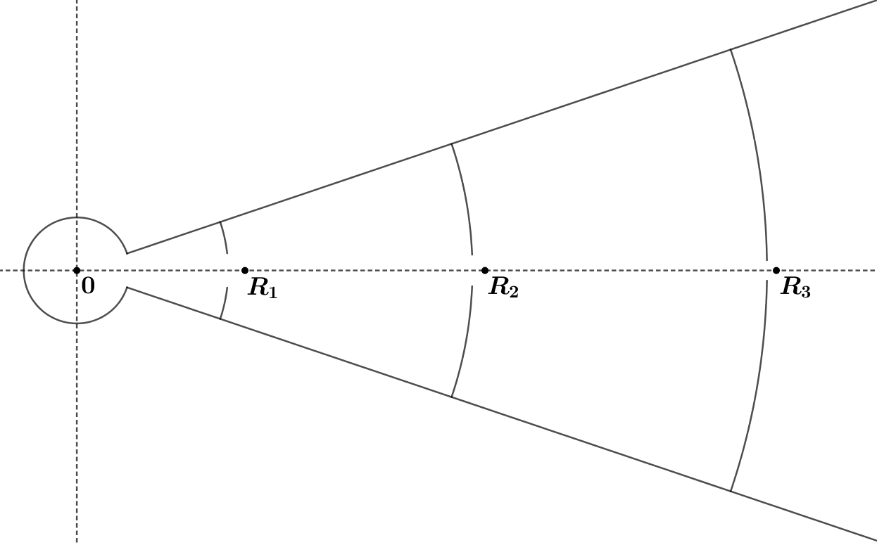
Figure 1.

In Section 3, we construct the simply connected domain $D$ of Fig. 1 and prove that there exists a sequence of positive numbers ${\left\{{{R_{n}}}\right\}_{n\in\mathbb{N}}}$ such that

$$\mathop{\lim}\limits_{n\to+\infty}\frac{{{{\hat{\omega}}_{D}}\left({{R_{n}}}\right)}}{{{\omega_{D}}\left({{R_{n}}}\right)}}=+\infty,$$

which implies that there does not exist a positive constant $C$ such that ${\omega_{D}}\left({R}\right)\geq C{{\hat{\omega}}_{D}}\left({R}\right)$ for every $R>0$. As we see in the proof, this result is due to the fact that the hyperbolic distance between the point $R_{n}$ and the hyperbolic geodesic, $\Gamma_{n}$, joining the endpoints of the arc $D\cap\left\{{\left|z\right|=R_{n}}\right\}$ in $D$ tends to infinity as $n\to+\infty$. In other words, there does not exist a positive constant $c$ such that $D\cap\left\{{\left|z\right|=R_{n}}\right\}\subset\left\{{z\in D:d_{D}\left({z,\Gamma_{n}}\right)<c}\right\}$ for every $n\in\mathbb{N}$. Note that $d_{D}\left({z,\Gamma_{n}}\right)$ denotes the hyperbolic distance between $z$ and $\Gamma_{n}$ in $D$, which we define in Section 2. Now we consider the following condition on the simply connected domain $D$:

Condition (1).

There exists a constant $c>0$ such that, for every $R>0$, every arc of $D\cap\left\{{z:\left|z\right|=R}\right\}$ lies in a hyperbolic $c$-neighborhood of the hyperbolic geodesic joining its endpoints.

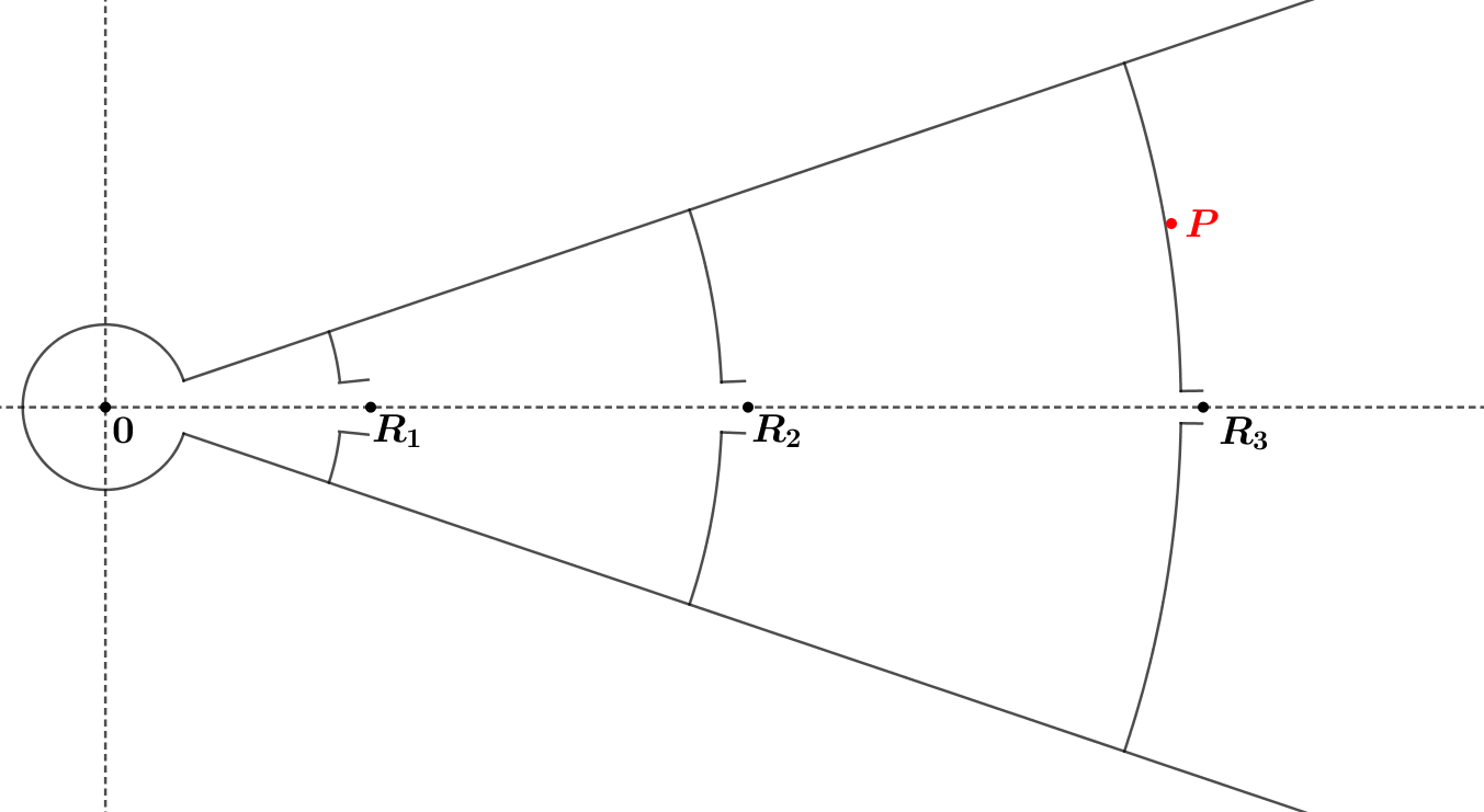
Figure 2.

The arising question is whether the answer to the Question 1.1 is positive for simply connected domains that satisfy Condition (1). However, we prove that this condition is not enough by constructing, in Section 4, the simply connected domain $D$ of Fig. 2, which comes from a small variation of the domain of Fig. 1. In fact, there exists a sequence of positive numbers ${\left\{{{R_{n}}}\right\}_{n\in\mathbb{N}}}$ such that, despite the fact that Condition (1) is satisfied, we have again

$$\mathop{\lim}\limits_{n\to+\infty}\frac{{{{\hat{\omega}}_{D}}\left({{R_{n}}}\right)}}{{{\omega_{D}}\left({{R_{n}}}\right)}}=+\infty.$$

This time, this is due to the fact that there exists a prime end $P$ of $\partial{D}$ that is inside the disk $\left\{{z:\left|z\right|<R_{n}}\right\}$ but every arc in $D$ joining $0$ to $P$ intersects the circle $\left\{{z:\left|z\right|=R_{n}}\right\}$. See, for example, the prime end $P$ in Fig. 2. So, we consider the following condition:

Condition (2).

For every $R>0$, there does not exist any prime end $P$ of $\partial{D}$ that is inside the disk $\left\{{z:\left|z\right|<R}\right\}$ but every arc in $D$ joining $0$ to $P$ intersects the circle $\left\{{z:\left|z\right|=R}\right\}$.

Note that in the first counter-example (Section 3) Condition (2) is satisfied, since it is obvious that there do not exist such prime ends. These two counter-examples show that Conditions (1) and (2) are necessary if we want to give a positive answer to the Question 1.1. But are they enough? In Section 5, we actually prove that if a simply connected domain satisfies Conditions (1) and (2), then there exists a positive constant $K=K\left(c\right)$ such that for every $R>0$,

$${{\hat{\omega}}_{D}}\left({R}\right)\leq K{\omega_{D}}\left({R}\right).$$

Moreover, we prove that we can find the value of this constant if we retain Condition (2) and replace Condition (1) with the following condition:

Condition (3).

For every $R>0$ and for every arc of $D\cap\left\{{z:\left|z\right|=R}\right\}$, the hyperbolic geodesic joining its endpoints lies entirely in $\overline{D}\cap\left\{{z:\left|z\right|\leq R}\right\}$.

So, having these results in mind, in Section 5, we prove the theorem below which gives a positive answer to the Question 1.1.

Theorem 1.1.

Let $D\subset\mathbb{C}$ be a simply connected domain with $0\in D$. With the notation above, if Conditions $\rm{(1)}$ and $\rm{(2)}$ are satisfied, then there exists a positive constant $K=K\left(c\right)$ such that for every $R>0$,

$${{\hat{\omega}}_{D}}\left({R}\right)\leq K{\omega_{D}}\left({R}\right).$$

If Conditions $\rm{(2)}$ and $\rm{(3)}$ are satisfied, then for every $R>0$,

$${{\hat{\omega}}_{D}}\left({R}\right)\leq 2{\omega_{D}}\left({R}\right).$$

Finally, recall that a domain $D$ in $\mathbb{C}$ is called starlike with respect to $0$, if for every point $z\in D$, the segment of the straight line from $0$ to $z$, $\left[{0,z}\right]$, lies entirely in $D$. In Section 6, we prove that starlike domains satisfy Conditions (2) and (3) and that $2$ is the optimal constant:

Theorem 1.2.

Let $D$ be a starlike domain in $\mathbb{C}$. Then for every $R>0$,

$${{\hat{\omega}}_{D}}\left({R}\right)\leq 2{\omega_{D}}\left({R}\right)$$

and the constant $2$ is best possible.

In Section 2, we introduce some preliminaries such as notions and results in hyperbolic geometry and basic properties of harmonic measure. In Sections 3 and 4, we present the counter-examples of Fig. 1 and 2 respectively, and in Sections 5 and 6, we prove Theorems 1.1 and 1.2 respectively.

2   Preliminary results

2.1   Results in hyperbolic geometry

For the unit disk $\mathbb{D}$ the density of the hyperbolic metric is

$${\lambda_{\mathbb{D}}}\left(z\right)=\frac{2}{{1-{{\left|z\right|}^{2}}}}.$$

Let $\Omega$ be a hyperbolic region in the complex plane $\mathbb{C}$; that is, $\mathbb{C}\backslash\Omega$ contains at least two points. If $f$ is a holomorphic universal covering projection of $\mathbb{D}$ onto $\Omega$ then the density $\lambda_{\Omega}$ is determined from

$${\lambda_{\Omega}}\left({f\left(z\right)}\right)\left|{f^{\prime}\left(z\right)}\right|=\frac{2}{{1-{{\left|z\right|}^{2}}}}$$

(see [Mi, p. 236]). The determination of $\lambda_{\Omega}$ is independent of the choice of the holomorphic covering projection onto $\Omega$. If $\Omega$ is simply connected, then $f$ is a conformal mapping of $\mathbb{D}$ onto $\Omega$. We note that in this paper we work on simlpy connected domains.

The hyperbolic distance between two points $z,w$ in $\mathbb{D}$ is defined by

$${d_{\mathbb{D}}}\left({z,w}\right)=\log\frac{{1+\left|{\frac{{z-w}}{{1-z\bar{w}}}}\right|}}{{1-\left|{\frac{{z-w}}{{1-z\bar{w}}}}\right|}}$$

(see [Ahl, ch. 1], [Bea, p. 11-28]). It is conformally invariant and thus it can be defined on any simply connected domain $D\neq\mathbb{C}$ as follows: If $f$ is a Riemann mapping of $\mathbb{D}$ onto $D$ and $z,w\in D$, then ${d_{D}}\left({z,w}\right)={d_{\mathbb{D}}}\left({{f^{-1}}\left(z\right),{f^{-1}}\left(w\right)}\right)$. Also, for a set $E\subset D$, we define ${d_{D}}\left({z,E}\right):=\inf\left\{{{d_{D}}\left({z,w}\right):w\in E}\right\}$.

The following theorem is known as Minda’s reflection principle [Mi, p. 241]. First, we introduce some notation: If $\Gamma$ is a straight line (or circle), then $R$ is one of the half-planes (or the disk) determined by $\Gamma$ and ${\Omega^{*}}$ is the reflection of a hyperbolic region $\Omega$ in $\Gamma$ .

Theorem 2.1.

Let $\Omega$ be a hyperbolic region in $\mathbb{C}$ and $\Gamma$ be a straight line or circle with $\Omega\cap\Gamma\neq\emptyset$. If $\Omega\backslash R\subset\Omega^{*}$, then

$${\lambda_{{\Omega^{*}}}}\left(z\right)\leq{\lambda_{\Omega}}\left(z\right)$$

for all $z\in\Omega\backslash\overline{R}$. Equality holds if and only if $\Omega$ is symmetric about $\Gamma$.

A generalization of Theorem 2.1 was proved by Solynin in [Sol].

2.2   Quasi-hyperbolic distance

The hyperbolic distance between $z_{1},z_{2}\in D$ can be estimated by the quasi-hyperbolic distance, ${\delta_{D}}\left({z_{1},z_{2}}\right)$, which is defined by

$${\delta_{D}}\left({{z_{1}},{z_{2}}}\right)=\mathop{\inf}\limits_{\gamma:{z_{1}}\to{z_{2}}}\int_{\gamma}{\frac{{\left|{dz}\right|}}{{d\left({z,\partial D}\right)}}},$$

where the infimum ranges over all the paths connecting $z_{1}$ to $z_{2}$ in $D$ and $d\left({z,\partial D}\right)$ denotes the Euclidean distance of $z$ from $\partial D$. Then it is proved that $\left({{1\mathord{\left/{\vphantom{12}}\right.\kern-1.2pt}2}}\right){\delta_{D}}\leq{d_{D}}\leq 2{\delta_{D}}$ (see [Bea, p. 33-36], [Co, p. 8]).

2.3   Harmonic measure

If $E\subset{{\overline{\mathbb{D}}\backslash\left\{0\right\}}}$, then a special case of the Beurling-Nevanlinna projection theorem (see [Ahl, p. 43-44], [Gar, p. 105] and [Ra, p. 120]) is the following:

Theorem 2.2.

Let $E\subset{{\overline{\mathbb{D}}\backslash\left\{0\right\}}}$ be a closed, connected set intersecting the unit circle. If ${r_{0}}=\min\left\{{\left|z\right|:z\in E}\right\}$ and ${E^{*}}=\left\{{-\left|z\right|:z\in E}\right\}=\left({-1,}\right.\left.{-{r_{0}}}\right]$, then

$${\omega_{\mathbb{D}}}\left({0,E}\right)\geq{\omega_{\mathbb{D}}}\left({0,{E^{*}}}\right)=\frac{2}{\pi}\arcsin\frac{{\left({1-{r_{0}}}\right)}}{{\left({1+{r_{0}}}\right)}}.$$

Next theorem states the strong Markov property for harmonic measure, which follows from the probabilistic interpretation of harmonic measure (see [Be, p. 282] and [Port, p. 88]).

Theorem 2.3.

Let $D_{1}$ and $D_{2}$ be two domains in $\mathbb{C}$. Assume that $D_{1}\subset{D_{2}}$ and let $F\subset\partial{D_{2}}$ be a closed set. If $\sigma=\partial{D_{1}}\backslash\partial{D_{2}}$, then for $z\in{D_{1}}$,

$${\omega_{{D_{2}}}}\left({z,F}\right)={\omega_{{D_{1}}}}\left({z,F}\right)+\int_{\sigma}{{\omega_{{D_{1}}}}\left({z,ds}\right){\omega_{{D_{2}}}}\left({s,F}\right)}.$$

The following result of Balogh and Bonk [Bo] gives an estimate of the logarithmic capacity of a set $E\subset\partial\mathbb{D}$. But this also proves an estimate of harmonic measure because if $E$ is a finite union of closed arcs in $\partial\mathbb{D}$, then $\omega_{\mathbb{D}}\left({0,E}\right)\leq{\rm cap}E$ (see [Gar, p. 164]).

Theorem 2.4.

There exists a universal constant $K>0$ with the following property. Suppose $f:\mathbb{D}\to\mathbb{C}$ is a conformal mapping with $\operatorname{dist}\left({f\left(0\right),\partial f\left(\mathbb{D}\right)}\right)\\ =d$. If $E_{f}\left(R\right)$ is the set of all $\zeta\in\partial\mathbb{D}$ with $\rm{length}$ $f\left({\left[{0,\zeta}\right)}\right)\geq R>0$, then

$${\rm cap}E_{f}\left(R\right)\leq K\sqrt{\frac{d}{R}}.$$

Next theorem states a relation between harmonic measure and hyperbolic distance, which we prove in [Kara].

Theorem 2.5.

Let $\Gamma$ be the hyperbolic geodesic joining two points $z_{1},z_{2}\in\partial{\mathbb{D}}$ in $\mathbb{D}$. Then

$${e^{-{d_{\mathbb{D}}}\left({0,\Gamma}\right)}}\leq{\omega_{\mathbb{D}}}\left({0,\Gamma}\right)\leq\frac{4}{\pi}{e^{-{d_{\mathbb{D}}}\left({0,\Gamma}\right)}}.$$

3   First counter-example

Hereinafter, we use the notation $D\left({z,r}\right):=\left\{{w\in\mathbb{C}:\left|{w-z}\right|<r}\right\}$ for some $z\in\mathbb{C}$ and some $r>0$. Let $D$ be the simply connected domain of Fig. 3, namely,

$$D=\mathbb{D}\cup\left(\left\{{z\in\mathbb{C}:\left|{\operatorname{Arg}{z}}\right|<1}\right\}\backslash\bigcup\limits_{n=1}^{+\infty}{\left\{{z\in\partial D\left({0,{e^{n}}}\right):\frac{1}{{{40^{n}}}}\leq\left|{\operatorname{Arg}{z}}\right|\leq 1}\right\}}\right)$$

and consider the sequence ${\left\{{{R_{n}}}\right\}_{n\in\mathbb{N}}}$ with ${R_{n}}={e^{n+\frac{1}{{{{40}^{n}}}}}}$ for every $n\in\mathbb{N}$.

Figure 3. The simply connected domain $D$.

Theorem 3.1.

With the notation above, the simply connected domain $D$ has the following properties:

1. $D$ satisfies Condition (2).

2. $D$ does not satisfy Condition (1).

3. $\mathop{\lim}\limits_{n\to+\infty}\frac{{{{\hat{\omega}}_{D}}\left({{R_{n}}}\right)}}{{{\omega_{D}}\left({{R_{n}}}\right)}}=+\infty.$

Proof.

Property (i) is immediate by the construction of $D$. So, we prove properties (ii) and (iii) (for a similar calculation see [Ka]). The Riemann mapping theorem implies that there exists a conformal mapping $\psi$ from $\mathbb{D}$ onto $D$ such that $\psi\left(0\right)=0$. For $n\in\mathbb{N}$, we set ${F_{R_{n}}}=\left\{{z\in\mathbb{D}:\left|{\psi\left(z\right)}\right|={R_{n}}}\right\}$ and ${E_{R_{n}}}=\left\{{\zeta\in\partial\mathbb{D}:\left|{\psi\left(\zeta\right)}\right|\geq{R_{n}}}\right\}$. Also, for $n\in\mathbb{N}$, let $\Gamma_{R_{n}}$ be the hyperbolic geodesic joining the endpoints of $F_{{R_{n}}}$ in $\mathbb{D}$.

By Theorem 2.2 and the definition of hyperbolic distance we can easily infer that for every $n\in\mathbb{N}$,

$${\omega_{\mathbb{D}}}\left({0,{F_{R_{n}}}}\right)\geq\frac{2}{\pi}{e^{-{d_{\mathbb{D}}}\left({0,{F_{R_{n}}}}\right)}}$$

(see [Co, p. 35]). So, by the conformal invariance of harmonic measure and hyperbolic distance, we have

(3.1) $$\hat{\omega}_{D}\left({R_{n}}\right)=\omega_{D}\left({0,\psi\left({F_{R_{n}}}\right)}\right)\geq\frac{2}{\pi}e^{-d_{D}\left({0,\psi\left({F_{R_{n}}}\right)}\right)}.$$

Now fix a number $n>2$. If $z\in D$ and ${g_{D}}\left({\cdot,\cdot}\right)$ denotes the Green function for $D$ (see [Gar, p. 41-43], [Ra, p. 106-115]), then

$${d_{D}}\left(0,z\right)=\log\frac{{1+{e^{-{g_{D}}\left({0,z}\right)}}}}{{1-{e^{-{g_{D}}\left({0,z}\right)}}}}$$

(see [Bea, p. 12-13] and [Ra, p. 106]). For every $w_{n}\in\psi\left({{F_{{R_{n}}}}}\right)\backslash\left\{{{R_{n}}}\right\}$ (see Fig. 4), we infer, by a symmetrization result, that

$${g_{D}}\left({0,{R_{n}}}\right)\geq{g_{D}}\left({0,w_{n}}\right)$$

(see Lemma 9.4 in [Hay, p. 659]). Since

$$f\left(x\right)=\log\frac{{1+{e^{-x}}}}{{1-{e^{-x}}}}$$

is a decreasing function on $\left({0,+\infty}\right)$, we have that

$${d_{D}}\left({0,\psi\left({{F_{{R_{n}}}}}\right)}\right)={d_{D}}\left({0,{R_{n}}}\right).$$

This in conjunction with (3.1) implies that

(3.2) $$\hat{\omega}_{D}\left({R_{n}}\right)\geq\frac{2}{\pi}e^{-d_{D}\left({0,R_{n}}\right)}.$$

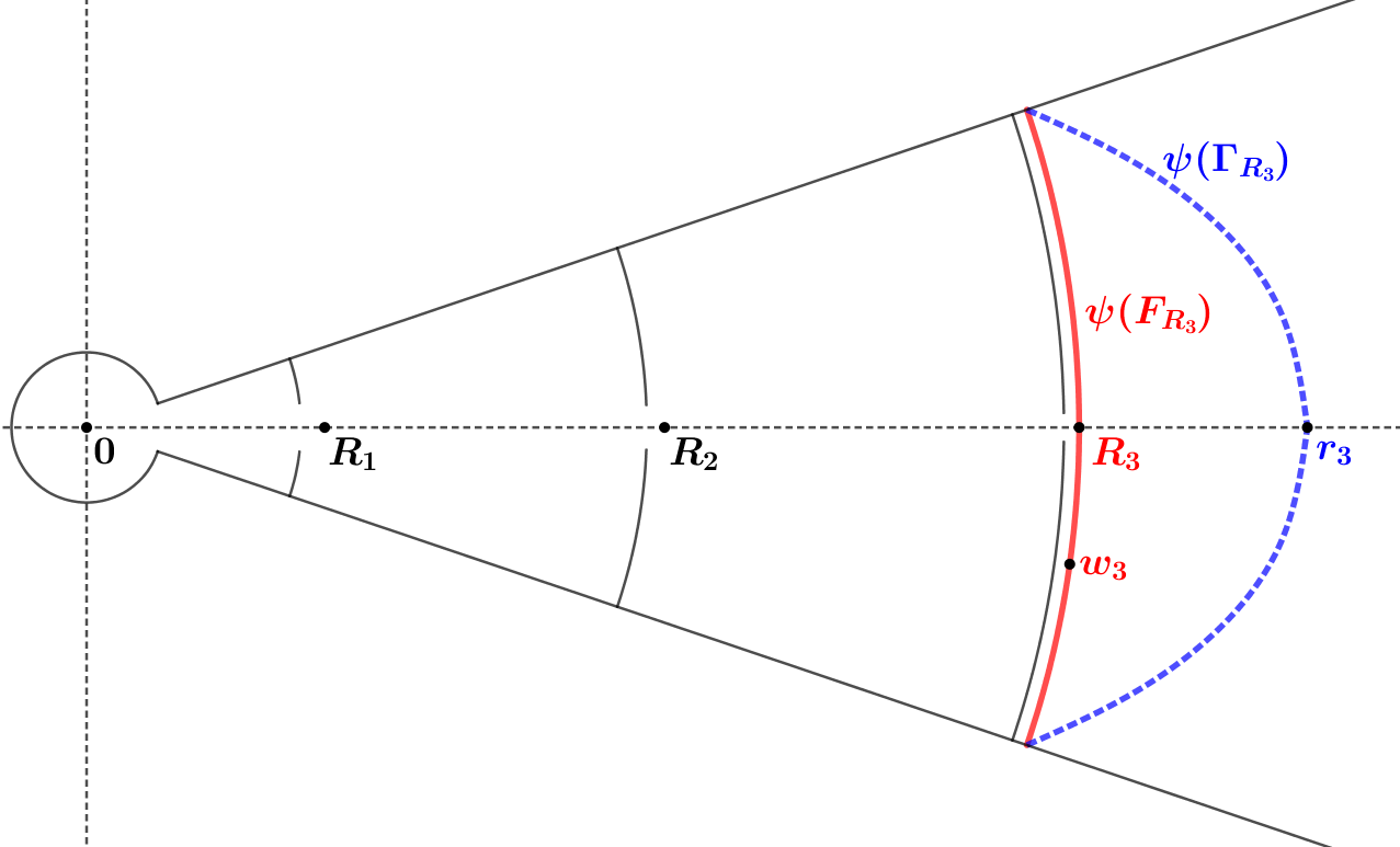
Figure 4. The crosscuts $\psi\left({{F_{{R_{n}}}}}\right)$ and $\psi\left({{\Gamma_{{R_{n}}}}}\right)$ in case $n=3$.

Since ${\Gamma_{{R_{n}}}}$ denotes the hyperbolic geodesic joining the endpoints of $F_{{R_{n}}}$ in $\mathbb{D}$, by Theorem 2.5 and [Beu, p. 370],

$${\omega_{\mathbb{D}}}\left({0,{E_{{R_{n}}}}}\right)=\frac{1}{2}{\omega_{\mathbb{D}}}\left({0,{\Gamma_{{R_{n}}}}}\right)\leq\frac{2}{\pi}{e^{-{d_{\mathbb{D}}}\left({0,{\Gamma_{{R_{n}}}}}\right)}}$$

and thus

(3.3) $$\omega_{D}\left({R_{n}}\right)=\omega_{D}\left({0,\psi\left({E_{R_{n}}}\right)}\right)\leq\frac{2}{\pi}e^{-d_{D}\left({0,\psi\left({\Gamma_{R_{n}}}\right)}\right)}.$$

Since $D$ is symmetric with respect to the real axis, we deduce that

$${d_{D}}\left({{0},\psi\left({{\Gamma_{{R_{n}}}}}\right)}\right)={d_{D}}\left({0,{r_{n}}}\right),$$

where ${r_{n}}=\psi\left({{\Gamma_{{R_{n}}}}}\right)\cap\mathbb{R}\in\left({e^{n},e^{n+1}}\right)$ (see Fig. 4) and hence by (3.3) we conclude that

(3.4) $$\omega_{D}\left({R_{n}}\right)\leq\frac{2}{\pi}e^{-d_{D}\left(0,r_{n}\right)}.$$

Since $0,\,R_{n}$ and $r_{n}$ lie, in this order, along a hyperbolic geodesic (for more details see [Ka]), we have that

$${d_{D}}\left({0,{r_{n}}}\right)={d_{D}}\left({0,{R_{n}}}\right)+{d_{D}}\left({{R_{n}},{r_{n}}}\right)$$

(see [Bea, p. 14]). Combining this with (3.2) and (3.4), we deduce that

(3.5) $$\frac{{\hat{\omega}_{D}\left({R_{n}}\right)}}{{\omega_{D}\left({R_{n}}\right)}}\geq e^{d_{D}\left({0,r_{n}}\right)-d_{D}\left({0,R_{n}}\right)}=e^{d_{D}\left({R_{n},r_{n}}\right)}.$$

Now notice that the quasi-hyperbolic distance (see Section 2) $\delta_{D}\left({R_{n},r_{n}}\right)$ is equal to $\delta_{D\backslash{\overline{\mathbb{D}}}}\left({R_{n},r_{n}}\right)$ because the quasi-hyperbolic geodesic joining $R_{n}$ to $r_{n}$ in $D$ and the quasi-hyperbolic geodesic joining $R_{n}$ to $r_{n}$ in $D\backslash{\overline{\mathbb{D}}}$ is the segment $\left[{R_{n},r_{n}}\right]$ in both cases. So, we deduce that

(3.6) $$d_{D}\left({R_{n},r_{n}}\right)\geq\frac{1}{2}\delta_{D}\left({R_{n},r_{n}}\right)=\frac{1}{2}\delta_{D\backslash{\overline{\mathbb{D}}}}\left({R_{n},r_{n}}\right)\geq\frac{1}{4}d_{D\backslash{\overline{\mathbb{D}}}}\left({R_{n},r_{n}}\right).$$

In order to simplify our computations we use the conformal mapping $g\left(z\right)=\operatorname{Log}z$ that maps $D\backslash\overline{\mathbb{D}}$ onto $g\left({D\backslash\overline{\mathbb{D}}}\right):=D^{\prime}$ (see Fig. 5).

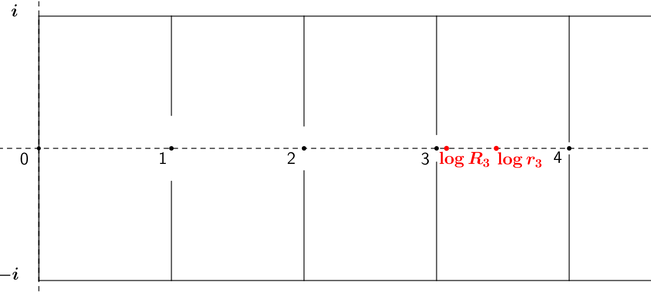
Figure 5. The domain $D^{\prime}$ and the points $\log R_{n}$, $\log r_{n}$ in case $n=3$.

Thus, we get

(3.7) $$d_{D\backslash{\overline{\mathbb{D}}}}\left({R_{n},r_{n}}\right) = {d_{D^{\prime}}}\left({\log R_{n},\log r_{n}}\right)\geq\frac{1}{2}{\delta_{D^{\prime}}}\left(\log R_{n},\log r_{n}\right)$$

$$= \frac{1}{2}\int_{{{\mathop{\log R_{n}}}}}^{\log r_{n}}{\frac{{dx}}{{d\left({x,\partial D^{\prime}}\right)}}}\geq\frac{1}{2}\int_{\log R_{n}}^{\log r_{n}}{\frac{{dx}}{{\sqrt{{{\left({\frac{1}{{{40^{n}}}}}\right)}^{2}}+{{\left({x-n}\right)}^{2}}}}}}$$

$$= \frac{1}{2}\operatorname{arcsinh}\left({{40^{n}}\left({\log r_{n}-n}\right)}\right)-\frac{1}{2}\operatorname{arcsinh}\left({1}\right)$$

$$\geq \frac{1}{2}\operatorname{arcsinh}\left({{40^{n}}k}\right)-\frac{1}{2}\operatorname{arcsinh}\left({1}\right),$$

where $k>0$ is a constant independent of $n$ (see [Ka]). Now, taking limits in (3.7) as $n\to+\infty$, we obtain

$$\mathop{\lim}\limits_{n\to+\infty}d_{D\backslash{\overline{\mathbb{D}}}}\left({R_{n},r_{n}}\right)=+\infty.$$

Thus, by (3.6) we conclude that

(3.8) $$\mathop{\lim}\limits_{n\to+\infty}d_{D}\left({R_{n},r_{n}}\right)=+\infty,$$

which proves property (ii). Finally, by (3.5) and (3.8), we infer that

$$\mathop{\lim}\limits_{n\to+\infty}\frac{{{{\hat{\omega}}_{D}}\left({{R_{n}}}\right)}}{{{\omega_{D}}\left({{R_{n}}}\right)}}=+\infty$$

and hence property (iii) holds. So, there does not exist a positive constant $C$ such that for every $R>0$,

$${\omega_{D}}\left({R}\right)\geq C{{\hat{\omega}}_{D}}\left({R}\right).$$

∎

4   Second counter-example

Let $D$ be the simply connected domain of Fig. 6, namely,

$$D=\mathbb{D}\cup\left(\left\{{z\in\mathbb{C}:\left|{\operatorname{Arg}{z}}\right|<1}\right\}\backslash{D_{0}}\right),$$

where

$$D_{0} =\bigcup_{n=1}^{+\infty}\bigg{(}\left\{z\in\partial D(0,e^{n}):\frac{1}{40^{n}}\leq|\operatorname{Arg}z|\leq 1\right\}$$

$$\quad\quad\quad\qquad\cup\left\{re^{i\theta}:e^{n}\leq r\leq e^{n+1/40^{n}},\,|\theta|=\frac{1}{40^{n}}\right\}\bigg{)}.$$

We consider the sequence ${\left\{{{R_{n}}}\right\}_{n\in\mathbb{N}}}$ with ${R_{n}}={e^{n+1/40^{n}}}$ for every $n\in\mathbb{N}$.

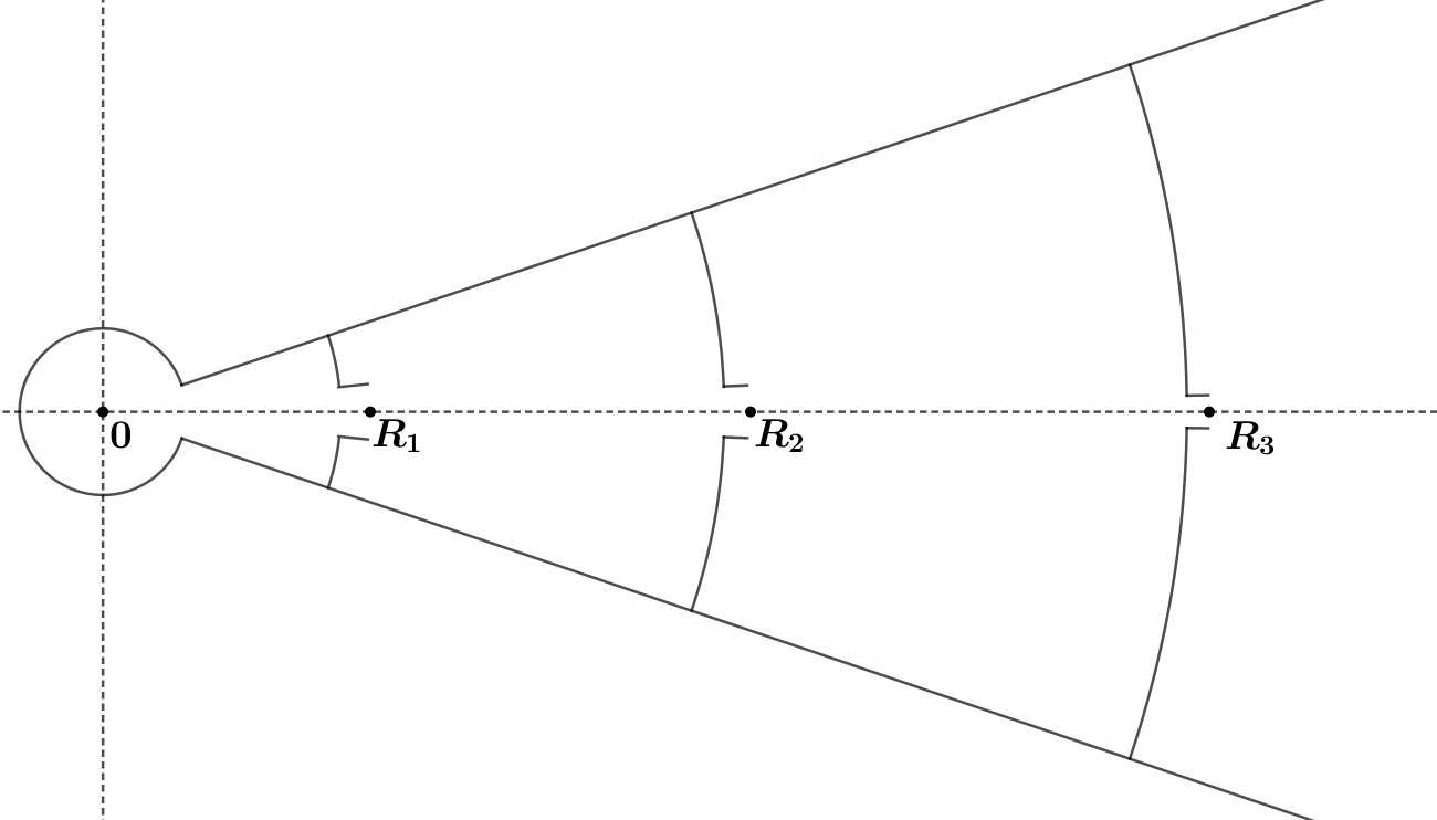
Figure 6. The simply connected domain $D$.

Theorem 4.1.

With the notation above, the simply connected domain $D$ has the following properties:

1. $D$ does not satisfy Condition (2).

2. $D$ satisfies Condition (1).

3. $\mathop{\lim}\limits_{n\to+\infty}\frac{{{{\hat{\omega}}_{D}}\left({{R_{n}}}\right)}}{{{\omega_{D}}\left({{R_{n}}}\right)}}=+\infty.$

Proof.

Property (i) is immediate by the construction of $D$. So, we prove properties (ii) and (iii). First we introduce some notation. For $n\in\mathbb{N}$, let ${F_{R_{n}}}$ be the component of $D\cap\left\{{\left|z\right|=R_{n}}\right\}$ that intersects the real axis and $\Gamma_{R_{n}}$ be the hyperbolic geodesic joining the endpoints of $F_{R_{n}}$ in $D$. Also, we set ${E_{R_{n}}}=\partial D\cap\left\{{\left|z\right|\geq R_{n}}\right\}$ for every $n\in\mathbb{N}$.

Now we apply Jørgensen’s theorem [Jo, p. 116] that a Euclidean disk inside a simply connected domain is hyperbolically convex. Combining this with the construction of $D$, we deduce that, for every $n\in\mathbb{N}$, we can find a disk $D_{n}\subset D$ centered at a point of $\mathbb{R}$ (see Fig. 7) that satisfies the following properties:

1. $D_{n}$ contains the arc ${F_{R_{n}}}$ and the geodesic $\Gamma_{R_{n}}$.

2. The endpoints of ${F_{R_{n}}}$ lie on $\partial D_{n}$.

3. The Euclidean distance of each point of $\partial D_{n}$ from $\partial D$ is attained on the set $\left\{re^{i\theta}:e^{n}\leq r\leq e^{n+1/40^{n}},\,|\theta|=\frac{1}{40^{n}}\right\}$.

4. If $\theta_{n}$ is the acute angle between $\left\{re^{i\theta}:e^{n}\leq r\leq e^{n+1/40^{n}},\,\theta=\frac{1}{40^{n}}\right\}$ and the tangent of $\partial D_{n}$ at the point $z_{n}=e^{n+1/40^{n}}e^{1/40^{n}i}$, then $\theta_{n}\geq k$ for some constant $k>0$ independent of $n$ (see Fig. 7).

So, if $s\in D_{n}\cap\left\{{z:{\mathop{\rm Im}\nolimits}z\geq 0}\right\}$ then we can easily infer that

(4.1) $$\operatorname{dist}\left({s,\partial D}\right)=\left|{s-z_{n}}\right|\,\,{\rm or}\,\,\operatorname{dist}\left({s,\partial D}\right)\geq\sin k\left|{s-z_{n}}\right|.$$

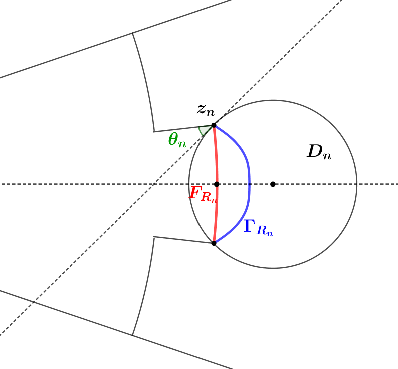
Figure 7.

Since $D$ and $D_{n}$ are symmetric with respect to $\mathbb{R}$, (4.1) also holds for every $s\in D_{n}\cap\left\{{z:{\mathop{\rm Im}\nolimits}z<0}\right\}$ by replacing $z_{n}$ with ${\bar{z}_{n}}$. So, (4.1) in combination with the fact that $F_{R_{n}},\Gamma_{R_{n}}$ lie in $D_{n}$ and join $z_{n}$ to ${\bar{z}_{n}}$ implies that, for every $n\in\mathbb{N}$, the quasi-hyperbolic distance between any point of $F_{R_{n}}$ and $\Gamma_{R_{n}}$ is bounded from above by an absolute positive constant. Thus, the hyperbolic distance between any point of $F_{R_{n}}$ and $\Gamma_{R_{n}}$ is bounded from above by an absolute positive constant. This proves property (ii).

Now set $L_{n}=\operatorname{dist}\left({R_{n},\left\{{z\in\mathbb{C}:\left|{\operatorname{Arg}z}\right|=1}\right\}}\right)$ and $d_{n}=\operatorname{dist}\left({R_{n},\partial D}\right)$. By the construction of $D$, there exists a number $n_{0}\in\mathbb{N}$ such that for every $n>n_{0}$ and every $s\in F_{R_{n}}$ (see Fig. 8),

$$D\left({s,\frac{{L_{n}}}{2}}\right)\subset\left\{{z\in\mathbb{C}:\left|{\operatorname{Arg}z}\right|<1}\right\}\,\,\,{\rm and}\,\,\,D\left({s,\frac{{L_{n}}}{2}}\right)\cap E_{R_{n}}=\emptyset.$$

Fix a number $n>n_{0}$ and a point $s\in F_{R_{n}}$. The Riemann mapping theorem implies that there exists a conformal mapping $f$ from $\mathbb{D}$ onto $D$ such that $f\left(0\right)=s$. Therefore, applying Theorem 2.4 with its notation, we have that

(4.2) $$\omega_{D}\left({s,E_{R_{n}}}\right) = \omega_{\mathbb{D}}\left({0,f^{-1}\left({E_{R_{n}}}\right)}\right)\leq{\rm cap}f^{-1}\left({E_{R_{n}}}\right)\leq{\rm cap}E_{f}\left({\frac{{L_{n}}}{2}}\right)$$

$$\leq K\sqrt{\frac{{2d_{s}}}{{L_{n}}}}\leq K\sqrt{\frac{{2d_{n}}}{{L_{n}}}},$$

where $d_{s}=\operatorname{dist}\left({s,\partial D}\right)$. So, by Theorem 2.3 and relation (4.2), we infer that for every $n>n_{0}$,

$$\frac{{\hat{\omega}_{D}\left({R_{n}}\right)}}{{\omega_{D}\left({R_{n}}\right)}}=\frac{{\omega_{D}\left({0,F_{R_{n}}}\right)}}{{\omega_{D}\left({0,E_{R_{n}}}\right)}}=\frac{{\omega_{D}\left({0,F_{R_{n}}}\right)}}{{\int_{F_{R_{n}}}{\omega_{D}\left({0,ds}\right)\omega_{D}\left({s,E_{R_{n}}}\right)}}}\geq\frac{1}{K}\sqrt{\frac{{L_{n}}}{{2d_{n}}}}.$$

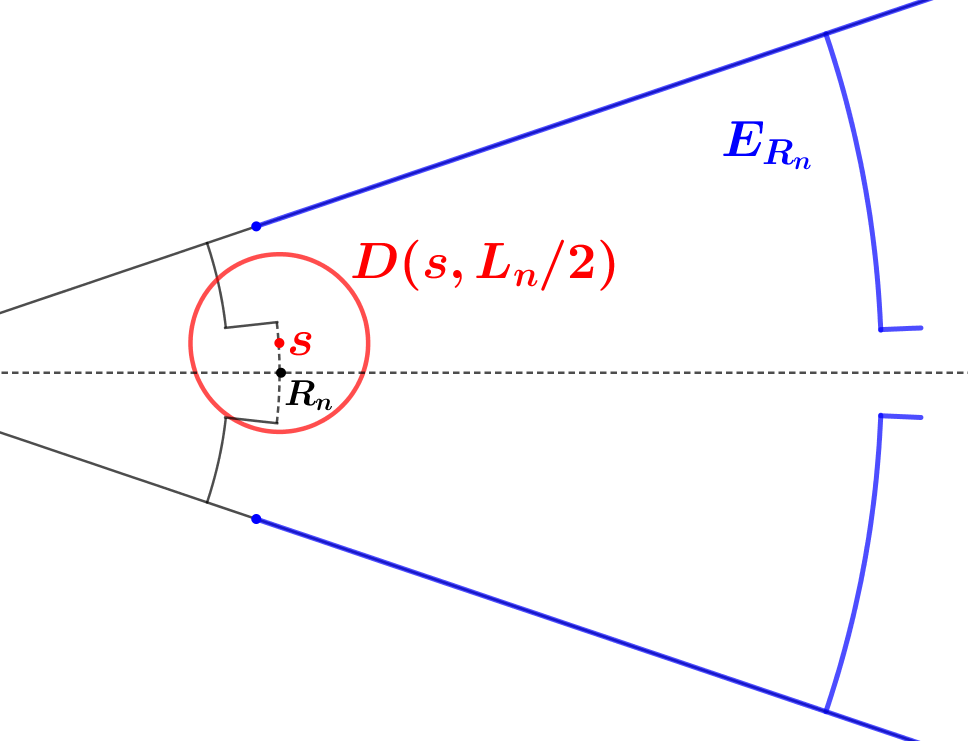
Figure 8.

Taking limits as $n\to+\infty$, we deduce that

$$\mathop{\lim}\limits_{n\to+\infty}\frac{1}{K}\sqrt{\frac{{L_{n}}}{{2d_{n}}}}=+\infty$$

and hence

$$\mathop{\lim}\limits_{n\to+\infty}\frac{{\hat{\omega}_{D}\left({R_{n}}\right)}}{{\omega_{D}\left({R_{n}}\right)}}=+\infty.$$

This proves property (iii).

∎

5   Proof of theorem 1.1

Proof of Theorem 1.1.

Since $D$ is a simply connected domain, the Riemann mapping theorem implies that there exists a conformal mapping $\psi$ from $\mathbb{D}$ onto $D$ with $\psi\left(0\right)=0$. Now we introduce some notation. For $R>0$, we set ${F_{R}}=\left\{{z\in\mathbb{D}:\left|{\psi\left(z\right)}\right|=R}\right\}$, that is, $\psi\left({{F_{R}}}\right)=D\cap\left\{{z:\left|z\right|=R}\right\}$. Note that since $\psi\left({{F_{R}}}\right)$ is a countable union of open arcs in $D$ that are the intersection of $D$ with the circle $\left\{{z:\left|z\right|=R}\right\}$, the preimage of every such arc is also an arc in $\mathbb{D}$ with two distinct endpoints on $\partial\mathbb{D}$ (see Proposition 2.14 [Pom, p. 29]). Also, let $N\left(R\right)\in\mathbb{N}\cup\left\{{+\infty}\right\}$ denote the number of components of $F_{R}$ and

$$I_{R}=\left\{\begin{array}[]{l}\left\{{1,2,\ldots,N\left(R\right)}\right\},\,{\rm{if}}\,N\left(R\right)<+\infty\\ \mathbb{N},\,\,\,\,\,\,\,\,\,\,\,\,\,\,\,\,\,\,\,\,\,\,\,\,\,\,\,\,\,\,\,\,\,\,\,\,\,\,\,\,\,{\rm{if}}\,N\left(R\right)=+\infty\\ \end{array}\right..$$

If ${\left\{{F_{R}^{i}}\right\}_{i\in I_{R}}}$ are the components of $F_{R}$, then, for every $i\in I_{R}$, we set ${\Gamma}_{R}^{i}$ be the hyperbolic geodesic joining the endpoints of $F_{R}^{i}$ in $\mathbb{D}$ and $C_{R}^{i}$ be the arc of $\partial\mathbb{D}$ joining the endpoints of ${\Gamma}_{R}^{i}$ and lying on the boundary of the component of $\mathbb{D}\backslash{{\Gamma}_{R}^{i}}$ which does not contain the origin (see Fig. 10).

Suppose that Conditions (2) and (3) are satisfied. For every $R>0$ and $i\in I_{R}$ and for each $z\in{{\Gamma}_{R}^{i}}$, we have that

$${\omega_{\mathbb{D}}}\left({z,C_{R}^{i}}\right)=\frac{1}{2},$$

(see [Beu, p. 370]). Condition (3) implies that each crosscut $F_{R}^{i}$ is contained in the component of $\mathbb{D}\backslash{{\Gamma}_{R}^{i}}$ bounded by ${{\Gamma}_{R}^{i}}$ and $C_{R}^{i}$ (see Fig. 10). Thus, by the maximum principle, we deduce that for every $z\in{F_{R}^{i}}$,

(5.1) $${\omega_{\mathbb{D}}}\left({z,C_{R}^{i}}\right)\geq\frac{1}{2}.$$

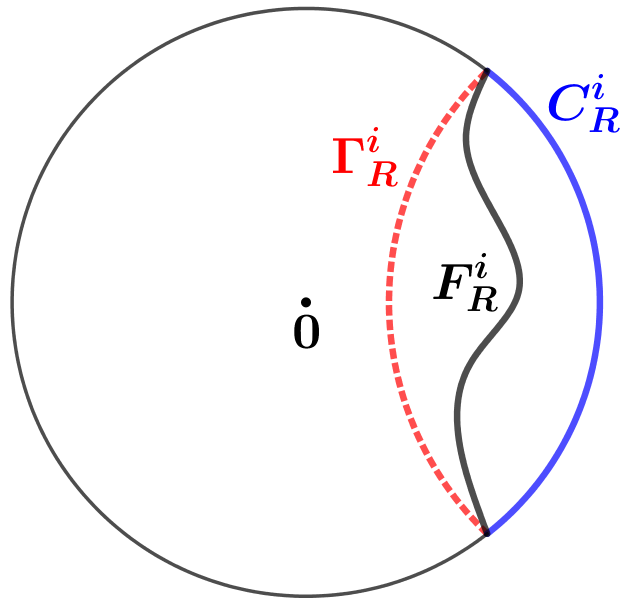
Figure 9.

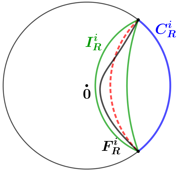
Figure 10.

Applying Theorem 2.3 and relation (5.1), we infer that

(5.2) $$\omega_{\mathbb{D}}\left({0,C_{R}^{i}}\right) = \int\limits_{F_{R}^{i}}{\omega_{\mathbb{D}}\left({0,dz}\right)\omega_{\mathbb{D}}\left({z,C_{R}^{i}}\right)}\geq\frac{1}{2}\int\limits_{F_{R}^{i}}{\omega_{\mathbb{D}}\left({0,dz}\right)}$$

$$= \frac{1}{2}\omega_{\mathbb{D}}\left({0,F_{R}^{i}}\right)$$

for every $R>0$ and every $i\in I_{R}$. Condition (2) and the conformal invariance of harmonic measure imply that

$$\omega_{D}\left(R\right)\geq\omega_{\mathbb{D}}\left({0,\bigcup\limits_{i\in I_{R}}{C_{R}^{i}}}\right)=\sum\limits_{i\in I_{R}}{\omega_{\mathbb{D}}\left({0,C_{R}^{i}}\right)}.$$

Combining this with (5.2) we get

$$\omega_{D}\left(R\right) \geq \sum\limits_{i\in I_{R}}{\omega_{\mathbb{D}}\left({0,C_{R}^{i}}\right)}\geq\frac{1}{2}\sum\limits_{i\in I_{R}}{\omega_{\mathbb{D}}\left({0,F_{R}^{i}}\right)}=\frac{1}{2}\omega_{\mathbb{D}}\left({0,\bigcup\limits_{i\in I_{R}}{F_{R}^{i}}}\right)$$

$$= \frac{1}{2}\omega_{\mathbb{D}}\left({0,{F_{R}}}\right)=\frac{1}{2}\omega_{D}\left({0,\psi\left({F_{R}}\right)}\right)=\frac{1}{2}\hat{\omega}_{D}\left(R\right)$$

and thus we have the desired result

$${{\hat{\omega}}_{D}}\left({R}\right)\leq 2{\omega_{D}}\left({R}\right)$$

for every $R>0$.

Now suppose that Conditions (1) and (2) are satisfied. By Condition (1) we infer that, for every $R>0$ and every $i\in I_{R}$, there exists a hyperbolic $k_{c}$-neighborhood, $U_{R}^{i}$, of ${{\Gamma}_{R}^{i}}$ such that $\partial{U_{R}^{i}}$ consists of two circular arcs in $\mathbb{D}$ and ${F_{R}^{i}}$ is contained in $U_{R}^{i}$ (see Fig. 10). Note that $k_{c}$ is a positive constant that depends only on $c$. Let ${I_{R}^{i}}$ denote the circular arc of $\partial{U_{R}^{i}}$ such that ${F_{R}^{i}}$ is contained in the component of $\mathbb{D}\backslash{I_{R}^{i}}$ bounded by ${I_{R}^{i}}$ and $C_{R}^{i}$ (see Fig. 10). For every $R>0$ and $i\in I_{R}$ and for each $z\in{I_{R}^{i}}$, we have that

$${\omega_{\mathbb{D}}}\left({z,C_{R}^{i}}\right)=k^{\prime},$$

where $k^{\prime}$ lies in the open interval $\left(0,1\right)$ and depends only on $k_{c}$ and hence only on $c$. Now we repeat the argument above letting ${I_{R}^{i}}$ play the role of ${{\Gamma}_{R}^{i}}$. Therefore, for every $z\in{F_{R}^{i}}$,

(5.3) $${\omega_{\mathbb{D}}}\left({z,C_{R}^{i}}\right)\geq k^{\prime}.$$

By Theorem 2.3 and relation (5.3), we infer that

$$\omega_{\mathbb{D}}\left({0,C_{R}^{i}}\right)=\int\limits_{F_{R}^{i}}{\omega_{\mathbb{D}}\left({0,dz}\right)\omega_{\mathbb{D}}\left({z,C_{R}^{i}}\right)}\geq k^{\prime}\omega_{\mathbb{D}}\left({0,F_{R}^{i}}\right)$$

for every $R>0$ and every $i\in I_{R}$. This in conjunction with Condition (2) implies that

$$\omega_{D}\left(R\right) \geq \omega_{\mathbb{D}}\left({0,\bigcup\limits_{i\in I_{R}}{C_{R}^{i}}}\right)=\sum\limits_{i\in I_{R}}{\omega_{\mathbb{D}}\left({0,C_{R}^{i}}\right)}\geq k^{\prime}\sum\limits_{i\in I_{R}}{\omega_{\mathbb{D}}\left({0,F_{R}^{i}}\right)}$$

$$= k^{\prime}\omega_{\mathbb{D}}\left({0,{F_{R}}}\right)=k^{\prime}\hat{\omega}_{D}\left(R\right).$$

So, we conclude that for every $R>0$,

$${{\hat{\omega}}_{D}}\left({R}\right)\leq K{\omega_{D}}\left({R}\right),$$

where $K=\frac{1}{{k^{\prime}}}$ is a positive constant that depends only on $c$.

∎

6   Proof of theorem 1.2

In the proof of Theorem 1.2 we will use the following result which is an easy computation coming from the conformal invariance of harmonic measure.

Lemma 6.1.

Let $a\in\left({0,1}\right)$ and $b\in\left[{0,1}\right)$. Then

$${\omega_{\mathbb{D}\backslash\left[{a,1}\right)}}\left({-b,\partial{\mathbb{D}}}\right)=1-\frac{2}{\pi}\arctan\frac{1}{{\sqrt{{{\left({\frac{{\left({1+a}\right)\left({1+b}\right)}}{{\left({1-a}\right)\left({1-b}\right)}}}\right)}^{2}}-1}}}.$$

Proof of Theorem 1.2.

Let $D$ be a starlike domain in $\mathbb{C}$. Using the notation of the proof of Theorem 1.1, we will prove that Conditions (2) and (3) are satisfied. Since $D$ is starlike, Condition (2) is obviously satisfied and thus we prove Condition (3). Let ${F_{R}^{i}}$ be a component of $F_{R}$ for some $i\in I_{R}$. Suppose that $\psi\left({\Gamma_{R}^{i}}\right)\not\subset\overline{D}\cap\left\{{z:\left|z\right|\leq R}\right\}$, then $\psi\left({\Gamma_{R}^{i}}\right)$ contains a curve ${\gamma_{R}^{i}}$ lying in $D\backslash D\left({0,R}\right)$ with endpoints $z_{1},z_{2}\in\partial{D\left({0,R}\right)}$ (see Fig. 11). Since $\psi\left({\Gamma_{R}^{i}}\right)$ is the hyperbolic geodesic joining the endpoints of $\psi\left({F_{R}^{i}}\right)$ in $D$, ${\gamma_{R}^{i}}$ is the hyperbolic geodesic joining $z_{1}$ to ${z_{2}}$ in $D$. Notice that $D$ is a hyperbolic region in $\mathbb{C}$ such that $D\cap\partial D\left({0,R}\right)\neq\emptyset$. Since $D$ is starlike, we have that $D\backslash D\left({0,R}\right)\subset D^{*}$, where $D^{*}$ is the reflection of $D$ in the circle $\partial D\left({0,R}\right)$. So, applying Theorem 2.1, we get

$${\lambda_{{D^{*}}}}\left(z\right)<{\lambda_{D}}\left(z\right),\;z\in{\gamma_{R}^{i}}$$

and thus

$$\int_{{{\gamma_{R}^{i}}}^{*}}{{\lambda_{D}}\left({{z^{*}}}\right)\left|{d{z^{*}}}\right|}<\int_{{\gamma_{R}^{i}}}{{\lambda_{D}}\left(z\right)\left|{dz}\right|},$$

where ${{\gamma_{R}^{i}}}^{*}$ is the reflection of ${\gamma_{R}^{i}}$ in $\partial D\left({0,R}\right)$. But this leads to contradiction because ${\gamma_{R}^{i}}$ is the hyperbolic geodesic joining $z_{1}$ to ${z_{2}}$ in $D$. So, $\psi\left({\Gamma_{R}^{i}}\right)\subset\overline{D}\cap\left\{{z:\left|z\right|\leq R}\right\}$ and thus Condition (3) is satisfied. Theorem 1.1 implies that for every $R>0$,

$${{\hat{\omega}}_{D}}\left({R}\right)\leq 2{\omega_{D}}\left({R}\right).$$

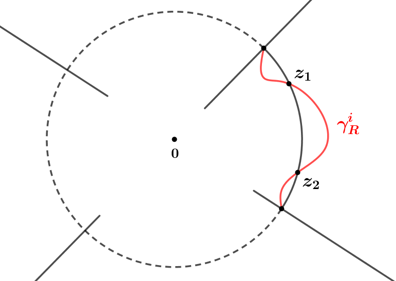
Figure 11.

Now we prove that the constant $2$ is best possible. Consider the Koebe function $K\left(z\right)=\frac{z}{{{{\left({1-z}\right)}^{2}}}}$ which maps $\mathbb{D}$ conformally onto $D_{0}:=\mathbb{C}\backslash\left({-\infty,-\frac{1}{4}}\right]$. For $R>{\frac{1}{4}}$, by the conformal invariance of harmonic measure and Lemma 6.1, we have

(6.1) $${{\hat{\omega}}_{D_{0}}}\left({R}\right) = {\omega_{D\left({0,R}\right)\backslash\left({-R,-\frac{1}{4}}\right]}}\left({0,\partial D\left({0,R}\right)}\right)={\omega_{\mathbb{D}\backslash\left({-1,-\frac{1}{{4R}}}\right]}}\left({0,\partial\mathbb{D}}\right)$$

$$= {\omega_{\mathbb{D}\backslash\left[{\frac{1}{{4R}},1}\right)}}\left({0,\partial\mathbb{D}}\right)=1-\frac{2}{\pi}\arctan\frac{1}{{\sqrt{{{\left({\frac{{4R+1}}{{4R-1}}}\right)}^{2}}-1}}}$$

$$= 1-\frac{2}{\pi}\arctan\frac{{4R-1}}{{4\sqrt{R}}}.$$

Using the fact that

$${K^{-1}}\left({-R}\right)=\left({\frac{{2R-1}}{{2R}}}\right)\pm i\frac{{\sqrt{4R-1}}}{{2R}}$$

and the conformal invariance of harmonic measure, we deduce that

(6.2) $${{\omega}_{D_{0}}}\left({R}\right) = {\omega_{D_{0}}}\left({0,\left({-\infty,-R}\right]}\right)$$

$$= {\omega_{\mathbb{D}}}\left({0,\operatorname{arc}\left({\left({\frac{{2R-1}}{{2R}}}\right)-i\frac{{\sqrt{4R-1}}}{{2R}},\left({\frac{{2R-1}}{{2R}}}\right)+i\frac{{\sqrt{4R-1}}}{{2R}}}\right)}\right)$$

$$= 2{\omega_{\mathbb{D}}}\left({0,\operatorname{arc}\left({1,\left({\frac{{2R-1}}{{2R}}}\right)+i\frac{{\sqrt{4R-1}}}{{2R}}}\right)}\right)$$

$$= \frac{1}{\pi}\arctan\frac{{\sqrt{4R-1}}}{{2R-1}},$$

where $\operatorname{arc}\left({\left({\frac{{2R-1}}{{2R}}}\right)-i\frac{{\sqrt{4R-1}}}{{2R}},\left({\frac{{2R-1}}{{2R}}}\right)+i\frac{{\sqrt{4R-1}}}{{2R}}}\right)$ denotes the arc of $\partial\mathbb{D}$ joining $\left({\frac{{2R-1}}{{2R}}}\right)-i\frac{{\sqrt{4R-1}}}{{2R}}$ to $\left({\frac{{2R-1}}{{2R}}}\right)+i\frac{{\sqrt{4R-1}}}{{2R}}$ counterclockwise. Applying (6.1) and (6.2), we infer that

$$\mathop{\lim}\limits_{R\to+\infty}\frac{{{{\hat{\omega}}_{D_{0}}}\left({R}\right)}}{{{\omega_{D_{0}}}\left({R}\right)}}=\mathop{\lim}\limits_{R\to+\infty}\frac{{\pi-2\arctan\frac{{4R-1}}{{4\sqrt{R}}}}}{{\arctan\frac{{\sqrt{4R-1}}}{{2R-1}}}}=2.$$

Suppose that there exists a positive constant $C<2$ such that for every starlike domain $D$ and every $R>0$, ${{\hat{\omega}}_{D}}\left({R}\right)\leq C{\omega_{D}}\left({R}\right)$. This implies for $D_{0}$ that

$$2=\mathop{\lim}\limits_{R\to+\infty}\frac{{{{\hat{\omega}}_{{D_{0}}}}\left({R}\right)}}{{{\omega_{{D_{0}}}}\left({R}\right)}}\leq C,$$

which leads to contradiction. Therefore, the constant $2$ is best possible.

∎

Note that we could also prove Theorem 1.2 by using instead of Minda’s reflection principle and Theorem 1.1, the strong Markov property for harmonic measure (see Section 2).

Another proof of Theorem 1.2.

Let $D$ be a starlike domain in $\mathbb{C}$. Set ${F_{R}}=D\cap\partial D\left({0,R}\right)$, ${E_{R}}=\partial D\backslash D\left({0,R}\right)$, ${L_{R}}=\partial D\cap D\left({0,R}\right)$ and ${D_{0}}=D\cap D\left({0,R}\right)$ as illustrated in Fig. 12. So, we have the relations

(6.3) $${{\hat{\omega}}_{D}}\left({R}\right)={\omega_{{D_{0}}}}\left({0,{F_{R}}}\right)=1-{\omega_{{D_{0}}}}\left({0,{L_{R}}}\right)$$

and

(6.4) $${\omega_{D}}\left({R}\right)={\omega_{D}}\left({0,{E_{R}}}\right)=1-{\omega_{D}}\left({0,{L_{R}}}\right).$$

Figure 12. The starlike domain $D$.

By Theorem 2.3,

$${\omega_{D}}\left({0,{L_{R}}}\right)={\omega_{{D_{0}}}}\left({0,{L_{R}}}\right)+\int_{{F_{R}}}{{\omega_{{D_{0}}}}\left({0,ds}\right){\omega_{D}}\left({s,{L_{R}}}\right)}$$

which in conjunction with (6.3) and (6.4) implies that

(6.5) $${{\hat{\omega}}_{D}}\left({R}\right)={\omega_{D}}\left({R}\right)+\int_{{F_{R}}}{{\omega_{{D_{0}}}}\left({0,ds}\right){\omega_{D}}\left({s,{L_{R}}}\right)}.$$

Let $N\left(R\right)\in\mathbb{N}\cup\left\{{+\infty}\right\}$ denote the number of components of ${F_{R}}$ and

$$I_{R}=\left\{\begin{array}[]{l}\left\{{1,2,\ldots,N\left(R\right)}\right\},\,{\rm{if}}\,N\left(R\right)<+\infty\\ \mathbb{N},\,\,\,\,\,\,\,\,\,\,\,\,\,\,\,\,\,\,\,\,\,\,\,\,\,\,\,\,\,\,\,\,\,\,\,\,\,\,\,\,\,{\rm{if}}\,N\left(R\right)=+\infty\\ \end{array}\right..$$

If ${\left\{{F_{R}^{i}}\right\}_{i\in I_{R}}}$ are the components of $F_{R}$, then

(6.6) $$\int_{{F_{R}}}{{\omega_{{D_{0}}}}\left({0,ds}\right){\omega_{D}}\left({s,{L_{R}}}\right)}=\sum\limits_{i\in I_{R}}{\int_{F_{R}^{i}}{{\omega_{{D_{0}}}}\left({0,ds}\right){\omega_{D}}\left({s,{L_{R}}}\right)}},$$

since ${F_{R}^{i}}$ are mutually disjoint sets.

Now let ${F_{R}^{i}}$ be a component of $F_{R}$ for some $i\in I_{R}$. If $z_{1},z_{2}$ denote the endpoints of ${F_{R}^{i}}$ such that $\operatorname{Arg}{z_{1}}<\operatorname{Arg}{z_{2}}$, then we set

$$L_{R}^{*}=\left\{{r{e^{i\operatorname{Arg}{z_{1}}}}:0\leq r\leq R}\right\}\cup\left\{{r{e^{i\operatorname{Arg}{z_{2}}}}:0\leq r\leq R}\right\}$$

and

$${D^{*}}=\left\{{z\in\mathbb{C}:\operatorname{Arg}{z_{1}}<\operatorname{Arg}z<\operatorname{Arg}{z_{2}}}\right\}$$

as illustrated in Fig. 13. For every $s\in F_{R}^{i}$,

(6.7) $${\omega_{D}}\left({s,{L_{R}}}\right)\leq{\omega_{{D^{*}}}}\left({s,L_{R}^{*}}\right).$$

Figure 13.

If $\theta=\operatorname{Arg}{z_{2}}-\operatorname{Arg}{z_{1}}$, we consider the conformal mappings

$${f_{1}}\left(z\right)=z{e^{-i\left({\operatorname{Arg}{z_{2}}-{\theta\mathord{\left/{\vphantom{\theta 2}}\right.\kern-1.2pt}2}}\right)}},\,{f_{2}}\left(z\right)={z^{{\pi\mathord{\left/{\vphantom{\pi\theta}}\right.\kern-1.2pt}\theta}}},\,{f_{3}}\left(z\right)=\frac{{z-1}}{{z+1}}.$$

Then the composition $f={f_{3}}\circ{f_{2}}\circ{f_{1}}$ maps $D^{*}$ conformally onto $\mathbb{D}$. Since $f\left({F_{R}^{i}}\right)$ is the hyperbolic geodesic joining $f\left({{z_{1}}}\right)$ to $f\left({{z_{2}}}\right)$ in $\mathbb{D}$, for every $s\in F_{R}^{i}$,

$${\omega_{{D^{*}}}}\left({s,L_{R}^{*}}\right)={\omega_{\mathbb{D}}}\left({f\left(s\right),f\left({L_{R}^{*}}\right)}\right)=\frac{1}{2}.$$

This in combination with (6.7) implies that for every $s\in F_{R}^{i}$,

$${\omega_{D}}\left({s,{L_{R}}}\right)\leq\frac{1}{2}.$$

By this and relations (6.5) and (6.6) we infer that

$${{\hat{\omega}}_{D}}\left({R}\right) = {\omega_{D}}\left({R}\right)+\sum\limits_{i\in I_{R}}{\int_{F_{R}^{i}}{{\omega_{{D_{0}}}}\left({0,ds}\right){\omega_{D}}\left({s,{L_{R}}}\right)}}$$

$$\leq {\omega_{D}}\left({R}\right)+\frac{1}{2}\sum\limits_{i\in I_{R}}{\int_{F_{R}^{i}}{{\omega_{{D_{0}}}}\left({0,ds}\right)}}$$

$$= {\omega_{D}}\left({R}\right)+\frac{1}{2}\sum\limits_{i\in I_{R}}{\omega_{{D_{0}}}}\left({0,F_{R}^{i}}\right)={\omega_{D}}\left({R}\right)+\frac{1}{2}{\omega_{{D_{0}}}}\left({0,{F_{R}}}\right)$$

$$= {\omega_{D}}\left({R}\right)+\frac{1}{2}{{\hat{\omega}}_{D}}\left({R}\right),$$

and thus for every $R>0$,

$${{\hat{\omega}}_{D}}\left(R\right)\leq 2{\omega_{D}}\left(R\right).$$

The fact that the constant $2$ is best possible is proved as before.

∎