Sparse, Low-bias, and Scalable Estimation of High Dimensional Vector Autoregressive Models via Union of Intersections

Abstract

Vector autoregressive ($VAR$) models are widely used for causal discovery and forecasting in multivariate time series analyses in fields as diverse as neuroscience, environmental science, and econometrics. In the high-dimensional setting, model parameters are typically estimated by $L_{1}$-regularized maximum likelihood; yet, when applied to $VAR$ models, this technique produces a sizable trade-off between sparsity and bias with the choice of the regularization hyperparameter, and thus between causal discovery and prediction. That is, low-bias estimation entails dense parameter selection, and sparse selection entails increased bias; the former is useful in forecasting but less likely to yield scientific insight leading to discovery of causal influences, and conversely for the latter. This paper presents a scalable algorithm for simultaneous low-bias and low-variance estimation (hence good prediction) with sparse selection for high-dimensional $VAR$ models. The method leverages the recently developed Union of Intersections ($UoI$) algorithmic framework for flexible, modular, and scalable feature selection and estimation that allows control of false discovery and false omission in feature selection while maintaining low bias and low variance. This paper demonstrates the superior performance of the $UoI_{VAR}$ algorithm compared with other methods in simulation studies, exhibits its application in data analysis, and illustrates its good algorithmic scalability in multi-node distributed memory implementations.

1 Introduction

Temporal multivariate data are now ubiquitous across scientific fields and increasingly high-dimensional. Data dimensionalities are growing rapidly with advancing measurement technologies [37], which presents opportunities for scientific discovery alongside methodological and computational challenges for data analysis. Examples of multivariate time-series data are numerous across different scientific fields. In neuroscience, for instance, electrophysiology produces simultaneous recordings of neural activity as measured by large arrays of hundreds to thousands of electrodes sampling on rapid timescales ranging from 4kHz to 30kHz [15] and further. Data with analogous structure is generated in neuroscience from electroencephalography (EEG) [2], functional magnetic resonance imaging (fMRI) [30], local field potentials (LFP) [19], and various other sources [12, 38, 6]. In econometrics and fincance, temporal multivariate data is used for forecasting, macroeconomic studies, and structural analysis [40, 20, 22, 42, 45]. Similar data are arising on increasing scales in environmental science and geosciences [29], epidemiology [16], and sociology [35]. These data pose challenges alongside promise for discovery.

Many research questions motivating the collection and analysis of temporal multivariate data pertain to characterizing dependence between component time series: climate scientists conduct attribution studies relating global temperatures to changing atmospheric conditions and human activity [43]; neuroscientists approximate functional networks of neural sites active under certain experimental conditions [38]. Thus, multivariate time series data can be collected to understand structure among the components of a single system, or to study mutual influences between several interacting systems. Modeling techniques that address these questions and are applicable to large data sets are therefore both needed and potentially impact many areas given the breadth of disciplines collecting such data.

Standard multivariate time series analysis techniques use parametric Gaussian process models for forecasting, structural analysis (finding a unique process parametrization under ‘structural’ constraints), impulse response analysis (describing the propagation of a ‘shock’ or erratic event throughout the system), and estimation of various types of causality; vector autoregressive ($VAR$) models provide a flexible framework for these tasks and are probabilistically tractable and computationally straightforward to estimate [34], though scaling to massive systems is a challange.

Vector autoregressive models are particularly well-suited to causal discovery. In $VAR$ models, each mean parameter links one lagged component time series with one non-lagged series at some order of temporal offset; this process parametrization yields the property that forecasting error (specifically mean square error of optimal predictors of a certain class) is nondecreasing under exclusion of lagged univariate series linked by nonzero parameters to the rest of the system [34]. That property is given a causal interpretation wherein one time series is said to be causal for another if information about the former improves forecasting of the latter. This effect of reducing forecasting error is referred to as Granger causality [25, 17, 4, 1].

Granger-causal graphical modeling of large datasets requires high-dimensional process models, for which $VAR$ parameters are often estimated with sparsity constraints. This paradigm for causal discovery requires scalable methods with good statistical properties, and has motivated statistical research in sparse estimation of high-dimensional autoregressive models [41, 21, 28, 39, 7, 27]. Interesting sparsity constraints also arise in related literature on joint estimation of multiple Gaussian graphical models [26, 18].

Sparse estimation methods for time series models rely on $L_{1}$-regularized likelihood estimation (LASSO regularization). However, in high-dimensional regression and precision matrix estimation this technique can result in overfitting and excessive bias [14, 36] with high false positive rates. While post-hoc thresholding of estimated couplings can be applied to sparsify graphs, these ad hoc approaches resist rigorous mathematical analysis and are often set by analysts to achieve preconceived notions of graph structure. Many of these problems appear to be exacerbated by the additional structure present in time series data, and to date, few alternatives to LASSO regularization are available in time series analysis for high-dimensional data. These statistical challenges can potentially change scientific interpretation about data generation processes. Union of Intersections ($UoI$) is a recently-introduced algorithmic framework for sparse, low-bias and low-variance estimation in statistical models that results in improved predictive accuracy [8]. The framework is flexible, modular, and scalable, and enhances both the identification of features (model selection) as well as the estimation of the contributions of these features (model estimation) to data generation processes, thereby leading to improved interpretability and prediction [8]. At their core, $UoI$-based methods leverage data resampling (bootstraping) and a range of sparsity-inducing regularization strengths to efficiently build families of potential model features, and separate model feature selection with intersection operations from model parameter estimation with union operations [8].

Given the intensive use of resampling methods in the $UoI$ algorithmic framework, bootstrap procedures suitable for time series are required to create a $UoI$-based method for $VAR$ models. One of the most common bootstrap procedures for time series is the moving block bootstrap [32, 33], in which the original time series is divided into overlapping blocks and the blocks are randomly sampled with replacement to construct a resampling of the original time series [31]. The choice of appropriate block lengths is dependent on the statistical problem [13, 31].

This paper offers a two-fold contribution to the above-cited work: (i) an inference procedure that improves on $L_{1}$-regularized estimation of high-dimensional vector autoregressive models leveraging the Union of Intersections ($UoI$) algorithmic framework [8]; and (ii) provision of simulation-based and theoretical support for the algorithm, techniques producing good scalability, and a data analysis application demonstrating the use of the method. While this work focuses on Gaussian $VAR$ models, the method is generalizable to a much broader class of parametric models with autoregressive structure [27].

The paper is organized as follows. Methods (Section 2) provides background on the Gaussian $VAR$ model class and algorithmic framework before presenting the $UoI_{VAR}$ algorithm. Results (Section 3) illustrates the method’s performance in a simulation study, demonstrates its application in an analysis of equity share price data, discusses computational runtime analyses of the algorithm under strong and weak scaling. Theory (Section 4) provides some consistency results of simplified $UoI_{VAR}$ estimator. The paper closes with a discussion of the modularity of the method, practical challenges encountered in the course of its development, and potential extensions of this research.

2 Methods

2.1 Multivariate Autoregressions

Gaussian vector autoregressive processes of order $D$ ($VAR(D)$) refer to the parametric family of stochastic processes characterized by

$$X_{t}=\nu+\sum_{d=1}^{D}A_{d}X_{t-d}+\epsilon_{t}\;,\quad\epsilon_{t}\stackrel{{\scriptstyle iid}}{{\sim}}N(0,\bm{\Sigma})$$ (1)

for all $t\in\mathbb{Z}$ where $\bm{\Sigma}\in\mathbb{R}^{M\times M}$ is positive definite and $A_{1},\dots,A_{D}$ satisfy $\text{det}\left(\bm{I}-\sum_{d=1}^{D}\bm{A}_{d}z^{d}\right)\neq 0$ for all $|z|\leq 1$. The latter condition ensures that the process is well-defined, stationary and stable. $M$ is the process dimension.

For $VAR(D)$ processes, Granger causality is defined with reference to the minimal-$MSE$ $h$-step predictor of the process from time $t$. Let $z(X_{t+h}|X_{t})$ be the optimal (minimum $MSE$) $h$-step predictor of $X_{t+h}$ given $X_{t}$, and partition $X_{t}=(X_{t}^{A},X_{t}^{B})$; then the subprocess $X_{t}^{A}$ Granger-causes the subprocess $X_{t}^{B}$ just in case for at least one $h$,

$$MSE\left(z(X_{t+h}^{B}|X_{t}^{B})\right)\geq MSE\left(z(X_{t+h}^{B}|X_{t}^{A},X_{t}^{B})\right)$$

If $X_{t}^{A}$ and $X_{t}^{B}$ are univariate subprocesses in positions $i$ and $j$ respectively, Granger causality is equivalent to the condition that $(A_{d})_{ij}\neq 0$ for at least one $d$. Instantaneous causality is a similar property expressible in terms of entries of $\bm{\Sigma}_{-1}$; for a precise definition and further discussion, refer to [34].

A $VAR(D)$ model is a $VAR(D)$ process stipulated as the data-generating process for an observed vector time series of length $T$, denoted $\{X_{t}\in\mathbb{R}^{M}\}_{t=0}^{T}$. The model can be expressed in the form of a multivariate multiple regression $\bm{Y}=\bm{UB}+\bm{E}$ where $\bm{Y}=(X_{T}\;X_{T-1}\;\cdots\;X_{D})^{T}$ comprises the observations beginning from time $D$, the error terms are, similarly, $\bm{E}=(\epsilon_{T}\;\epsilon_{T-1}\;\cdots\;\epsilon_{D})^{T}$, and the linear predictor $\bm{UB}$ on the right-hand side is

$$\left(\begin{array}[]{c:c:c:c}1&X_{T-1}^{T}&\cdots&X_{T-D}^{T}\\ 1&X_{T-2}^{T}&\cdots&X_{T-D-1}^{T}\\ \vdots&\vdots&\ddots&\vdots\\ 1&X_{D-1}^{T}&\cdots&X_{0}^{T}\\ \end{array}\right)\left(\begin{array}[]{c}\nu^{T}\\ A_{1}^{T}\\ \vdots\\ A_{D}^{T}\end{array}\right)$$ (2)

The classical model estimation technique is to estimate the mean parameter $\bm{B}$ with ordinary least squares (OLS), i.e., as $\hat{\bm{B}}=(\bm{U}^{\prime}\bm{U})^{-1}\bm{U}^{\prime}\bm{Y}$, and then estimate the covariance matrix $\bm{\Sigma}$ with $\hat{\bm{\Sigma}}=\frac{1}{T-1}(\bm{Y}-\bm{U\hat{B}})(\bm{Y}-\bm{U\hat{B}})^{\prime}$; the equivalence of this procedure with maximum likelihood (ML) estimation is well-established [34].

When $M$ is large and $A_{1},\dots,A_{D}$ are sparse, the standard estimation technique is $L_{1}$-regularized maximum likelihood, i.e., solving the optimization problem

$$\arg\min_{\bm{B}}\left\{-\ell(\bm{B};\bm{X})+\lambda P(\bm{B})\right\}$$ (3)

where $\ell(\bm{B};\bm{X})$ denotes the log-likelihood of the matrix parameter $\bm{B}$ given data $\bm{X}=(X_{1}\cdots X_{T})\in\mathbb{R}^{M\times T}$, and $P(\bm{B})=\|\text{vec}\bm{B}\|_{1}$ is the regularization term. Due to the equivalence between ML and OLS, $\|\bm{Y}-\bm{UB}\|_{F}^{2}$ can be substituted for $-\ell(\bm{B};\bm{X})$ in Equation (3) and LASSO regression on the vectorized problem (column-stacking the response $\bm{Y}$ for a univariate regression formulation) can be used to find the solution with fast, numerically stable, and widely available algorithms [23, 24].

2.2 Union of Intersections

The Union of Intersections algorithmic framework separates sparse feature selection (‘Intersection’) from parameter estimation (‘Union’). Its advantages over base methods are established for several sparse learning techniques, including regression and classification [8], and matrix decomposition [8, 46]. The framework is modular, employs data resampling and bootstrap aggregation, and is conducive to algorithmic parallelism, and has hyperparameters that modulate forces toward sparser or denser selection while maintaining low bias and low variance estimates. Specifically, in the ‘Intersection step’, UoI first infers a set of candidate parameter supports through intersection operations across bootstrap samples for a range of sparsity-inducing regularization ranges. Then, in the ‘Union step’, OLS estimates are calculated for each candidate support on a separate bootstrap samples and model fit predictive quality is evaluated on a separate sample. Finally, the estimates that optimize predictive quality are averaged (a unionizing operation) to produce the final model output.

2.3 $UoI_{VAR}$ Algorithm

The $UoI_{VAR}$ algorithm builds the base LASSO estimation method (Equation (3)) into the $UoI$ framework. The intersection step and union step of $UoI_{VAR}$ are given separately as Algorithms 1 and 2; $UoI_{VAR}$ refers to the composite of both algorithms performed in sequence.

Algorithm 1 Intersection step

0:  

  data $\{X_{t}\in\mathbb{R}^{M}\}_{t=0}^{T}$

  regularization path $\lambda\in\mathbb{R}^{K}$

  number of bootstrap samples $B_{1}$

  bootstrap block length $L$

  thresholding parameter $s$

  for $b=1$ to $B_{1}$ do

     draw bootstrap sample $\{X_{t}^{*}\}_{t=0}^{T}$ 

     for $k=1$ to $K$ do

        $\tilde{\bm{B}}_{k}\leftarrow\arg\min_{\bm{B}}\left\{-\ell(\bm{B}\;;\;\bm{X}^{*})+\lambda_{k}P(\bm{B})\right\}$

        $S_{b,k}\leftarrow\{(i,j):\;\tilde{b}_{ij}\neq 0\}$

     end for

  end for

  $S_{k}\leftarrow\left\{(i,j):\;\sum_{b=1}^{B_{1}}\mathbbm{1}\{(i,j)\in S_{b,k}\}\geq sB_{1}\right\}$

  Support sets $S_{1},\dots,S_{k}$

The first step is in essence a relaxation of the bootstrapped LASSO [3] carried out only to the point of support sets, that is, without returning an estimate. In this step, for a fixed regularization path $\lambda$, LASSO supports (sets of nonzero parameter locations) are computed for $B_{1}$ bootstrap samples and then aggregated for each $\lambda_{k}$ by a thresholded intersection operation. Algorithm 1 selects consistently recurring support sets under resampling of the data $B_{1}$ times, with a specifiable recurrence threshhold $s$.

Algorithm 2 Union step

0:  

  data $\{X_{t}\in\mathbb{R}^{M}\}_{t=0}^{T}$

  support sets $S_{1},\dots,S_{K}$

  number of bootstrap samples $B_{2}$

  bootstrap block length $L$

  fit metric $f$

  for $b=1$ to $B_{2}$ do

     draw bootstrap sample $\{X_{t}^{*(1)}\}_{t=0}^{T}$

     draw bootstrap sample $\{X_{t}^{*(2)}\}_{t=0}^{T}$

     for $k=1$ to $K$ do

        $\mathcal{B}\leftarrow\left\{\bm{B}\in\mathbb{R}^{(D+1)\times M}:b_{ij}=b_{ij}\mathbbm{1}\{(i,j)\in S_{k}\}\right\}$

        $\tilde{\bm{B}}_{k}\leftarrow\arg\min_{\bm{B}\in\mathcal{B}}\left\{-\ell(\bm{B}\;;\;\bm{X}^{*(1)})\right\}$

        $f_{k}\leftarrow f(\tilde{\bm{B}}_{k};\bm{X}^{*(2)})$

     end for

     $\hat{\bm{B}}^{(b)}\leftarrow\tilde{\bm{B}}_{J}:J=\arg\min_{k}\{f_{k}\}$

  end for

  $\bm{\hat{B}}\leftarrow\frac{1}{B_{2}}\sum_{b=1}^{B_{2}}\hat{\bm{B}}^{(b)}$ 

  UoI estimate $\hat{\bm{B}}$

The second step performs bagging [11] by cross-validation with bootstrap samples to choose support sets and estimation parameters by OLS. In this step, for $B_{2}$ iterations, training and test bootstrap samples are drawn, OLS estimates are computed for each support set from the intersection step, and the estimate that gives best fit on the test set is stored; then, the $B_{2}$ estimates are averaged to give the $UoI_{VAR}$ estimate. Algorithm 2 averages predictively accurate unbiased estimates under resampling of the data $B_{2}$ times.

The hyperparameters $B_{1}$, $B_{2}$, and $s$ balance sparsity and predictive accuracy, and can be manipulated to achieve pressure toward either direction: increasing $B_{1}$ produces greater sparsity, decreasing $s$ creates less sparsity, and doing both simultaneously controls for stochastic exclusion of desirable parameters due to erratic bootstrap samples; increasing $B_{2}$ improves predictions but increases density.

3 Theory

This section analyzes a simplified version of the $UoI_{VAR}$ estimator of the transition matrices $A_{1},\ldots,A_{d}$ defined in Equation (1). In place of a theoretical analysis of the $UoI_{VAR}$ algorithm in its full generality as presented in Section 2.3, the following concentrates on the intersection step only (Algorithm 1), although in closing known results which can be suitably modified to demonstrate the theoretical validity of the union step (Algorithm 2) are indicated.

Let data $\{X_{t}\in\mathbb{R}^{M}\}_{t=0}^{T}$ be generated from a Gaussian vector autoregressive process of order $D$ ($VAR(D)$); then $\{X_{t}\in\mathbb{R}^{M}\}_{t=0}^{T}$ is a vector time-series dimension $M$. The data-generating equation can be written in the form

$$\bm{Y}_{N\times M}=\bm{U}_{N\times(DM+1)}\bm{B}_{(DM+1)\times M}+\bm{E}_{N\times M},$$ (4)

where, $N=(T-D+1)$ per Equation (2). Equation (4) can be vectorized as

$$\mathcal{Y}_{NM\times 1}=\mathcal{X}_{NM\times q}\bm{\beta}_{q\times 1}+\text{vec}(\bm{E})_{NM\times 1},$$ (5)

where $\mathcal{Y}=\text{vec}(\bm{Y})$, $\mathcal{X}=(\text{I}\otimes\bm{U})$, $\bm{\beta}=\text{vec}(\bm{B})$ and $q=M(DM+1)$. Let $\bm{\beta}^{*}$ be the unknown fixed parameter and assume it is $s$-sparse, that is, $||\bm{\beta}^{*}||_{0}=s$.

Note that by hypothesis the data-generating process is stable: $\text{det}\left(\bm{I}-\mathcal{A}(z)\right)\neq 0$ on the unit circle of the complex plane $\{z\in\mathbb{C}:|z|=1\}$, where $\mathcal{A}(z)=\sum_{d=1}^{D}\bm{A}_{d}z^{d}$. Note also that control of the eigenstructure of $\mathcal{A}(z)$ is given by $\mu_{min}(\mathcal{A}):=\min_{|z|=1}\Lambda_{min}(\mathcal{A}^{*}(z)\mathcal{A}(z))$ and $\mu_{max}(\mathcal{A}):=\Lambda_{max}(\mathcal{A}^{*}(z)\mathcal{A}(z))$. $\Lambda_{max}(A)$ and $\Lambda_{min}(A)$ are the mean maximum and minimum eigenvalue of the matrix $A$, and $A^{*}$ is the conjugate of $A$.

For ease of theoretical analysis, consider a special case of Algorithm 1, where the threshold parameter is set to $s=1$, so that the algorithm performs strict intersection of the support sets from different bootstrap samples. In fact, $s=1$ is a decent default value in practice. Although the validity of Algorithm 1 is only proven in estimating support sets of $A_{1},\ldots,A_{d}$ for $s=1$, the argument can be extended from this special case with some additional effort to $s\in(0,1]$, which is left for future work.

In Algorithm 1, bootstrap samples are drawn from the multivariate time-series $\{X_{t}\in\mathbb{R}^{M}\}_{t=0}^{T}$ using the moving block bootstrap (MBB) method [32, 33]. The MBB method resamples blocks randomly with replacement from the subcollection $\{\mathcal{B}(i,k):i=1,\ldots,T-L+1,k=L\}$ of overlapping blocks, where $\mathcal{B}(i,k)$ is a block of size $k$ containing observations from time steps $t=i,\ldots,i+k-1$. Let $I_{1},\ldots,I_{b}$ be conditionally $iid$ random variables with the discrete uniform distribution on $\{1,\ldots,T-L+1\}$, that is, $\mathbb{P}(I_{1}=i)=(T-L+1)^{-1}$, $1<i<T-L+1$, where $b=T/L$. Thus, the resampled blocks for the MBB are given by $\mathcal{B}(I_{1},L),\ldots,\mathcal{B}(I_{b},L)$ and arranging the elements in all $b$ blocks in a sequence. The result is the bootstrap sample $\{\mathbf{X}^{*}_{1},\ldots,\mathbf{X}^{*}_{L},\mathbf{X}^{*}_{L+1},\ldots,\mathbf{X}^{*}_{2L},\ldots,\mathbf{X}^{*}_{bL}\}$.

Now consider the estimation part of Algorithm 1, wherein the estimation problem is stated as $\tilde{\bm{B}}_{k}=\arg\min_{\bm{B}}\left\{-\ell(\bm{B}\;;\;\bm{X}^{*})+\lambda_{k}P(\bm{B})\right\}$. For the present purpose the functional form for $\ell(\bm{B}\;;\;\bm{X})$ is fixed as the OLS version of $\ell(\bm{B}\;;\;\bm{X}^{*})$ using the notations of equation (5), that is,

$$\ell(\bm{\beta}\;;\;\bm{X}^{*})=\frac{1}{N}||\mathcal{Y}-\mathcal{X}^{*}\bm{\beta}||^{2}\mbox{ and }P_{1}(\bm{B})=||\bm{\beta}||_{1}.$$ (6)

This yields

$$\tilde{\bm{\beta}}=\arg\min_{\bm{\beta}}\left\{\frac{1}{N}||\mathcal{Y}-\mathcal{X}^{*}\bm{\beta}||^{2}+\lambda||\bm{\beta}||_{1}\right\}.$$ (7)

Now, note that the $VAR$ estimation problem in Equation (7) with ordinary least squares is equivalent to the optimization problem

$$\arg\min_{\bm{\beta}}\left\{-2\bm{\beta}^{T}\mathbf{r}+\bm{\beta}^{T}\mathbf{S}\bm{\beta}+\lambda||\bm{\beta}||_{1}\right\},$$ (8)

where $\mathbf{r}_{q\times 1}=(\text{I}\otimes(\bm{U}^{*})^{T})\mathcal{Y}^{*}/N$ and $\mathbf{S}_{q\times q}=(\mathcal{X}^{*})^{T}\mathcal{X}^{*}/N=(\text{I}\otimes(\bm{U}^{*T})(\text{I}\otimes\bm{U}^{*})/N=(\text{I}\otimes\bm{U}^{*T}\bm{U}^{*}/N)$. $\bm{U}^{*},\mathcal{Y}^{*},\mathcal{X}^{*}$ are bootstrap versions of $\bm{U},\mathcal{Y},\mathcal{X}$.

Now in order to establish the consistency of the estimated parameter $\tilde{\bm{\beta}}_{k}$ based on the bootstrap sample $\{\mathbf{X}^{*}_{t}\}_{t=0}^{T}$, definitions of certain properties of $\{\mathbf{X}_{t}\}_{t=0}^{T}$ are needed following the proof structure and results presented in [7]. First, consider the following conditions:

• (Restricted eigenvalue (RE) condition) A symmetric matrix $\mathbf{S}_{q\times q}$ satisfies a restricted eigenvalue condition with curvature parameter $\gamma>0$ and tolerance $\tau>0$ ($\mathbf{S}\sim RE(\gamma,\tau)$) if

  $$\vartheta^{T}\mathbf{S}\vartheta\geq\gamma||\vartheta||^{2}-\tau||\vartheta||_{1}^{2}\ \ \ \forall\vartheta\in\mathbb{R}^{q}$$ (9)

• (Deviation condition) The deviation condition ensures that $\mathbf{r}$ and $\mathbf{S}$ are well-behaved in the sense that they concentrate nicely around their population means. As $\mathbf{r}$ and $\mathbf{S}$ have the same expectation, this assumption requires an upper bound on their difference. The condition states that there exists a deterministic function $Q(\bm{\beta},\bm{\Sigma})$ such that

  $$||\mathbf{r}-\mathbf{S}\bm{\beta}^{*}||_{\infty}\leq Q(\bm{\beta},\bm{\Sigma})\sqrt{\frac{\log D+2\log M}{N_{*}}}$$ (10)

  where $N_{*}=L-D+1$. The reason for using $N_{*}$ in stead of $N$ as in [7] is that a result for bootstrapped time-series is being established.

The first lemma proves that a moving block bootstrap sample $\{\mathbf{X}^{*}_{t}\}_{t=0}^{T}$ drawn from a stable Gaussian process time series $\{\mathbf{X}_{t}\}_{t=0}^{T}$ satisfying equation (5) with $||\bm{\beta}^{*}||_{0}=s$ satisfies both the RE condition and deviation condition with high probability.

Lemma 1.

Consider the estimated parameter $\tilde{\bm{\beta}}$ based on the MBB bootstrap sample $\{\mathbf{X}^{*}_{t}\}_{t=0}^{T}$ drawn from a stable Gaussian process time series $\{\mathbf{X}_{t}\}_{t=0}^{T}$ satisfying equation (5) with $||\bm{\beta}^{*}||_{0}=s$, using block length $L$. Then there exist constants $c_{i}>0$ such that for all $N_{*}=L-D+1\geq c_{1}\max\{\omega^{2},1\}s(\log D+\log M)$, with probability at least $1-c_{2}\exp\left(-c_{3}N_{*}\min\{\omega^{-2},1\}\right)$, the matrix $\mathbf{S}=\text{I}\otimes(\bm{U}^{*})^{T}\bm{U}^{*}/N\sim\mbox{RE}(\gamma,\tau)$, where

$$\omega=c_{4}\frac{\Lambda_{max}(\bm{\Sigma})/\mu_{min}(\mathcal{A})}{\Lambda_{min}(\bm{\Sigma})/\mu_{max}(\mathcal{A})},\ \ \ \gamma=\frac{\Lambda_{min}}{2\mu_{max}(\mathcal{A})},$$

$$\tau=\gamma\max\{\omega^{2},1\}\frac{\log D+\log M}{N_{*}}.$$

Proof. The proof is given in the Supplement$._{\square}$

Convergence is faster for larger $\gamma$ and smaller $\tau$. From the expressions, it is clear that the estimates have smaller error bounds when $\Lambda_{max}(\bm{\Sigma}),\mu_{max}(\mathcal{A})$ are smaller and $\Lambda_{min}(\bm{\Sigma}),\mu_{min}(\mathcal{A})$ are larger.

Lemma 2.

Under the conditions of Lemma 1, there exist constants $c_{i}>0$ such that for $N_{*}\geq c_{1}(\log D+2\log M)$, with probability at least $1-c_{2}\exp\left[-c_{3}(\log D+2\log M)\right]$, one has

$$||\mathbf{r}-\mathbf{S}\bm{\beta}^{*}||\infty\leq Q(\bm{\beta}^{*},\bm{\Sigma})\sqrt{\frac{\log D+2\log M}{N_{*}}},$$

where, $Q(\bm{\beta}^{*},\bm{\Sigma})=c_{4}\left[\Lambda_{max}(\bm{\Sigma})+\frac{\Lambda_{max}(\bm{\Sigma})\mu_{max}(\mathcal{A})}{\mu_{min}(\mathcal{A})}\right.$ $\left.+\frac{\Lambda_{max}(\bm{\Sigma})}{\mu_{min}(\mathcal{A})}\right]$.

Proof. The proof is given in the Supplement$._{\square}$

As in the previous Lemma 1, in this Lemma 2 it is also true that the estimates have smaller error bounds when $\Lambda_{max}(\bm{\Sigma}),\mu_{max}(\mathcal{A})$ are smaller and $\Lambda_{min}(\bm{\Sigma}),\mu_{min}(\mathcal{A})$ are larger.

Now using the two results given in Lemma 1 and 2, consistency results are established for estimates of $\bm{\beta}$ using the MBB samples.

Theorem 3.

Consider the estimated parameter $\tilde{\bm{\beta}}$ based on the MBB sample $\{\mathbf{X}^{*}_{t}\}_{t=0}^{T}$, drawn from a stable Gaussian process time series $\{\mathbf{X}_{t}\}_{t=0}^{T}$ satisfying equation (5) with $||\bm{\beta}^{*}||_{0}=s$, using block length $L$. Then, for large enough $\gamma>0$, there exist constants $c_{i}>0$ such that for all $N_{*}=L-D+1\geq c_{1}\max\{\omega^{2},1\}s(\log D+\log M)$ and $\lambda_{N}\geq 4Q(\bm{\beta}^{*},\Sigma)\sqrt{(\log D+2\log M)/N_{*}}$, with probability at least $1-c_{2}\exp\left(-c_{3}\min\{N_{*}\min\{\omega^{-2},1\},(\log D+2\log M)\}\right)$, any solution of equation (8) satisfies

$$\mbox{Supp}\left(\tilde{\bm{\beta}}\mathbf{1}_{(\tilde{\bm{\beta}}>\lambda_{N})}\right)\backslash\mbox{Supp}(\bm{\beta}^{*})=\emptyset$$ (11)

where $\omega,\mu$ and $Q(\bm{\beta}^{*},\bm{\Sigma})$ are as defined in Lemmas 1 and 2.

Proof. The proof is given in the Supplement$._{\square}$

As a remark, convergence rates are governed by two sets of parameters: (i) the data-related parameters time-series length $T$, lag $D$, process dimension $M$, block length $L$, and support size $s$; and (ii) the internal parameters curvature $\gamma$, tolerance $\tau$, and the deviation bound $Q(\bm{\beta},\Sigma)$. Typically, the convergence rates are better when $\gamma$ is large and $Q(\bm{\beta},\Sigma)$ and $\tau$ are small.

So as a corollary of Theorem 3, the intersection support sets for $\lambda\geq\lambda_{N}$, satisfy desirable model consistency properties.

Corollary 4.

Under the conditions of Theorem 3, for large enough $\gamma>0$, there exist constants $c_{i}>0$ such that for all $N_{*}=L-D+1\geq c_{1}\max\{\omega^{2},1\}s(\log D+\log M)$ and $\lambda_{N}\geq 4Q(\bm{\beta}^{*},\Sigma)\sqrt{(\log D+2\log M)/N_{*}}$, with probability at least $1-p_{s}^{B_{1}}$, where
$p_{s}=c_{2}\exp\left(-c_{3}\min\{N_{*}\min\{\omega^{-2},1\},(\log D+2\log M)\}\right)$, the support set $S_{k}$ formed by the intersection of support sets of thresholded parameter estimates of Theorem 3 satisfy

$$S_{k}\backslash\mbox{Supp}(\bm{\beta}^{*})=\emptyset$$ (12)

where $\omega,\gamma,Q$ are as defined in Theorem 3.

The theorem reveals that by using $N_{*}$ in stead of $N$ for defining $\lambda_{N}$ as in [7], only relatively stronger signals are recovered, but with much higher accuracy, since the probability of success is much higher for a larger $B_{1}$. This is a surprising observation about the theoretical performance of the intersection step (Algorithm 1).

The validity of Algorithm 2 depends on the correct choice of the regularization parameter $\lambda$. A consistent choice of $\lambda$ can be made using a proper metric, such as BIC, for the fit metric $f$ in Algorithm 2 [47, 48]. The theoretical properties of the union step of $UoI_{VAR}$ are left for future work.

4 Results

4.1 Simulation Study

The performance of $UoI_{VAR}$ on synthetic data is compared with both LASSO regularization and the minimax concave penalty ($MCP$) [49]. A secondary simulation study explores comparisons with the LASSO under two failure modes and is reported in the supplement.

For the main simulation, a large $VAR(1)$ process (process dimension $M=160$) was constructed with nonzero transition matrix parameters having a frequency distribution increasing exponenially away from zero (see Figure 1), $\nu=0$, and $99.38$% sparsity. That is, only $160$ of the $25,600$ mean parameters were nonzero. Nonzero parameter positions were randomly allocated to transition matrix positions and a block-diagonal error covariance matrix $\bm{\Sigma}$ was used with constant off-diagonal entries. 100 realizations of length $T=100$ were generated from this process, and model estimation was conducted using LASSO regularization, $MCP$, and $UoI_{VAR}$. $UoI$ hyperparameters were set to $B_{1}=20$, $B_{2}=30$, $L=7$, and $s=1$, and the same regularization path was specified for both LASSO regularization and $UoI_{VAR}$. A specific regularization strength for the LASSO was chosen by cross-validation. Lastly, default hyperparameter settings for $MCP$ provided in the R package ncvreg were used [10].

The simulations investigated bias by comparing the average estimate over all realizations; model fit, by comparing $R^{2}$ from the regression set-up and $BIC$; and selection accuracy, by a metric accounting equally for selection errors in both directions. $UoI_{VAR}$ was equivalent if not superior in each respect. Furthermore, the method was more stable across process realizations, as evidenced by the distributions of $R^{2}$, $BIC$, and selection accuracy (Figure 1). This suggests that the method produces not only simultaneously sparse and low-bias estimates, but also low-variance estimates.

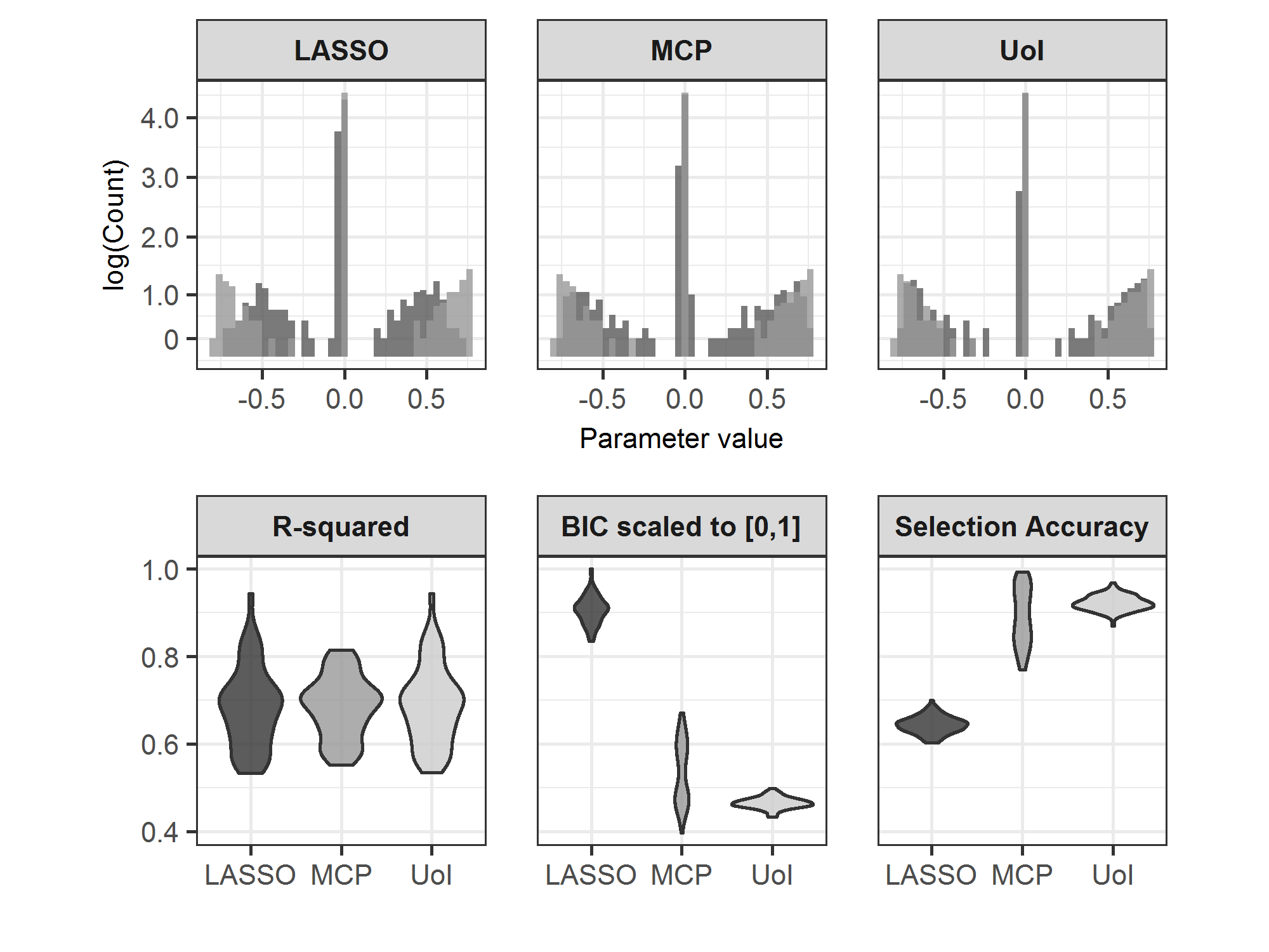
Figure 1: Results from simulation study. Top, histograms of average estimate across all simulations for each method (darker shade) superimposed on true parameter distribution (lighter shade); bottom, fit and selection accuracy for each method. $UoI_{VAR}$ demonstrates less bias on average and superior selection accuracy while maintaining comparable model fit. Thus the method yields simultaneously parsimonious and well-fitting models.

The secondary simulations shown in the Supplement compare the performance of $UoI_{VAR}$ with the benchmark method on smaller processes (process dimension $M=20$) under difficult-to-recover parameter configurations (nonzero process parameters drawn from uniform and Laplacian distributions centered at zero). Under these difficult parameter settings, $UoI_{VAR}$ performs no worse than the benchmark, and provides slight improvements in the sense that the method has lower sensitivity but higher specificity than the benchmark with respect to zero/nonzero parameter classification. Thus, $UoI_{VAR}$ appears to perform more reliable selection in difficult problems (i.e., with data exhibiting weak dependence), which is highly valuable in causal discovery applications where low specificity is crucial.

4.2 Data Analysis

$UoI_{VAR}$ was used to learn putative causal connections between weekly closes of 50 randomly chosen publicly traded companies listed on the S&P 500 index in 2013-2014. This dataset was chosen due to the absence of benchmark datasets with known ground truth for large multivariate time series; the years 2013-2014 saw a steadily climbing index with no major disturbances. To obtain an approximately stationary process, first-order differences were calculated from the raw series; then, $VAR(1)$ model parameters were estimated from these differences using $UoI_{VAR}$. Plots of the raw series and the first differences for these data are provided in the supplement.

In causal discovery contexts, model output is often visualized as a directed graph comprising nodes representing each vector component and edges indicating the set of nonzero parameters. This reflects the idea that temporal interdependence among component series arises from a connectivity structure or physical network among the underlying phenomena measured to obtain data, and conveys a sense of the complexity of potential causal connections by the density of the graph.

The $UoI_{VAR}$ estimate obtained from analysis of the S&P 500 data is extremely sparse, comprising only 44 nonzero transition matrix parameters of a potential 2500. The corresponding network visualization is shown in Figure 2. Hyperparameters were set at $B1=20$, $B2=10$, $s=1$, $L=12$, and $\alpha=1$, and the regularization path for $\lambda$ was chosen from a LASSO path that spanned the full model space. $44$ nonzero parameters were estimated, not including intercepts, resulting in $98.24\%$ sparsity. Predictive accuracy was assessed by computing one-step conditional forecasts for each timepoint after $t=3$ (since a first-order model was fit to first order differences) as $\hat{X}_{t}=\hat{A}X_{t-1}$ and estimating root mean square error ($RMSE$) of one-step forecasts as $\frac{1}{(T-3)}\sum_{t=3}^{T}(X_{t}-\hat{X}_{t})(X_{t}-\hat{X}_{t})^{T}$. Estimated $RMSE$ was 11.42 overall, yet forecast errors were highly variable by company, as per-company estimates ranged from 1.43 (Robert Half International) to 44.99 (Google) and the interquartile range of these estimates spanned 4.72 to 8.33. The overall average of raw forecast errors was -0.214.

The model estimated by $UoI_{VAR}$ represents fewer than 1.8% of all possible connections among 50 randomly chosen companies spanning multiple economic sectors listed on the S&P index, yet produces accurate forecasts for many of these companies based on endogenous influences alone at only one order of temporal dependence. Given that first-order endogenous influences on the weekly scale are unlikely to capture the complex economic influences thought to underlie the behavior of equity share prices, this constitutes strong predictive performance, and together with the sparsity of the model, that predictive performance is linked directly to a simple and interpretable structure.

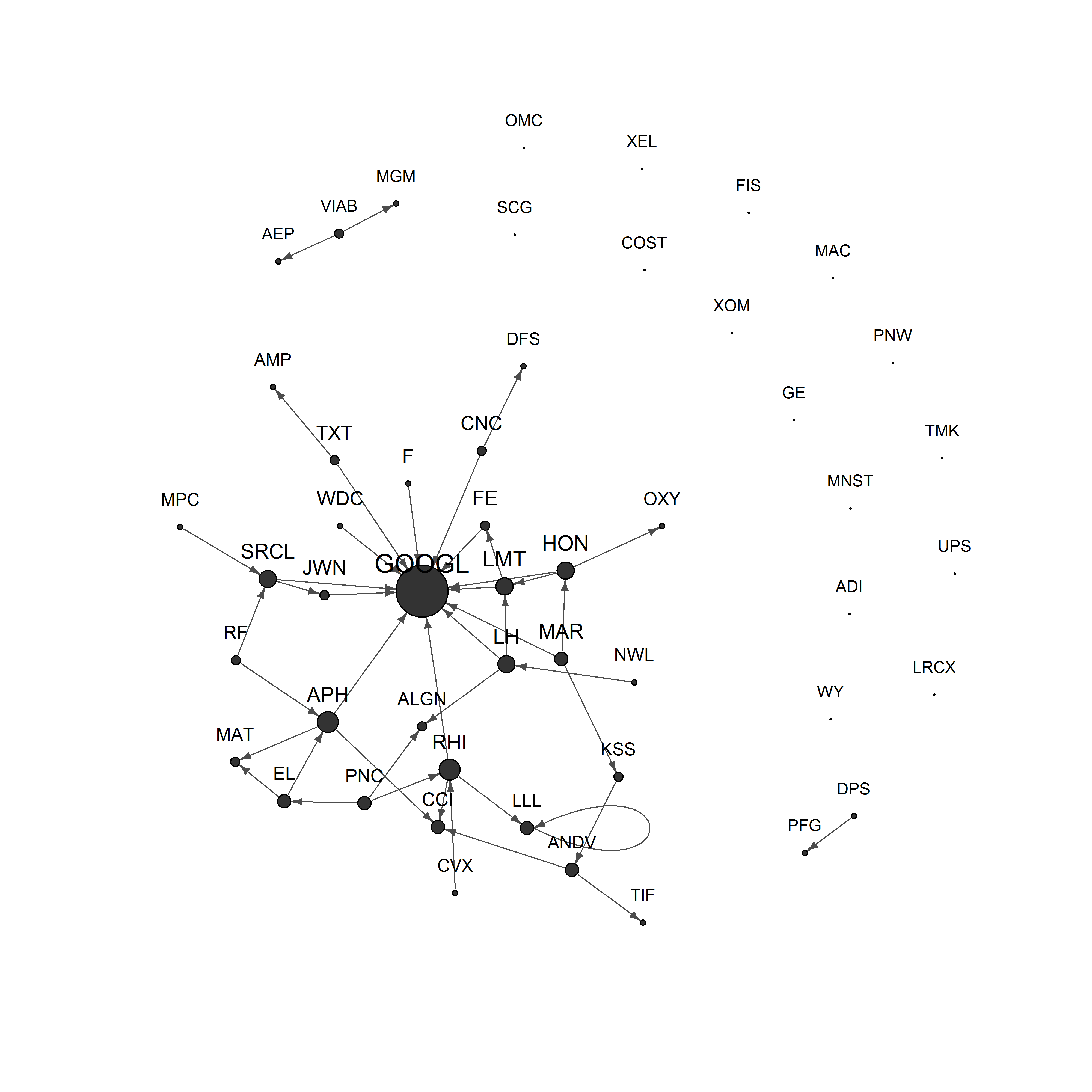
Figure 2: Network visualization of $UoI_{VAR}$ estimate of $VAR(1)$ model parameters for S&P 500 data. Node and label size are proportional to degree centrality. Google is central in terms of inward edges and connected to companies spanning a diverse range of sectors, but not outward edges, suggesting complex dependence of the company on other industry sectors yet little influence on other companies.

4.3 Algorithmic Scaling

The $UoI$ framework has innate algorithmic parallelism that can be exploited in scaling $UoI_{VAR}$ by bootstrap level parallelism and regularization path parallelism. These parallelisms were implemented for $UoI_{VAR}$ in C++ using Message Passing Interface (MPI) for inter-nodal communication and the program was executed on Cori Knight’s Landing supercomputer at Lawrence Berkeley National Laboratory.

For regularization path parallelism, the LASSO Alternating Direction Method of Multipliers (LASSO-ADMM) algorithm [9], which computes LASSO estimates in a distributed fashion, was employed for each bootstrap sample in the intersection step, and LASSO-ADMM with the regularization parameter set to $\lambda=0$ was employed to compute the ordinary least squares (OLS) estimates used in the Union step. For bootstrap level parallelism, it was found that generating data for bootstrap samples in both the Intersection and Union steps can be quite challenging because of immense inter-nodal communication; a data distribution strategy developed specifically for the $UoI$ algorithmic framework [5] was used to address this challenge.

An analysis of the runtime performance of the algorithm with this distribution strategy using synthetic datasets demonstrated that under weak scaling, which refers to increasing dataset size concurrently with the number of computation cores, the LASSO-ADMM computation runtime remains nearly constant but the bootstrap sample generation runtime increases exponentially. A second analysis demonstrated that under strong scaling, which refers to increasing the number of computation cores while maintaining a fixed dataset size, the LASSO-ADMM computation runtime decreases linearly but the bootstrap sample generation runtime increases exponentially. Scaling in these experiments was reported as a function of the regression problem size (i.e., in terms of memory required to store $\bm{Y}$ and $\bm{U}$ arising from time series data, rather than as a function of the memory required to store the input time series $\bm{X}$); problem sizes ranged between 128GB and 8TB in the weak scaling runtime analysis, and were fixed at 1TB for the strong scaling runtime analysis. These analyses demonstrated that above a certain dataset size, roughly 2TB, bootstrap sample generation becomes the execution time bottleneck of the program.

5 Discussion

This paper proposes a novel method for low-bias and sparse estimation of multivariate AR models, presents simulations that show its advantages over existing alternatives, exemplifies its application in data analysis, and describes its algorithmic scalability. The method is highly modular, and the hyperparameters $B_{1}$ and $B_{2}$ and $s$ jointly allow the analyst to control tolerances for false discovery and false omission without explicitly specifying any a priori assumptions about sparsity structure: increasing $B_{1}$ and $s$ creates pressure toward more sparse models, and increasing $B_{2}$ creates pressure toward added density of weak influences. Theoretical results show high accuracy in selecting strong signals.

$UoI_{VAR}$ is modular in the sense that it is possible to modify the penalty, bootstrap method, fit criteria, and even the model itself. While the exposition given in this paper focuses on Gaussian $VAR$ models, any likelihood estimator with a sparsity-inducing regularizer could be considered. Thus, the method has the flexibility to accommodate a wide range of changes as needed to suit issues that may arise in practice. Such modifications could provide the basis for further methodological research. In particular, a much wider class of models than $VAR(D)$ are used in practice with analogous aims, such as point processes models [44], and could be incorporated into the framework presented here with likely improvements in domain-specific applications.

Two challenges for the $UoI_{VAR}$ method are: (i) tuning is required to determine algorithm hyperparameters, and so far no default settings appear to be uniformly optimal across multiple contexts; and (ii) bootstrap samples can exhibit variability with respect to statistics of the original dataset, and thus the possibility of overfitting at least occasionally based on spurious correlations in a small number of bootstrap samples during the union step can sometimes be problematic.

In addition to addressing these challenges, promising extensions of this work include: (i) development of $UoI$ methods for multivariate point process models; (ii) theoretical analysis of stability selection methods for time series data; and (iii) application of $UoI_{VAR}$ to specific interpretable scientific datasets.

Supplement

Proofs of Lemma 1, Lemma 2, Theorem 3 and Corollary 4

Proof of Lemma 1

To prove that $\mathbf{S}$ satisfies RE, we first show that the random matrix $\mathbf{V}^{*}=(\mathbf{U}^{*})^{T}\mathbf{U}^{*}/N$ satisfies $RE(\gamma,\tau)$ with high probability, for some $\gamma>0$, $\tau>0$. Then we extend the result to $\mathbf{S}$. First note that a $VAR(D)$ model can be converted to a $VAR(1)$ model by redefining the transition matrix. One can redefine data generating process in equation 2 as

$$\tilde{X}_{t}=\tilde{A}_{1}\tilde{X}_{t-1}+\tilde{\epsilon}_{t}$$ (13)

where,

$$\tilde{X}_{t}=\left(\begin{array}[]{c}X_{t}\\ X_{t-1}\\ \vdots\\ X_{t-D+1}\\ \end{array}\right)_{DM\times 1}$$ (14)

$$\tilde{A}_{1}=\left(\begin{array}[]{c:c:c:c}A_{1}&\cdots&A_{D-1}&A_{D}\\ \text{I}_{M}&\cdots&\bm{0}&\bm{0}\\ \vdots&\ddots&\vdots&\vdots\\ \bm{0}&\cdots&\text{I}_{M}&\bm{0}\\ \end{array}\right)_{DM\times DM}$$ (15)

$$\tilde{X}_{t}=\left(\begin{array}[]{c}\epsilon_{t}\\ \epsilon_{t-1}\\ \vdots\\ \epsilon_{t-D+1}\\ \end{array}\right)$$ (16)

In particular, each row of $\mathbf{U}$ and similarly $\mathbf{U}^{*}$ is centered Gaussian with covariance $\Omega_{\tilde{X}}(0)$. From Proposition 2.3 and 2.4 of [7], we get that, for any $v\in\mathbb{R}^{DM}$, $||v||\leq 1$ and any $\eta>0$,

$$\mathbb{P}\left[|v^{T}(\mathbf{V}-\Omega_{\tilde{X}}(0))v|>\eta\frac{\Lambda_{max}(\Sigma)}{\mu_{min}(\mathcal{A})}\right]\\ \leq 2\exp[-cN\min\{\eta,\eta^{2}\}]$$

where, $N=T-D+1$. Now, for the bootstrap sample $\{\mathbf{X}^{*}_{t}\}_{t=0}^{T}$ and corresponding $\mathbf{V}^{*}=(\mathbf{U}^{*})^{T}\mathbf{U}^{*}/N$, the result modifies such that, for any $v\in\mathbb{R}^{DM}$, $||v||\leq 1$ and any $\eta>0$,

$$\mathbb{P}\left[|v^{T}(\mathbf{V}^{*}-\Omega_{\tilde{X}}(0))v|>\eta\frac{\Lambda_{max}(\Sigma)}{\mu_{min}(\mathcal{A})}\right]\\ \leq 2\exp[-cN_{*}\min\{\eta,\eta^{2}\}]$$

where, $N_{*}=L-D+1$. Now using the discretization argument as used in [7], we get that by setting $\omega=c_{4}\frac{\Lambda_{max}(\bm{\Sigma})/\mu_{min}(\mathcal{A})}{\Lambda_{min}(\bm{\Sigma})/\mu_{max}(\mathcal{A})}$ and $\eta=\omega^{-1}$, the form,

$$v^{T}\mathbf{V}^{*}v\geq\gamma||v||^{2}-\gamma/s_{1}||v||_{1}^{2},\ \ \ \mbox{for all }v\in\mathbb{R}^{DM}$$

with probability at least $1-2\exp[-cN_{*}\min\{\omega^{-2},1\}+2s_{1}\log(DM)]$. Now, setting $s_{1}=\lceil(c/4)N_{*}\min\{\omega^{-2},1\}\log(DM)\rceil$, we see that $\mathbf{V}^{*}\sim RE(\mu,\tau)$. Now, following the same line of arguments in Lemma B.1 in [7], we get $\mathbf{S}\sim RE(\mu,\tau)$.

Proof of Lemma 2

In order to prove deviation condition, we make use of the identity,

$$||\mathbf{r}-\mathbf{S}\bm{\beta}^{*}||_{\infty}=\max_{1\leq h\leq D;1\leq i,j\leq M}|e_{i}^{T}(\mathbf{U}_{(h)}^{T}\mathbf{E}/N)e_{j}|$$

for $\mathbf{U}_{(h)}=[X_{T-h}\ldots X_{D-h}]^{T}$. Now, using Proposition 2.4 from [7], the concentration inequality can be formed using $\eta=c_{0}\sqrt{\log(q)/N_{*}}$ for the bootstrap sample as the effective minimum stationary sample size for the bootstrap sample is $N_{*}=L-D+1$.

Proof of Theorem 3

Proof of Theorem 3, follows from the use of Lemma 1 and 2 properties for the bootstrap sample $\{\mathbf{X}^{*}_{t}\}_{t=0}^{T}$. The argument is same as in proof of Proposition 4.1 of [7].

Proof of Corollary 4

Proof of Corollary 4 follows directly from the results of Theorem 3 and the fact that the bootstrap samples are drawn iid. So, by the intersection step, if any one of the support set has no false positive, the intersection of the support sets also has no false positive.

Supplementary Figures

Here two sets of supplementary figures are provided: (i) figures summarizing small-scale simulations of potential failure modes as Figures 3 and 4, which results are referenced briefly in the main body of the paper in Section 3.1; and (ii) plots of the raw series and first differences of the S&P data analyzed in Section 3.2.

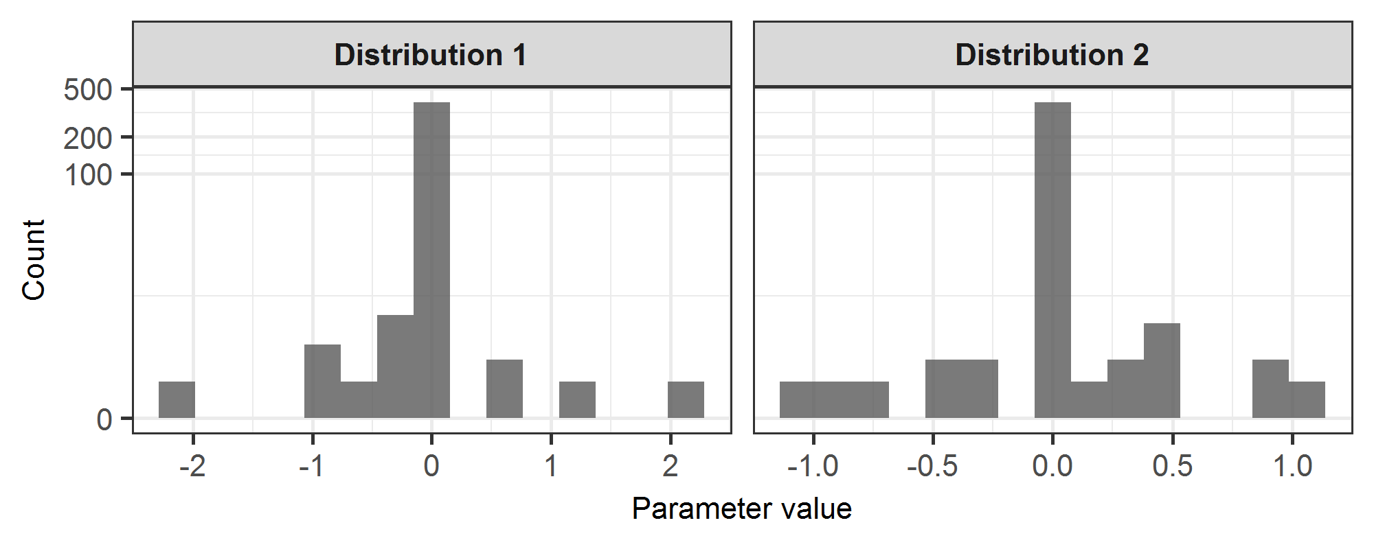
Figure 3: ‘Failure-mode’ distributions evaluated in a supplementary simulation. Left, nonzero coefficients drawn from a Laplacian distribution centered at 0; right, nonzero coefficients drawn from a uniform $[-1,1]$ distribution. Both are difficult to recover due to greater proportions of small-magnitude parameters.

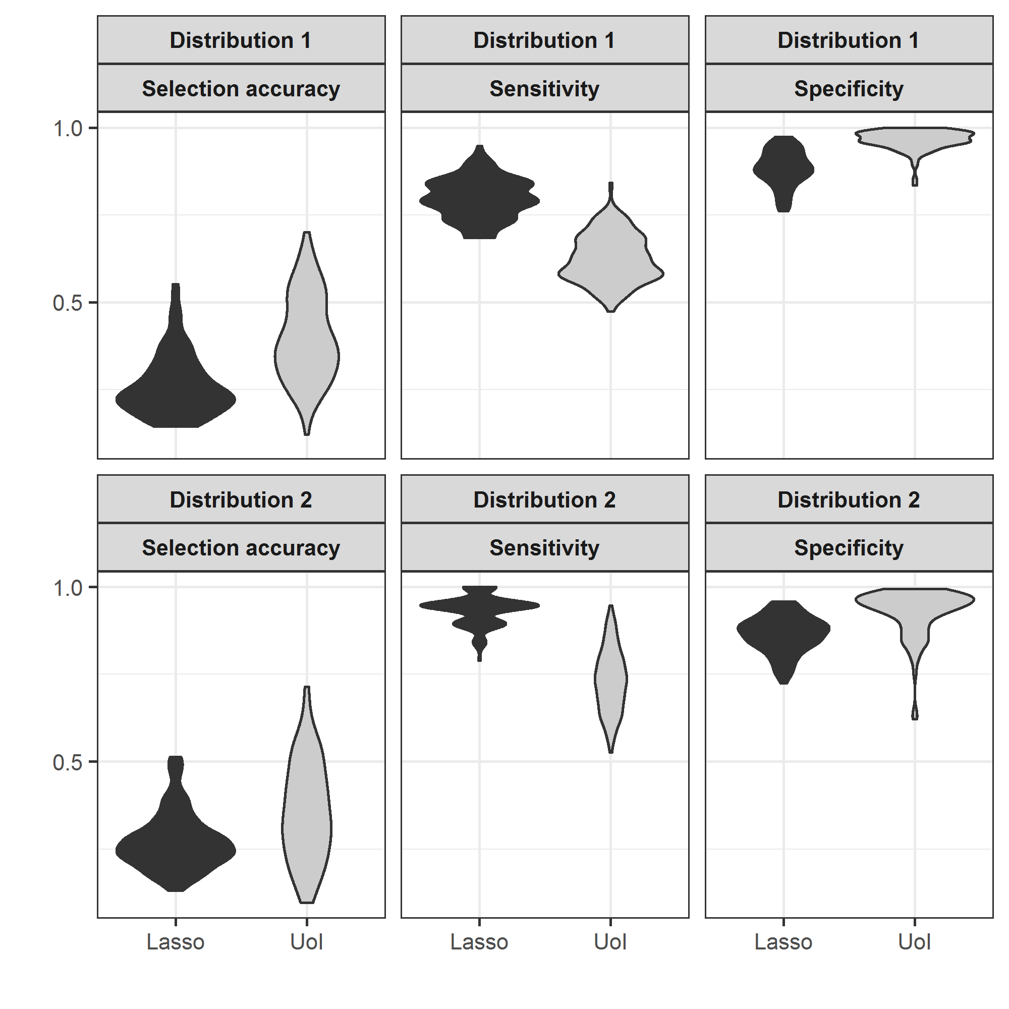
Figure 4: Results of simulation comparing LASSO and $UoI_{VAR}$ estimation on 100 simulated datasets from 20-dimensional $VAR(1)$ processes with coefficients from each failure-mode distribution. Overall neither method performs especially well, though $UoI_{VAR}$ exhibits greater specificity, reflecting less tendency toward overfitting and fewer false positives.

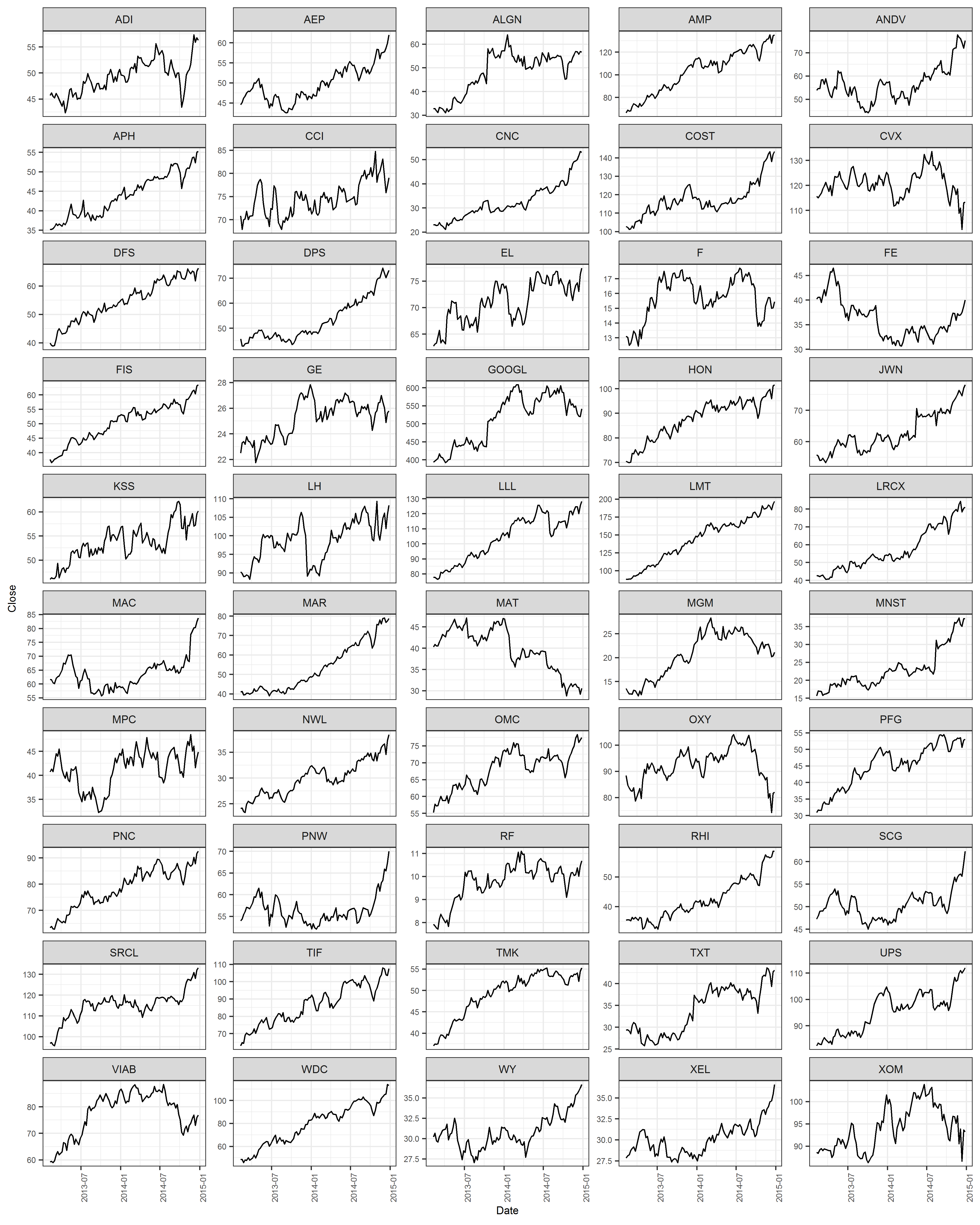
Figure 5: Plots of raw series of component time series of S&P data.

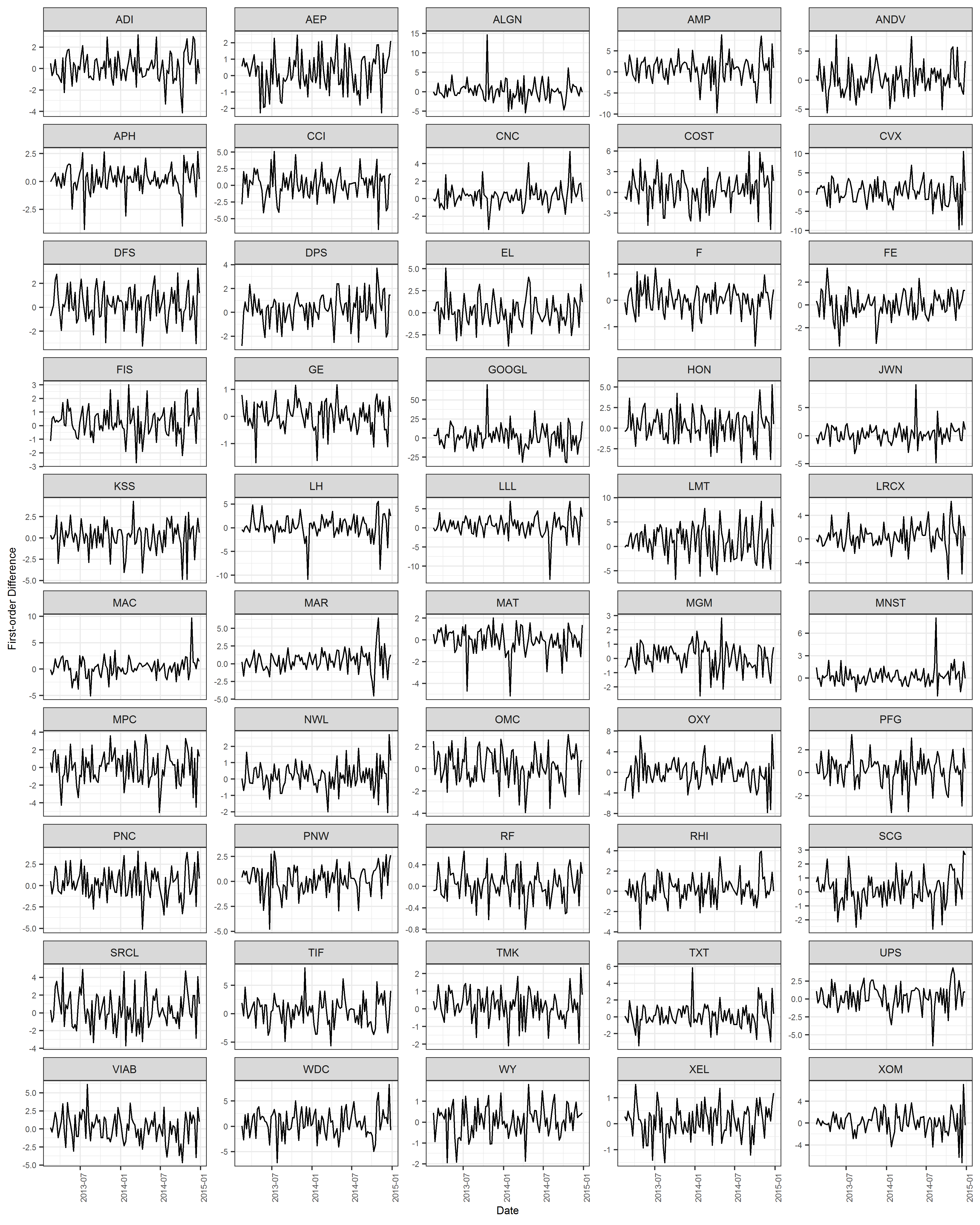
Figure 6: Plots of first differences of component time series of S&P data show that the first differences don’t obviously violate the stationarity assumption made in model fitting for the data analysis presented in the main paper.

References

- [1] Andrew Arnold, Yan Liu, and Naoki Abe. Temporal causal modeling with graphical granger methods. In Proceedings of the 13th ACM SIGKDD international confernce on knowledge discovery and data mining, pages 66–75. ACM, August 2007.
- [2] Laura Astolfi, Febo Cincotti, Donatella Mattia, M Grazia Marciani, Luiz A Baccala, Fabrizio de Vico Fallani, Serenella Salinari, Mauro Ursino, Melissa Zavaglia, Lei Ding, et al. Comparison of different cortical connectivity estimators for high-resolution eeg recordings. Human brain mapping, 28(2):143–157, 2007.
- [3] Francis Bach. Bolasso: model consistent lasso estimation through the boostrap. In Proceedings of the 25th International Conference on Machine Learning, pages 33–40. ACM, July 2008.
- [4] Francis Bach and Michael Jordan. Learning graphical models for stationary time series. IEEE Transactions on Signal Processing, 52(8):2189–2199, August 2004.
- [5] Mahesh Balasubramanian, Trevor Ruiz, Brandon Cook, Sharmodeep Bhattacharyya, Prabhat, Arival Shrivastava, and Kristofer Bouchard. Optimizing the union of intersections lasso and vector autoregressive algorithms for improved statistical estimation at scale. arXiv:1808.06992, 2018.
- [6] Danielle S Bassett, Nicholas F Wymbs, Mason A Porter, Peter J Mucha, Jean M Carlson, and Scott T Grafton. Dynamic reconfiguration of human brain networks during learning. Proceedings of the National Academy of Sciences, 108(18):7641–7646, 2011.
- [7] Sumanta Basu and George Michailidis. Regularized estimation in sparse high-dimensional time series models. The Annals of Statistics, 43(4):1535–1567, 2015.
- [8] Kristofer Bouchard, Alejandro Bujan, Farbod Roosta-Khorasani, Shashanka Ubaru, Mr Prabhat, Antoine Snijders, Jian-Hua Mao, Edward Chang, Michael W Mahoney, and Sharmodeep Bhattacharya. Union of intersections (uoi) for interpretable data driven discovery and prediction. In Advances in Neural Information Processing Systems, pages 1078–1086, 2017.
- [9] Stephen Boyd, Neal Parikh, Eric Chu, Borja Peleato, Jonathan Eckstein, et al. Distributed optimization and statistical learning via the alternating direction method of multipliers. Foundations and Trends® in Machine learning, 3(1):1–122, 2011.
- [10] Patrick Breheny and Jian Huang. Coordinate descent algorithms for nonconvex penalized regression, with applications to biological feature selection. The Annals of Applied Statistics, 5(1):232–253, 2011.
- [11] Leo Breiman. Bagging predictors. Machine Learning, 24:123–140, 1996.
- [12] Emery N Brown, Robert E Kass, and Partha P Mitra. Multiple neural spike train data analysis: state-of-the-art and future challenges. Nature neuroscience, 7(5):456–461, 2004.
- [13] Peter Bühlmann and Hans R Künsch. Block length selection in the bootstrap for time series. Computational Statistics & Data Analysis, 31(3):295–310, 1999.
- [14] Peter Bühlmann and Sara van de Geer. Statistics for High-Dimensional Data. Springer, 1 edition, 2011.
- [15] György Buzsáki, Costas Anastassiou, and Christof Koch. The origin of extracellular fields and currents – eeg, ecog, lfp and spikes. Nature Reviews Neuroscience, 13:407–420, June 2012.
- [16] Nik J Cunniffe, Britt Koskella, C Jessica E Metcalf, Stephen Parnell, Tim R Gottwald, and Christopher A Gilligan. Thirteen challenges in modelling plant diseases. Epidemics, 10:6–10, 2015.
- [17] Rainer Dahlhaus and Michael Eichler. Causality and graphical models in time series analysis. Oxford Statistical Science Series, pages 115–137, 2003.
- [18] Patrick Danaher, Pei Wang, and Daniela M Witten. The joint graphical lasso for inverse covariance estimation across multiple classes. Journal of the Royal Statistical Society: Series B (Statistical Methodology), 76(2):373–397, 2014.
- [19] Michael R DeWeese and Anthony M Zador. Non-gaussian membrane potential dynamics imply sparse, synchronous activity in auditory cortex. Journal of Neuroscience, 26(47):12206–12218, 2006.
- [20] James S Fackler and Sandra C Krieger. An application of vector time series techniques to macroeconomic forecasting. Journal of Business & Economic Statistics, 4(1):71–80, 1986.
- [21] Jianqing Fan, Jinchi Lv, and Lei Qi. Sparse high-dimensional models in economics. Annu. Rev. Econ., 3(1):291–317, 2011.
- [22] Mario Forni, Marc Hallin, Marco Lippi, and Lucrezia Reichlin. The generalized dynamic factor model: one-sided estimation and forecasting. Journal of the American Statistical Association, 100(471):830–840, 2005.
- [23] Jerome Friedman, Trevor Hastie, Holger Höfling, and Robert Tibshirani. Pathwise coordinate optimization. The Annals of Applied Statistics, 1(2):302–332, 2007.
- [24] Jerome Friedman, Trevor Hastie, and Robert Tibshirani. Regularization paths for generalized linear models via coordinate descent. Journal of Statistical Software, 33(1):1–22, 2010.
- [25] Clive Granger. Investigating causal relations by econometric models and cross-spectral methods. Econometrica, 37(3):424–438, 1969.
- [26] Jian Guo, Elizaveta Levina, George Michailidis, and Ji Zhu. Joint estimation of multiple graphical models. Biometrika, 98(1):1–15, 2011.
- [27] Eric C Hall, Garvesh Raskutti, and Rebecca Willett. Inferring high-dimensional poisson autoregressive models. In Statistical Signal Processing Workshop (SSP), 2016 IEEE, pages 1–5. IEEE, 2016.
- [28] Fang Han, Huanran Lu, and Han Liu. A direct estimation of high dimensional stationary vector autoregressions. Journal of Machine Learning Research, 16:3115–3150, 2015.
- [29] Anuj Karpatne, Imme Ebert-Uphoff, Sai Ravela, Hassan Ali Babaie, and Vipin Kumar. Machine learning for the geosciences: Challenges and opportunities. IEEE Transactions on Knowledge and Data Engineering, 2018.
- [30] Kendrick N Kay, Thomas Naselaris, Ryan J Prenger, and Jack L Gallant. Identifying natural images from human brain activity. Nature, 452(7185):352–355, 2008.
- [31] Jens-Peter Kreiss and Soumendra Nath Lahiri. Bootstrap methods for time series, volume 30 of Time Series Analysis: Methods and Applications, chapter 1, pages 3–26. Elsevier, 2012.
- [32] Hans R Kunsch et al. The jackknife and the bootstrap for general stationary observations. The Annals of Statistics, 17(3):1217–1241, 1989.
- [33] Regina Y Liu and Kesar Singh. Moving blocks jackknife and bootstrap capture weak dependence. Exploring the limits of bootstrap, 225:248, 1992.
- [34] Helmut Lütkepohl. New Introduction to Multiple Time Series Analysis. Springer, 1 edition, 2005.
- [35] Daniel A McFarland, Kevin Lewis, and Amir Goldberg. Sociology in the era of big data: The ascent of forensic social science. The American Sociologist, 47(1):12–35, 2016.
- [36] Nicolai Meinshausen and Peter Bühlmann. Stability selection. Journal of the Royal Statistical Society, 72(4):417–473, 2010.
- [37] Bijan Pesaran, Martin Vinck, Gaute Einevoll, Anton Sirota, Pascal Fries, Markus Siegel, Wilson Truccolo, Charles Schroeder, and Ramesh Srinivasan. Investigating large-scale brain dynamics using field potential recordings: analysis and interpretation. Nature neuroscience, 21(7):903–919, 2018.
- [38] Jonathan Pillow, Jonathon Shlens, Liam Paninski, Alexander Sher, Alan Litke, E. Chichilnisky, and Eero Simoncelli. Spatio-temporal correlations and visual signaling in a complete neuronal population. Nature, 454(7207):995–999, August 2008.
- [39] Huitong Qiu, Fang Han, Han Liu, and Brian Caffo. Joint estimation of multiple graphical models from high dimensional time series. Journal of the Royal Statistical Society: Series B (Statistical Methodology), 78(2):487–504, 2016.
- [40] Christopher A Sims. Macroeconomics and reality. Econometrica: Journal of the Econometric Society, pages 1–48, 1980.
- [41] Song Song and Peter J Bickel. Large vector auto regressions. arXiv preprint arXiv:1106.3915, 2011.
- [42] James H Stock and Mark W Watson. Forecasting using principal components from a large number of predictors. Journal of the American statistical association, 97(460):1167–1179, 2002.
- [43] Umberto Triacca, Alessandro Attanasio, and Antonello Pasini. Anthropogenic global warming hypothesis: testing its robustness by granger causality analysis. Environmetrics, 24(4):260–268, 2013.
- [44] Wilson Truccolo, Uri Eden, Matthew Fellows, John Donoghue, and Emery Brown. A point process framework for relating neural spiking activity to spiking history, neural ensemble, and extrinsic covariate effects. Journal of Neurophysiology, 93(2):1074–1089, February 2005.
- [45] Ruey S Tsay. Analysis of financial time series, volume 543. John Wiley & Sons, 2005.
- [46] Shashanka Ubaru, Kesheng Wu, and Kristofer E Bouchard. Uoi-nmfcluster: A robust nonnegative matrix factorization algorithm for improved parts-based decomposition and reconstruction of noisy data. In Machine Learning and Applications (ICMLA), 2017 16th IEEE International Conference on, pages 241–248. IEEE, 2017.
- [47] Hansheng Wang, Bo Li, and Chenlei Leng. Shrinkage tuning parameter selection with a diverging number of parameters. Journal of the Royal Statistical Society: Series B (Statistical Methodology), 71(3):671–683, 2009.
- [48] Tao Wang and Lixing Zhu. Consistent tuning parameter selection in high dimensional sparse linear regression. Journal of Multivariate Analysis, 102(7):1141–1151, 2011.
- [49] Cun-Hui Zhang. Nearly unbiased variable selection under minimax concave penalty. The Annals of Statistics, 38(2):894–942, 2010.