Potential Flow Generator with Optimal Transport Regularity for Generative Models
Abstract
We propose a potential flow generator with optimal transport regularity, which can be easily integrated into a wide range of generative models including different versions of GANs and flow-based models. We show the correctness and robustness of the potential flow generator in several 2D problems, and illustrate the concept of “proximity” due to the optimal transport regularity. Subsequently, we demonstrate the effectiveness of the potential flow generator in image translation tasks with unpaired training data from the MNIST dataset and the CelebA dataset.
1 Introduction
Many of the generative models, for example, generative adversarial networks (GANs) (Goodfellow et al., 2014; Arjovsky et al., 2017; Salimans et al., 2018) and flow-based models including normalizing flows (Rezende and Mohamed, 2015; Kingma and Dhariwal, 2018; Chen et al., 2018), aim to find a generator that could map the input distribution to the target distribution.
In many cases, especially when the input distribution is purely noises, the specific maps between input and output are of little importance as long as the generated distributions match the target ones. However, in other cases like image-to-image translations, where both input and target distributions are distributions of images, the generators are required to have additional regularity such that the input individuals are mapped to the “corresponding” outputs in some sense. If paired input-output samples are provided, penalty could be hybridized into generators loss functions to encourage the output individuals fit the ground truth (Isola et al., 2017). For the cases without paired data, a popular approach is to introduce another generator and encourage the two generators to be the inverse maps of each other, as in CycleGANs (Zhu et al., 2017), DualGANs (Yi et al., 2017) and DiscoGANs (Kim et al., 2017), etc. However, such a pair of generators is not unique and lacks clear mathematical interpretation about its effectiveness.
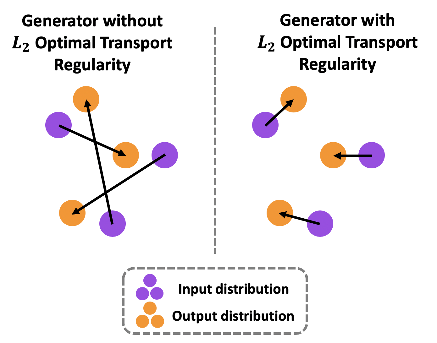
In this paper we introduce a special generator, i.e., the potential flow generator, with optimal transport regularity. It is not only a map from the input distribution to the target distribution, but also the optimal transport map with squared distance as transport cost. In Fig. 1 we provide a schematic comparison between generators with and without optimal transport regularity. Note that the generator with optimal transport regularity has the characteristic of “proximity”in that the inputs tend to be mapped to nearby outputs. As we will show later, this “proximity” characteristic of optimal transport regularity could be utilized in image translation tasks. Compared with other approaches like CycleGANs, the optimal transport regularity has a much clearer mathematical interpretation.
There have been other approaches to learn the optimal transport map in generative models. For example, Seguy et al. (2017) proposed to first learn the regularized optimal transport plan and then the optimal transport map, based on the dual form of regularized optimal transport problem. Also, Yang and Uhler (2018) proposed to learn the unbalanced optimal transport plan in an adversarial way derived from a convex conjugate representation of divergences. In the W2GAN model proposed by Leygonie et al. (2019), the discriminator’s objective is the 2-Wasserstein metric so that the generator is the optimal transport map. All the above approaches need to introduce, and are limited to, specific loss functions to train the generators. Our proposed potential flow generator takes a different approach in that with up to a slight augmentation of the original generator loss functions, our potential flow generator could be integrated into to a wide range of generative models with various generator loss functions, including different versions of GANs and flow-based models. This simple modification makes our method easy to adopt on various tasks considering the existing rich literature and the future developments of generative models.
Our main contributions are the following:
-
1.
We propose a potential flow generator with optimal transport regularity for a wide range of generative models. Two different versions are proposed: the discrete version and the continuous version.
-
2.
We compare the two versions and verify the correctness and robustness of the continuous potential flow generator by comparing it with analytical optimal transport maps. We also show the effectiveness of our methods in different generative models for more complicated distributions.
-
3.
We show the effectiveness of our generator with optimal transport regularity in image translation tasks with unpaired training data.
In Section 2 we give a formal definition of optimal transport map and the motivation to apply optimal transport regularity to generators. In Section 3 we give a detailed formulation of potential flow generator and the augmentation to the original loss functions. Results are then provided in Section 4. We include a discussion and conclusion in Section 5.
2 Generative Models and Optimal Transport Map
First, we introduce the concept of push forward, which will be used extensively in the paper.
Definition 1
Given two Polish space and , and the Borel -algebra on and , and the set of probability measures on and . Let be a Borel map, and . We define , the push forward of through , by
| (1) |
With the concept of push forward, we can formulate the goal of GANs and and flow-based models as to train the generator such that is equal to or at least close to in some sense, where and are the input and target distribution, respectively. Usually, the loss functions for training the generators are metrics of closeness that vary for different models. For example, in continuous normalizing flows (Chen et al., 2018), such metric of closeness is or . In Wasserstein GANs (WGANs) (Arjovsky et al., 2017), the metric of closeness is the Wasserstein-1 distance between and , which is estimated in a variational form with discriminator neural networks. As a result, the generator and discriminator neural networks are trained in an adversarial way:
| (2) |
where is the discriminator neural network and the Lipschitz constraint could be imposed via the gradient penalty (Gulrajani et al., 2017), spectral normalization (Miyato et al., 2018), etc.
Now we can introduce the concept of Monge’s optimal transport problem and the optimal transport map as following:
Definition 2
Given a cost function , and , , we let be the set of all transport maps from to , i.e. . Monge’s optimal transport problem is to minimize the cost functional among , where
| (3) |
and the minimizer is called the optimal transport map.
In this paper, we are concerned mostly about the case where with transport cost, i.e., the transport . Also, we assume that and are absolute continuous w.r.t. Lebesgue measure, i.e. they have probability density functions. Such problem is important for the following reasons:
-
1.
In general, Monge’s problem could be ill-posed in that could be empty set or there is no minimizer in . Moreover, the optimal transport map could be non-unique, for example, if transport cost . However, for the special case we consider, there exists a unique solution to Monge’s problem.
-
2.
Informally speaking, with transport cost the optimal transport map has the characteristic of “proximity”, i.e. the inputs tend to be mapped to nearby outputs. In image translation tasks, such “proximity” characteristic would be helpful if we could properly embed the images into Euclidean space such that our preferred input-output pairs are close to each other.
- 3.
3 Potential Flow Generator
3.1 Potential Flow Formulation of Optimal Transport Map
One of the most important results for the case we are studying is that the optimal map is of the form , where the so-called Brenier potential is convex and lower semi-continuous. We refer the readers to Gangbo and McCann (1996) and McCann and Guillen (2011) for the details. Note that the convexity constraint for is essential for optimality. Here is an example of non-convex leading to sub-optimal transport map: let and both be uniform distribution on , then the identical map which has zero cost is the optimal map, while we can construct a non-convex which leads to the sub-optimal transport map .
In the context of generative models, it looks plausible to represent the Brenier potential with a neural network and induce the generator from the gradient. However, the constraint of convexity is not trivial for neural networks. Therefore, we turned to another characterization of optimal transport map, i.e., the potential flow formulation which was firstly proposed by Benamou and Brenier (2000): suppose both and admit probability density and , and consider all smooth enough density field and velocity field , where , subject to the continuity equation as well as initial and final conditions
| (4) | ||||
The above equation actually says that such velocity field will induce a transport map: we can construct an ordinary differential equation (ODE)
| (5) |
and the map between initial point to final point gives the transport map from to .
As is proposed by Benamou and Brenier (2000), for the transport cost function , the minimal transport cost is equal to the infimum of
| (6) |
among all satisfying equation (4). The optimality condition is given by
| (7) | |||
In other words, the optimal velocity field is actually induced from a flow with time-dependent potential .
Note that different from the Brenier potential formulation, there is no explicit requirement for convexity in the potential flow formulation. This helps us to apply this formulation to design our generators with optimal transport regularity.
3.2 Potential Flow Generator
The potential is the key function to estimate, since the velocity field could be obtained by taking the gradient of the potential and consequently the transport map could be obtained from the ODE Eqn. 5. There are two strategies to use neural networks to represent .
-
1.
One can take advantage of the fact that the time-dependent potential field is actually uniquely determined by its initial condition from Eqn. 7, and use a neural network to represent the initial condition of , i.e. , while approximating via time discretization schemes.
-
2.
Alternatively, one can use a neural network to represent directly and later apply the PDE regularity for in Eqn. 7.
We name the generators defined in the above two approaches as discrete potential flow generator and continuous potential flow generator, respectively, and give a detailed formulation as follows.
3.2.1 Discrete Potential Flow Generator
In the discrete potential flow generator, we use the neural network with parameter to represent the initial condition of , i.e. . The potential field as well as the velocity field could then be approximated by different time discretization schemes, e.g. Eular schemes, Runge-Kutta schemes, etc. As an example, here we use the first-order forward Eular scheme for the simplicity of implementation. To be specific, suppose the time discretization step is and the number of total steps is with , then for , could be represented by , where
| (8) |
Consequently, the velocity field could be represented by , where
| (9) |
Finally, we can build the transport map from Eqs. 5:
| (10) | ||||
with be our transport map. The gradient w.r.t. in Eqns. 8, 9, 10 are realized by automatic differentiation.
The discrete potential flow generator has built-in optimal transport regularity since the optimal condition (Eqn. 7) is encoded in the time discretization (Eqn. 8). However, such discretization also introduces nested gradients, which dramatically increases computational cost when the number of total steps is increased. In our examples, we set and .
3.2.2 Continuous Potential Flow Generator
In the continuous potential flow generator, we use the neural network with parameters to represent . Consequently, we can represent the velocity field by , where
| (11) |
With the velocity field we could estimate the transport map by solving the ODE (Eqn. 5) using any numerical ODE solver. As an example, we can use the first-order forward Eular scheme, i.e.
| (12) | ||||
with be our transport map, where is the time discretization step and is the number of total steps with .
In the continuous potential flow generator, increasing the number of total steps would not introduce high order differentiations, therefore we could have very small time steps for a better precision of ODE solver. In practice, we set , in image translation tasks and elsewhere for continuous potential flow generators. Different from the discrete potential flow generator, the optimal condition (Eqn. 7) is not encoded in the continuous potential flow generator, therefore we need to penalize Eqn. 7 in the loss function, as we will discuss in the next subsection.
One may come up with another strategy of imposing the optimal transport regularity: to use a vanilla generator, which is a neural network directly mapping from inputs to outputs, and penalize the transport cost, i.e., the loss function is
| (13) |
where is the original loss function for the generator, and is the weight for the transport penalty. We emphasize that such strategy is much inferior to penalizing the PDE (Eqn. 7) in the continuous potential flow generator. When training the vanilla generator with transport penalty, no matter how we weight the transport cost penalty, in principle we always have to make a trade off between “matching the generated distribution with the target one” and “reducing the transport cost” since there is always a conflict between them, and consequently will be biased towards . On the other hand, there is no conflict between matching the distributions and penalizing Eqn. 7 in the continuous potential flow generator. As a consequence, the continuous potential flow generator is robust with respect to different weights for the PDE penalty. We will show this in Section 4.
3.3 Training the Potential Flow Generator
While the optimal condition (Eqn. 7) has been considered in the above two generators, the constraints of initial and final conditions are so far neglected. Actually, the constraint of initial and final conditions gives the principle to train the neural network: we need to tune the parameter in the neural network so that matches . This could be done by GANs or flow-based models.
3.3.1 Loss in GAN models
In the cases where the available data are samples from and , we could apply GAN models to train the potential flow generator. In particular, we replace the generator in GANs with the potential flow generator , feed samples from into , and view the outputs as “fake data” of . Both the discrete and continuous potential flow generator could be applied to such cases.
For the discrete potential flow generator, since the optimal transport regularity is already built in, the loss for training is simply the GAN loss for the generator, i.e.
| (14) |
where actually depends on the specific version of GANs. For example, if we use WGANs with gradient pernalty, then
| (15) |
where is the discriminator neural network.
For the continuous potential flow generator, as mentioned above, we also need to penalize the PDE (Eqn. 7) for the optimal transport regularity. Inspired by the applications of neural networks in solving forward and backward problems of PDEs, as in PINNs (Raissi et al., 2017a, b), we penalize the squared residual of the PDE on the so-called “residual" points. In particular, the loss for continuous potential flow generator would be
| (16) |
where are the residual points for the estimating the residual of PDE (Eqn. 7), and is the weight for the PDE penalty. While there could be other strategies to select the residual points, here we set them as the points on “trajectories” of input samples, i.e.
| (17) |
where is the set of batch samples from . Note that the coordinates of the residual points involves , but this should not be taken into consideration when calculating the gradient of loss function w.r.t. the generator parameters.
3.3.2 Loss in flow-based models
In the cases where we have density of distributions available, we could apply the continuous potential flow generator in flow-based models. Actually, our continuous potential flow generator perfectly matches the continuous normalizing flow model proposed by by Chen et al. (2018). Two ways are proposed to train the generator in continuous normalizing flow: density matching and maximum likelihood training. While both ways could be applied to train the continuous potential flow generators, here we take the latter one as an example, where we assume the density of and samples from are available, and we train the generator to maximize , where is the density of . Note that this is equivalent to minimizing . Consequently, the loss for the continuous potential flow generator would be:
| (18) |
where as in the GAN model, are the residual points for estimating the residual of PDE (Eqn. 7), and is the weight for the PDE penalty.
To estimate , we have the ODE that connects the probability density at inputs and outputs of the generator:
| (19) |
for all in the support of , where the initial probability density is the density of at input , while the terminal probability density is the density of at output . The expectation in the loss function is taken with ; we set and estimate by solving the ODE
| (20) |
with initial condition as and as the corresponding . Note that with the maximum likelihood training, the density of could be unnormalized, since multiplications with would merely lead to a constant difference in the loss function.
In practice, we also need to discretize Eqns. 19 and 20 properly when calculating . For example, we use the first-order Euler scheme with time step for total time interval . Note that the discrete potential flow cannot be trivially applied in flow-based models since we found that the time step size is too large to calculate the density accurately.
4 Results
In this section we show the numerical results of potential flow generators in different generative models. In specific, in Section 4.1 we show the results of potential flow generators applied on 2D problems and image translation tasks with GAN models, while in Section 4.2 we show the results in a flow-based model. The numerical experiments are based on Python package TensorFlow(Abadi et al., 2015).
4.1 Potential Flow Generator in GAN models
4.1.1 2D problems
In this subsection, we apply the potential flow generator to several two dimensional problems where samples from and are available.
We first study the following two problems where we know analytical solutions for the optimal transport maps.
-
1.
In the first problem we assume that both and are Gaussian distributions. Suppose , , then (Gelbrich, 1990) the minimum transport cost between and will be
(21) which is also known as the squared Wasserstein-2 distance between two Gaussian distributions. In particular, we consider the case
(22) In this case we can check that is the optimal transport map.
-
2.
In the second problem we assume that and are concentrated on concentric rings. In polar coordinates, suppose that is the distribution with radius uniformly distributed on , while angular uniformly distributed on , and suppose is the distribution with radius uniformly distributed on , while angular uniformly distributed on . In this case we can check that in polar coordinates is the optimal transport map.
In both cases, we have 40000 samples from each of and as our training data. Samples from and as well as the optimal transport map in both cases are illustrated in Fig. 2(a) and Fig. 3(a).
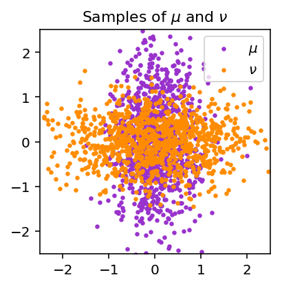
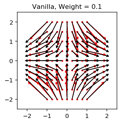
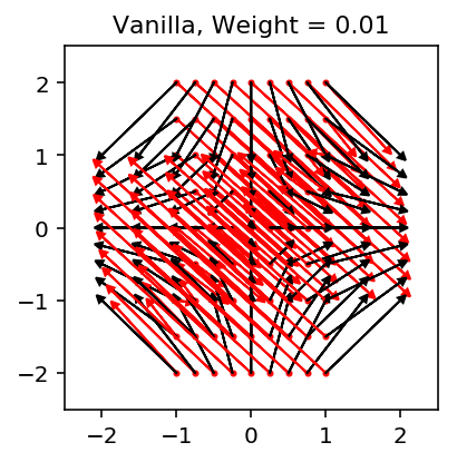
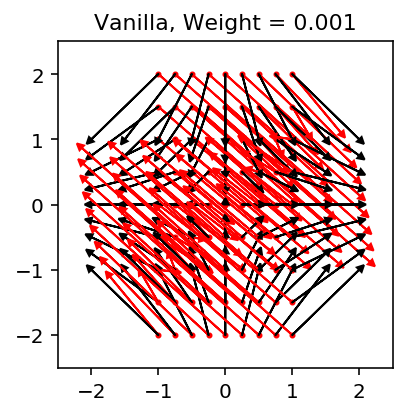
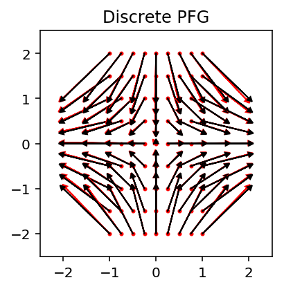
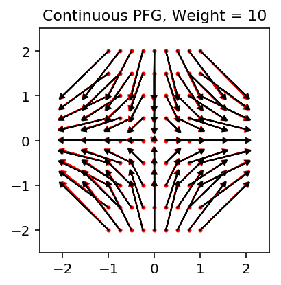
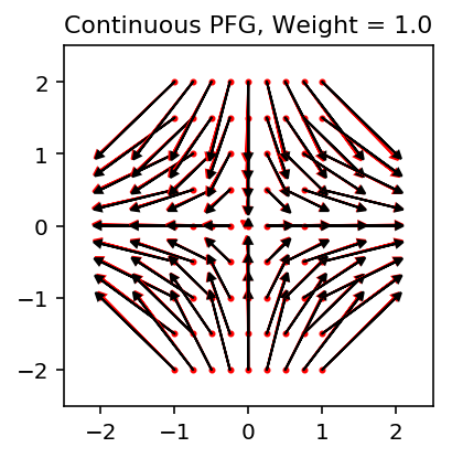
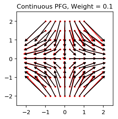
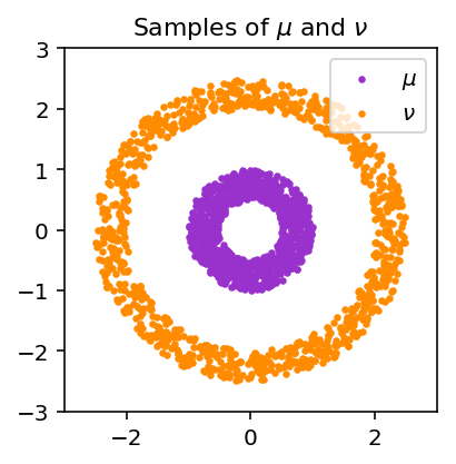
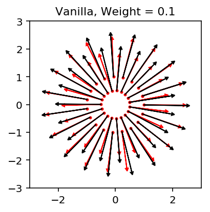
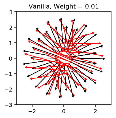
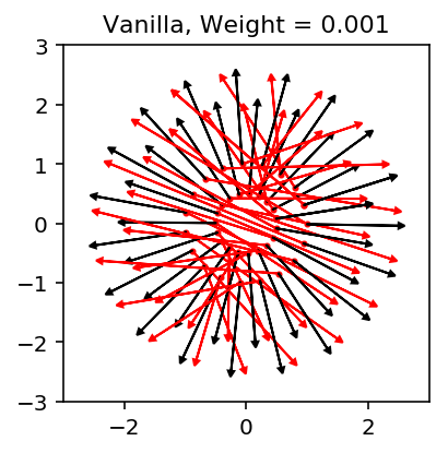
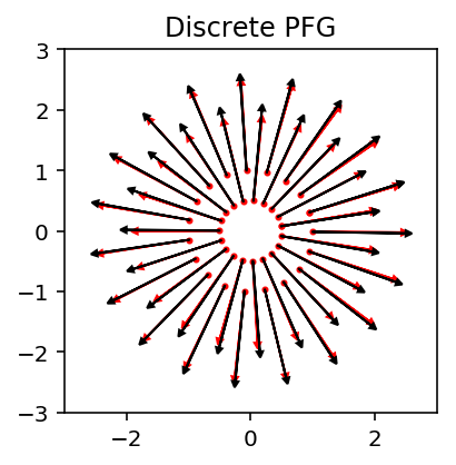
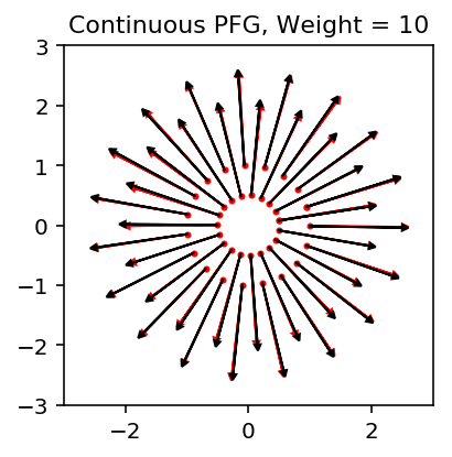
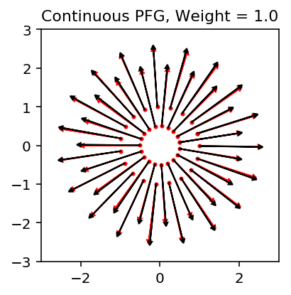
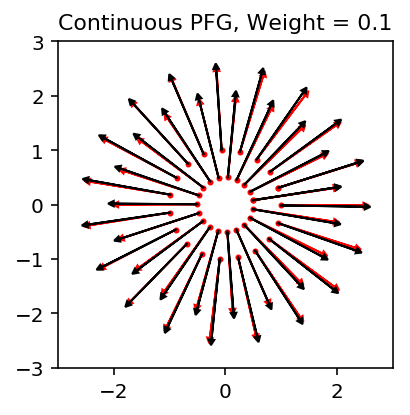
For the above two problems we compare the following generators: (a) vanilla generator, i.e., a neural network with a map from to that represents the transport map, with transport penalty added to the original loss function, i.e. loss function in Eqn. 13 with GAN loss as , (b) discrete potential flow generator, and (c) continuous potential flow generator with PDE penalty. For the vanilla generator and the continuous potential flow generator, we test different weights for the penalty in order to compare the influences of penalty weights in both methods. For all the generators the neural networks are designed as a feed forward neural network with 5 hidden layers, each of width 128, with a smooth function as the activation function since the velocity field has to be continuous. We use the Adam optimizer (Kingma and Ba, 2014) with learning rate , , , and train the neural networks for steps.
As for the GAN loss for generators we use the sliced Wasserstein distance111Strictly speaking, there is no “adversarial” training when we use sliced Wasserstein loss since the distance is estimated explicitly rather than represented by an other neural network. However, the idea of computing the distance between fake data and real data coincide with other GANs, especially WGANs. Therefore, in this paper we view sliced Wasserstein distance as a special version of GAN loss., due to its relatively low computational cost, robustness, and clear mathematical interpretation in low dimensional problems Deshpande et al. (2018). In particular, we estimate the sliced Wasserstein distances between samples of and using 1000 random projection directions. The batch size is set as 1000.
For all the cases we run the code three times using different random seed. In Fig. 2 we illustrate the transport maps in one of the three runs for each case. A more systematic and quantitative comparison is provided in Table 1 and Table 2, where the best results are marked as bold.
| Generator | Std in x-axis | Std in y-axis | Error of map |
|---|---|---|---|
| Reference | 1.000 | 0.500 | |
| Vanilla () | 0.9190.004 | 0.5920.003 | 0.1080.002 |
| Vanilla () | 0.9850.005 | 0.4990.006 | 0.4390.587 |
| Vanilla () | 0.9920.009 | 0.4930.001 | 0.4620.593 |
| Discrete PFG | 0.9930.001 | 0.4980.002 | 0.0180.006 |
| Continuous PFG () | 0.9910.001 | 0.5020.001 | 0.0180.006 |
| Continuous PFG () | 0.9920.001 | 0.4990.002 | 0.0190.007 |
| Continuous PFG () | 0.9900.002 | 0.5030.003 | 0.0250.008 |
| Generator | Mean of norm | Error of map |
|---|---|---|
| Reference | 2.250 | |
| Vanilla () | 2.1070.002 | 0.1460.003 |
| Vanilla () | 2.2270.004 | 0.9731.319 |
| Vanilla () | 2.2430.002 | 1.0001.311 |
| Continuous PFG () | 2.2430.001 | 0.0240.004 |
| Continuous PFG () | 2.2450.000 | 0.0290.002 |
| Continuous PFG () | 2.2450.001 | 0.0310.004 |
As we already mentioned, the transport penalty would make biased towards to reduce the transport cost from to . This is clearly shown in both problems where the penalty weight is . Actually, we observed more significant biases with larger penalty weights. For the cases with smaller penalty weights , in some of the runs, while are close to , the estimated transport maps are far from the optimal ones, which shows that the transport penalty cannot provide sufficient regularity if the penalty weight is too small. These numerical results are consistent with our earlier discussion about the intrinsic limitation of the transport penalty.
On the other hand, the potential flow generators give better matching between and , as well as smaller errors between the estimated transport maps and the analytical optimal transport maps. Notably, in both problems the continuous potential flow generators give good results with a wide range of PDE penalty weights ranging from to , which shows the superiority of PDE penalty in the continuous potential flow generators compared with the transport penalty in vanilla generators. We also report that while in the first problem the discrete potential flow generator achieves a comparable result with the continuous potential flow generators, in the second problem we encountered “NAN" problems during training the discrete potential flow generator in some of the runs. This indicates that the discrete potential flow generator is not as robust as the continuous one, which could be attributed to the high order differentiations in the discrete potential flow generators.
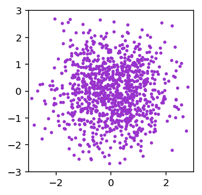
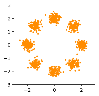
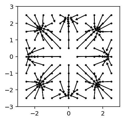
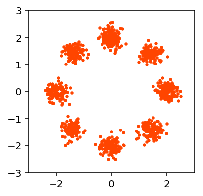
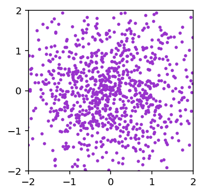
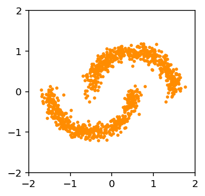
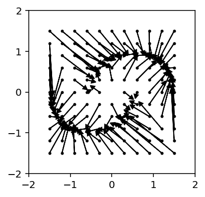
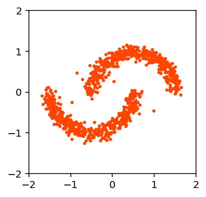
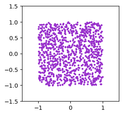
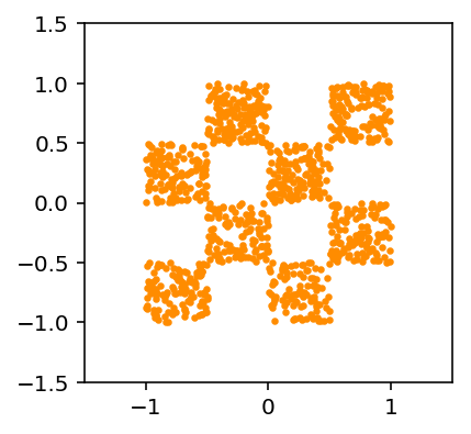
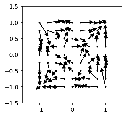
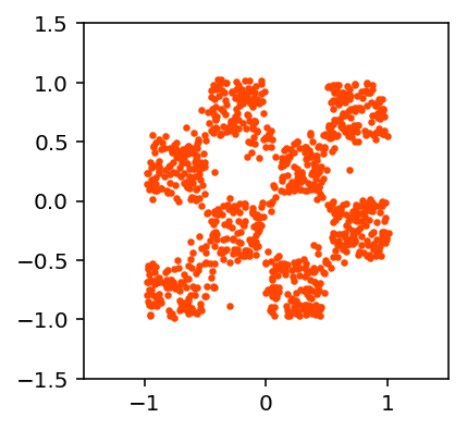
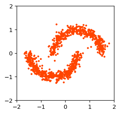
Apart from the previous two problems, we also applied the continuous potential flow generators to another three pairs of distributions, which are illustrated in Fig. 4. Here we use WGAN-GP instead of SWG since we found that it provides better GAN loss for complicated distributions. The PDE penalty weight are set as .
From Fig. 4 we can see the match between and in each of the problems, which shows the effectiveness of the potential flow generator. We could also see that samples of tend to be mapped to nearby positions, which demonstrates the characteristics of “proximity” in the potential flow generator maps due to the optimal transport regularity.
4.1.2 Image Translations: the MNIST and CelebA dataset
In this section, we aim to show the capability of potential flow generator in dealing with high dimensional problems, and also to show the potential of optimal transport map in tasks of image translations using unpaired training data. In particular, we apply the continuous potential flow generator, due to its robustness compared with the discrete potential flow generator, on the following two tasks:
-
1.
Translation between the MNIST images (LeCun et al., 2010). We divide the MNIST training dataset into two clusters: (a) images of digits 0 to 4, and (b) images of digits 5 to 9. We view the two clusters of images as samples of and , respectively, i.e., we want to find the optimal transport map from images of digits 0 to 4 to images of digits 5 to 9.
-
2.
Translation between the CelebA images (Liu et al., 2015). We randomly pick 60000 images from the CelebA training dataset and divide them into two clusters: (a) no-smiling face images, i.e., images with attribute “smiling” labeled as false, and (b) smiling face images, i.e., images with attribute “smiling” labeled as true. We crop the images so that only faces remain on the images, and view the two clusters as samples of and , respectively, i.e., we want to find to the optimal transport map from no-smiling face images to smiling face images.
Note that in both tasks there are no paired images in training data, and in the first task we do not distinguish digits among samples and samples.
Before feeding into the generators, we need to embed the images into a Euclidean space, where the distances between embedding vectors should quantify the similarities between images. While there could be other ways for the embedding, like auto-encoders or graph-embedding, in this paper we apply the principal component analysis (PCA)(Jolliffe, 2011), a simple but highly interpretable approach to conduct the image embedding. In both problems, we use WGAN-GP to provide the GAN loss functions. While keeping the time span , here we set the time step instead of to reduce the computational cost. The PDE penalty weight is set as 1.0. Both and the discriminator are designed as feed forward neural networks with 5 hidden layers, each of width 256. We emphasize that we did not use any convolutional neural networks here. We use the Adam optimizer with learning rate , , , and train the neural networks for steps.
For the first problem on the MNIST dataset, we embed the images into 100-dimensional Euclidean space, i.e. the total components in PCA is 100. We randomly pick images of digits from 0 to 4 from the test set and show the corresponding inputs and outputs in Fig. 5. Although the digits are mixed in the training dataset, we can see that after training, the potential flow generator tends to translate images of digit 0 to digit 6, digit 1 to digit 7, digit 3 to digit 5 or 8, and digit 4 to digit 9. This is consistent with our previous discussion about the characteristics of “proximity” in that the input digits and output digits “look similar”, and the corresponding embedding vectors should be close in the distance.


For the second problem on the CelebA dataset, we embed the images into a 700-dimensional Euclidean space, i.e. the total components in PCA is 700. We randomly pick no-smiling images from the training and testing datasets, and show the corresponding inputs and outputs in Fig. 6. We can see that for most of the images, the potential flow generator could translate the no-smiling faces to smiling faces while keeping the other attributes. We can also see the failure for other images, especially for side faces, which could be partially attributed to the fact that these images are outliers in PCA. The reconstructed output images are kind of blurred, since it is difficult to learn the high order modes of PCA.
4.2 Potential Flow Generator in flow-based models
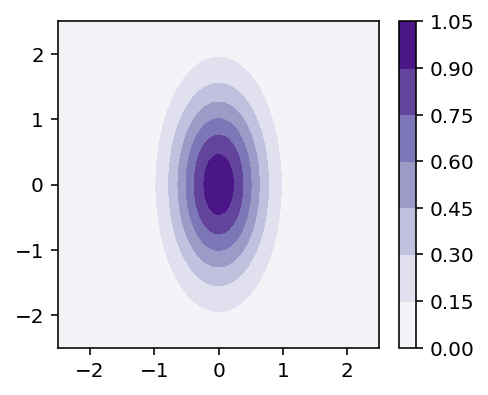
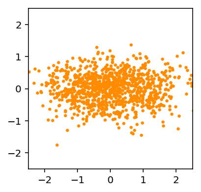
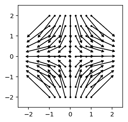
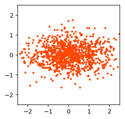
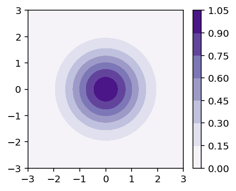
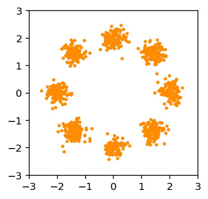
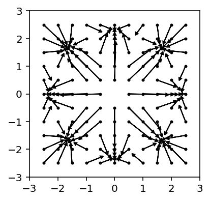
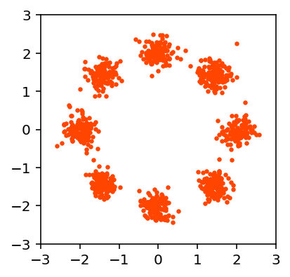
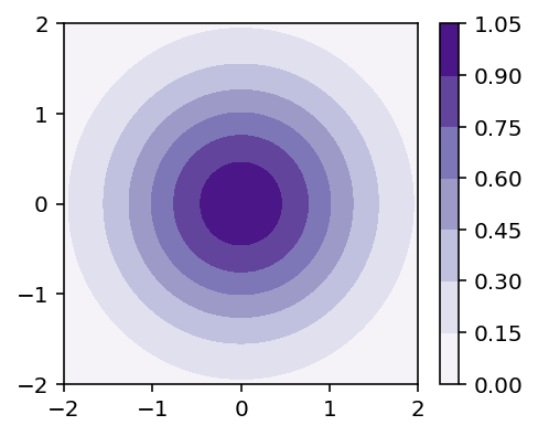
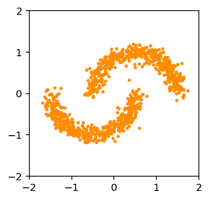
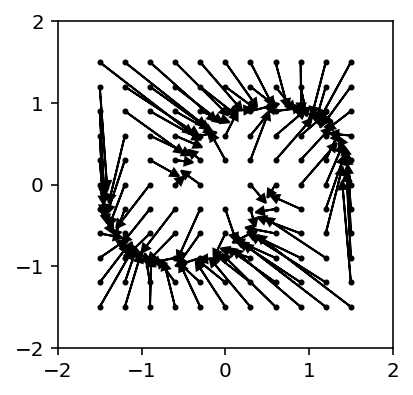
In this section we apply the continuous potential flow generator in continuous normalizing flows with three pairs of distributions. The distributions of and as well as the results are illustrated in Fig. 7. We use a feed forward neural network with 5 hidden layers, each of width 128, to represent . We use the Adam optimizer with learning rate , , , and train the neural networks for steps. The PDE penalty weights are set as . From Fig. 7 we can see the match between and in each of the problems, as well as that that the samples of tend to be mapped to nearby positions, which shows the effectiveness of the continuous potential flow generator in the flow-based models.
5 Conclusions
In this paper we propose potential flow generators with optimal transport regularity. In particular, we propose two versions: the discrete one and the continuous one. Both potential flow generators could be integrated in GAN models with various generator loss functions, while the latter one could also be integrated into flow-based models. For the discrete potential flow generator, the optimal transport is directly encoded in, while for the continuous potential flow generator we only need a slight augmentation to the original generator loss functions to impose the optimal transport regularity.
We first show the correctness of potential flow generators in estimating optimal transport map by comparing with analytical reference solutions. We report that the continuous potential flow generator outperforms the discrete one in robustness. We also illustrated the characteristic of “proximity” for potential flow generator due to optimal transport regularity, and consequently the effectiveness of the potential flow generator in image translation tasks using unpaired training data from the MNIST dataset and the CelebA dataset.
Apart from image-to-image translations, it is also possible to apply the potential flow generator to other translation tasks, text-to-text translations for example, if the translation objects could be properly embedded into Euclidean space. It is also interesting to study the application of potential flow generator in other generative models apart from the ones in this paper. Moreover, while in this paper we use PCA for image embedding, a possible improvement is to integrate potential flow generator with other embedding techniques like autoencoders and graph embedding methods. We leave these possible improvements to future work.
6 Acknowledgement
This work is supported by the ARO MURI project (W911NF-15-1-0562), the DOE PhILMs project (DE-SC0019453), and the DARPA AIRA project (HR00111990025).
References
- Abadi et al. (2015) Martín Abadi, Ashish Agarwal, Paul Barham, Eugene Brevdo, Zhifeng Chen, Craig Citro, Greg S. Corrado, Andy Davis, Jeffrey Dean, Matthieu Devin, Sanjay Ghemawat, Ian Goodfellow, Andrew Harp, Geoffrey Irving, Michael Isard, Yangqing Jia, Rafal Jozefowicz, Lukasz Kaiser, Manjunath Kudlur, Josh Levenberg, Dandelion Mané, Rajat Monga, Sherry Moore, Derek Murray, Chris Olah, Mike Schuster, Jonathon Shlens, Benoit Steiner, Ilya Sutskever, Kunal Talwar, Paul Tucker, Vincent Vanhoucke, Vijay Vasudevan, Fernanda Viégas, Oriol Vinyals, Pete Warden, Martin Wattenberg, Martin Wicke, Yuan Yu, and Xiaoqiang Zheng. TensorFlow: Large-scale machine learning on heterogeneous systems, 2015. URL https://www.tensorflow.org/. Software available from tensorflow.org.
- Ambrosio et al. (2008) Luigi Ambrosio, Nicola Gigli, and Giuseppe Savaré. Gradient flows: in metric spaces and in the space of probability measures. Springer Science & Business Media, 2008.
- Arjovsky et al. (2017) Martin Arjovsky, Soumith Chintala, and Léon Bottou. Wasserstein generative adversarial networks. In International Conference on Machine Learning, pages 214–223, 2017.
- Benamou and Brenier (2000) Jean-David Benamou and Yann Brenier. A computational fluid mechanics solution to the monge-kantorovich mass transfer problem. Numerische Mathematik, 84(3):375–393, 2000.
- Chen et al. (2018) Tian Qi Chen, Yulia Rubanova, Jesse Bettencourt, and David K Duvenaud. Neural ordinary differential equations. In Advances in Neural Information Processing Systems, pages 6571–6583, 2018.
- Deshpande et al. (2018) Ishan Deshpande, Ziyu Zhang, and Alexander G Schwing. Generative modeling using the sliced Wasserstein distance. In Proceedings of the IEEE Conference on Computer Vision and Pattern Recognition, pages 3483–3491, 2018.
- Gangbo and McCann (1996) Wilfrid Gangbo and Robert J McCann. The geometry of optimal transportation. Acta Mathematica, 177(2):113–161, 1996.
- Gelbrich (1990) Matthias Gelbrich. On a formula for the Wasserstein metric between measures on Euclidean and Hilbert spaces. Mathematische Nachrichten, 147(1):185–203, 1990.
- Goodfellow et al. (2014) Ian Goodfellow, Jean Pouget-Abadie, Mehdi Mirza, Bing Xu, David Warde-Farley, Sherjil Ozair, Aaron Courville, and Yoshua Bengio. Generative adversarial nets. In Advances in Neural Information Processing Systems, pages 2672–2680, 2014.
- Gulrajani et al. (2017) Ishaan Gulrajani, Faruk Ahmed, Martin Arjovsky, Vincent Dumoulin, and Aaron C Courville. Improved training of Wasserstein GANs. In Advances in Neural Information Processing Systems, pages 5767–5777, 2017.
- Isola et al. (2017) Phillip Isola, Jun-Yan Zhu, Tinghui Zhou, and Alexei A Efros. Image-to-image translation with conditional adversarial networks. In Proceedings of the IEEE Conference on Computer Vision and Pattern Recognition, pages 1125–1134, 2017.
- Jolliffe (2011) Ian Jolliffe. Principal component analysis. Springer, 2011.
- Kim et al. (2017) Taeksoo Kim, Moonsu Cha, Hyunsoo Kim, Jung Kwon Lee, and Jiwon Kim. Learning to discover cross-domain relations with generative adversarial networks. In Proceedings of the 34th International Conference on Machine Learning-Volume 70, pages 1857–1865. JMLR. org, 2017.
- Kingma and Ba (2014) Diederik P Kingma and Jimmy Ba. Adam: A method for stochastic optimization. arXiv preprint arXiv:1412.6980, 2014.
- Kingma and Dhariwal (2018) Durk P Kingma and Prafulla Dhariwal. Glow: Generative flow with invertible 1x1 convolutions. In Advances in Neural Information Processing Systems, pages 10215–10224, 2018.
- LeCun et al. (2010) Yann LeCun, Corinna Cortes, and CJ Burges. MNIST handwritten digit database. ATT Labs [Online]. Available: http://yann. lecun. com/exdb/mnist, 2, 2010.
- Leygonie et al. (2019) Jacob Leygonie, Jennifer She, Amjad Almahairi, Sai Rajeswar, and Aaron Courville. Adversarial computation of optimal transport maps. arXiv preprint arXiv:1906.09691, 2019.
- Liu et al. (2015) Ziwei Liu, Ping Luo, Xiaogang Wang, and Xiaoou Tang. Deep learning face attributes in the wild. In Proceedings of the IEEE International Conference on Computer Vision, pages 3730–3738, 2015.
- McCann and Guillen (2011) Robert J McCann and Nestor Guillen. Five lectures on optimal transportation: geometry, regularity and applications. Analysis and geometry of metric measure spaces: lecture notes of the séminaire de Mathématiques Supérieure (SMS) Montréal, pages 145–180, 2011.
- Miyato et al. (2018) Takeru Miyato, Toshiki Kataoka, Masanori Koyama, and Yuichi Yoshida. Spectral normalization for generative adversarial networks. arXiv preprint arXiv:1802.05957, 2018.
- Otto (1997) Felix Otto. Viscous fingering: an optimal bound on the growth rate of the mixing zone. SIAM Journal on Applied Mathematics, 57(4):982–990, 1997.
- Raissi et al. (2017a) Maziar Raissi, Paris Perdikaris, and George Em Karniadakis. Physics informed deep learning (part i): Data-driven solutions of nonlinear partial differential equations. arXiv preprint arXiv:1711.10561, 2017a.
- Raissi et al. (2017b) Maziar Raissi, Paris Perdikaris, and George Em Karniadakis. Physics informed deep learning (part ii): Data-driven discovery of nonlinear partial differential equations. arXiv preprint arXiv:1711.10566, 2017b.
- Rezende and Mohamed (2015) Danilo Jimenez Rezende and Shakir Mohamed. Variational inference with normalizing flows. arXiv preprint arXiv:1505.05770, 2015.
- Salimans et al. (2018) Tim Salimans, Han Zhang, Alec Radford, and Dimitris Metaxas. Improving GANs using optimal transport. arXiv preprint arXiv:1803.05573, 2018.
- Santambrogio (2017) Filippo Santambrogio. Euclidean, metric, and Wasserstein gradient flows: an overview. Bulletin of Mathematical Sciences, 7(1):87–154, 2017.
- Seguy et al. (2017) Vivien Seguy, Bharath Bhushan Damodaran, Rémi Flamary, Nicolas Courty, Antoine Rolet, and Mathieu Blondel. Large-scale optimal transport and mapping estimation. arXiv preprint arXiv:1711.02283, 2017.
- Yang and Uhler (2018) Karren D Yang and Caroline Uhler. Scalable unbalanced optimal transport using generative adversarial networks. arXiv preprint arXiv:1810.11447, 2018.
- Yi et al. (2017) Zili Yi, Hao Zhang, Ping Tan, and Minglun Gong. DualGAN: Unsupervised dual learning for image-to-image translation. In Proceedings of the IEEE International Conference on Computer Vision, pages 2849–2857, 2017.
- Zhu et al. (2017) Jun-Yan Zhu, Taesung Park, Phillip Isola, and Alexei A Efros. Unpaired image-to-image translation using cycle-consistent adversarial networks. In Proceedings of the IEEE International Conference on Computer Vision, pages 2223–2232, 2017.