Global Reasoning over Database Structures for Text-to-SQL Parsing

Abstract

State-of-the-art semantic parsers rely on auto-regressive decoding, emitting one symbol at a time. When tested against complex databases that are unobserved at training time (zero-shot), the parser often struggles to select the correct set of database constants in the new database, due to the local nature of decoding. In this work, we propose a semantic parser that globally reasons about the structure of the output query to make a more contextually-informed selection of database constants. We use message-passing through a graph neural network to softly select a subset of database constants for the output query, conditioned on the question. Moreover, we train a model to rank queries based on the global alignment of database constants to question words. We apply our techniques to the current state-of-the-art model for Spider, a zero-shot semantic parsing dataset with complex databases, increasing accuracy from 39.4% to 47.4%.

1 Introduction

The goal of zero-shot semantic parsing Krishnamurthy et al. (2017); Xu et al. (2017); Yu et al. (2018b, a); Herzig and Berant (2018) is to map language utterances into executable programs in a new environment, or database (DB). The key difficulty in this setup is that the parser must map new lexical items to DB constants that weren’t observed at training time.

Existing semantic parsers handle this mostly through a local similarity function between words and DB constants, which considers each word and DB constant in isolation. This function is combined with an auto-regressive decoder, where the decoder chooses the DB constant that is most similar to the words it is currently attending to. Thus, selecting DB constants is done one at a time rather than as a set, and informative global considerations are ignored.

Consider the example in Figure 1, where a question is mapped to a SQL query over a complex DB. After decoding SELECT, the decoder must now choose a DB constant. Assuming its attention is focused on the word ‘name’ (highlighted), and given local similarities only, the choice between the lexically-related DB constants (singer.name and song.name) is ambiguous. However, if we globally reason over the DB constants and question, we can combine additional cues. First, a subsequent word ‘nation’ is similar to the DB column country which belongs to the table singer, thus selecting the column singer.name from the same table is more likely. Second, the next appearance of the word ‘name’ is next to the phrase ’Hey’, which appears as the value in one of the cells of the column song.name. Assuming a one-to-one mapping between words and DB constants, again singer.name is preferred.

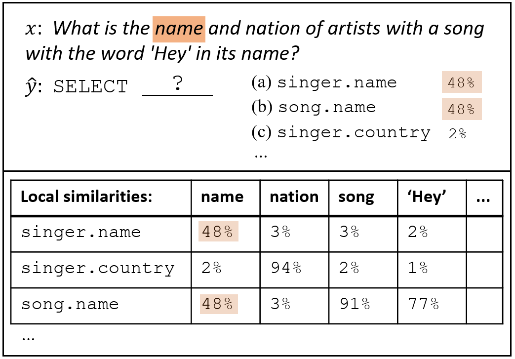
Figure 1: An example where choosing a DB constant based on local similarities is difficult, but the ambiguity can be resolved through global reasoning (see text).

In this paper, we propose a semantic parser that reasons over the DB structure and question to make a global decision about which DB constants should be used in a query. We extend the parser of Bogin et al. (2019), which learns a representation for the DB schema at parsing time. First, we perform message-passing through a graph neural network representation of the DB schema, to softly select the set of DB constants that are likely to appear in the output query. Second, we train a model that takes the top-$K$ queries output by the auto-regressive model and re-ranks them based on a global match between the DB and the question. Both of these technical contributions can be applied to any zero-shot semantic parser.

We test our parser on Spider, a zero-shot semantic parsing dataset with complex DBs. We show that both our contributions improve performance, leading to an accuracy of 47.4%, well beyond the current state-of-the-art of 39.4%.

Our code is available at https://github.com/benbogin/spider-schema-gnn-global.

2 Schema-augmented Semantic Parser

Problem Setup We are given a training set $\{(x^{(k)},y^{(k)},S^{(k)})\}_{k=1}^{N}$, where $x^{(k)}$ is a question, $y^{(k)}$ is its translation to a SQL query, and $S^{(k)}$ is the schema of the corresponding DB. We train a model to map question-schema pairs $(x,S)$ to the correct SQL query. Importantly, the schema $S$ was not seen at training time.

A DB schema $S$ includes : (a) A set of DB tables, (b) a set of columns for each table, and (c) a set of foreign key-primary key column pairs where each pair is a relation from a foreign-key in one table to a primary-key in another. Schema tables and columns are termed DB constants, denoted by $\mathcal{V}$.

We now describe a recent semantic parser from Bogin et al. (2019), focusing on the components relevant for selecting DB constants.

Base Model The base parser is a standard top-down semantic parser with grammar-based decoding Xiao et al. (2016); Yin and Neubig (2017); Krishnamurthy et al. (2017); Rabinovich et al. (2017); Lin et al. (2019). The input question $(x_{1},\dots,x_{|x|})$ is encoded with a BiLSTM, where the hidden states $\bm{e}_{i}$ of the BiLSTM are used as contextualized representations for the word $x_{i}$. The output query $y$ is decoded top-down with another LSTM using a SQL grammar, where at each time step a grammar rule is decoded. Our main focus is decoding of DB constants, and we will elaborate on this part.

The parser decodes a DB constant whenever the previous step decoded the non-terminals Table or Column. To select the DB constant, it first computes an attention distribution over the question words $\{\alpha_{i}\}_{i=1}^{|x|}$ in the standard manner Bahdanau et al. (2015). Then the score for a DB constant $v$ is $s_{v}=\sum_{i}\alpha_{i}s_{\text{link}}(v,x_{i})$, where $s_{\text{link}}$ is a local similarity score, computed from learned embeddings of the word and DB constant, and a few manually-crafted features, such as the edit distance between the two inputs and the fraction of string overlap between them. The output distribution of the decoder is simply $\text{softmax}(\{s_{v}\}_{v\in\mathcal{V}})$. Importantly, the dependence between decoding decisions for DB constants is weak – the similarity function is independent for each constant and question word, and decisions are far apart in the decoding sequence, especially in a top-down parser.

DB schema encoding In the zero-shot setting, the schema structure of a new DB can affect the output query. To capture DB structure, Bogin et al. (2019) learned a representation $\bm{h}_{v}$ for every DB constant, which the parser later used at decoding time. This was done by converting the DB schema into a graph, where nodes are DB constants, and edges connect tables and their columns, as well as primary and foreign keys (Figure 2, left). A graph convolutional network (GCN) then learned representations $\bm{h_{v}}$ for nodes end-to-end De Cao et al. (2019); Sorokin and Gurevych (2018).

To focus the GCN’s capacity on important nodes, a relevance probability $\rho_{v}$ was computed for every node, and used to “gate” the input to the GCN, conditioned on the question. Specifically, given a learned embedding $\bm{r}_{v}$ for every database constant, the GCN input is $\bm{h}^{(0)}_{v}=\rho_{v}\cdot\bm{r}_{v}$. Then, the GCN recurrence is applied for $L$ steps. At each step, nodes re-compute their representation based on the representation of their neighbors, where different edge types are associated with different learned parameters Li et al. (2016). The final representation of each DB constant is $\bm{h}_{v}=\bm{h}_{v}^{(L)}$.

Importantly, the relevance probability $\rho_{v}$, which can be viewed as a soft selection for whether the DB constant should appear in the output, was computed based on local information only: First, a distribution $p_{\text{link}}(v\mid x_{i})\propto\exp(s_{\text{link}}(v,x_{i}))$ was defined, and then $\rho_{v}=\max_{i}{p_{\text{link}}(v\mid x_{i})}$ was computed deterministically. Thus, $\rho_{v}$ doesn’t consider the full question or DB structure. We address this next.

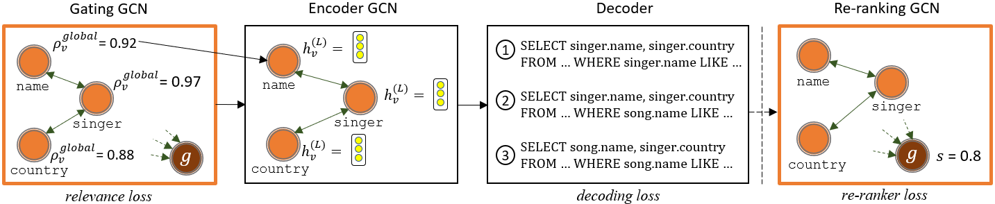
Figure 2: High-level overview, where our contributions are in thick orange boxes. First, a relevance score is predicted for each of the DB constants using the gating GCN. Then, a learned representation is computed for each DB constant using the encoder GCN, which is then used by the decoder to predict $K$ candidates queries. Finally, the re-ranking GCN scores each one of these candidates, basing its score only on the selected DB constants. The dashed line and arrow indicate no gradients are propagated from the re-ranking GCN to the decoder, as the decoder outputs SQL queries. Names of loss terms are written below models that are trained with a loss on their output.

3 Global Reasoning over DB Structures

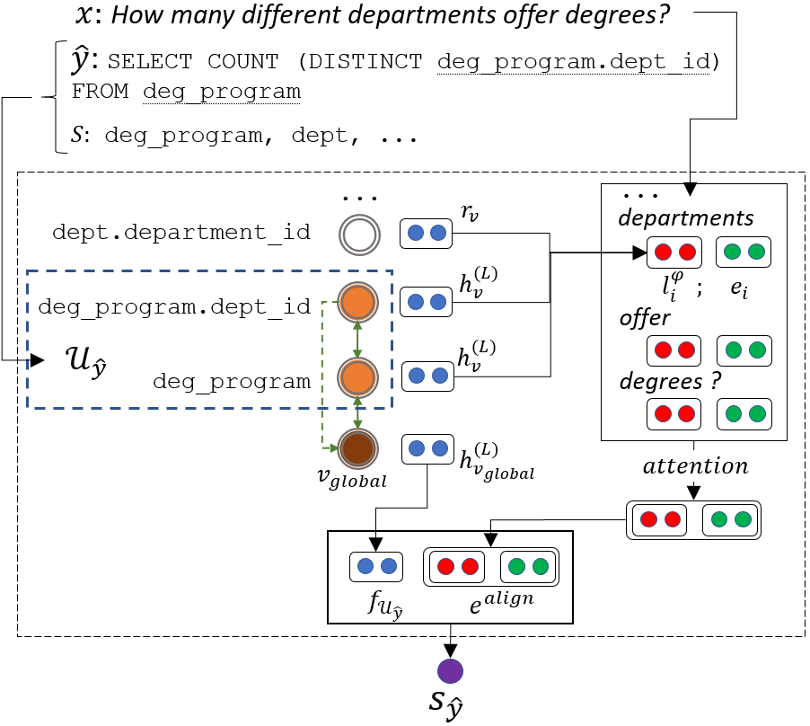
Figure 3: The re-ranking GCN architecture (see text).

Figure 2 gives a high-level view of our model, where the contributions of this paper are marked by thick orange boxes. First, the aforementioned relevance probabilities are estimated with a learned gating GCN, allowing global structure to be taken into account. Second, the model discriminatively re-ranks the top-$K$ queries output by the generative decoder.

Global gating Bogin et al. (2019) showed that an oracle relevance probability can increase model performance, but computed $\rho_{v}$ from local information only.

We propose to train a GCN to directly predict $\rho_{v}$ from the global context of the question and DB.

The input to the gating GCN is the same graph described in §2, except we add a new node $v_{\text{global}}$, connected to all other nodes with a special edge type. To predict the question-conditioned relevance of a node, we need a representation for both the DB constant and the question. Thus, we define the input to the GCN at node $v$ to be $\bm{g}^{(0)}_{v}=FF([\bm{r}_{v};\bar{\bm{h}}_{v};\rho_{v}])$, where ’;’ is concatenation, $FF(\cdot)$ is a feed-forward network, and $\bm{\bar{h}_{v}}=\sum_{i}p_{\text{link}}(x_{i}\mid v)\cdot\bm{e}_{i}$ is a weighted average of contextual representations of question tokens. The initial embedding of $v_{\text{global}}$ is randomly initialized. A relevance probability is computed per DB constant based on the final graph representation: $\rho_{v}^{\text{global}}=\sigma(FF(\bm{g}^{(L)}_{v}))$. This probability replaces $\rho_{v}$ at the input to the encoder GCN (Figure 2).

Because we have the gold query $y$ for each question, we can extract the gold subset of DB constants $\mathcal{U}_{y}$, i.e., all DB constants that appear in $y$. We can now add a relevance loss term $-\sum_{v\in\mathcal{U}_{y}}\log\rho_{v}^{\text{global}}-\sum_{v\notin\mathcal{U}_{y}}\log(1-\rho_{v}^{\text{global}})$ to the objective. Thus, the parameters of the gating GCN are trained from the relevance loss and the usual decoding loss, a ML objective over the gold sequence of decisions that output the query $y$.

Discriminative re-ranking Global gating provides a more accurate model for softly predicting the correct subset of DB constants. However, parsing is still auto-regressive and performed with a local similarity function. To overcome this, we separately train a discriminative model Collins and Koo (2005); Ge and Mooney (2006); Lu et al. (2008); Fried et al. (2017) to re-rank the top-$K$ queries in the decoder’s output beam. The re-ranker scores each candidate tuple $(x,S,\hat{y})$, and thus can globally reason over the entire candidate query $\hat{y}$.

We focus the re-ranker capacity on the main pain point of zero-shot parsing – the set of DB constants $\mathcal{U}_{\hat{y}}$ that appear in $\hat{y}$. At a high-level (Figure 3), for each candidate we compute a logit $s_{\hat{y}}=\bm{w}^{\top}FF(\bm{f}_{\mathcal{U}_{\hat{y}}},\bm{e}^{\text{align}})$, where $\bm{w}$ is a learned parameter vector, $\bm{f}_{\mathcal{U}_{\hat{y}}}$ is a representation for the set $\mathcal{U}_{\hat{y}}$, and $\bm{e}^{\text{align}}$ is a representation for the global alignment between question words and DB constants. The re-ranker is trained to minimize the re-ranker loss, the negative log probability of the correct query $y$. We now describe the computation of $\bm{f}_{\mathcal{U}_{\hat{y}}}$ and $\bm{e}^{\text{align}}$, based on a re-ranking GCN.

Unlike the gating GCN, the re-ranking GCN takes as input only the sub-graph induced by the selected DB constants $\mathcal{U}_{\hat{y}}$, and the global node $v_{\text{global}}$. The input is represented by $\bm{f}^{(0)}_{v}=FF(\bm{r}_{v};\bar{\bm{h}}_{v})$, and after L propagation steps we obtain $\bm{f}_{\mathcal{U}_{\hat{y}}}=\bm{f}^{(L)_{v_{\text{global}}}}$. Note that the global node representation is used to describe and score the question-conditioned sub-graph, unlike the gating GCN where the global node mostly created shorter paths between other graph nodes.

The representation $\bm{f}_{\mathcal{U}_{\hat{y}}}$ captures global properties of selected nodes but ignores nodes that were not selected and are possibly relevant. Thus, we compute a representation $\bm{e}^{\text{align}}$, which captures whether question words are aligned to selected DB constants. We define a representation for every node $v\in\mathcal{V}$:

$$\bm{\varphi}_{v}=\begin{cases}\bm{f}_{v}^{(L)}&\text{ if }v\in\mathcal{U}_{\hat{y}}\\ \bm{r}_{v}&\text{otherwise}\end{cases}$$

Now, we compute for every question word $x_{i}$ a representation of the DB constants it aligns to: $\bm{l}^{\varphi}_{i}=\sum_{v\in\mathcal{V}}p_{\text{link}}(v\mid x_{i})\cdot\bm{\varphi}_{v}$. We concatenate this representation to every word $\bm{e}_{i}^{\text{align}}=[\bm{e}_{i};\bm{l}^{\varphi}_{i}]$, and compute the vector $\bm{e}^{\text{align}}$ using attention over the question words, where the attention score for every word is $\bm{e}_{i}^{\text{align}\top}\bm{w}_{\text{att}}$ for a learned vector $\bm{w}_{\text{att}}$. The goal of this term is to allow the model to recognize whether there are any attended words that are aligned with DB constants, but these DB constants were not selected in $\mathcal{U}_{\hat{y}}$.

In sum, our model adds a gating GCN trained to softly select relevant nodes for the encoder, and a re-ranking GCN that globally reasons over the subset of selected DB constants, and captures whether the query properly covers question words.

4 Experiments and Results

Model	Accuracy
SyntaxSQLNet	19.7%
GNN	39.4%
Global-GNN	47.4%

Table 1: Test set accuracy of Global-GNN compared to prior work on Spider.

Model	Acc.	Beam	Single	Multi
SyntaxSQLNet	18.9%		23.1%	7.0%
GNN	40.7%		52.2%	26.8%
+ Re-implementation	44.1%	62.2%	58.3%	27.6%
Global-GNN	52.1%	65.9 %	61.6%	40.3%
- No Global Gating	48.8%	62.2%	60.9%	33.8%
- No Re-ranking	48.3%	65.9%	58.1%	36.8%
- No Relevance Loss	50.1%	64.8%	60.9%	36.6%
No Align Rep.	50.8%	65.9%	60.7%	38.3%
Query Re-ranker	47.8%	65.9%	55.3%	38.3%
Oracle Relevance	56.4%	73.5%

Table 2: Development set accuracy for various experiments. The column ‘Beam’ indicates the fraction of examples where the gold query is in the beam ($K=10$).

Experimental setup We train and evaluate on Spider Yu et al. (2018b), which contains 7,000/1,034/2,147 train/development/test examples, using the same pre-processing as Bogin et al. (2019). To train the re-ranker, we take $K=40$ candidates from the beam output of the decoder. At each training step, if the gold query is in the beam, we calculate the loss on the gold query and 10 randomly selected negative candidates. At test time, we re-rank the best $K=10$ candidates in the beam, and break re-ranking ties using the auto-regressive decoder scores (ties happen since the re-ranker considers the DB constants only and not the entire query). We use the official Spider script for evaluation, which tests for loose exact match of queries.

Results As shown in Table 1, the accuracy of our proposed model (Global-GNN) on the hidden test set is 47.4%, 8% higher than current state-of-the art of 39.4%. Table 2 shows accuracy results on the development set for different experiments. We perform minor modifications to the implementation of Bogin et al. (2019), improving the accuracy from 40.7% to 44.1% (details in appendix A). We follow Bogin et al. (2019), measuring accuracy on easier examples where queries use a single table (Single) and those using more than one table (Multi).

Global-GNN obtains 52.1% accuracy on the development set, substantially higher than all previous scores. Importantly, the performance increase comes mostly from queries that require more than one table, which are usually more complex.

Removing any of our two main contributions (No Global Gating, No Re-ranking) leads to a 4% drop in performance. Training without the relevance loss (No Relevance Loss) results in a 2% accuracy degrade. Omitting the representation $e^{\text{align}}$ from the re-ranker (No Align Rep.) reduces performance, showing the importance of identifying unaligned question words.

We also consider a model that ranks the entire query and not only the set of DB constants. We re-define $s_{\hat{y}}=\bm{w}^{\top}FF(\bm{f}_{\mathcal{U}_{\hat{y}}},\bm{h}^{\text{align}},\bm{h}^{\text{query}})$, where $\bm{h}^{\text{query}}$ is a concatenation of the last and first hidden states of a BiLSTM run over the output SQL query (Query Re-ranker). We see performance is lower, and most introduced errors are minor mistakes such as min instead of max. This shows that our re-ranker excels at choosing DB constants, while the decoder is better at determining the SQL query structure and the SQL logical constants.

Finally, we compute two oracle scores to estimate future headroom. Assuming a perfect global gating, which gives probability $1.0$ iff the DB constant is in the gold query, increases accuracy to 63.2%. Adding to that a perfect re-ranker leads to an accuracy of 73.5%.

Qualitative analysis Analyzing the development set, we find two main re-occurring patterns, where the baseline model is wrong, but our parser is correct. (a) coverage: when relevant question words are not covered by the query, which results in a missing joining of tables or selection of columns (b) precision: when unrelated tables are joined to the query due to high lexical similarity. Selected examples are in Appendix B.

Error analysis In 44.4% of errors where the correct query was in the beam, the selection of $\mathcal{U}$ was correct but the query was wrong. Most of these errors are caused by minor local errors, e.g., min/max errors, while the rest are due to larger structural mistakes, indicating that a global model that jointly selects both DB constants and SQL tokens might further improve performance. Other types of errors include missing or extra columns and tables, especially in complex queries.

5 Conclusion

In this paper, we demonstrate the importance of global decision-making for zero-shot semantic parsing, where selecting the relevant set of DB constants is challenging. We present two main technical contributions. First, we use a gating GCN that globally attends the input question and the entire DB schema to softly-select the relevant DB constants. Second, we re-rank the output of a generative semantic parser by globally scoring the set of selected DB-constants. Importantly, these contributions can be applied to any zero-shot semantic parser with minimal modifications. Empirically, we observe a substantial improvement over the state-of-the-art on the Spider dataset, showing the effectiveness of both contributions.

Appendix A Re-implementation

We perform a simple modification to Bogin et al. (2019). We add cell values to the graph, in a similar fashion to Krishnamurthy et al. (2017). Specifically, we extract the cells of the first 5000 rows of all tables in the schema, during the pre-processing phase. We then consider every cell $q$ of a column $c$, which has a partial match with any of the question words $(x_{1},\dots,x_{|x|})$. We then add nodes representing these cells to all of the model’s graphs, with extra edges $(c,q)$ and $(q,c)$.

Appendix B Selected examples

Selected examples are given in Table 3.

Category	Question	Schema	Predicted Queries
Coverage	Show the name of the teacher for the math course.	course: course_id, staring_date, course teacher: teacher_id, name, age, hometown course_arrange: course_id, teacher_id, grade	Baseline: SELECT teacher.name FROM teacher WHERE teacher.name = ’math’ Our Model: SELECT teacher.name FROM teacher JOIN course_arrange ON teacher.teacher_id = course_arrange.teacher_id JOIN course ON course_arrange.course_id = course.course_id WHERE course.course = ’math’
Coverage	Who is the first student to register? List the first name, middle name and last name.	students: student_id, current_address_id, first_name, middle_name, last_name, … student_enrolment: student_enrolment_id, degree_program_id, … …	Baseline: SELECT students.first_name, students.middle_name, students.last_name FROM students Our Model: SELECT students.first_name, students.middle_name, students.last_name FROM students ORDER BY students.date_first_registered LIMIT 1
Coverage	List all singer names in concerts in year 2014.	singer: singer_id, name, country, song_name, song_release_year, … concert: concert_id, concert_name, year, … singer_in_concert: concert_id, singer_id …	Baseline: SELECT singer.name FROM singer WHERE singer.song_release_year = 2014 Our Model: SELECT singer.name FROM singer JOIN singer_in_concert ON singer.singer_id = singer_in_concert.singer_id JOIN concert ON singer_in_concert.concert_id = concert.concert_id WHERE concert.year = 2014
Precision	What are the makers and models?	car_makers: id, maker, fullname, country model_list: modelid, maker, model …	Baseline: SELECT car_makers.maker, model_list.model FROM car_makers JOIN model_list ON car_makers.id = model_list.maker Our Model: SELECT model_list.maker, model_list.model FROM model_list
Precision	Return the id of the document with the fewest paragraphs.	documents: document_id, document_name, document_description, … paragraphs: paragraph_id, document_id, paragraph_text, … …	Baseline: SELECT documents.document_id FROM documents JOIN paragraphs ON documents.document_id = paragraphs.document_id GROUP BY documents.document_id ORDER BY COUNT(*) LIMIT 1 Our Model: SELECT paragraphs.document_id FROM paragraphs GROUP BY paragraphs.document_id ORDER BY COUNT(*) ASC LIMIT 1

Table 3: Selected correct examples where the baseline model is wrong, but our parser is correct.

References

- Bahdanau et al. (2015) D. Bahdanau, K. Cho, and Y. Bengio. 2015. Neural machine translation by jointly learning to align and translate. In International Conference on Learning Representations (ICLR).
- Bogin et al. (2019) B. Bogin, M. Gardner, and J. Berant. 2019. Representing schema structure with graph neural networks for text-to-sql parsing. In Association for Computational Linguistics (ACL).
- Collins and Koo (2005) M. Collins and T. Koo. 2005. Discriminative reranking for natural language parsing. Computational Linguistics, 31(1):25–70.
- De Cao et al. (2019) N. De Cao, W. Aziz, and I. Titov. 2019. Question answering by reasoning across documents with graph convolutional networks. In North American Association for Computational Linguistics (NAACL).
- Fried et al. (2017) D. Fried, M. Stern, and D. Klein. 2017. Improving neural parsing by disentangling model combination and reranking effects. In Association for Computational Linguistics (ACL).
- Ge and Mooney (2006) R. Ge and R. J. Mooney. 2006. Discriminative reranking for semantic parsing. In Proceedings of the COLING/ACL 2006 Main Conference Poster Sessions, pages 263–270.
- Herzig and Berant (2018) J. Herzig and J. Berant. 2018. Decoupling structure and lexicon for zero-shot semantic parsing. In Empirical Methods in Natural Language Processing (EMNLP).
- Krishnamurthy et al. (2017) J. Krishnamurthy, P. Dasigi, and M. Gardner. 2017. Neural semantic parsing with type constraints for semi-structured tables. In Empirical Methods in Natural Language Processing (EMNLP).
- Li et al. (2016) Y. Li, D. Tarlow, M. Brockschmidt, and R. Zemel. 2016. Gated graph sequence neural networks. In International Conference on Learning Representations (ICLR).
- Lin et al. (2019) K. Lin, B. Bogin, M. Neumann, J. Berant, and M. Gardner. 2019. Grammar-based neural text-to-sql generation. arXiv preprint arXiv:1905.13326.
- Lu et al. (2008) W. Lu, H. T. Ng, W. S. Lee, and L. S. Zettlemoyer. 2008. A generative model for parsing natural language to meaning representations. In Proceedings of the 2008 Conference on Empirical Methods in Natural Language Processing, pages 783–792, Honolulu, Hawaii. Association for Computational Linguistics.
- Rabinovich et al. (2017) M. Rabinovich, M. Stern, and D. Klein. 2017. Abstract syntax networks for code generation and semantic parsing. In Association for Computational Linguistics (ACL).
- Sorokin and Gurevych (2018) D. Sorokin and I. Gurevych. 2018. Modeling semantics with gated graph neural networks for knowledge base question answering. In Proceedings of the 27th International Conference on Computational Linguistics, pages 3306–3317, Santa Fe, New Mexico, USA. Association for Computational Linguistics.
- Xiao et al. (2016) C. Xiao, M. Dymetman, and C. Gardent. 2016. Sequence-based structured prediction for semantic parsing. In Association for Computational Linguistics (ACL).
- Xu et al. (2017) X. Xu, C. Liu, and D. Song. 2017. Sqlnet: Generating structured queries from natural language without reinforcement learning. arXiv preprint arXiv:1711.04436.
- Yin and Neubig (2017) P. Yin and G. Neubig. 2017. A syntactic neural model for general-purpose code generation. In Association for Computational Linguistics (ACL), pages 440–450.
- Yu et al. (2018a) T. Yu, M. Yasunaga, K. Yang, R. Zhang, D. Wang, Z. Li, and D. Radev. 2018a. SyntaxSQLNet: Syntax tree networks for complex and cross-domaintext-to-SQL task. In Empirical Methods in Natural Language Processing (EMNLP).
- Yu et al. (2018b) T. Yu, R. Zhang, K. Yang, M. Yasunaga, D. Wang, Z. Li, J. Ma, I. Li, Q. Yao, S. Roman, et al. 2018b. Spider: A large-scale human-labeled dataset for complex and cross-domain semantic parsing and text-to-SQL task. arXiv preprint arXiv:1809.08887.