The Grover search as a naturally occurring phenomenon

Résumé

We provide first evidence that under certain conditions, 1/2-spin fermions may naturally behave like a Grover search, looking for topological defects in a material. The theoretical framework is that of discrete-time quantum walks (QW), i.e. local unitary matrices that drive the evolution of a single particle on the lattice. Some QW are well-known to recover the $(2+1)$–dimensional Dirac equation in continuum limit, i.e. the free propagation of the 1/2-spin fermion. We study two such Dirac QW, one on the square grid and the other on a triangular grid reminiscent of graphene-like materials. The numerical simulations show that the walker localises around the defects in $O(\sqrt{N})$ steps with probability $O(1/\log{N})$ , in line with previous QW search on the grid. The main advantage brought by those of this paper is that they could be implemented as ‘naturally occurring’ freely propagating particles over a surface featuring topological—without the need for a specific oracle step. From a quantum computing perspective, however, this hints at novel applications of QW search : instead of using them to look for ‘good’ solutions within the configuration space of a problem, we could use them to look for topological properties of the entire configuration space.

Quantum Computing has three main fields of applications: quantum cryptography; quantum simulation; and quantum algorithmics (e.g. Grover, Shor…). Some quantum cryptographic devices are already commercialized, and we may hope that some quantum simulation devices will also reach this stage within the next decade. Quantum algorithms, however, are generally considered to be a long-term application. This is because of the common understanding that we will need to build scalable implementations of universal quantum gate sets with fidelity $10^{-3}$ first, and implement quantum error corrections then, in order to finally be able to run our preferred quantum algorithm on the thereby obtained universal quantum computer. This seems feasible, yet long way to go.

In this letter we argue that this may be a pessimistic view. Scientists may get luckier than this and find out that nature actually implements some of these quantum algorithms ‘spontaneously’. Indeed, the hereby presented research suggests that the Grover search may in fact be a naturally occurring phenomenon, e.g. when fermions propagate in crystalline materials under certain conditions.

Amongst all quantum algorithms, the reasons to focus on the Grover search grover_fast_1996 are many. First of all because of its remarkable generality, as it speeds up any brute force $O(N)$ problem into a $O(\sqrt{N})$ problem. Having just this quantum algorithm would already be extremely useful. Second of all, because of its remarkable robustness : the algorithm comes in many variants and has been rephrased in many ways, including in terms of resonance effects ROMANELLI2006274 and quantum walks childs2004spatial .

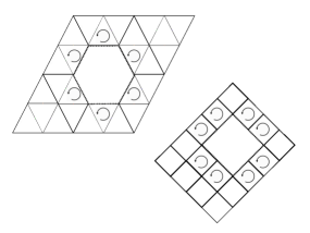
Figure 1: Defects in triangular (left) and square (right) lattices.

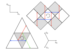
Figure 2: Quantum Walks scheme on triangular (left) and square (right) lattice. On the triangular grid, an anti-clockwise rotation $R$ is implemented by a partial shift $T_{0,\varepsilon}$ (blue) along a direction ${\bf u}_{0}$, $T_{1,\varepsilon}$ (red) along a direction ${\bf u}_{1}$ and $T_{2,\varepsilon}$ (green) along a direction ${\bf u}_{2}$. On the square grid, an anti-clockwise rotation $R$ is implemented by only two partial shifts $T_{x,\varepsilon}$ (blue) along a direction ${\bf u}_{x}$, $T_{y,\varepsilon}$ (red) along a direction ${\bf u}_{y}$.

Remember that a quantum walks (QW) are essentially local unitary gates that drive the evolution of a particle on a lattice. They have been used as a mathematical framework to express many quantum algorithms e.g. BooleanEvalQW ; ConductivityQW , but also many quantum simulation schemes e.g. di2014quantum ; di2016quantum ; ArrighiQED . This is where things get interesting. Indeed, it has been shown that many of these QW admit, as their continuum limit, the Dirac equation bialynicki-birula_weyl_1994 ; meyer_quantum_1996 ; hatifi2019quantum ; di2020quantum , providing ‘quantum simulation schemes’, for the future quantum computers, to simulate all free spin-$1/2$ fermions.

Recall that the Grover search is the alternation of a diffusion step, with an oracle step. Here we provide evidence that 1/ these Dirac QW, in $(2+1)$–dimensions, work fine to implement the diffusion step of the Grover search and 2/ Topological defects also work fine to implement the oracle step of the Grover search.

The second point is, on the practical side, probably more important than the first. Indeed, whilst there are several experimental realizations of QW, including 2D QW, WernerElectricQW ; Tangeaat3174 , these have not been considered as scalable substrates for implementing the Grover search so far—probably due to the lack of an easy way of implementing the oracle step.

From a theoretical perspective, that point is strongly suggestive also. Indeed, recall that many quantum algorithms are formulated as a QW search on a graph, whose nodes represent elements the configuration space of a problem, and whose edges represent the existence of a local transformation between two configurations—see QWSubset for a recent example of that. So far, the QW search has only been used to look for ‘marked nodes’, i.e. good configurations within the configuration space, as specified by an oracle. Here, in contrast, the QW search is used to look for topological defects, which are properties of the configuration space itself. This suggests aiming beyond recognizing simple hole defects in 2D crystals, to target more general topological classification problems—e.g. seeking to characterize homotopy equivalence over configuration spaces that represent manifolds as CW-complexes mermin1979topological ; aschenbrenner2015decision .

I Dirac quantum walks

We consider QW both over the square and the triangular grid. More precisely we consider periodic tilings of the plane, where the tiles are either squares or equilateral triangles, of alternating grey and white colours, as in Fig. 2. The walker lives over the middle points of each side (aka facet) of each tile. For the square grid we can label these points by their positions in $\mathbb{Z}^{2}$, for the triangular grid this would be a subset of $\mathbb{Z}^{2}$. To any such point ${\bf x}$ we assign a complex number representing the amplitude of the walker being there, which we denote by $\psi^{+}({\bf x})$ (resp. $\psi^{-}({\bf x})$) if the tile is white (resp. grey). Of course wherever two facets are glued, so are their middle points, and so the two complex numbers form a spinor $\psi({\bf x})=(\psi^{+}({\bf x})\ \ \psi^{-}({\bf x}))^{\top}$ in $\mathcal{H}_{2}$. Letting $\ket{v_{+}}=(1\ \ 0)^{\top}$ and $\ket{v_{-}}=(0\ \ 1)^{\top}$ we may then write $\psi({\bf x})=\psi^{+}({\bf x})\ket{v_{+}}+\psi^{-}({\bf x})\ket{v_{-}}$. This degree of freedom at a single point is referred to as the walker’s ‘coin’ or ‘spin’. For the full square grid, the overall state of the walker therefore lies in the composite Hilbert space $\mathcal{H}_{2}\otimes\mathcal{H}_{\mathbb{Z}^{2}}$ and can be written $\ket{\psi}=\sum_{{\bf x}}\psi^{-}({\bf x})\ket{v_{-}}\otimes\ket{{\bf x}}+\psi^{+}({\bf x})\ket{v_{+}}\otimes\ket{{\bf x}}$. For the full triangular grid the amplitude of one in every two position needs be zero. For a grid with a missing white (resp. grey) tile the corresponding $\psi^{+}({\bf x})$ (resp. $\psi^{-}({\bf x})$) for ${\bf x}$ on a side of the tile, needs be zero.
The class of evolution operators that we consider in this paper are QW of the form:

$$\ket{\psi(t+\varepsilon/l)}=WR\ket{\psi(t)}$$ (1)

with $l=2$ for the square grid and $l=3$ for the triangular grid. Here, $R$ stands for the synchronous anti-clockwise rotation of all tiles. Notice that, wherever there is no missing tile, the simultaneous rotations of the two tiles glued at ${\bf x}$ precisely coincides with the implementation of a partial shift $T_{k,\varepsilon}$ along a direction ${\bf u}_{k}$:

$$T_{k,\varepsilon}\begin{pmatrix}\psi^{+}({\bf x})\\ \psi^{-}({\bf x})\end{pmatrix}=\begin{pmatrix}\psi^{+}({\bf x}+{\bf u}_{k}\varepsilon)\\ \psi^{-}({\bf x}-{\bf u}_{k}\varepsilon)\end{pmatrix}.$$ (2)

Moreover, $W$ stands for the synchronous application of a $2\times 2$ unitary $W({\bf x})$ on the spins $\psi({\bf x})$. This unitary depends on ${\bf x}$ only in a very simple way which we now clarify. First of all, if it so happens that a tile is missing at ${\bf x}$, then the spinor $\psi({\bf x})$ is incomplete, and so $W({\bf x})=I$. Second of all, if there is no missing tile, then $W({{\bf x}})=W_{k}$, where the $k$ is that corresponding to the partial translation direction ${\bf u}_{k}$ occurring at ${\bf x}$.
It follows that, in the case of a full grid, any given walker will undergo $T_{k,\varepsilon}$ and then $W_{k}$ for $k=0\ldots l-1$ successively, amounting to

$$\ket{\psi(t+\varepsilon)} =W_{\textrm{$l$}-1}T_{\textrm{$l$}-1,\varepsilon}\ldots W_{0}T_{0,\varepsilon}\ket{\psi(t)}$$

$$=\Pi_{k}W_{k}T_{k,\varepsilon}\ket{\psi(t)}.$$ (3)

The way we choose these $W_{k}$ is so that QW is Dirac QW, meaning that

$$\Pi_{k}W_{k}T_{k,\varepsilon}\approx\exp(i\varepsilon H_{D})$$ (4)

as we neglect the second order terms in $\varepsilon$, with $H_{D}$ the Dirac Hamiltonian in natural $\hbar=c=1$ units, i.e.

$$H_{D}=p_{x}\sigma_{x}+p_{y}\sigma_{y}+m\sigma_{z}.$$

Therefore, on the full grid, these QW simulate the Dirac Equation, more and more closely as $\varepsilon$ goes to zero.

Square grid.

Let us consider the unit vectors along the $x$–axis and $y$–axis, namely $\{{\bf u}_{x},{\bf u}_{y}\}$ and use them to specify the directions of the translations $T_{x,\varepsilon}$ and $T_{y,\varepsilon}$. Eq. (3) then reads:

$$U=W_{+}T_{y,\varepsilon}W_{-}T_{x,\varepsilon}$$ (5)

where $W_{\pm}=\exp(i\sigma_{x}\theta_{\pm})$ with $\theta_{\pm}=\pm(\frac{\pi}{4}\pm\varepsilon m)$ and $m$ a is real constant, namely the mass. In the formal limit for $\varepsilon\rightarrow 0$, Eq.(5) recovers the Dirac Hamiltonian in $(2+1)$–spacetime. Iterations of the walk observationally converge towards solutions of the Dirac Eq., as was proven in full rigor in arrighi2014dirac , which motivated the above choice of $U$ on the square grid in the following.

Triangular grid.

For the Triangular grid let us consider the unit vectors $\{{\bf u}_{0},{\bf u}_{1},{\bf u}_{2}\}$, as in Fig. 2 and defined by

$${\bf u}_{k}=\cos\left({\frac{2k\pi}{3}}\right){\bf u}_{x}+\sin\left({\frac{2k\pi}{3}}\right){\bf u}_{y}\hskip 7.11317pt\text{for}\hskip 7.11317ptk=0,1,2.$$ (6)

and use them to specify the directions of the translations $T_{i,\varepsilon}$. Eq. (3) then reads:

$$e^{-i\varepsilon H_{D}}=WT_{2,\varepsilon}WT_{1,\varepsilon}WT_{0,\varepsilon}$$ (7)

with $W=e^{i\frac{\pi}{3}}e^{-i\frac{\alpha}{2}\sigma_{y}}e^{-i\frac{\pi}{3}\sigma_{z}}e^{i\frac{\alpha}{2}\sigma_{y}}e^{-i\varepsilon\frac{3}{\sqrt{5}}m\sigma_{z}}$ the coin operator, which turns out not to depend on the direction ${\bf u}_{k}$. In arrighi_dirac_2018 it has been proved in detail by some of the authors how this particular choice also leads, in the continuum limit, to the Dirac Hamiltonian in $(2+1)$–spacetime, which again motivated us to adopt the above $W$ on the triangular grid in presence of defects.

Defects.

A sector of a crystal lattice may be inaccessible, e.g. due to surface defects such as the vacancy of an atom (e.g. Schottky point defect) and others. These affect the physical and chemical properties of the material, including electrical resistivity or conductivity ibach1995solid . Here we model these defects in the simplest possible way: locally, a small number of squares or triangles are missing, thereby breaking the translational invariance of the lattice. In other words, the walker is forbidden access to a ball $\mathcal{B}$ of unit radius, as in Fig. 1.This is done by reflecting those signals that reach the boundary $\mathcal{\partial B}$ of the ball, simply by letting $W=I$ on the facets around $\mathcal{\partial B}$.

Notice that, wherever we replace the coin $W$ by identity, both Dirac walks reduce to just anti-clockwise rotation $R$ as in Eq. (1), see Fig. 1. Still, the operators (5) and (7) may have different topological properties around $\mathcal{\partial B}$. For instance, the square grid QW has vanishing Chern number and trivial topological properties kitagawa2012topological for vanishing $m$, which can still become non-trivial from $m>0$ asboth2015edge . The triangular walk on the other hand is always topologically non-trivial and has Chern number equal to one kitagawa2010exploring . In the triangular case the positive and negative component decouple respectively in the grey and the white triangles, and may be thought of as inducing polarized local topological currents of spin, called edge states verga2017edge . According to verga2017edge , this phenomenon will be observed whenever initial states have an overlap with $\mathcal{\partial B}$, elsewhere the walker does not localize and explores the lattice with ballistic speed. Thus, we expect these topological effects to become significant in the triangular case and it is indeed the case.

Our conjecture is that, starting from a uniformly superposed wavefunction, the walker will, in finite time, localise around the defect in $O(\sqrt{N})$ steps, with probability in $O(1/\log(N))$, with $N$ the total number of squares/triangles. In the following we discuss the numerical evidence we have for such a conjecture.

II Grover search

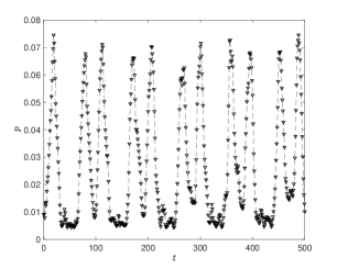
Figure 3: Square grid periodic localization. Probability of being localized around the center of the defect versus time. For $m=0$ and $N=2500$.

Our numerical simulations over the square and triangular grids are exactly in line with a series of results childs2004spatial ; aaronson2003quantum ; tulsi2008faster showing that $2D$ spatial search can be performed in $O(\sqrt{N})$ steps with a probability of success in $O(1/\log{N})$. With $O(\log{N})$ repetitions of the experiment one makes the success probability an $O(1)$, yielding an overall complexity of $O(\sqrt{N}\log{N})$. Making use of quantum amplitude amplification brassard2002quantum , however, one just needs $O(\sqrt{\log{N}})$ repetitions of the experiment in order to make the probability an $O(1)$, yielding an overall complexity of $O(\sqrt{N\log{N}})$. This bound is unlikely to be improved, given the strong arguments given by magniez2012hitting ; santha2008quantum ; patel2010search .
These works were not using Dirac QW, nor defects. Our aim here is demonstrate that QW which recover the Dirac equation, also perform a Grover search, as they propagate over the discrete surface and localise around its defects. More concretely we proceed as follows: (i) Prepare, as the initial state the wavefunction which is uniformly superposed over every square or triangle, and whose coin degree of freedom is also the uniformly superposed $(\ket{v^{+}}+\ket{v^{-}})/\sqrt{2}$. Notice that amplitude inside the defect is zero; (ii) Let the walker evolve with time; (iii) Quantify the number of steps $t(N)$ before the walker reaches its probability peak $p(N)$ of being localized in a ball of radius $2$ around the center of the defect, namely the peak recurrence time and estimate this probability peak, at fixed $N$; (iv) Characterize $t(N)$ and $p(N)$, i.e. the way the peak recurrence time and the probability peak depend upon the total number of squares/triangles $N$.

We indeed observe that the probability of being found around the defect has a periodic behaviour, see in Fig. 3 for the case of the square lattice: for instance with $N=2500$ sites, for $m=0$, the peak recurrence time is at $t\sim 25$, with maximum probability is $p\simeq 10^{-1}$. The dependencies in $N$ were interpolated from the data set, as shown in Fig. 4.a. We observe that $t(N)=\sqrt{N}$ and $p(N)\simeq 1/\log{N}$ asymptotically, with a prefactor that depends on $m$. In this massless case the interpolation $p(N)\simeq 1/\log{N}$ works right-away, but when the mass gets larger, the curve remains longer along a $p(N)\simeq 1/N$ trajectory, before it eventually enters its asymptotic $p(N)\simeq 1/\log{N}$ regime. Moreover, as shown in Fig. 4.b, in presence of more than one topological defects we the way the peak recurrence time and the probability depend upon $N$ is the same. Notice that the prefactors do not depend on the number of defects but only depend on $m$, as shown in Fig. 4.a.

Clearly, repeating the experiment an $O(\log N)$ number of times will make the probability of finding the defect as close to $1$ as desired, leading to an overall time complexity in $O(\sqrt{N}\log N)$. Again we could, instead, propose to use quantum amplitude amplification brassard2002quantum in order to bring the needed number of repetitions down an $O(\sqrt{\log N})$, leading to an overall time complexity in $O(\sqrt{N\log N})$. But it seems that this would defeat the purpose of this paper to some extent: since our aim is to show that there is a ‘natural implementation’ of the Grover search, we must not rely on higher-level routines such as quantum amplitude amplification.

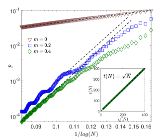
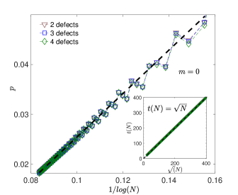
Figure 4: Square grid scalings. (Top) Probability peak of being localized around one defect, versus the number of squares in the grid for different value of the mass $m$. (Bottom) Probability peak of being localized around two, three and four defects respectively, versus the number of squares in the grid for $m=0$. The inset shows the peak recurrence time.

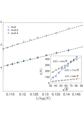
Figure 5: Triangular grid scalings. Recurring probability peak of being localized around the defect, versus the number of triangles in the grid. The inset shows the peak recurrence time.

Over the triangular grid the Grover search is again at play. Indeed the data set of Fig. 5, confirms the results obtained over the square grid: the peak recurrence time is again $t(N)\simeq O(\sqrt{N})$, and its corresponding probability peak is again $p(N)\simeq O(1/\log{N})$ for large $N$, again with a prefactor that depends on the mass. Again this leads to an overall complexity of $O(\sqrt{N}\log{N})$, or $O(\sqrt{N\log{N}})$ using amplitude amplification.

III Conclusion

It is now common knowledge that Quantum Walks (QW) implement the Grover search, and that some QW mimic the propagation of the free 1/2-spin fermion. Yet, could this mean that these particles naturally implement the Grover search? Answering this question positively may be the path to a serious technological leap, whereby experimentalist would bypass the need for a full-fledged scalable and error-correcting Quantum Computer, and take the shortcut of looking for ‘natural occurrences’ of the Grover search instead. So far, however, this idea has remained unexplored. The QW used to implement the Grover diffusion step were unrelated to the Dirac QW used to simulate the 1/2-spin fermion, with the noticeable exception of patel2010search . More crucially, the Grover oracle step seemed like a rather artificial, involved controlled-phase, far from something that could occur in nature. This contribution begins to remedy both these objections.

We used Dirac QW over both the triangular and the square grid as the Grover diffusion step and, instead of alternating this with an extrinsic oracle step, we coded for the solution directly inside the grid, by introducing a topological defect. We obtained strong numerical evidence showing that the Dirac QW localize around the defect in $O(\sqrt{N})$ steps with probability $O(1/\log{N})$, just like previous QW search would. Our next step is to use QW to locate not just a hole defect, but a particular QR code–like defect, amongst many possible others that could be present on the lattice. This would bring us one step closer to a natural implementation of an unstructured database Grover search. Replacing the Grover oracle step by surface defects seems way more practical in terms of experimental realizations, whatever the substrate, possibly even in a biological setting patel2011efficient . At a more abstract level, this suggests using QW to search, not just for ’good’ configurations within a space, but rather for topological properties of the configuration space itself.

Acknowledgements

The authors acknowledge inspiring conversations with Fabrice Debbasch, that sparked the idea of Grover searching for surface defects; enlightening discussions on topological effects with Alberto Verga; and useful remarks on how to better present this work by Janos Asboth, Tapabrata Ghosh, Apoorva Patel and the anonymous referees. This work has been funded by the Pépinière d’Excellence 2018, AMIDEX fondation, project DiTiQuS and the ID# 60609 grant from the John Templeton Foundation, as part of the “The Quantum Information Structure of Spacetime (QISS)” Project.

- [1] Scott Aaronson and Andris Ambainis. Quantum search of spatial regions. In 44th Annual IEEE Symposium on Foundations of Computer Science, 2003. Proceedings., pages 200–209. IEEE, 2003.
- [2] Andris Ambainis, Andrew M Childs, Ben W Reichardt, Robert Špalek, and Shengyu Zhang. Any and-or formula of size n can be evaluated in time n^1/2+o(1) on a quantum computer. SIAM Journal on Computing, 39(6):2513–2530, 2010.
- [3] Pablo Arrighi, Cédric Bény, and Terry Farrelly. A quantum cellular automaton for one-dimensional qed. Quantum Information Processing, 19(3):88, 2020.
- [4] Pablo Arrighi, Giuseppe Di Molfetta, Iván Márquez-Martín, and Armando Pérez. The Dirac equation as a quantum walk over the honeycomb and triangular lattices. Physical Review A, 97(6):062111, June 2018. arXiv: 1803.01015.
- [5] Pablo Arrighi, Vincent Nesme, and Marcelo Forets. The dirac equation as a quantum walk: higher dimensions, observational convergence. Journal of Physics A: Mathematical and Theoretical, 47(46):465302, 2014.
- [6] Janos K Asboth and Jonathan M Edge. Edge-state-enhanced transport in a two-dimensional quantum walk. Physical Review A, 91(2):022324, 2015.
- [7] Matthias Aschenbrenner, Stefan Friedl, and Henry Wilton. Decision problems for 3–manifolds and their fundamental groups. Geometry & Topology Monographs, 19(1):201–236, 2015.
- [8] Iwo Bialynicki-Birula. Weyl, Dirac, and Maxwell equations on a lattice as unitary cellular automata. Physical Review D, 49(12):6920–6927, June 1994.
- [9] Xavier Bonnetain, Rémi Bricout, André Schrottenloher, and Yixin Shen. Improved classical and quantum algorithms for subset-sum. arXiv preprint arXiv:2002.05276, 2020.
- [10] Gilles Brassard, Peter Hoyer, Michele Mosca, and Alain Tapp. Quantum amplitude amplification and estimation. Contemporary Mathematics, 305:53–74, 2002.
- [11] Filippo Cardano, Alessio D’Errico, Alexandre Dauphin, Maria Maffei, Bruno Piccirillo, Corrado de Lisio, Giulio De Filippis, Vittorio Cataudella, Enrico Santamato, Lorenzo Marrucci, et al. Detection of zak phases and topological invariants in a chiral quantum walk of twisted photons. Nature communications, 8(1):1–7, 2017.
- [12] Andrew M Childs and Jeffrey Goldstone. Spatial search by quantum walk. Physical Review A, 70(2):022314, 2004.
- [13] Giuseppe Di Molfetta and Pablo Arrighi. A quantum walk with both a continuous-time limit and a continuous-spacetime limit. Quantum Information Processing, 19(2):47, 2020.
- [14] Giuseppe Di Molfetta, Marc Brachet, and Fabrice Debbasch. Quantum walks in artificial electric and gravitational fields. Physica A: Statistical Mechanics and its Applications, 397:157–168, 2014.
- [15] Giuseppe Di Molfetta and Armando Pérez. Quantum walks as simulators of neutrino oscillations in a vacuum and matter. New Journal of Physics, 18(10):103038, 2016.
- [16] Maximilian Genske, Wolfgang Alt, Andreas Steffen, Albert H Werner, Reinhard F Werner, Dieter Meschede, and Andrea Alberti. Electric quantum walks with individual atoms. Physical review letters, 110(19):190601, 2013.
- [17] Lov K. Grover. A fast quantum mechanical algorithm for database search. In Proceedings of the twenty-eighth annual ACM symposium on Theory of computing - STOC ’96, pages 212–219, Philadelphia, Pennsylvania, United States, 1996. ACM Press.
- [18] Mohamed Hatifi, Giuseppe Di Molfetta, Fabrice Debbasch, and Marc Brachet. Quantum walk hydrodynamics. Scientific reports, 9(1):2989, 2019.
- [19] Harald Ibach and Hans Lüth. Solid-State Physics: An Introduction to Theory and Experiment. Springer-Verlag, 1995.
- [20] Takuya Kitagawa. Topological phenomena in quantum walks: elementary introduction to the physics of topological phases. Quantum Information Processing, 11(5):1107–1148, 2012.
- [21] Takuya Kitagawa, Mark S Rudner, Erez Berg, and Eugene Demler. Exploring topological phases with quantum walks. Physical Review A, 82(3):033429, 2010.
- [22] Frédéric Magniez, Ashwin Nayak, Peter C Richter, and Miklos Santha. On the hitting times of quantum versus random walks. Algorithmica, 63(1-2):91–116, 2012.
- [23] N David Mermin. The topological theory of defects in ordered media. Reviews of Modern Physics, 51(3):591, 1979.
- [24] David A. Meyer. From quantum cellular automata to quantum lattice gases. Journal of Statistical Physics, 85(5-6):551–574, December 1996. arXiv: quant-ph/9604003.
- [25] Apoorva Patel, KS Raghunathan, and Md Aminoor Rahaman. Search on a hypercubic lattice using a quantum random walk. ii. d= 2. Physical Review A, 82(3):032331, 2010.
- [26] Apoorva D Patel. Efficient energy transport in photosynthesis: Roles of coherence and entanglement. In AIP Conference Proceedings, volume 1384, pages 102–107. AIP, 2011.
- [27] A. Romanelli, A. Auyuanet, and R. Donangelo. Quantum search with resonances. Physica A: Statistical Mechanics and its Applications, 360(2):274 – 284, 2006.
- [28] Miklos Santha. Quantum walk based search algorithms. In International Conference on Theory and Applications of Models of Computation, pages 31–46. Springer, 2008.
- [29] Hao Tang, Xiao-Feng Lin, Zhen Feng, Jing-Yuan Chen, Jun Gao, Ke Sun, Chao-Yue Wang, Peng-Cheng Lai, Xiao-Yun Xu, Yao Wang, Lu-Feng Qiao, Ai-Lin Yang, and Xian-Min Jin. Experimental two-dimensional quantum walk on a photonic chip. Science Advances, 4(5), 2018.
- [30] Avatar Tulsi. Faster quantum-walk algorithm for the two-dimensional spatial search. Physical Review A, 78(1):012310, 2008.
- [31] Alberto D Verga. Edge states in a two-dimensional quantum walk with disorder. The European Physical Journal B, 90(3):41, 2017.
- [32] Guoming Wang. Efficient quantum algorithms for analyzing large sparse electrical networks. Quantum Info. Comput., 17(11-12):987–1026, September 2017.
- [33] L Xiao, X Zhan, ZH Bian, KK Wang, X Zhang, XP Wang, J Li, K Mochizuki, D Kim, N Kawakami, et al. Observation of topological edge states in parity–time-symmetric quantum walks. Nature Physics, 13(11):1117–1123, 2017.