Non-parametric Morphologies of Galaxies in the eagle Simulation

Abstract

We study the optical morphology of galaxies in a large-scale hydrodynamic cosmological simulation, the eagle simulation. Galaxy morphologies were characterized using non-parametric statistics (Gini, $M_{20}$, Concentration and Asymmetry) derived from mock images computed using a 3D radiative transfer technique and post-processed to approximate observational surveys. The resulting morphologies were contrasted to observational results from a sample of $\log_{10}(M_{*}/\textnormal{M}_{\odot})>10$ galaxies at $z\sim 0.05$ in the gama survey. We find that the morphologies of eagle galaxies reproduce observations, except for asymmetry values which are larger in the simulated galaxies. Additionally, we study the effect of spatial resolution in the computation of non-parametric morphologies, finding that Gini and Asymmetry values are systematically reduced with decreasing spatial resolution. Gini values for lower mass galaxies are especially affected. Comparing against other large scale simulations, the non-parametric statistics of eagle galaxies largely agree with those found in IllustrisTNG. Additionally, eagle galaxies mostly reproduce observed trends between morphology and star formation rate and galaxy size. Finally, We also find a significant correlation between optical and kinematic estimators of morphologies, although galaxy classification based on an optical or a kinematic criteria results in different galaxy subsets. The correlation between optical and kinematic morphologies is stronger in central galaxies than in satellites, indicating differences in morphological evolution.

1 Introduction

Galaxy morphology is not only important for classification, it also provides crucial information on the evolution of galaxies. This is justified by the fact that morphology is found to be strongly linked to the local environment (Dressler, 1984; Gómez et al., 2003; Blanton & Moustakas, 2009; Kormendy et al., 2010), merger history (Lotz et al., 2008a), stellar mass (Kauffmann et al., 2003; Ilbert et al., 2010) and star formation history (Kauffmann et al., 2003; Baldry et al., 2004; Bell et al., 2012) of a galaxy. See also Conselice (2014) for a recent review on the topic. In the last decade, large galaxy surveys have established the existence of a bimodality in the nearby Universe where star-forming galaxies exhibit disc-dominated (late-type) morphologies, while quiescent galaxies exhibit bulge-dominated (early-type) morphologies. However, the detailed origin of the observed distribution of morphologies is still debated, since the complete physics of quenching and the assembly history of bulges is not yet fully understood.

Numerical simulations offer unique insight into this problem because they can link the morphology of a galaxy to the underlying physical processes that gave rise to it in the first place. It is therefore desirable to be able to robustly map the results of the simulations to morphological measurements that can be contrasted to observations. A particularly powerful way to achieve this consists in the generation and subsequent analysis of mock galaxy images from hydrodynamic simulations. Several codes now exist that can produce such images: sunrise (Jonsson, 2006), hyperion (Robitaille, 2011), and skirt (Baes et al., 2011; Camps & Baes, 2015). These codes model the propagation of photons trough the interstellar medium (ISM) and the effects of dust absorption and scattering by solving the three-dimensional radiative transfer calculations (e.g. Steinacker et al., 2013) using Monte Carlo techniques (e.g. Whitney, 2011)

A key advantage of the use of mock images is that morphological analysis can be performed in the same way in simulations and observations, using all of the currently available techniques: non-parametric statistics (e.g. Lotz et al., 2008a; Snyder et al., 2015b; Snyder et al., 2015a; Bignone et al., 2017; Rodriguez-Gomez et al., 2019); bulge/disc decompositions based on Sérsic indexes (Scannapieco et al., 2010; Bottrell et al., 2017); human-based visual classification (Dickinson et al., 2018) and machine learning algorithms (Pearson et al., 2019; Huertas-Company et al., 2019).

Non-parametric morphologies (Lotz et al., 2004; Conselice et al., 2000; Freeman et al., 2013; Pawlik et al., 2016) play a central role because they are generally more flexible than classifications based on Sérsic index, i.e. they can be used even in cases of irregular morphologies (Lotz et al., 2008b). Also, they are generally easier to obtain, quantify and interpret than human- or machine- based visual classification, although they do not provide as detailed morphological taxonomies. All things considered, they provide a robust way to compare the visual morphologies of observations and simulations.

In this work we study the optical morphologies of galaxies in the eagle simulations (Schaye et al., 2015; Crain et al., 2015; McAlpine et al., 2016) at $z=0.1$. To do so, we use non-parametric statistics to quantify the light distribution of mock galaxy images obtained using the radiative transfer code skirt (Camps et al., 2016; Trayford et al., 2017), which include modelling of dust absorption and scattering and that have been post-processed to mimic SDSS and LSST images. We apply the same characterization techniques to SDSS observations of galaxies in the gama survey and compare our results. We also contrast the morphologies of eagle galaxies with that of other large-scale simulations: Illustris (Nelson et al., 2015; Vogelsberger et al., 2014) and IllustrisTNG (Nelson et al., 2019; Pillepich et al., 2018b; Springel et al., 2018; Nelson et al., 2018; Naiman et al., 2018; Marinacci et al., 2018). This work also complements other related studies based on the eagle simulations that characterize morphologies based on kinematic properties (Correa et al., 2017; Correa et al., 2019; Lagos et al., 2018; Clauwens et al., 2018; Rosito et al., 2018a) or the combination of kinematics and the spatial distribution of stellar mass (Trayford et al., 2019; Thob et al., 2019).

This paper is organized as follows. In Section 2 we describe the simulations used in this work and the simulated and observational galaxy samples we characterize morphologically. In Section 3 we describe the procedures used to obtain the simulated and observational galaxy images and to derive the non-parametric statistics. We present our main results in Section 4. Finally, we summarize and discuss these results in Section 5.

2 Simulation and data

2.1 The eagle Simulations

The eagle simulations (Crain et al., 2015; Schaye et al., 2015) are a suite of cosmological hydrodynamic simulations run with a modified version of the Gadget-3 N-Body Tree-PM smoothed particle hydrodynamics (SPH) code, which is an updated version of Gadget-2 (Springel, 2005). The simulations follow the evolution of gas and dark matter in periodic cubic volumes, with a range of resolutions and different parameter sets for the subgrid models. The physics described by these subgrid models include the heating and cooling of gas (Wiersma et al., 2009a), star formation (Schaye & Dalla Vecchia, 2008), stellar mass loss (Wiersma et al., 2009b), energy feedback from star formation (Dalla Vecchia & Schaye, 2012) and active galactic nuclei (AGN) feedback (Rosas-Guevara et al., 2015). The model parameters regulating the energy feedback from star formation and AGNs were calibrated so as to reproduced the observed galaxy stellar mass function (GSMF) at $z\sim 0$. Additionally, a dependence of the stellar feedback energy on the gas density was introduced so as to reproduce the galaxy mass-size relation at $z\sim 0.1$. A comprehensive description of the calibration procedure can be found in Crain et al. (2015).

Star formation is treated stochastically in eagle using a pressure-dependent formulation of the empirical Kennicutt–Schmidt law following (Schaye & Dalla Vecchia, 2008) but with a metallicity-dependent density threshold (Schaye, 2004). Gas particles that are converted into stars inherit the chemical abundance of their parent and are treated as single stellar population, assuming a Chabrier (2003) stellar initial mass function (IMF). These stellar populations lose mass through stellar winds and are subjected to mass loss via Type Ia and Type II supernovae events which result in the chemical enrichment of their surrounding gas particles (Wiersma et al., 2009b). Abundances for eleven individual elements (H, He, C, N, O, Ne, Mg, Si, S, Ca and Fe) are followed in the simulations.

In this work, we concentrate our analysis on the reference model (Ref) run in a cosmological volume of 100 comoving Mpc on a side (Ref100N1504, hereafter Ref-100). Additionally, in appendix B we analyse two smaller volumes, 25 comoving Mpc a side (RefL025N0376 and RecalL025N0752), to test the numerical convergence of non-parametric statistics. Key properties of the eagle simulations used in this work are listed in table 1.

Table 1: Parameters of the eagle and Illustris simulations used in this work. From left to right: simulation identifier, side length of cubic volume L in co-moving Mpc (cMpc), gas particle initial mass $m_{\textnormal{g}}$, Plummer equivalent gravitational softening $\epsilon_{\textnormal{prop}}$ at redshift z = 0 in proper kpc (pkpc)

Name	$L$	$m_{\textnormal{g}}$	$\epsilon_{\textnormal{prop}}$
	cMpc	$10^{5}$ M⊙	pkpc
Ref100N1504 (Ref-100)	100	$18.1$	0.70
RefL025N0376 (Ref-25)	25	$18.1$	0.70
RecalL025N0752 (Recal-25)	25	$2.26$	0.35
Illustris-1 (Illustris)	106.5	$12.6$	0.71
TNG100-1 (IllustrisTNG)	110.7	$13.9$	0.74

The cosmological parameters assumed by the eagle simulations are those inferred by the Planck Collaboration et al. (2014), the key parameters being $\Omega_{m}=0.307$, $\Omega_{\Lambda}=0.693$, $\Omega_{b}=0.04825$, $h=0.6777$ and $\sigma_{8}=0.8288$. We adopt the same cosmological parameters for this work.

2.2 Simulated galaxy samples

2.2.1 Ref-100

Dark matter haloes in eagle are identified using the friends-of-friends (FoF) algorithm (Davis et al., 1985) with a linking length of $b=0.2$ times the inter particle separation. Particles representing gas, stars and BHs are associated with the FoF group of their nearest dark matter particle. Self-bound substructures (subhalos) comprising dark matter, stars and gas are then identified using the subfind algorithm (Springel et al., 2001). Each simulated galaxy is associated with an individual subhalo.

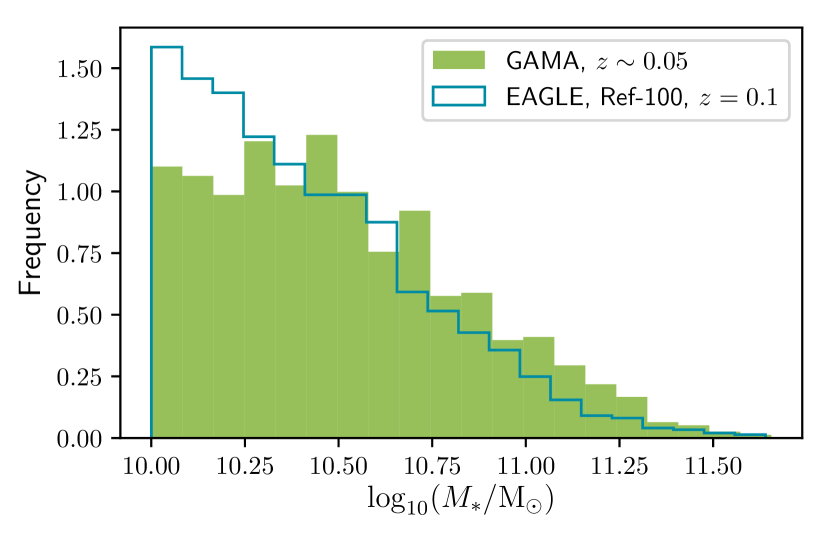
Figure 1: Stellar mass distribution of the gama and Ref-100 samples. The gama sample presents a slightly higher median stellar mass of $10^{10.45}$ M_⊙ compared to the median stellar mass of $10^{10.36}$ M_⊙ in the Ref-100 sample due to the paucity of galaxies below $\sim 10^{10.5}$ M_⊙. See text for a more complete discussion

We focus our study in galaxies in a single snapshot (snapshot 27) at $z=0.1$ with $M_{*}>10^{10}$ M_⊙, the same galaxy sample for which images were produced by Trayford et al. (2017) using skirt. The resulting mock catalogue includes 3624 galaxies with most galaxies being resolved by more than $10000$ stellar particles. The lowest number of stellar particle for a galaxy in this sample is 6710. The sample contains 2255 (62%) central and 1369 (38%) satellite galaxies. A summary of the properties of this simulated galaxy sample can be found in table 2.

Unless otherwise stated, all integrated galaxy properties (i.e. stellar mass, star formation rate, half-light radius) in this sample are computed using spherical apertures of 30 pkpc positioned on the centre of potential of the corresponding galaxy.

2.2.2 Illustris and IllustrisTNG

It is particularly interesting to compare our results with those obtained using other cosmological simulations. This comparison can serve to illustrate similarities and differences in the morphologies of simulated galaxies produced by the different modelling of the physics of galaxy formation. Currently, Illustris and IllustrisTNG are the two simulation suites that provide the kind of non-parametric morphological studies that are directly comparable to this work.

Both Illustris and IllustrisTNG are a series of hydrodynamic cosmological simulations run with the moving-mesh code AREPO, with IllustrisTNG featuring an updated version of the Illustris galaxy formation model (Vogelsberger et al., 2013; Torrey et al., 2014). The main ways in which IllustrisTNG differs from the original Illustris are the inclusion of ideal magneto-hydrodynamics, a new AGN feedback model that operates at low accretion rates (Weinberger et al., 2017) and modifications to the galactic winds, stellar evolution and chemical enrichments according to Pillepich et al. (2018a).

In this study we use data from the highest resolution version of ‘TNG100’, hereafter IllustrisTNG and from the original ‘Illustris 1’ simulation, hereafter Illustris. Both simulations are very similar in terms of simulated volume and resolution and differ mainly in the galaxy formation model. Basic Properties for both simulations are detailed in Table 1.

We use non-parametric morphologies of galaxies extracted from Snyder et al. (2015b) and from Rodriguez-Gomez et al. (2019) corresponding to results from Illustris and IllustrisTNG respectively. Additionally, for Illustris, we use asymmetries from Bignone et al. (2017). In all cases we impose a stellar mass threshold of $M_{*}>10^{10}$ M_⊙, matching the Ref-100 sample. This results in a sample of $7024$ ($5926$) galaxies for Illustris (IllustrisTNG).

2.3 The observational galaxy sample

We consider galaxies in the Galaxy And Mass Assembly (gama) survey (Driver et al., 2009; Robotham et al., 2010; Driver et al., 2011), a spectroscopic and multiwavelength survey of five sky fields carried out using the AAOmega multi-object spectrograph on the Anglo-Australian Telescope. The survey has obtained $300000$ galaxy redshifts to $r<19.8$ mag over $\sim 286$ deg², with the survey design aimed at providing uniform spatial completeness. The gama survey provides us with a uniform galaxy database and a comprehensive set of measure properties at low redshift that makes it ideal for comparison with our simulated samples.

Table 2: Properties of the simulated and observational galaxy samples used in this work: From left to right: designation, median stellar mass $\log_{10}$(<M_∗>), redshift, number of galaxies in the sample N. For simulations, the listed redshifts represent the redshift from which the sample was extracted

Sample	$\log_{10}$(<M∗/M⊙>)	Redshift	N
eagle Ref-100	${10.36}$	$0.1$	3624
eagle Ref-25	${10.35}$	$0.1$	70
eagle Recal-25	${10.26}$	$0.1$	75
Illustris	${10.39}$	$0.0$	7024
IllustrisTNG	${10.43}$	$0.05$	5926
gama	${10.45}$	$0.045<z<0.06$	944

Comparisons between eagle and gama galaxies have been carried out in several occasions, including during the calibration procedure mentioned in section 2.1, where the observed GSMF and size–mass relation at $z\sim 0.1$ was used to determine the feedback model parameters (Schaye et al., 2015; Crain et al., 2015). This means that neither the GSMF nor the galaxy sizes can be presented as predictions of the simulations at this redshift. The morphologies of galaxies have not been taken into consideration on the calibration procedure and can therefore be contrasted fairly with gama, or other similar galaxy samples to determine if the simulation reproduces morphologies and what factors contribute to the establishment of optical morphology. Previously, eagle galaxy colours from mock skirt images were also compared with the gama colour-mass diagram by Trayford et al. (2017). They found that optical SKIRT galaxy colours matched observations well and that the modelling by skirt of the scattering and absorption effects of dust improved the agreement with observations, compared to more simple dust-screen models (Trayford et al., 2015).

In this work, we make use of a galaxy subsample derived from the three gama equatorial fields, dubbed G09, G12 and G15, and restricted in redshift and stellar mass. The photometrically derived stellar mass estimates are taken from version 19 of the gama stellar mass catalogue (internal designation StellarMasses) which were computed according to Taylor et al. (2011), corrected for aperture and re-scaled to the eagle cosmology. Spectroscopic redshifts are provided by the StellarMasses catalogue. We restrict our sample to galaxies with stellar mass $M_{*}>10^{10}$ M_⊙ to match the simulated mass range (Section 2.2) and with redshifts in the interval $0.045<z<0.06$ (median redshift $\sim 0.05$), resulting in a total of 944 galaxies. The narrow redshift band allows us to compare morphologies in the observed and simulated samples without considering the effects of evolution in the galaxy population. The median redshift at 0.05 was chosen to match previous works on simulated galaxy morphologies (Snyder et al., 2015b; Bignone et al., 2017; Dickinson et al., 2018; Rodriguez-Gomez et al., 2019). Additionally, this redshift represents the limit at which the resolution of SDSS imaging starts to have a significant impact on the reliability of standard non-parametric morphologies (we analyse image resolution effects in more detail in section 4.3). A summary of the properties of this observational sample can be found in Table 2.

Figure 1 compares the stellar mass distribution of galaxies in the simulated and observational samples. It illustrates the similarities and differences between both galaxy populations. A flattening around and below $10^{10.5}$ M_⊙ can be appreciated in the gama sample which corresponds to the same feature in the GSMF discussed in Baldry et al. (2012). While Ref-100 does not show a similar flattening, the general shape of the GSMF agrees with observations to $\lesssim 0.2$ dex for the full mass range for which the simulation resolution is adequate, i.e. from $2\times 10^{8}$ M_⊙ to over $10^{11}$ M_⊙ (Schaye et al., 2015). Given that uncertainties in the stellar evolution models used to infer stellar masses are $\sim 0.3$ dex (e.g. Conroy et al., 2009), we can consider that the distribution of stellar masses in both samples are comparable for the purposes of this work. The paucity of galaxies towards the lower end of the mass range in the gama sample results in a slightly higher median mass of $10^{10.45}$ M_⊙, compared to the median stellar mass of $10^{10.36}$ M_⊙ in the Ref-100 sample.

We obtain morphological information for our observational sample by cross referencing all objects with the catalogue presented by Domínguez Sánchez et al. (2018). This catalogue provides morphologies for $\sim 600000$ galaxies based in the T-Type classification (de Vaucouleurs, 1963) and in the Galaxy Zoo 2 (GZ2) classification scheme. To achieve that task, they combined existing visual classification catalogues with Convolutional Neural Networks (CNNs) achieving $>97\%$ accuracy for GZ2 morphologies, as well as no offset and a scatter comparable to typical expert visual classifications for T-type morphologies.

3 Image Analysis

3.1 Simulated galaxy images

For galaxies in our simulated sample, we utilize the mock images presented in Trayford et al. (2017) and generated using the radiative transfer code skirt. Here, we summarize the most relevant aspects of the image generation procedure, but interested readers are recommended to refer to the original paper for details.

The skirt Monte Carlo code works by computing the absorption and scattering of monochromatic photon packets from their origin at luminous sources to their destination at a user-defined detector. It is possible to define imaging detectors with a set distance from the source, field of view (FOV) and number of pixels. Datacubes are produced by adding the flux at the position of each pixel separately for each of the wavelengths sampled by the photon packets. Broadband images can then be constructed by convolving the datacubes with the desired filters.

In this paper, we only consider the mass distribution associated with individual subhalos (either centrals or satellites), leaving out close companions and other members of the same halo. This makes the determination of morphologies for individual galaxies robust. The effect of contamination from close companions or background and foreground galaxies are not included in the mock images. Finally, only stellar and gas particles within 30 pkpc of the galaxy centre are considered, a choice initially made in Trayford et al. (2015) to reasonably approximate a Petrosian aperture, but which leaves out some of the light distribution at the outskirts of the most extended galaxies.

3.1.1 Photon sources

Star particles representing stellar populations are used as the sources of the photon packets. The number of photons in each wavelength of the spectral grid is determined by assuming a spectral energy distribution (SED). There are different types of SEDs assigned depending on stellar age. Old stellar populations (age $>10$ Myr) are assigned a galaxev (Bruzual & Charlot, 2003) SED as described in Trayford et al. (2015) and assumed to have a Chabrier (2003) IMF in the [$0.1-100$] M_⊙ mass range. Young stellar populations (age $<10$ Myr) are treated differently because the inability of the simulation to resolve the sub-kpc birth clouds were these stars are embedded. For these stars, the mappings-iii spectral models of Groves et al. (2008) are used, which include dust absorption within the photodissociation region (PDR). Additionally, a re-sampling of stellar and star-forming gas particles is carried out to to mitigate the effects of coarse sampling due to the limited mass resolution (similar to Trayford et al., 2015). Under this procedure, recent star formation is re-sampled in time over the past 100 Myr. Stellar populations re-sampled with ages younger than $10$ Myr are treated with the mappings-iii spectral models, while those with ages older than $>10$ Myr with the galaxev models.

The point of emission of individual photons is determined by randomly sampling truncated Gaussian distributions centred at the position of stellar sources and characterized by a smoothing length. This serves to represent the fact that particles in the simulation do not correspond to individual point sources, but mass distributions instead. Here the distance to the 64th nearest neighbouring star was used as the smoothing length (similar to Torrey et al., 2015). In general terms, the choice of smoothing length has an impact on the appearance of the images, resulting in excessive granularity or oversmoothing and therefore, can have an impact on non-parametric morphologies.

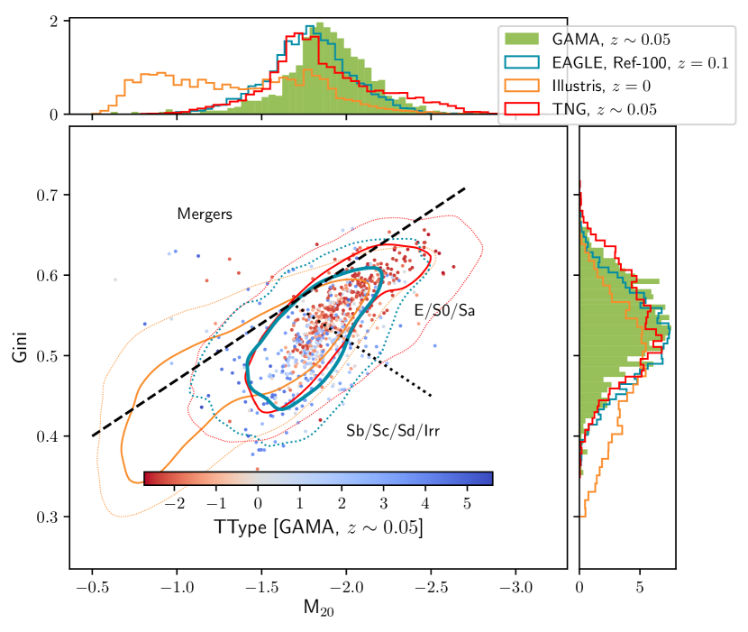
Figure 2: The central panel shows the $G$-M₂₀ diagram from galaxies in Ref-100 (blue), Illustris (orange), IllustrisTNG (red) and gama (points). The coloured solid (dotted) lines enclose regions containing 68 (95) percent of galaxies in each respective sample. The gama galaxies are coloured according to their T-Types. The black dashed and dotted lines separate the subspace into regions for mergers, late types and early types according to Lotz et al. (2008b). We find that Ref-100 and IllustrisTNG have very similar distributions in $G$-M₂₀ space and that they both match gama observations. The top and right panels show respectively the $G$ and M₂₀ normalized distributions for all samples.

3.1.2 Dust modelling

Dust can have an important impact on the appearance of galaxies and is therefore important to account for its effects. In this work, the distribution of dust in the diffuse ISM is approximated by the distribution of gas within the simulation. Since dust is observed to trace the cold metal-rich gas in observed galaxies (e.g. Bourne et al., 2013), a constant dust-to-metal mass ratio is assumed (Camps et al., 2016)

$$f_{\textnormal{dust}}=\frac{\rho_{\textnormal{dust}}}{Z\rho_{g}}=0.3,$$ (1)

where $Z$ is the (SPH-smoothed) metallicity, and $\rho_{\textnormal{dust}}$ and $\rho_{g}$ are the dust and gas density, respectively. Only non star-forming and cold ($T<8000K$) gas contributes to the dust budget.

The dust density is mapped to an adaptively refined (AMR) grid with a minimum cell size of $0.11$ kpc, close to the spatial resolution of eagle. skirt then computes optical depths of each cell at a given reference wavelength and the resulting obscuration. Dust composition is assumed to follow the model described by Zubko et al. (2004); a multicomponent dust mix tuned to reproduce the abundance, extinction and emission constraints of the Milky Way.

3.1.3 Realistic images

The initial datacubes produced for our simulated galaxy sample span $256\times 256$ spatial pixels and 333 wavelengths in the range $0.28-2.5$ $\mu$m, chosen to sample the rest-frame ugrizYJHK photometric bands. Each datacube slice covers a $60\times 60$ kpc area. The camera location is set at 10 Mpc from the galaxy, which results in a pixel scale of $\sim 235$ pc, sufficiently small to simulate SDSS and LSST images for sources at $z>0.02$. The images correspond to a random orientation with respect to the galaxy (but fixed to the $xy$ plane of the simulation box).

We concentrate our morphological analysis on rest-frame broadband g-band, SDSS images obtained by convolving the datacubes in the wavelength dimension with the corresponding filter transmission curve (Doi et al., 2010).

We then follow a procedure very similar to that of Snyder et al. (2015b) to transform the noise-free, ideal images, into realistic images comparable to SDSS observations at $z\sim 0.05$. The procedure can be summarized as follows:

• We first convolve each image with a Gaussian point-spread function (PSF) with a full width at half-maximum (FWHM) of 1 kpc. At $z=0.05$ this approximates the effect of a 1 arcsec seeing, which roughly matches that of SDSS. Alternatively, the resulting mock images can also be comparable to more distant HST imaging at $z=0.5$. We explore other values for the FWHM to study the effect of seeing on non-parametric morphologies in Section 4.3.

• Next, we rebin the image to a constant pixel scale of $0.24$ kpc pixel^-1, which again, roughly matches SDSS imaging.

• Finally, we add Gaussian noise to the images such that the average signal-to-noise ratio of each galaxy pixel is 25. Therefore, we simulate only strongly detected galaxies with morphological measurements not affected by noise.

Also shown through this paper, for illustration purposes, are three-colour gri images based on the ugriz SDSS bands and computed via the approach of Lupton et al. (2004). These images correspond to those publicly available in the eagle database (McAlpine et al., 2016) and have not been degraded in the manner described above.

3.2 Observational sample images

For each galaxy in our gama sample, we downloaded g-band SDSS images from the online Data Release 12 (DR12) archive. We made use of the mosaic tool and the SWarp tool (Bertin et al., 2002) to obtain images centred at the position of the object and restricted to an area $60\times 60$ kpc at the corresponding redshift, matching the limit imposed in our mock images.

The images are sky-subtracted and have a constant pixel scale of $0.396$ arcsec pixel^-1, which is equivalent to $\sim 0.396$ kpc pixel^-1 at the median $z=0.05$ redshift of the sample.

3.3 Structural measurements

To compute non-parametric morphologies of both simulated and observational samples, we use statmorph, a Python package especially developed for this task and used to compute optical morphologies of galaxies in the IllustrisTNG simulation (Rodriguez-Gomez et al., 2019). We concentrate on the computation of Gini ($G$), M₂₀, Concentration ($C$) and Asymmetry ($A$), although the code also allows for the determination of additional morphological parameters.

Details regarding the specific computation of the non-parametric morphologies can be found in Rodriguez-Gomez et al. (2019), the implementation is largely based on Lotz et al. (2004) for the case of $G$-M₂₀ and Conselice (2003) for $C$ and $A$. Here we give a brief summary of how each statistic is measured

3.3.1 Gini

The Gini coefficient is a statistical tool that measures the distribution of a quantity among a population, In the case of galaxy structure, it measures the distribution of light among the pixels that encompass the galaxy image (Lotz et al., 2004); higher values indicate a very unequal distribution (light is mostly concentrated in a few pixels), whereas a lower value indicates a more even distribution. The value of $G$ is defined by the Lorentz curve of the galaxy’s light distribution according to

$$\textnormal{G}=\frac{1}{|\bar{f}|n(n-1)}\sum_{i}^{n}{(2i-n-1)f_{i}},$$ (2)

where $f_{i}$ are a set of $n$ pixel flux values, $i$ ranges from 0 to $n$ and $\bar{f}$ is the average pixel flux value. At the extremes, a value of $G$ = 1 is obtained when all of the flux is concentrated in a single pixel, while $G$ = 0 results from a totally homogeneous flux distribution.

3.3.2 $M_{20}$

The second-order moment parameter, $M_{20}$ gives a value that indicates whether light is concentrated within an image. However, unlike the $C$ statistic, which we define later, $M_{20}$ does not necessarily imply a central concentration. Instead, light could be concentrated in any location in a galaxy. Specifically, the value of $M_{20}$ is the moment of the fluxes of the brightest 20 per cent of light in a galaxy, which is then normalized by the total light moment for all pixels ($M_{\textnormal{tot}}$) (Lotz et al., 2004). $M_{\textnormal{tot}}$ is given by

$$M_{\textnormal{tot}}=\sum_{i}^{n}{M_{i}}=\sum_{i}^{n}{f_{i}[(x_{i}-x_{c})^{2}+(y_{i}-y_{c})^{2}]},$$ (3)

where $f_{i}$ are the pixel flux values and ($x_{c}$, $y_{c}$) is the galaxy’s centre.

$M_{20}$ is then obtained by sorting the pixels by flux and summing $M_{i}$ over the brightest pixels until the sum of the brightest pixels equals 20 per cent of the galaxy’s total flux

$$M_{20}=\log_{10}{\frac{\sum{M_{i}}}{M_{\textnormal{tot}}}},\textnormal{while}\sum_{i}{f_{i}}<0.2f_{n}$$ (4)

3.3.3 Concentration

The $C$ statistic quantifies how much light is in the centre of a galaxy as opposed to its outer parts. It is usually defined (Conselice et al., 2000) as

$$\textnormal{$C$}=5\times\log_{10}{\frac{r_{80}}{r_{20}}},$$ (5)

where $r_{20}$ and $r_{80}$ are the radii of apertures containing 20 and 80 per cent of the total flux, respectively. In the implementation of statmorph, the total flux is measured within a 1.5 petrosian radius and the centre of the aperture corresponds to the point that minimizes the $A$ index.

3.3.4 Asymmetry

Asymmetry is obtained by subtracting the galaxy image rotated by 180^∘ from the original image (Conselice et al., 2000). It is given by

$$\textnormal{$A$}=\frac{\sum_{i,j}{|f_{ij}-f_{ij}^{180}|}}{\sum_{i,j}{|f_{ij|}}}-A_{0},$$ (6)

where $f_{ij}$ and $f_{ij}^{180}$ are the pixel flux values of the original and rotated image respectively, and $A_{0}$ is an estimation of the background asymmetry. The sum is carried out over all pixels within 1.5 petrosian radius of the galaxy’s centre, which is determined by minimizing $A$.

In the original implementation of statmorph (Rodriguez-Gomez et al., 2019), $A_{0}$ is computed as the average asymmetry of the background. However, for galaxies that have a very symmetric light distribution, or alternatively, where the S/N is low, the $A$ value can become dominated by the sky background asymmetry average. This result in artificially low and even negative asymmetry values. To compensate this, we modified the code slightly so that the background asymmetry is instead computed using a centroid pixel that minimizes its value. This is similar to the procedure described by Conselice et al. (2000) and also implemented by Bignone et al. (2017) for Illustris galaxies. It results in mostly positive asymmetry values, shifted about 0.05 dex higher with respect to the original statmorph code.

3.3.5 Segmentation maps

In order to perform the morphological measurements, an initial segmentation map that determines which pixels belong to the galaxy of interest is required. To create the segmentation maps, we utilize the photutils photometry package. For the mock sample we find robust segmentation maps by setting the detection threshold at $1.2\sigma$ above the sky median, with the background level computed by photutils using simple sigma-clipped statistics. For the observational sample, there is the significant problem of source contamination, therefore we apply an additional deblending step using the deblend_sources routine, which uses a combination of multi-thresholding and watershed segmentation to isolate sources. In all cases, we only keep the source detected at the centre of the image, since by construction, it must correspond to the object of interest. A final visual inspection ensures that segmentation maps are reasonable, and that clumpy star-forming galaxies in particular are not artificially fragmented. We find that no manual corrections are necessary.

From this point on, both observational and simulated samples are processed by statmorph in the exact same manner to compute their respective non-parametric morphologies.

4 Results

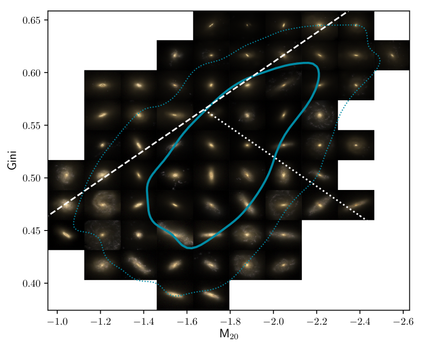
Figure 3: Mock gri-SDSS colour composite images of galaxies in the Ref-100 sample arranged according to their $G$ and M₂₀ values. Solid (dotted) contours represent the region containing 68 (95) percent of objects. The straight lines are as in Figure 2. In accordance with observational trends, prevailing morphologies at the top right of the diagram are of the early type, while galaxies at the lower left are late-type. Signs of disturbed morphologies can be found above the dashed line for some galaxies.

4.1 Gini-M₂₀

Figure 2 shows the position in the $G$-M₂₀ morphological subspace occupied by the Ref-100 sample (blue contours), the Illustris sample (orange contours), the IllustrisTNG sample (red) and the GAMA sample (coloured points). The subspace is divided into three sectors where, according to (Lotz et al., 2008b), galaxies in the Extended Groth Strip at $0.2<z<1.2$ present the following distinct morphologies:

Mergers:

$\textnormal{G}>-0.14\textnormal{M}_{20}+0.33$,

E/S0/Sa:

$\textnormal{G}\leq-0.14\textnormal{M}_{20}+0.33$ and $\textnormal{G}>0.14\textnormal{M}_{20}+0.80$,

Sb–Irr:

$\textnormal{G}\leq-0.14\textnormal{M}_{20}+0.33$ and $\textnormal{G}\leq 0.14\textnormal{M}_{20}+0.80$.

Galaxies in the gama sample are colour coded according to the T-Type assigned to them by the machine learning algorithm of Domínguez Sánchez et al. (2018). It is clear that galaxies with negative T-Type (corresponding to early-type galaxies) and those with with positive T-Types (corresponding to late-type galaxies) prefer different locations in the $G$-M₂₀ plane and that their positions generally agree well with those determined by Lotz et al. (2008b) for their respective morphological type, with some intermixing.

It can also be appreciated in Fig. 2 that the location occupied by galaxies in the Ref-100 (blue contours) coincides to a large extent with that of the gama sample. This constitutes strong evidence that the morphologies of eagle galaxies are a close match to those of real galaxies, at least at low redshift. However, some discrepancies do exist. Mainly, the distribution of gama galaxies appears to be skewed towards higher $G$ and more negative M₂₀ values, as compared to Ref-100 galaxies. This results in a larger proportion of real galaxies in the E/S0/Sa sector of the morphological space. Some of this discrepancy can be attributed to the higher median stellar mass of gama galaxies, as discussed in sections 2.3.

The discrepancies are much more pronounced for Illustris, for which the whole distribution is skewed towards lower $G$ and more positive M₂₀ values, forming an extended tail up to $M_{20}\simeq-0.5$ where almost no observational counterparts can be found. These discrepancies are more notable when considering that all three compared samples are very similar in stellar mass.

Recently, Rodriguez-Gomez et al. (2019) studied the optical non-parametric morphologies of galaxies in IllustrisTNG, they found that the updated Illustris model produces galaxies with morphologies much closer to observations. Indeed, we find that the locus of their $G$-M₂₀ distribution is close to what we find for Ref-100. It is interesting that both simulations, run with different physical models appear to result in very similar morphologies. As a matter of fact, there is a better agreement in the distribution of $G$ and M₂₀ between Ref-100 and IllustrisTNG than between any of the simulations and the gama galaxies. A possible explanation for this is that in simulations, the stellar component is represented by particles tracing the stellar density distribution, and as such, particle noise gives a granular appearance to the images even when a significant smoothing is applied. This could explain the shift towards higher M₂₀ values in the simulations, compared to gama. Also, the gravitational softening adopted in the simulations affects the distribution of matter at the nucleus of galaxies, resulting in an artificial flattening of the central surface brightness that could skew $G$ values lower.

Figure 3 shows gri-composite images of representative Ref-100 galaxies at different points in the $G$-M₂₀ plane. To construct the figure we bin galaxies by their $G$-M₂₀ values and display the image of the galaxy closest to the mean value of the bin. Visual inspection reveals that giant ellipticals and Sa type morphologies dominate the upper right sector of the figure. While galaxies with more prominent spiral arms (Sb–Sc types) are more frequent in the lowermost sector. Some small and roundish systems can also be found in this sector, especially close to the central part of the diagram ($G$ $\sim 0.52$, M${}_{20}\sim-1.75$).

Some of the galaxies found above the demarcation line separating mergers from normal galaxies show signs of disturbance. However, a majority appears to be normal, with a morphology not much different to that of galaxies located below the line. Previously, Bignone et al. (2017) found that Illustris galaxies in this region of the $G$-M₂₀ space could be associated to recent and ongoing mergers, with some contamination from normal galaxies. It is possible that the demarcation line between mergers and normal galaxies be shifted in eagle or that the merger properties in the simulation differ from observations. Recently, Pearson et al. (2019) tested whether a convolutional neural network trained on SDSS data could be used to identify mergers in eagle. They found that the network performed significantly worst when applied to the simulation, possible indicating differences between the visually selected observed mergers and the mergers selected in the simulation.

4.1.1 Bulge statistic

Similarly to Snyder et al. (2015b), we define a quantity which is a measure of the optical bulge strength. Specifically, $F$ is defined as five times the point-line distance from the galaxy’s morphology point to the Lotz et al. (2008a) early/late type separation line. We also set the sign of $F$ so that positive (negative) values indicate bulge-dominated (disc-dominated) galaxies.

$$|F| =-0.693*M_{20}+4.95\,\textnormal{G}-3.96,$$ (7)

$$F(G,M_{20}) =\begin{cases}|F|\qquad G\geq 0.14*M_{20}+0.80,\\ -|F|\qquad G<0.14*M_{20}+0.80.\\ \end{cases}$$

Figure 4: T-type versus $F$ for galaxies in the gama sample where T-types were assigned by a deep convolutional neural network trained in visually classified galaxies (Domínguez Sánchez et al., 2018). Red points represent negative T-type (bulge-dominated) objects, while blue points represent positive T-type (disc-dominated) objects. The bulge strength indicator $F$ is mostly successful at separating the early and late types as shown by the normalized $F$ distributions at the top panel. The top right and bottom left corners of the figure contain the minority of objects for which the T-type and $F$ classification are in conflict (see text for more details).

Figure 4 shows the distribution of $F$ for gama galaxies, differentiating positive and negative T-Type populations. We can appreciate that the $F=0$ separation line is located very close to the point where the number of early type galaxies starts to dominate. We can also ascertain the level of contamination that using only $F$ as an assessment of morphological type would entail. A total of 94 galaxies (28 per cent of T-Type $>$ 0 galaxies) are classified as late-type according to their T-Type, but as bulge-dominated according to $F$. On visual inspection, a large number of these systems appear to be edge-on discs or low-contrast discs which the machine learning algorithm is able to classify, but that represent a challenge for simple heuristics derived from non-parametric statistics.

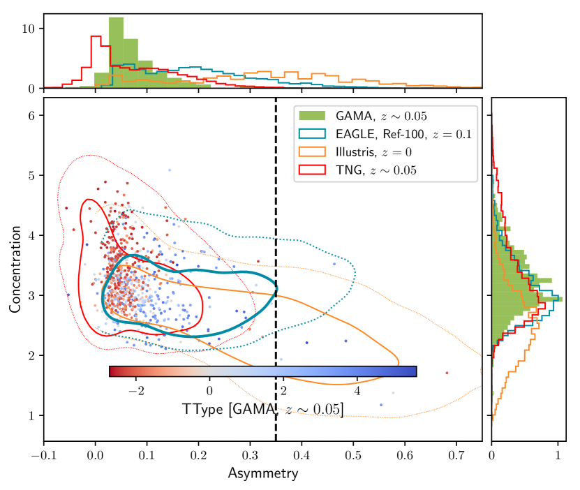
Figure 5: The central panel shows the $C$-$A$ diagram from galaxies in Ref-100 (blue), Illustris (orange), IllustrisTNG (red) and gama (points). The coloured Solid (dotted) lines enclose regions containing 68 (95) percent of galaxies in each respective sample. The gama galaxies are coloured according to their T-Types. The black dashed line at $A$=0.35 separates normal from merging or highly disturbed galaxies. The distribution of $C$s for Ref-100 and IllustrisTNG are in good agreement with that of gama, while Illustris exhibits a tail towards lower lower $C$s. All simulations have a tail towards higher asymmetries in excess of what is observed, the effect is more notorious for Illustris. $A$ for IllustrisTNG galaxies appear systematically shifted towards lower values, this is due to slight changes in the algorithm used to compute the statistic, see text for details.

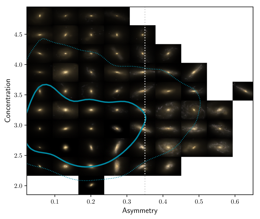
Figure 6: Mock gri-SDSS colour composite images of galaxies in the Ref-100 sample arranged according to their $C$ and $A$ values. Solid (dotted) contours represent the region containing 68 (95) percent of objects. The straight line is as in Figure 5. In accordance with observational trends, prevailing morphologies at the top left of the diagram are of the early type, while galaxies at the lower right are late-type.

The other source of conflict comes from galaxies classified as early types by their T-Type, but as disc-dominated by $F$. There are 119 cases of this (29 % of T-Type $<$ 0 galaxies). Their location in Fig. 4 indicates that they belong to the same grouping as $F>0$ galaxies, indeed visual inspection reveals an abundant number of S0 type galaxies. Domínguez Sánchez et al. (2018) discuss the difficulty of their algorithm in differentiating between pure ellipticals and S0s, with the elliptical classification being preferred due to the larger number of training examples. This suggests that a T-Type closer to zero would actually be a better match to the morphology of these conflicting galaxies. This will also result in a tightening of the correlation between T-Type and $F$ that appears in Fig. 4.

These results confirm the robustness of the demarcation line to separate late and early-type morphologies. We find there is no clear alternative demarcation line in $F$ to that of Lotz et al. (2008a) that better separates positive and negative T-Types.

4.2 Concentration-Asymmetry

Figure 5 shows the position in the $C$-$A$ morphological subspace occupied by the Ref-100 sample (blue contours), the Illustris sample (orange contours), the IllustrisTNG sample (red) and the gama sample (coloured points). The subspace is divided into two sectors by a vertical line at $A=0.35$ which serves to separate mergers from normal galaxies (Lotz et al., 2008b). The observational gama sample exhibit the expected trends between T-type morphology and non-parametric statistics with giant ellipticals presenting high $C$ and low $A$ and late-type disks (Sc–Sd) presenting low $C$ and high $A$. Intermediate cases appear mixed at approximately $C\sim 3$, $A\sim 0.07$.

It is clear from Fig. 5 that while the $C$ distribution of the Ref-100 and gama samples are a close match, that is not the case of the $A$ distribution. Simulated galaxies exhibit a large tail towards higher asymmetries that do not match observations. Similar results were obtained for the Illustris simulation (Bignone et al., 2017). Simulated asymmetries have a bimodal distribution with a low $A$ population that approximately follows observational trends and another, highly asymmetrical population, for which there are no observational counterparts.

For IllustrisTNG we find a similar behaviour as Ref-100, but with $A$ shifted towards lower values. This is largely a consequence of the different implementation of the computation of asymmetries between the simulated samples, as described in Section 3.3.4. IllustrisTNG also shows a larger tail towards high $C$ galaxies, compared to Ref-100. These galaxies also correspond to systems with higher $G$ coefficients and M₂₀, compared to Ref-100 and primarily affects massive galaxies.

Figure 6 shows colour-composite of Ref-100 galaxies arranged by their position in the $C$-$A$ plane. Normal spiral galaxies are mostly found with asymmetries well beyond 0.35, which normally would indicate disturbed morphologies. It is clear that asymmetry is being driven by the light distribution of young star-forming regions in the simulated galaxies. In fact, very young star formation regions are conspicuous in every image where they are present, because of their scattered and point-like appearance. This is true even for galaxies with a bulge-dominated morphology. It is therefore likely that this is an effect of the way the simulated data is being translated into the mock images for this young stellar populations, specifically the way photon sources are spatially distributed (Torrey et al., 2015). A possible mitigation strategy could be to assign young stellar particles an increased smoothing length in the mock image generation procedure (Trayford et al., 2017).

4.3 Spatial resolution Effects

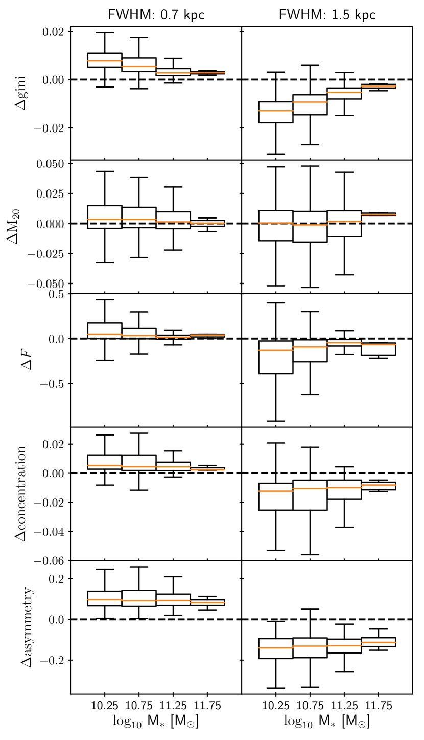
Figure 7: Boxplots describing the median relative changes in morphological values obtained as a consequence of varying the spatial resolution of images by using different FWHM values in the procedure described in Section 3.1.3. Changes in the statistics are measured from those obtained using a FWHM=1.0 kpc. $G$ values are systematically reduced with decreasing resolution, but the effect is larger for decreasing stellar mass. $F$ is the most robust statistic in terms of changes in the spatial resolution, while $A$ is the most affected overall.

Non-parametric morphologies can be affected by several factors. Among them, limited image spatial resolution. Understanding these effects is important, particularly when contrasting local against high-redshift galaxies, where the signal-to-noise ratio and the spatial resolution are expected to be worse. Also, large-scale galaxy surveys (such as SDSS and LSST) which are ideally suited for statistical studies because of their large sample sizes and the comprehensive sets of measured quantities, likely suffer from limited resolution.

Previously, Lotz et al. (2004) studied the effect of decreasing spatial resolution on the values of $G$, M₂₀, $C$, and $A$. They found that $C$ and M₂₀ were reliable up to resolution scales of 500 pc pixel^-1, while $G$ and $A$ where stable down to 1000 pc pixel^-1. However, their results were restricted to a small sample of 8 galaxies of various morphological type. Here, we have the advantage of a much larger number of simulated galaxies that also happen to cover a wide range of morphologies, stellar masses, star formation rates (SFRs) and orientations. Therefore, we can give a more statistically reliable assessment of the effect of spatial resolution on non-parametric morphologies.

To study the effect of decreasing resolution we vary the value of the FWHM used to approximate the seeing in the procedure described in section 3.1.3. We consider FWHM values equal to 0.7 kpc, 1.0 kpc and 1.5 kpc. Results for the intermediate FWHM $=1.0$ kpc are shown thought this work and constitutes our value of reference. At 0.7 kpc, the first value represents an instrument with the same spatial resolution as in the Ref-100 simulation. Also, for $z\sim 0.05$ galaxies a FWHM = 0.7 kpc produces images with the expected spatial resolution of the upcoming LSST, which will have a mean seeing of 0.7 arcsec. Finally, the last FWHM value more closely represent the seeing present in SDSS.

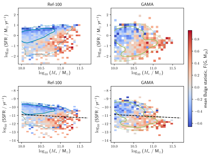
Figure 8: Top panels: SFR versus stellar mass for galaxies in the Ref-100 (left) and gama samples (right). with colours proportional to the mean bulge strength $F$ in each 2D bin. Solid (dotted) lines enclose regions that contain 68 (95) percent of objects. Bottom panels: the same as the top panels but for SSFR versus stellar mass. The dashed line separates active from passive galaxies according to the criteria of Omand et al. (2014). Ref-100 presents very similar trends in stellar mass, star formation and optical morphology compared to gama, the most notable difference being an excess of active galaxies in the upper stellar mass end of the relation for Ref-100, for which there are no observation counterparts.

We divided the Ref-100 galaxy sample into four subsamples according to stellar mass. In Fig 7 we show boxplots describing the median relative changes in morphological values obtained as a consequence of using different FWHM values for each subsample. Changes are measured from results obtained with FWHM $=1.0$ kpc according to:

$$\Delta_{X_{i}}=\frac{X_{i}-X_{1.0\,\textnormal{kpc}}}{\left|X_{1.0\,\textnormal{kpc}}\right|},$$ (8)

where $X$ represents $G$, $M_{20}$, $F$, $C$ or $A$, while the suffix $i$ stands for one of the tested FWHM values: 0.7 and 1.5 kpc.

We find that $G$ is systematically reduced with decreasing spatial resolution. Also, the effect is larger for lower mass galaxies. For FWHM=0.7 (1.5) kpc and stellar masses $\sim 10^{10.25}$ M_⊙, the median change in $G$ with respect to the reference values is $\sim 0.8$ ($\sim 1.5$) per cent higher (lower). In contrast, M₂₀ is less effected, with median shifts less than 0.8 per cent for both FWHM values, across all mass bins. $F$ is also systematically reduced with decreasing spatial resolution, this is most noticeable for FWHM=1.5 kpc, where median shifts in $F$ are $\sim 10$ per cent towards lower values. Also, there is a large scatter in $\Delta_{F_{i}}$, specially in the two lower mass bins. Results indicate that G-M₂₀ values of larger mass galaxies are comparably more robust. This can also be appreciated in Figure 2 where both simulated and observed galaxies with $F<0$ appear to move away from the Lotz et al. (2008b) line in the direction predicted by the resolution effect. $F>0$ galaxies on the other hand, have a distribution parallel to the Lotz et al. (2008b) line. This behaviour can be easily explained by the smoother light distribution of early-type galaxies that is largely unaffected by additional smoothing by the seeing. These spatial resolution effects could also explain why the demarcation line was found to be slightly different between the Lotz et al. (2004) and Lotz et al. (2008b) studies, since the latter study was based on a closer sample of galaxies with the consequential higher spatial resolution.

$C$ only shows a small systematic effect of less than 2 per cent even for the 1.5 kpc worst case scenario, and a small dependence on stellar mass. While the quantity most affected by spatial resolution is $A$, which exhibits values 14 per cent lower for FWHM=1.5 kpc. However, simulated asymmetries are considerably larger than observed ones, as previously discuss, so it is likely that this effect is a product of the simulated nature of the images and not directly applicable to observational results.

4.4 Dependence on star formation

Measurements of Sérsic index and compactness are found to correlate with galaxy quiescence (e.g. Wuyts et al., 2011; Bell et al., 2012) indicating that galaxy morphology and star formation are closely related.

In Figure 8 we plot the mean values of the bulge statistic $F$ in bins of (SFR, M_∗) and (SSFR, M_∗). To each of these mean $F$ values we assign colours from blue (disc-dominated) to red (bulge-dominated). We also plot contours containing 68 percent (solid lines) and 95 percent (dotted line) of the galaxies in each sample. The star formation rate is extracted directly from the simulation in the case of Ref-100 and from H$\alpha$ luminosity measurements for gama galaxies (Gunawardhana et al., 2013).

We find that Ref-100 galaxies roughly recover the main sequence of star-forming galaxies (e.g. Whitaker et al., 2012). Although, results by Furlong et al. (2015) showed that the Ref-100 simulation presented SSFRs $\sim 0.2$ dex lower compared to other observational data sets (Gilbank et al., 2010; Bauer et al., 2013). Despite these possible offsets in the normalization, we find that in general terms lower SFR galaxies of the same stellar mass have, on average, a more bulge-dominated morphology. There is a good agreement between the SFR-M_∗-F relation of simulated and observed samples.

We also find that the bulge-dominated morphologies are mostly found for stellar masses $>10^{10.5}$ M_⊙ and with SSFRs consistent with quenched star formations, as indicated by their position below the line separating active and passive galaxies according to Omand et al. (2014). However, some bulge-dominated systems can still be found among star-forming galaxies (Rosito et al., 2018b). Also passive galaxies can have disc morphologies, but these tend to be relegated to lower mass systems.

There is a population of star-forming and high-mass galaxies in Ref-100 for which there is no equivalent among the gama sample. This suggests that the quenching mechanisms in the simulation are not efficient enough in these particular cases. This is in line with results by Furlong et al. (2015) who found $\sim 15$ per cent too few passive galaxies between $10^{10.5}$ and $10^{11.5}$ M_⊙ in Ref-100, compared to observations. We find that the Morphologies of these galaxies are mostly late-type, but early-types start to dominate at lower SFRs.

4.5 Dependence on size

The bottom panels of Figure 9 show the bulge statistic $F$ as a function of galaxy size. The galaxy size is parametrized by the semimajor axis of an ellipse containing half of the total luminosity of the galaxy. Upper panels show the size distribution of galaxies discriminating between bulge-dominated ($F\geq 0$) and disc-dominated ($F<0$) systems. Both Ref-100 and gama samples present similar flat distributions, with the observational data presenting a slightly higher degree of correlation between disc strength and galaxy size. Meaning that gama galaxies with more disc-dominated morphologies present slightly higher median sizes.

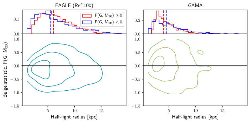
Figure 9: Bulge strength statistic $F$ versus galaxy size parametrized by the semimajor axis of an ellipse containing half of the total flux. The panel on the left shows galaxies in Ref-100, while the panel on the right shows galaxies from gama. The contours indicate the overall distribution of galaxies, while the histograms at the top panels indicate the normalized distribution of galaxy sizes discriminating between early ($F>0$) and late ($F<0$) optical morphologies. The coloured dashed lines in the histograms represent the median half-light radius of each subsample. There is an approximate agreement between Ref-100 and gama in terms of the optical morphology dependence on size. Although the correlation is slightly stronger for gama galaxies, meaning that gama galaxies with more disc-dominated morphologies present slightly higher median sizes.

Furlong et al. (2017) studied the evolution of galaxy sizes in the eagle simulations. They found that the dependence of the sizes of simulated galaxies on stellar mass and star formation is close to that of observed galaxies. They also found that active galaxies are typically larger than their passive counterparts at a given stellar mass. This is in general agreement with the results we find for the gama sample.

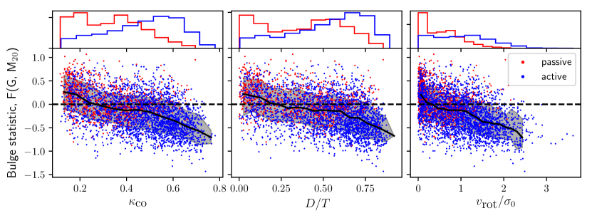
Figure 10: The bottom panels show the bulge strength statistic $F$ versus $\kappa_{\textnormal{co}}$ (left), D/T (centre) and $v_{\textnormal{rot}}/\sigma$ (right) for Ref-100 galaxies. The solid lines show the binned median and 1$\sigma$ (16th-84th) percentile scatter of the dependent variables. Overall, the optical morphology shows a strong anti-correlation with the kinematic metrics of morphology. The bottom panels show the normalized distribution of each kinematic metric for active (blue) and passive (red) galaxies.

Similar comparisons between morphology and galaxy size are discussed in Rodriguez-Gomez et al. (2019) for the cases of Illustris and IllustrisTNG. They found that, while late-type Illustris galaxies are indeed larger than their early-type counterparts, the inverse is true for IllustrisTNG galaxies. Meaning that there is tension in the size-morphology relation between observed and IllustrisTNG galaxies.

It should also be pointed out that Illustris galaxies are about two times larger than observations at $z=0$ and that IllustrisTNG galaxies show an overall better agreement with observations in terms of sizes and observational qualitative trends of size with stellar mass, star formation rate and redshift (Genel et al., 2017). In general terms, this means that both Illustris simulations are in tension with observations, albeit for different reasons. Ref-100 galaxies, however, show no significant tension with the GAMA results as shown in Furlong et al. (2017) and by the present results.

4.6 Dependence on rotation

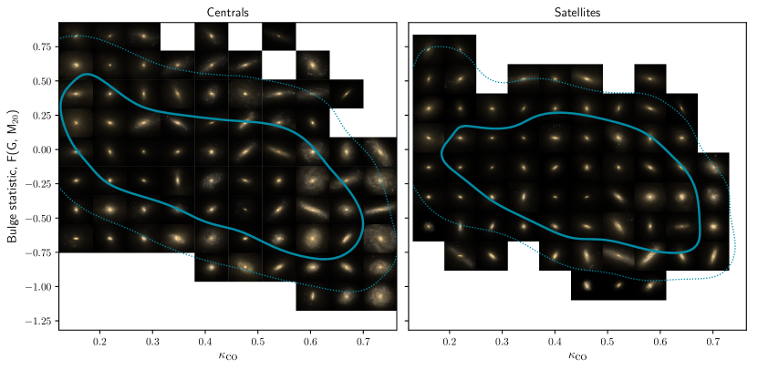
Figure 11: Mock gri-SDSS colour composite images of galaxies in the Ref-100 sample arranged according to their $F$ and $\kappa_{\textnormal{co}}$ values. The left (right) panel contains central (satellite) galaxies. Solid (dotted) contours represent the region containing 68 (95) percent of objects. The Figure illustrates the general trend of bulge-dominated galaxies appearing on the top left of the diagram while disc-dominated appear mostly on the lower right corner. Central galaxies with $\kappa_{\textnormal{co}}\sim 0.5$ but high $F$ values exhibit a disky appearance but with a prominent bulge. Satellites have a distinct appearance from their central counterpart at equal ($F$, $\kappa_{\textnormal{co}}$) values. In general, they appear smoother and with less prominent discs.

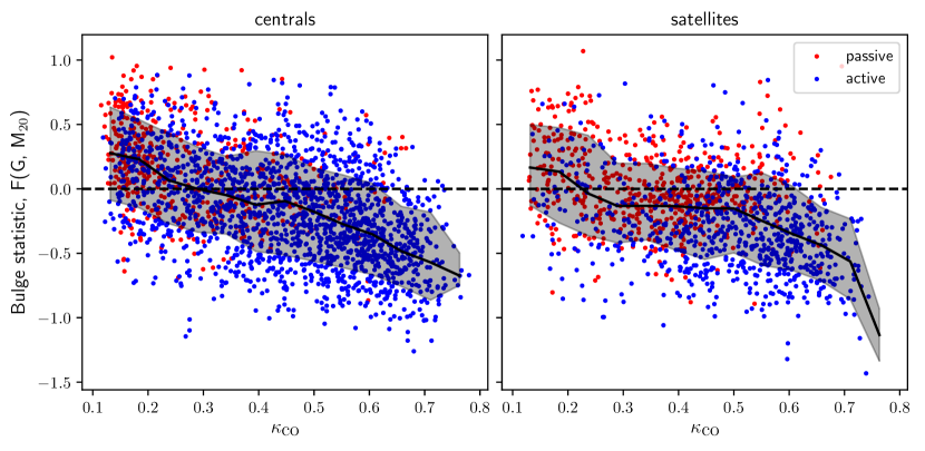
Figure 12: As the first panel of Figure 10 but discriminating between central (left panel) and satellite (right panel) galaxies. Satellites show less correlation between $F$ and $\kappa_{\textnormal{co}}$ than centrals, this is mainly due to a population of lower stellar mass, quenched satellites that occupy the central location in the relation. These galaxies present a similar bulge-dominated appearance independently of their rotational support.

There is a clear correlation between the internal kinematics of galaxies and their morphological appearance. In general terms, disc galaxies have been shown to be supported by rotation, while spheroidal systems, such as ellipticals are supported by dispersion. However, recent surveys have revealed that the connection between internal kinematics and morphology is not straightforward. In particular, the stellar angular momentum of early type galaxies have been found to span a range of values from slow to fast rotators, while a majority of S0 galaxies have been found to be fast rotators (Emsellem et al., 2011), suggesting that early and lenticular types belong to the same class but differentiate on their degree of rotational support. This indicates that kinematic diagnostics might give a more fundamental and physically motivated classification scheme (e.g. Emsellem et al., 2007; Krajnović et al., 2008; Cappellari et al., 2011). Strong correlations between optical morphology and rotation have also been found for late-type galaxies, suggesting the existence of a fundamental relation between angular momentum, stellar mass and optical morphology across all Hubble types (e.g Romanowsky & Fall, 2012; Obreschkow & Glazebrook, 2014; Cortese et al., 2016)

Since stellar and gas kinematics are easily extracted from simulations, kinematic diagnostics have long been used as a proxy for optical morphology. These diagnostics generally summarize galaxy kinematics in a single parameter such as the $\kappa_{\textnormal{rot}}$ parameter (Sales et al., 2010), the bulge-to-total ratio (B/T) or the disc-to-total ratio (D/T) (e.g. Scannapieco et al., 2008). In the case of eagle, variations of these metrics have been studied by Correa et al. (2017); Correa et al. (2019), Clauwens et al. (2018), Trayford et al. (2019) and Tissera et al. (2019).

In Figure 10 we show the optically derived $F$ bulge strength statistics as a function of three kinematic metrics: $D/T$, the fraction of kinetic energy that is invested in co-rotation ($\kappa_{\textnormal{{co}}}$, Correa et al., 2017) and the ratio of rotation and dispersion velocities ($v_{\textnormal{rot}}/{\sigma}$). All three quantities are extracted from the eagle public database and are based on the corresponding definitions found in Thob et al. (2019). We find that $F$ anti-correlates with all three kinematic diagnostics to a similar extent, a Spearman’s rank test gives correlation coefficients of -0.46, -0.46 and -0.43 between $F$ and $\kappa_{\textnormal{{co}}}$, $D/T$ or $v_{\textnormal{rot}}/{\sigma}$, respectively. The scatter in $F$ is $~{}0.7$ dex for all three kinematic metrics. This shows that the optical morphologies of the simulated galaxies correlate with the degree of rotational support to a large extent. The similar correlation coefficients found are in line with results by Thob et al. (2019) that show that these commonly used kinematic metrics are strongly correlated in eagle and can in general be used interchangeably.

Also in Figure 10 we distinguish between active (blue points) and passive galaxies (red points) using the same criteria as in Section 4.4. It is apparent that $\kappa_{\textnormal{co}}$ is the most successful among the kinematic metrics in separating between star-forming and quenched galaxies as can be appreciated from the normalized histograms in the top panels, indeed Correa et al. (2017) showed that simple threshold at $\kappa_{\textnormal{co}}=0.4$ serves to separate galaxies in the red sequence from those in the blue cloud. We notice that such a value of $\kappa_{\textnormal{co}}$ roughly corresponds to the transition between optically bulge dominated ($F>0$) and disc dominated ($F<0$) galaxies. This serves to confirm in a quantitative way that that choice of $\kappa_{\textnormal{co}}$ threshold is also successful at separating galaxies that look disky from those that look elliptical.

However, we also notice that using a threshold in $F$ instead of $\kappa_{\textnormal{co}}$ to classify galaxies selects in principle, different galaxy subsets. In particular, there is a group of active galaxies around $\kappa_{\textnormal{co}}\sim 0.5$ that presents positive $F$. These galaxies would be classified as disc-dominated according to their kinematics, but as bulge-dominated according to their light distribution. In Figure 11 we investigate the visual appearance of galaxies based on their location in the $F$ versus $\kappa_{\textnormal{co}}$ space. We confirm the general trend that early type and late type galaxies are located respectively in the top left and bottom right of the diagram. We also notice that the mentioned subset of galaxies with contradicting kinematic and optical morphologies are mostly central galaxies with active star-forming regions and tend to have more of a disky morphology. However, they differ from the pure spirals in that their disc and arms appear less prominent, which would explain why they are being assigned positive $F$ values. These galaxies could correspond to disc+bulge galaxies explored by Clauwens et al. (2018).

The right panel of Figure 11 show galaxy images for satellite galaxies. Compared to the central galaxies on the left, they present a somewhat different appearance. For equal ($F$, $\kappa_{\textnormal{co}}$) satellites are more compact, present less prominent discs and generally a smoother appearance, indicating differences in their evolution. This can be expected if for example. environmental processes result in additional quenching mechanisms (Kauffmann et al., 2004) in satellites. Figure 12 further explores the difference between central and satellite galaxies in the correlation between $F$ and $\kappa_{\textnormal{co}}$. We find that optical and kinematic morphology indicators are more correlated in the case of centrals, indeed a Spearman’s rank test gives correlation coefficients of -0.5 and -0.38 between $F$ and $\kappa_{\textnormal{{co}}}$ for central and satellite galaxies, respectively. For satellites it can be appreciated that there is a flattening in the relation at $\kappa_{\textnormal{co}}\sim 0.3$ where there is an abundance of quenched galaxies. Inspection of Figure 11 reveals that these are mostly smallish, lower mass systems that likely experienced environmental quenching without having gone through a kinematic transformation. This result is in agreement with Cortese et al. (2019) who found that satellites undergo little structural change before and during the quenching phase.

In contrast, satellites with low $\kappa_{\textnormal{{co}}}$ and high $F$ values appear clustered apart and their visual appearance is more similar to their central counterparts. This indicates that for these higher stellar mass systems, environmental quenching is not as important and that their morphological evolution is more akin to that of central galaxies.

5 Summary and discussion

We have studied the optical morphologies of $z=0.1$, $M_{*}>10^{10}$ M_⊙ galaxies in the eagle Ref-100 simulation using non-parametric statistics (Gini, M₂₀, Concentration and Asymmetry) derived from the g-band light distribution in mock images obtained from radiative transfer techniques including the effect of dust and post-processed to mimic images in the SDSS survey. We have compared the Ref-100 morphologies with those of galaxies from the gama survey and from other numerical simulation, Illustris and IllustrisTNG. Morphologies of simulated and observed images were obtained in a very similar manner using the same statmorph code (Rodriguez-Gomez et al., 2019)

Our conclusions can be summarized as follow:

(i) Optical eagle morphologies indicated by their distribution of $G$ and M₂₀ statistics agree well with those derived from SDSS images of gama galaxies selected to have $z\sim 0.05$ and $M_{*}>10^{10}$ M_⊙, closely matching the simulated sample selection.

(ii) The ($G$, M₂₀) morphologies of gama galaxies correlate well with their T-Type morphologies obtained using a deep neural network trained on visual classification (Domínguez Sánchez et al., 2018). Moreover, we find that the demarcation line separating bulge from disc dominated morphologies according to Lotz et al. (2008b) performs that task very well for our observational and simulated sample and therefore is a robust basis for the definition of the bulge strength statistics $F$ (Snyder et al., 2015b).

(iii) Simulated galaxies from the Illustris simulation (Snyder et al., 2015b) present some discrepancies with those in eagle and gama, particularly for a subset of galaxies at low $G$ and high M₂₀ values for which there are no counterparts in the mentioned samples. In contrast, simulated morphologies of IllustrisTNG galaxies Rodriguez-Gomez et al. (2019) agree remarkably well with those in our Ref100 and gama samples. This indicates that there is a convergence between the simulations in terms of these morphological statistics, possible due to the fact that both simulations reproduce to a large extent at $z\sim 0$ basic galaxy properties such as stellar mass, size and star formation rate. Given that a significant portion of galaxy morphology is determined by these factors, this is perhaps not that surprising. It is still remarkable, that we can make such a straightforward and direct quantitative comparison between the optical morphologies of these various simulations and also observations.

(iv) Although there are disturbed and interacting simulated galaxies present in the ($G$, M₂₀) region commonly assigned to merger and irregular galaxies (Lotz et al., 2008b) we find that there is significant contamination from normal galaxies. Recently, Pearson et al. (2019) used a convolutional neural network to identify mergers in SDSS and in eagle mock images, they found that the network lost significant performance when trained or applied to eagle images as compared to SDSS images. This indicates that the visual appearance of normal and merging Ref-100 galaxies might present discrepancies when compared to observations.

(v) Further discrepancies are found for the $A$ statistic. Normal Ref100 spiral galaxies have significantly larger asymmetries that their gama counterparts and similar behaviour is observed for Illustris and IllustrisTNG galaxies. This is an indication that despite the general good agreement between observed and simulated morphologies, simulations still present differences in their more detailed appearance. A likely explanation for this is that the distribution of photon sources from young stellar population in the image generation procedure is resulting in artificially high asymmetries. We suggest that a possible mitigation strategy could be to assign young stellar particles an increased smoothing length in the mock image generation procedure (Trayford et al., 2017). Recently, Dickinson et al. (2018) presented the visual morphological classification of Illustris galaxies derived from Galaxy Zoo citizen scientists. They identified significant differences between Illustris and real SDSS images. Specifically, a much larger fraction of simulated galaxies were classified as presenting visible substructure,relative to their SDSS counterparts. As per (iii), both eagle and IllustrisTNG appear to better match observations compared to the original Illustris, future studies of this kind could determine if these improvements are enough to also result in a better match with respect to human visual classification. In that direction we also point out that a similar neural network to the one used to classify T-type morphologies in (ii) has recently been used to classify IllustrisTNG galaxies (Huertas-Company et al., 2019). The authors found that the neural network, trained on SDSS visual morphologies was successful at identifying simulated galaxies in four classes (E, S0/a, Sab and Scd). In summary, while very detailed morphologies might need further improvements, it appears that simulations are successful in reproducing general visual morphologies.

(vi) The large sample size of simulated galaxies spanning a large range of stellar masses, sizes and morphologies allows us to study in better statistical detail the effect that spatial resolutions has on the non-parametric morphologies. This is particularly important in light of future surveys, such as LSST where this kind of automatic morphological classification is expected to be implemented on a very large scale (Collaboration et al., 2009). We vary the value of the FWHM used to approximate the seeing between 1.0 kpc (the reference value), 0.7 kpc (the value expected for LSST), and 1.5 kpc (a value that more closely match SDSS imaging). We find that $G$ is systematically lower for decreasing resolution and that such effect depends on stellar mass, with the lower mass galaxies presenting the largest effect. Similar effects are also found for $F$. $A$ appears to be the statistic most affected by spatial resolution, with significantly lower $A$ values with decreasing resolution. Although, no apparent dependence on stellar mass was found, this is in contrast to what was found by Bignone et al. (2017) in the case of Illustris, for which lower mass galaxies were systematically more asymmetric.

(vii) Ref100 galaxies present the expected trends between optical morphology (summarized by the bulge strength $F$), stellar mass and star formation rate, where at equal stellar mass, galaxies with lower SFR have, on average, a more bulge-dominated morphology. The general trends found for Ref100 and gama galaxies are very similar, with some discrepancies. Specifically, there is an excess of active Ref-100 galaxies at M_∗ $>10^{11}$ M_⊙ for which there are no observational counterparts in gama, despite the similar stellar mass distribution of the samples. This is consistent with previous results by Furlong et al. (2015) who found $\sim 15$ percent fewer Ref-100 passive galaxies in the stellar mass range $10^{10.5}-10^{11.5}$. We find that these galaxies present a mix of bulge-dominated and disc-dominated morphologies.

(viii) There is a general agreement between the size-morphology relation of galaxies in the Ref-100 and gama samples, in that they both present a similar flat trend in $F$ versus Half-light radius. Although, disc-dominated gama galaxies appear to be slightly larger than their bulge-dominated counterparts, in line with previous results by Furlong et al. (2017) who found that active galaxies are typically larger than their passive counterparts at a given stellar mass.

(ix) We find a significant correlation between the optical morphology of Ref-100 galaxies, characterized by their bulge strength $F$ and kinematic morphologies expressed by D/T, $\kappa_{\textnormal{co}}$ and $v_{\textnormal{rot}}/\sigma$. In general terms, optically bulge-dominated galaxies have lower rotational support and higher velocity dispersion.

(x) We find that a threshold value of $\kappa_{\textnormal{co}}=0.4$ (Correa et al., 2017) roughly corresponds to our $F=0$ threshold separating bulge-, from disc-dominated systems. However, we notice that the optical and kinematic criteria do not select the same galaxy populations. In particular, the optical criteria for bulge-dominated systems differs in that it also selects a number of actively star-forming central galaxies with significant rotational support and visually disky appearance. These galaxies differ from pure spirals in that their discs and arms are less prominent and they present a significant bulge component.

(xi) Central galaxies present a higher degree of anti-correlation between $F$ and $\kappa_{\textnormal{co}}$, compared to the one found for satellites. This is due to satellites presenting a significant number of low stellar mass, quenched systems with $F\sim 0.1$ values and $\kappa_{\textnormal{co}}$ between [0.3, 0.5]. This is an indication of different morphological evolution in centrals and satellites, with smaller mass satellites being more affected by environmental quenching that shuts down star formation leaving the disc initially intact. This is in line with results by Cortese et al. (2019) who found that changes in stellar kinematic properties become evident at a later stage and that satellites tend to remain rotationally dominated. Also, Trayford et al. (2016) found that lower mass Ref-100 galaxies are quenched by environmental effects once they become satellites. While, higher stellar mass, central galaxies, are quenched mainly by AGN feedback (Trayford et al., 2016; Bower et al., 2017). Higher mass central and satellite galaxies present a similar appearance in terms of both optical morphology and their degree of rotational support. It is expected that for higher mass satellites, environmental quenching is not as important and that their morphological evolution can be more similar to that of central galaxies.

Appendix A Dependence on orientation

In the main body of the paper we present the results corresponding to a random orientation with respect to the galaxy (but fixed to the $xy$ plane of the simulation box). Here we compare those results with two other extreme viewing angles: edge- and face-on views. Figure 13 shows the variation in the distributions of $G$, M₂₀, $C$ and $A$ caused by considering the different viewing angles. Compared to their randomly oriented counterparts, we find that edge-on views result in higher median M₂₀ and $G$ values (4% and 1.3%, respectively). However, the largest changes are found for the case of $A$ where edge-on (face-on) views result in a median value 14% (10%) lower (higher). Unsurprisingly, the effects of orientation are more noticeable in lower-mass, disky and star-forming galaxies.

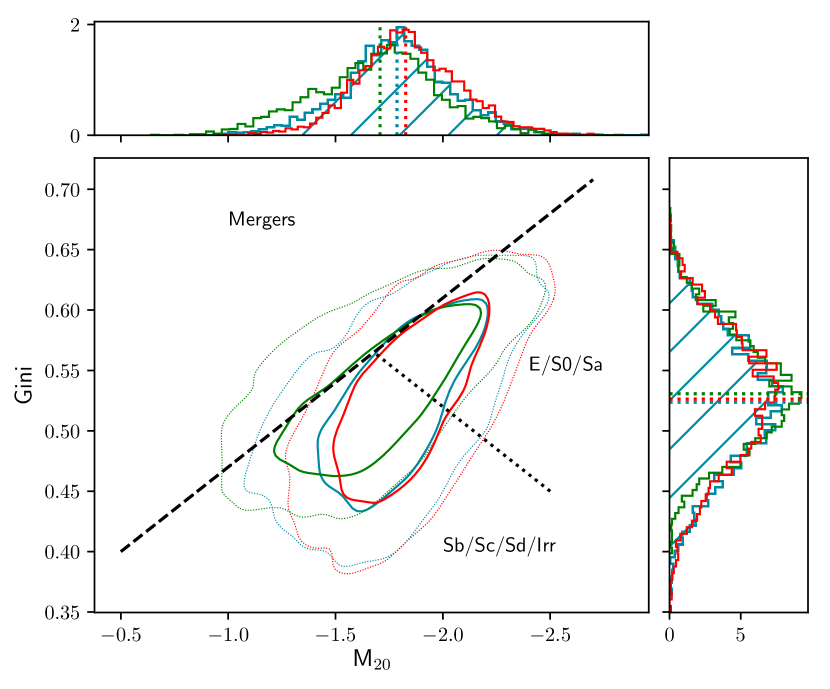
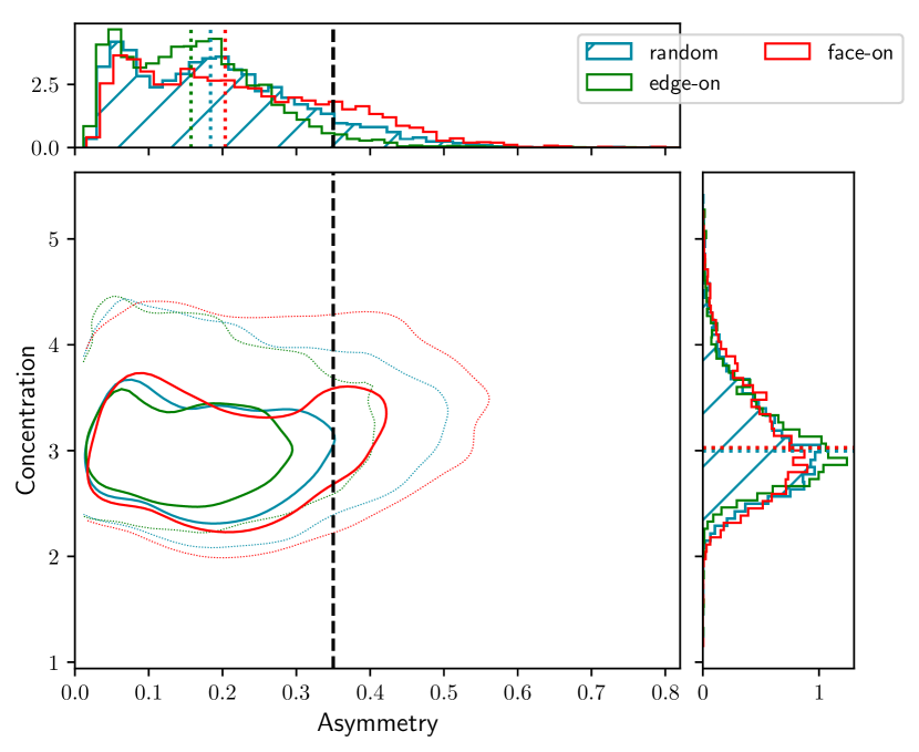
Figure 13: $G$ versus M₂₀ (panel on the left) and $C$ versus $A$ (panel on the right) for Ref-100 galaxies. We compare the results of three viewing angles: face-on, edge-on and a random orientation with respect to the galaxy (but fixed to the $xy$ plane of the simulation box). The random orientation was used thought the main body of the paper.

Appendix B Numerical convergence

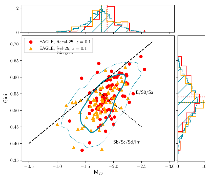
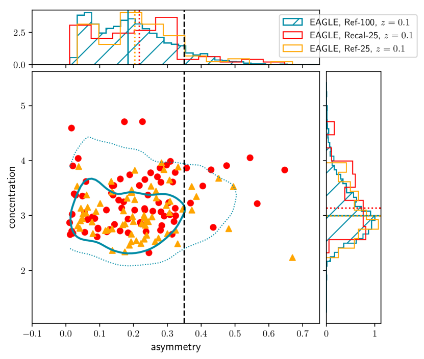
Figure 14: $G$ versus M₂₀ (panel on the left) and $C$ versus $A$ (panel on the right) for galaxies in the Recal-25 (red points and lines), Ref-25 (orange triangles and lines) and Ref-100 (cyan contours) simulations. Non-parametric statistics were computed from a face-on viewing angle.

To test numerical convergence, we compare the non-parametric morphologies of galaxies in the Ref-100 simulation with those in a simulation with resolution a factor 8 finer in mass and a factor 2 finer in length scale, Recal-25. This constitutes a test of weak convergence, as discuss in Schaye et al. (2015), given that the subgrid model of the higher resolution simulation has been recalibrated. In Figure 14 we show the distributions of $G$, M₂₀, $C$ and $A$ for galaxies in Ref-100 (cyan lines), Recal-25 (red points and lines) and Ref-25 (orange triangles and lines). Non-parametric statistics were computed from a face-on viewing angle, to eliminate the effects of orientation. We find that Recal-25 galaxies occupy a similar distribution in morphological space as its lower resolution counterparts. However, there are slight tensions.

In table 3 we show the results of two-sample Kolmogorov–Smirnoff (KS) tests comparing the distributions of morphological statistics of galaxy samples extracted from Recal-25 against the sample extracted from the Ref-100 simulation. We find that the null hypothesis that Recal-25 and Ref-100 share the same distribution of morphological parameters should be marginally rejected for the cases of M₂₀ and $C$. Galaxies in Recal-25 exhibit a median M₂₀($C$) 3.3% (3.5%) higher (lower) than galaxies in Ref-100. The other statistics considered: $G$ and $A$ have distributions that are statistically equivalent according to the KS tests.

Ref-25 has the same volume size as Recal-25, but shares resolution with Ref-100 instead, its inclusion serves to control against box-size effects. The same KS-test applied to the Ref-25 simulation indicate that the simulation share similar distributions with Ref-100 for all statistics considered, which allow us to reject effects due to the smaller volume.

The differences between Recal-25 and Ref-100 are not large enough to affect the morphological trends presented in the main body of the paper and therefore do not affect our conclusions significantly. It is also interesting to point out that the mock morphological statistic that most diverges from the observations, $A$, is not particularly affected by numerical resolution. Therefore we should look for the reasons of this discrepancy in the image generation procedures.

Table 3: Results of two-sample Kolmogorov–Smirnoff tests comparing galaxy samples extracted from Recal-25 and Ref-25 against a sample extracted from the Ref-100 simulation

	Recal-25		Ref-25
	D	p-value	D	p-value
$G$	0.13	0.12	0.13	0.18
M20	0.16	0.04	0.13	0.16
$C$	0.18	0.01	0.09	0.65
$A$	0.13	0.16	0.12	0.29

References

- Baes et al. (2011) Baes M., Verstappen J., De Looze I., Fritz J., Saftly W., Vidal Pérez E., Stalevski M., Valcke S., 2011, ApJS, 196, 22
- Baldry et al. (2004) Baldry I. K., Glazebrook K., Brinkmann J., Ivezić Ž., Lupton R. H., Nichol R. C., Szalay A. S., 2004, ApJ, 600, 681
- Baldry et al. (2012) Baldry I. K., et al., 2012, MNRAS, 421, 621
- Bauer et al. (2013) Bauer A. E., et al., 2013, MNRAS, 434, 209
- Bell et al. (2012) Bell E. F., et al., 2012, ApJ, 753, 167
- Bertin et al. (2002) Bertin E., Mellier Y., Radovich M., Missonnier G., Didelon P., Morin B., 2002, Astron. Data Anal. Softw. Syst. XI, 281, 228
- Bignone et al. (2017) Bignone L. A., Tissera P. B., Sillero E., Pedrosa S. E., Pellizza L. J., Lambas D. G., 2017, MNRAS, 465, 1106
- Blanton & Moustakas (2009) Blanton M. R., Moustakas J., 2009, ARA&A, 47, 159
- Bottrell et al. (2017) Bottrell C., Torrey P., Simard L., Ellison S. L., 2017, MNRAS, 467, 1033
- Bourne et al. (2013) Bourne N., et al., 2013, MNRAS, 436, 479
- Bower et al. (2017) Bower R. G., Schaye J., Frenk C. S., Theuns T., Schaller M., Crain R. A., McAlpine S., 2017, MNRAS, 465, 32
- Bruzual & Charlot (2003) Bruzual G., Charlot S., 2003, MNRAS, 344, 1000
- Camps & Baes (2015) Camps P., Baes M., 2015, A&C, 9, 20
- Camps et al. (2016) Camps P., Trayford J. W., Baes M., Theuns T., Schaller M., Schaye J., 2016, MNRAS, 462, 1057
- Cappellari et al. (2011) Cappellari M., et al., 2011, MNRAS, 416, 1680
- Chabrier (2003) Chabrier G., 2003, PASP, 115, 763
- Clauwens et al. (2018) Clauwens B., Schaye J., Franx M., Bower R. G., 2018, MNRAS, 478, 3994
- Collaboration et al. (2009) Collaboration L. S., et al., 2009, ArXiv E-Prints, p. arXiv:0912.0201
- Conroy et al. (2009) Conroy C., Gunn J. E., White M., 2009, ApJ, 699, 486
- Conselice (2003) Conselice C. J., 2003, ApJS, 147, 1
- Conselice (2014) Conselice C. J., 2014, ARA&A, 52, 291
- Conselice et al. (2000) Conselice C. J., Bershady M. A., Jangren A., 2000, ApJ, 529, 886
- Correa et al. (2017) Correa C. A., Schaye J., Clauwens B., Bower R. G., Crain R. A., Schaller M., Theuns T., Thob A. C. R., 2017, MNRAS, 472, L45
- Correa et al. (2019) Correa C. A., Schaye J., Trayford J. W., 2019, MNRAS, 484, 4401
- Cortese et al. (2016) Cortese L., et al., 2016, MNRAS, 463, 170
- Cortese et al. (2019) Cortese L., et al., 2019, MNRAS, 485, 2656
- Crain et al. (2015) Crain R. A., et al., 2015, MNRAS, 450, 1937
- Dalla Vecchia & Schaye (2012) Dalla Vecchia C., Schaye J., 2012, MNRAS, 426, 140
- Davis et al. (1985) Davis M., Efstathiou G., Frenk C. S., White S. D. M., 1985, ApJ, 292, 371
- Dickinson et al. (2018) Dickinson H., et al., 2018, ApJ, 853, 194
- Doi et al. (2010) Doi M., et al., 2010, AJ, 139, 1628
- Domínguez Sánchez et al. (2018) Domínguez Sánchez H., Huertas-Company M., Bernardi M., Tuccillo D., Fischer J. L., 2018, MNRAS
- Dressler (1984) Dressler A., 1984, ARA&A, 22, 185
- Driver et al. (2009) Driver S. P., et al., 2009, A&G, 50, 5.12
- Driver et al. (2011) Driver S. P., et al., 2011, MNRAS, 413, 971
- Emsellem et al. (2007) Emsellem E., et al., 2007, MNRAS, 379, 401
- Emsellem et al. (2011) Emsellem E., et al., 2011, MNRAS, 414, 888
- Freeman et al. (2013) Freeman P. E., Izbicki R., Lee A. B., Newman J. A., Conselice C. J., Koekemoer A. M., Lotz J. M., Mozena M., 2013, MNRAS, 434, 282
- Furlong et al. (2015) Furlong M., et al., 2015, MNRAS, 450, 4486
- Furlong et al. (2017) Furlong M., et al., 2017, MNRAS, 465, 722
- Genel et al. (2017) Genel S., et al., 2017, preprint, 1707, arXiv:1707.05327
- Gilbank et al. (2010) Gilbank D. G., Baldry I. K., Balogh M. L., Glazebrook K., Bower R. G., 2010, MNRAS, 405, 2594
- Gómez et al. (2003) Gómez P. L., et al., 2003, ApJ, 584, 210
- Groves et al. (2008) Groves B., Dopita M. A., Sutherland R. S., Kewley L. J., Fischera J., Leitherer C., Brandl B., van Breugel W., 2008, ApJS, 176, 438
- Gunawardhana et al. (2013) Gunawardhana M. L. P., et al., 2013, MNRAS, 433, 2764
- Huertas-Company et al. (2019) Huertas-Company M., et al., 2019, ArXiv E-Prints, p. arXiv:1903.07625
- Ilbert et al. (2010) Ilbert O., et al., 2010, ApJ, 709, 644
- Jonsson (2006) Jonsson P., 2006, MNRAS, 372, 2
- Kauffmann et al. (2003) Kauffmann G., et al., 2003, MNRAS, 341, 54
- Kauffmann et al. (2004) Kauffmann G., White S. D. M., Heckman T. M., Ménard B., Brinchmann J., Charlot S., Tremonti C., Brinkmann J., 2004, MNRAS, 353, 713
- Kormendy et al. (2010) Kormendy J., Drory N., Bender R., Cornell M. E., 2010, ApJ, 723, 54
- Krajnović et al. (2008) Krajnović D., et al., 2008, MNRAS, 390, 93
- Lagos et al. (2018) Lagos C. d. P., Schaye J., Bahé Y., Van de Sande J., Kay S. T., Barnes D., Davis T. A., Dalla Vecchia C., 2018, MNRAS, 476, 4327
- Lotz et al. (2004) Lotz J. M., Primack J., Madau P., 2004, AJ, 128, 163
- Lotz et al. (2008a) Lotz J. M., Jonsson P., Cox T. J., Primack J. R., 2008a, MNRAS, 391, 1137
- Lotz et al. (2008b) Lotz J. M., et al., 2008b, ApJ, 672, 177
- Lupton et al. (2004) Lupton R., Blanton M. R., Fekete G., Hogg D. W., O’Mullane W., Szalay A., Wherry N., 2004, PASP, 116, 133
- Marinacci et al. (2018) Marinacci F., et al., 2018, MNRAS, 480, 5113
- McAlpine et al. (2016) McAlpine S., et al., 2016, A&C, 15, 72
- Naiman et al. (2018) Naiman J. P., et al., 2018, MNRAS, 477, 1206
- Nelson et al. (2015) Nelson D., et al., 2015, Astronomy and Computing, 13, 12
- Nelson et al. (2018) Nelson D., et al., 2018, MNRAS, 475, 624
- Nelson et al. (2019) Nelson D., et al., 2019, Comput. Astrophys. Cosmol., 6, 2
- Obreschkow & Glazebrook (2014) Obreschkow D., Glazebrook K., 2014, ApJ, 784, 26
- Omand et al. (2014) Omand C. M. B., Balogh M. L., Poggianti B. M., 2014, MNRAS, 440, 843
- Pawlik et al. (2016) Pawlik M. M., Wild V., Walcher C. J., Johansson P. H., Villforth C., Rowlands K., Mendez-Abreu J., Hewlett T., 2016, MNRAS, 456, 3032
- Pearson et al. (2019) Pearson W. J., Wang L., Trayford J. W., Petrillo C. E., van der Tak F. F. S., 2019, Astron. Astrophys., 626, A49
- Pillepich et al. (2018a) Pillepich A., et al., 2018a, MNRAS, 473, 4077
- Pillepich et al. (2018b) Pillepich A., et al., 2018b, MNRAS, 475, 648
- Planck Collaboration et al. (2014) Planck Collaboration et al., 2014, A&A, 571, A16
- Robitaille (2011) Robitaille T. P., 2011, A&A, 536, A79
- Robotham et al. (2010) Robotham A., et al., 2010, PASA, 27, 76
- Rodriguez-Gomez et al. (2019) Rodriguez-Gomez V., et al., 2019, MNRAS, 483, 4140
- Romanowsky & Fall (2012) Romanowsky A. J., Fall S. M., 2012, ApJS, 203, 17
- Rosas-Guevara et al. (2015) Rosas-Guevara Y. M., et al., 2015, MNRAS, 454, 1038
- Rosito et al. (2018a) Rosito M. S., Tissera P. B., Pedrosa S. E., Rosas-Guevara Y., 2018a, ArXiv E-Prints, p. arXiv:1811.11062
- Rosito et al. (2018b) Rosito M. S., Pedrosa S. E., Tissera P. B., Avila-Reese V., Lacerna I., Bignone L. A., Ibarra-Medel H. J., Varela S., 2018b, A&A, 614, A85
- Sales et al. (2010) Sales L. V., Navarro J. F., Schaye J., Dalla Vecchia C., Springel V., Booth C. M., 2010, MNRAS, 409, 1541
- Scannapieco et al. (2008) Scannapieco C., Tissera P. B., White S. D. M., Springel V., 2008, MNRAS, 389, 1137
- Scannapieco et al. (2010) Scannapieco C., Gadotti D. A., Jonsson P., White S. D. M., 2010, MNRAS, 407
- Schaye (2004) Schaye J., 2004, ApJ, 609, 667
- Schaye & Dalla Vecchia (2008) Schaye J., Dalla Vecchia C., 2008, MNRAS, 383, 1210
- Schaye et al. (2015) Schaye J., et al., 2015, MNRAS, 446, 521
- Snyder et al. (2015a) Snyder G. F., Lotz J., Moody C., Peth M., Freeman P., Ceverino D., Primack J., Dekel A., 2015a, MNRAS, 451, 4290
- Snyder et al. (2015b) Snyder G. F., et al., 2015b, MNRAS, 454, 1886
- Springel (2005) Springel V., 2005, MNRAS, 364, 1105
- Springel et al. (2001) Springel V., White S. D. M., Tormen G., Kauffmann G., 2001, MNRAS, 328, 726
- Springel et al. (2018) Springel V., et al., 2018, MNRAS, 475, 676
- Steinacker et al. (2013) Steinacker J., Baes M., Gordon K. D., 2013, ARA&A, 51, 63
- Taylor et al. (2011) Taylor E. N., et al., 2011, MNRAS, 418, 1587
- Thob et al. (2019) Thob A. C. R., et al., 2019, MNRAS, 485, 972
- Tissera et al. (2019) Tissera P. B., Rosas-Guevara Y., Bower R. G., Crain R. A., del P Lagos C., Schaller M., Schaye J., Theuns T., 2019, MNRAS, 482, 2208
- Torrey et al. (2014) Torrey P., Vogelsberger M., Genel S., Sijacki D., Springel V., Hernquist L., 2014, MNRAS, 438, 1985
- Torrey et al. (2015) Torrey P., et al., 2015, MNRAS, 447, 2753
- Trayford et al. (2015) Trayford J. W., et al., 2015, MNRAS, 452, 2879
- Trayford et al. (2016) Trayford J. W., Theuns T., Bower R. G., Crain R. A., Lagos C. d. P., Schaller M., Schaye J., 2016, MNRAS, 460, 3925
- Trayford et al. (2017) Trayford J. W., et al., 2017, MNRAS, 470, 771
- Trayford et al. (2019) Trayford J. W., Frenk C. S., Theuns T., Schaye J., Correa C., 2019, MNRAS, 483, 744
- Vogelsberger et al. (2013) Vogelsberger M., Genel S., Sijacki D., Torrey P., Springel V., Hernquist L., 2013, MNRAS, 436, 3031
- Vogelsberger et al. (2014) Vogelsberger M., et al., 2014, Nature, 509, 177
- Weinberger et al. (2017) Weinberger R., et al., 2017, MNRAS, 465, 3291
- Whitaker et al. (2012) Whitaker K. E., van Dokkum P. G., Brammer G., Franx M., 2012, ApJ, 754, L29
- Whitney (2011) Whitney B. A., 2011, Bull. Astron. Soc. India, 39, 101
- Wiersma et al. (2009a) Wiersma R. P. C., Schaye J., Smith B. D., 2009a, MNRAS, 393, 99
- Wiersma et al. (2009b) Wiersma R. P. C., Schaye J., Theuns T., Dalla Vecchia C., Tornatore L., 2009b, MNRAS, 399
- Wuyts et al. (2011) Wuyts S., et al., 2011, ApJ, 742, 96
- Zubko et al. (2004) Zubko V., Dwek E., Arendt R. G., 2004, ApJS, 152, 211
- de Vaucouleurs (1963) de Vaucouleurs G., 1963, ApJS, 8, 31