Randomly initialized EM algorithm for two-component Gaussian mixture achieves near optimality in $O(\sqrt{n})$ iterations

Abstract

We analyze the classical EM algorithm for parameter estimation in the symmetric two-component Gaussian mixtures in $d$ dimensions. We show that, even in the absence of any separation between components, provided that the sample size satisfies $n=\Omega(d\log^{3}d)$, the randomly initialized EM algorithm converges to an estimate in at most $O(\sqrt{n})$ iterations with high probability, which is at most $O((\frac{d\log^{3}n}{n})^{1/4})$ in Euclidean distance from the true parameter and within logarithmic factors of the minimax rate of $(\frac{d}{n})^{1/4}$. Both the nonparametric statistical rate and the sublinear convergence rate are direct consequences of the zero Fisher information in the worst case. Refined pointwise guarantees beyond worst-case analysis and convergence to the MLE are also shown under mild conditions.

This improves the previous result of Balakrishnan et al [BWY17] which requires strong conditions on both the separation of the components and the quality of the initialization, and that of Daskalakis et al [DTZ17] which requires sample splitting and restarting the EM iteration.

1 Introduction

The Expectation-Maximization (EM) algorithm [DLR77] is a powerful heuristic aiming at approximating the maximal likelihood estimator (MLE) in the presence of latent variables. The general setting can be described as follows: Let $(X,Y)$ be random variables distributed according to some parametrized joint distribution with density $p_{\theta_{*}}(x,y)$. Observing $Y$ (but not the latent $X$), the goal is to estimate the true parameter $\theta_{*}$. Let $p_{\theta}(y)=\int p_{\theta}(x,y)dx$ denote the marginal density of $Y$. Given $Y=y$, the MLE for $\theta_{*}$ is

$$\hat{\theta}_{\text{MLE}}\in\arg\max_{\theta}\log p_{\theta}(y),$$ (1)

which is frequently expensive to compute due to the non-convexity of the likelihood and the computational cost of the marginalization. To this end, the EM algorithm was proposed as an iterative algorithm to approximate the MLE. Given the current estimate $\theta_{0}$, the next estimate $\theta_{1}$ is obtained by executing the following two steps:

• “E step”: compute

  $$Q(\theta|\theta_{t})\triangleq\int p_{\theta_{t}}(x|y)\log p_{\theta}(x,y)dx$$ (2)

• “M step”: update

  $$\theta_{t+1}=\arg\max_{\theta}Q(\theta|\theta_{t}).$$ (3)

The algorithm then proceeds by iterating the following two steps and generates a sequence of estimators $\{\theta_{t}\colon t\geq 0\}$. The interpretation of this methodology is that (3) is equivalent to maximizing the following lower bound of the log-likelihood:

$$\int p_{\theta_{t}}(x|y)\log\frac{p_{\theta}(x,y)}{p_{\theta_{t}}(x|y)}dx=\log p_{\theta}(y)-D(p_{\theta_{t}}(\cdot|y)\|p_{\theta}(\cdot|y))$$

where $D(\cdot\|\cdot)$ denote the Kullback-Leibler (KL) divergence. Consequently,

$$\log p_{\theta}(y)-\log p_{\theta_{t}}(y)\geq Q(\theta|\theta_{t})-Q(\theta_{t}|\theta_{t})$$

for any $\theta$, and hence the likelihood along the EM trajectory $\{\theta_{t}\}$ is non-decreasing.

1.1 Gaussian mixture model

We consider the symmetric two-component Gaussian mixture (2-GM) model in $d$ dimensions:

$$P_{\theta}=\frac{1}{2}N(-\theta,I_{d})+\frac{1}{2}N(\theta,I_{d}),$$ (4)

which corresponds to two equally weighted clusters centered at $\pm\theta$ respectively. Recall that $\cosh(x)=\frac{e^{x}+e^{-x}}{2}$, $\sinh(x)=\frac{e^{x}-e^{-x}}{2}$, and $\tanh(x)=\frac{\sinh(x)}{\cosh(x)}$. The density function of $P_{\theta}$ is

$$p_{\theta}(y)\triangleq\frac{1}{2}[\varphi(y-\theta)+\varphi(y+\theta)]=\exp(-\|y\|^{2}/2)\varphi(\theta)\cosh\left\langle y,\theta\right\rangle.$$ (5)

where $\varphi$ denotes the standard normal density in $\mathbb{R}^{d}$, $\|\cdot\|$ denotes the Euclidean norm.

Let $\theta_{*}\in\mathbb{R}^{d}$ denote the ground truth. Given iid samples $Y=(Y_{1},\ldots,Y_{n}){\stackrel{{\scriptstyle\text{i.i.d.}}}{{\sim}}}P_{\theta_{*}}$, the goal is to estimate $\theta_{*}$ up to a global sign flip, under the following loss function:

$$\ell(\hat{\theta},\theta)=\min\{\|\hat{\theta}-\theta\|,\|\hat{\theta}+\theta\|\}.$$

Here the latent variables $(X_{1},\ldots,X_{n})$ correspond to the labels of each sample, which are iid and equally likely to be $\pm 1$ (Rademacher). Then we have

$$Y_{i}=X_{i}\theta_{*}+Z_{i}$$ (6)

where $Z_{i}{\stackrel{{\scriptstyle\text{i.i.d.}}}{{\sim}}}N(0,I_{d})$ and are independent of $X_{i}$’s. Since

$$p_{\theta}(x,y)\propto e^{-\frac{1}{2}\sum_{i=1}^{n}\|y_{i}-x_{i}\theta\|^{2}}\propto e^{-\frac{1}{2}\sum_{i=1}^{n}\|\theta\|^{2}-\left\langle x_{i}y_{i},\theta\right\rangle},$$

the M-step in (3) simplifies to

$$\theta_{t+1} ~{}=\arg\min_{\theta}\sum_{i=1}^{n}\sum_{x_{i}\in\{\pm\}}\|y_{i}-x_{i}\theta\|^{2}p_{\theta_{t}}(x_{i}|y)$$

$$~{}=\arg\min_{\theta}\left\{n\|\theta\|^{2}-\left\langle\theta,\sum_{i=1}^{n}y_{i}\mathbb{E}_{\theta_{t}}[X_{i}|Y_{i}=y_{i}]\right\rangle\right\}$$

$$~{}=\frac{1}{n}\sum_{i=1}^{n}y_{i}\mathbb{E}_{\theta_{t}}[X_{i}|Y_{i}=y_{i}],$$

where the conditional mean is given by

$$\mathbb{E}_{\theta}[X|Y=y]=\tanh\left\langle\theta,y\right\rangle.$$ (7)

Thus, specialized to the symmetric 2-GM model, the EM algorithm takes the following form:

$$\theta_{t+1}=f_{n}(\theta_{t})$$ (8)

where

$$f_{n}(\theta)\triangleq\mathbb{E}_{n}[Y\tanh\left\langle\theta,Y\right\rangle]\triangleq\frac{1}{n}\sum_{i=1}^{n}Y_{i}\tanh\left\langle\theta,Y_{i}\right\rangle.$$ (9)

In the case of infinite samples ($n\to\infty$), (9) reduces to the following

$$f(\theta)\triangleq\mathbb{E}[Y\tanh\left\langle\theta,Y\right\rangle],\quad Y\sim P_{\theta_{*}}.$$ (10)

We refer to (9) and (10) as the sample version and the population version of the EM map, respectively.

In the special case of symmetric Gaussian mixture, EM algorithm can also be interpreted as maximizing the likelihood by means of gradient ascent with constant step size. Indeed, denote the average $n$-sample log likelihood by

$$\ell_{n}(\theta)\triangleq\frac{1}{n}\sum_{i=1}^{n}\log p_{\theta}(Y_{i})=\mathbb{E}_{n}[\log p_{\theta}(Y)]$$ (11)

and its population version by

$$\ell(\theta)\triangleq\mathbb{E}[\log p_{\theta}(Y)],\quad Y\sim P_{\theta_{*}}.$$ (12)

Since $\nabla\log\ell_{n}(\theta)=\mathbb{E}_{n}[\nabla_{\theta}\log p_{\theta}(Y)]=-\theta+\mathbb{E}_{n}[Y\tanh\left\langle\theta,Y\right\rangle],$ the EM iteration (8) can be written as in the following gradient ascent form (with step size equal to one)

$$\theta_{t+1}=\theta_{t}+\nabla\ell_{n}(\theta_{t}).$$ (13)

Recently there is a sequence of work on the performance of the EM algorithm [BWY17, XHM16, DTZ17, JZB⁺16], in particular, on the global convergence of the population (infinite sample size) version. For finite samples, either strong conditions on the initializations and the separation need to be assumed, or certain variants of the algorithm (such as sample splitting or restart) need to be executed. Despite these progress, the performance guarantee of the classical EM algorithm remains not fully understood, especially with random initializations, which are widely adopted in practice. The main focus of this paper is to provide statistical and computational guarantees for the randomly initialized EM algorithm in high dimensions, thereby assessing the optimality of the EM estimate and the number of iterations needed to reach the statistical optimum. We do so in the simple symmetric 2-GM model.

1.2 Main results

We focus on the regime of bounded $\|\theta_{*}\|$. This is the most interesting case for parameter estimation, wherein consistent clustering is impossible but accurate estimation of $\theta_{*}$ is nevertheless possible. In fact, for the purpose of parameter estimation, it is not necessary to impose any separation between the two clusters, since the parameter $\theta_{*}$ is perfectly identifiable even when $\theta_{*}=0$ is allowed, in which case the data are simply generated from a single standard Gaussian component.

Formally, throughout the paper we assume that

$$\|\theta_{*}\|\leq r$$ (14)

for some constant $r$.

Theorem 1.

There exist constants $C,C_{0}$ depending only on $r$, such that the following holds. Assume that $n\geq Cd\log^{3}d$. Initialize the EM iteration (8) with

$$\theta_{0}=C_{0}\left(\frac{d}{n}\log n\right)^{1/4}\eta_{0},$$ (15)

where $\eta_{0}$ is drawn uniformly at random from the unit sphere $S^{d-1}$. For any $\theta_{*}\leq r$, with probability $1-o_{n}(1)$,

$$\ell(\theta_{t},\theta_{*})\leq C\left(\frac{d\log^{3}n}{n}\right)^{1/4}$$ (16)

for all $t\geq C\sqrt{n}$.

Theorem 1 provides a statistical and computational guarantee for the EM algorithm for all $\theta_{*}$, with the worst case occurring for $\theta_{*}$ close to zero. In fact, if $\|\theta_{*}\|=O((\frac{d}{n})^{1/4})$, the 2-GM model is statistically indistinguishable from the standard normal model. The following result is a refined version of Theorem 1 under the modest assumption that $\theta_{*}$ is slightly bounded away from zero, which also shows the convergence to the MLE:

Theorem 2.

In the setting of Theorem 1, assume in addition that $\|\theta_{*}\|\geq(C\frac{d\log^{3}n}{n})^{1/4}$. Then, with probability at least $1-o_{n}(1)$,

$$\ell(\theta_{t},\theta_{*})\leq\frac{C}{\|\theta_{*}\|}\sqrt{\frac{d\log n}{n}}$$ (17)

holds for all $t\geq\frac{C\log n}{\|\theta_{*}\|^{2}}$ and, furthermore, $\lim_{t\to\infty}\theta_{t}$ exists and coincides with $\hat{\theta}_{{\rm MLE}}$, the unique (up to a global sign change) global maximizer of the likelihood (11) and $\ell(\theta_{t},\hat{\theta}_{{\rm MLE}})=o(\frac{1}{n})$ for all $t\geq\frac{C\log n}{\|\theta_{*}\|^{2}}$.

The statistical optimality of the EM estimate can be seen by comparing Theorems 1 and 2 with the following minimax results (which are consequences of Theorem 10 in Appendix B): for any $r\gtrsim 1$ and $n\gtrsim d$, we have

$$\inf_{\hat{\theta}}\sup_{\|\theta_{*}\|\leq r}\mathbb{E}_{\theta^{*}}[\ell(\hat{\theta},\theta_{*})]\asymp\left(\frac{d}{n}\right)^{\frac{1}{4}}.$$ (18)

where the infimum is take over all estimators $\hat{\theta}$ as a function of $Y_{1},\ldots,Y_{n}{\stackrel{{\scriptstyle\text{i.i.d.}}}{{\sim}}}P_{\theta_{*}}$. Furthermore, for any fixed $\|\theta_{*}\|=s\lesssim 1$ and $n\gtrsim d$, we have

$$\inf_{\hat{\theta}}\sup_{\|\theta_{*}\|=s}\mathbb{E}_{\theta^{*}}[\ell(\hat{\theta},\theta_{*})]\asymp\min\left\{s,\frac{1}{s}\sqrt{\frac{d}{n}}\right\}.$$ (19)

Comparing (18) with (16), we conclude that the performance of the EM algorithm is within logarithmic factors of the minimax rate, which can be attained in at most $O(\sqrt{n})$ iterations in the worst case. In addition, (19) shows that the transition from the worst-case rate $(\frac{d}{n})^{1/4}$ to the parametric rate $\frac{1}{\|\theta_{*}\|}\sqrt{\frac{d}{n}}$ occurs when $\|\theta_{*}\|$ exceeds $(\frac{d}{n})^{1/4}$, in which case the more refined guarantee (17) demonstrates the near-optimality of the EM algorithm that is adaptive to $\|\theta_{*}\|$.

We pause to clarify that the main objective of this paper is not to exhibit nearly minimax optimal methods, as other procedures (e.g., spectral method; cf. Appendix B) are known to achieve the minimax rate (18) without extra logarithmic factors, but rather to show the popular EM algorithm with a single random initialization achieves near optimality and, furthermore, approaches the MLE. Compared to spectral methods, the statistical advantage of the EM algorithm is due to its asymptotic efficiency which is inherited from the MLE.

We conclude this subsection with a remark interpreting the results of the preceding theorems:

Remark 1 (Statistical and computational consequences of flat likelihood).

In Theorem 1, the statistical estimation rate $O((\frac{d}{n})^{1/4})$ which is slower than the typical parametric rate. Furthermore, the convergence rate is in fact $O(\frac{1}{\sqrt{t}})$ which is much slower than the typical linear convergence rate that is exponential in $t$. Both guarantees are tight in the worst case which occurs when $\|\theta_{*}\|=O((\frac{d}{n})^{1/4})$, and both phenomena are due to the zero curvature of log likelihood function. To explain this, let us consider the simple setting of one dimension and $\theta_{*}=0$.

• Vanishing Fisher information and nonparametric rate: When $\theta_{*}=0$, a simple Taylor expansion shows that the population likelihood (12) satisfies $\ell_{n}(\theta)=\ell_{n}(0)-\frac{1}{4}\theta^{4}+O(\theta^{6})$ when $\theta\to 0$, corresponding to the flat maxima at $\theta=0$ at as shown in Fig. 1(a). In particular, the Fisher information is zero, resulting in an estimation rate slower than the typical rate $\sqrt{d/n}$ for parametric models. Furthermore, for $\theta_{*}\neq 0$, the Fisher information behaves as $\Theta(\theta_{*}^{2})$ (cf. Remark 2). Therefore (17) shows that the EM algorithm achieves the local minimax rate within logarithmic factors.

• Non-contraction and sub-linear convergence rate: In typical analysis of iterative methods, linear convergence rate is a direct consequence of contractive mapping theorem. This however fails for the case of $\theta_{*}=0$. Indeed, using (13) we obtain that the population EM map $f(\theta)$ satisfies $f(\theta)=\theta-\theta^{3}+O(\theta^{5})$ with $f^{\prime}(0)=1$. Thus the EM iteration roughly behaves as $\theta_{t+1}\approx\theta_{t}-\theta_{t}^{3}$. Despite the non-strict contraction, the iteration nevertheless converges monotonically to the unique fixed point at zero (see Fig. 1(b)); however, the resulting convergence rate is $O(\frac{1}{\sqrt{t}})$ (cf. Lemma 22 in Appendix A). This gives theoretical quantification of the slow convergence rate of EM algorithm for poorly separated Gaussian mixtures, which has been widely observed in practice [RW84, KX03].

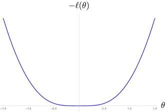
(a) Flat minimum of the negative log likelihood.

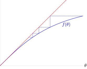
(b) Nonlinear contraction of $f(\theta)$ and the resulting sublinear rate of convergence.

Figure 1: Population version of the negative log likelihood and the EM map for $\theta_{*}=0$.

1.3 Related work

Since the original paper [DLR77], the EM algorithm has been widely used in Gaussian mixture models [RW84, XJ96]. As can be seen from its gradient ascent interpretation (13), a limiting point of the EM iteration is only guaranteed to be a critical point of the likelihood function rather than the global MLE. Various techniques for choosing the initialization has been proposed (cf. the survey [KX03] and the references therein); however, in practice random initializations are often preferred due to its simplicity over more costly approaches such as spectral methods [BCG03]. Furthermore, it is well-known in practice [RW84, KX03] that the convergence of the EM iteration can be very slow when the components are not well separated, agreeing with the theoretical findings in Theorem 1 and Theorem 2.

Recently there is a renewed interest on the EM algorithm in high dimensions from both statistical and optimization perspectives. General conditions (such as strong concavity and smoothness) are given in [BWY17] to guarantee the local convergence of the EM algorithm as well as its statistical performance. Particularized to the simple 2-GM model (4), [BWY17, Corollary 2] shows that if $\|\theta_{*}\|$ exceeds some large constant and the initialization satisfies $\|\theta_{0}-\theta_{*}\|\leq\frac{1}{4}\|\theta_{*}\|$, then with probability $1-\delta$ the EM iteration converges exponentially fast to a neighborhood at $\theta_{*}$ of radius $\sqrt{\frac{Cd}{n}\log\frac{1}{\delta}}$ for some constant $C$ depending on $\|\theta_{*}\|$. There are two major distinctions between [BWY17] and the current paper: First, the requirement on the initialization in [BWY17] is very strong, which implies that $\theta_{0}$ has a non-trivial angle with $\theta_{*}$ and clearly cannot be afforded by random initializations. Second, to bound the deviation between the sample EM trajectory and its population counterpart, [BWY17] proved that

$$\sup_{\|\theta\|\leq C}\|f_{n}(\theta)-f(\theta)\|=\widetilde{O}\left(\sqrt{\frac{d}{n}}\right)$$

with high probability, where $\widetilde{O}(\cdot)$ hides logarithmic factors. Such a concentration inequality in terms absolute deviation is too weak to yield the sharp rates in Theorem 1 and 2 even in one dimension. Instead, in order to obtain the optimal statistical and computational guarantees, it is crucial to bound the relative deviation and show that with high probability,

$$\sup_{\|\theta\|\leq C}\frac{\|f_{n}(\theta)-f(\theta)\|}{\|\theta\|}=\widetilde{O}\left(\sqrt{\frac{d}{n}}\right)$$ (20)

i.e., $f_{n}-f$ is $\widetilde{O}(\sqrt{\frac{d}{n}})$-Lipschitz, the reason being that when the iterates are close to zero, the finite-sample deviation is proportionally small as well. In addition, in Section 6 we show that the EM iterations converge to the MLE under mild conditions.

The global convergence of the population EM iterates has been analyzed in [XHM16, DTZ17]. The following deterministic result was shown: Provided that the initial value $\theta_{0}$ is not orthogonal to $\theta_{*}$, the population version of the EM iteration, that is, the sequence (8) with $f_{n}$ replaced by $f$, converges to the global maximizer of the population log likelihood $\ell$ in (12), namely, $\theta_{*}$ (resp. $-\theta_{*}$) if $\langle\theta_{0},\theta_{*}\rangle>0$ (resp. $<0$). If $\langle\theta_{0},\theta_{*}\rangle=0$, then the population EM iteration converges to $0$, the unique saddle point of $\ell$. For the sample EM, [XHM16, Theorem 7] showed that when the dimension and $\theta_{*}$ are fixed, the difference of the sample and population EM iteration vanishes in the double limit of $t\to\infty$ followed by $n\to\infty$; neither finite-sample nor finite-iteration guarantees are provided. As for high dimensions, a variant of the EM algorithm using sampling splitting is analyzed in [DTZ17] consisting of two steps: First, run EM with a random and sufficiently small initialization for $\Theta(\frac{\log d}{\|\theta_{*}\|^{2}})$ iterations. Next, renormalize the resulting estimate so that its norm is a large constant, and continue to run EM for another $\Theta(\frac{1}{\|\theta_{*}\|^{2}}\log\frac{1}{\epsilon})$ iterations. The final output achieves a loss of $\epsilon$ with high probability provided that each iteration operates on a fresh batch of $\widetilde{\Theta}(\frac{d}{\epsilon^{2}\|\theta_{*}\|^{4}})$ samples. The use of sampling splitting conveniently ensures independence among iterations and circumvents the major difficulty of analyzing the entire trajectory; however, for the desired accuracy of $\epsilon=O(\frac{1}{\|\theta_{*}\|}\sqrt{d/n})$, the total number of samples is $\widetilde{\Theta}(\frac{n}{\|\theta_{*}\|^{4}})$, which far exceeds $n$ when $\|\theta_{*}\|$ is small.

Based on the population results in [XHM16], [MBM18] showed that if $\|\theta_{*}\|$ is at least a constant, the landscape of the log likelihood $\ell_{n}$ is close to that of the population version (in terms of the critical points and the Hessian). Specifically, [MBM18, Theorem 8] showed the following: There exist constants $C,C^{\prime}$ depending on $\|\theta_{*}\|$ and $\delta$, such that if $n\geq Cd\log d$, then with probability $1-\delta$, $\ell_{n}$ has two local maxima in the ball $B(0,C^{\prime})$, which are within Euclidean distance $C\sqrt{\frac{d\log n}{n}}$ of $\pm\theta_{*}$. As a corollary of the empirical landscape analysis, with appropriately chosen parameters and initialized from any point in $B(0,C^{\prime})$, standard trust-region method (cf. e.g. [CGT00, Algorithm 6.1.1]) is guaranteed to converge to a local maximizer of $\ell_{n}$. It should be noted that trust-region method is a second-order method using the Hessian information, which is more expensive than first-order methods such as gradient descent including the EM algorithm (8). Furthermore, the number of iterations needed to reach the statistical optimum is unclear.

On the technical side, the main difficulty of analyzing a sample-driven iterative scheme, such as (8), is the dependency between the iterates $\{\theta_{t}\}$ and the data, since each iteration takes one pass over the same set of samples. Of course, one can conduct a uniform analysis by taking a supremum over the realization of $\theta_{t}$; however, since the supremum is over a $d$-dimensional space, the resulting bound is too crude to characterize the growth of the “signal” $\langle\theta_{*},\theta_{t}\rangle$, which is very close to zero initially (that is, $O_{P}(\frac{1}{\sqrt{d}})$, due to random initialization). It is for this reason that the analysis is significantly more challenging than those using sample splitting such as [BWY17, DTZ17], which sidesteps the difficulty of dependency. Furthermore, such trajectory analysis, which tracks the signal growth from random initializations, does not follow from landscape analysis.

In this vein, the most related to the current paper is the recent seminal work [CCFM19] on analyzing gradient descent for nonconvex phase retrieval with random initializations, where the goal is to recover a $d$-dimensional signal $x_{*}$ from noiseless quadratic measurements $\langle a_{i},x_{*}\rangle^{2}$ with iid Gaussian $a_{i}$. To overcome the aforementioned difficulties due to dependency, the main idea of [CCFM19] is two-fold: In addition to the commonly used “leave-one-sample-out” method that analyzes the auxiliary iteration when one measurement is replaced by an independent copy, [CCFM19] introduced a “leave-one-coordinate-out” auxiliary iteration where a single coordinate of each measurement vector is is replenished with a random sign. This is possible thanks to the rotational symmetry of the Gaussian measurement vectors, which allows one to assume, without loss of generality, that the ground truth is a coordinate vector. By comparing the auxiliary dynamics to the original one, one can effectively decouple the data and the iterates. The idea of leave-one-coordinate-out turns out to be crucial in our analysis of randomly initialized EM, where we introduce an auxiliary sequence with a randomized label but otherwise identical to the original sequence; on the other hand, we are able to conduct the analysis without resorting to the leave-one-sample-out method. Compared to [CCFM19] which relies on the strong convexity of the population objective function and the resulting contraction of the iteration, for the EM algorithm since we do not assume $\theta_{*}$ is bounded away from zero, none of these applies which creates additional challenges for the analysis.

Finally, we note that the very recent and independent work [DHK⁺18, DHK⁺19] obtained a tight analysis of the performance of EM algorithm when the true model is a single Gaussian and the postulated model is an over-specified Gaussian mixture. In particular, guarantees similar to Theorem 1 are shown for the special case of $\theta_{*}=0$, and both balanced and unbalanced mixture model are considered as well as the more general location-scale mixtures.

1.4 Notations

Throughout the paper, $c,C,C_{0},C_{1},\ldots,C^{\prime},C^{\prime\prime}$ denote constants whose values vary from place to place and only depend on an upper bound on $\|\theta_{*}\|$, and the notation $\lesssim,\gtrsim,\asymp$ are within these constant factors. Since we assume that $\|\theta_{*}\|\leq r$ for some absolute constant $r$, these constant factors are absolute as well.

Let ${\mathcal{L}}(X)$ denote the distribution (law) of a random variable $X$. The generic notation $\mathbb{E}_{n}[\cdot]$ denotes the empirical average over $n$ iid samples, namely, $\mathbb{E}_{n}[f(X)]\triangleq\frac{1}{n}\sum_{i=1}^{n}f(X_{i})$, where $X_{i}$’s are iid copies of $X$. We say a random variable $X$ is $s$-subgaussian (resp. $s$-subexponential) if $\|X\|_{\psi_{2}}\triangleq\inf\{t>0:\mathbb{E}e^{X^{2}/t^{2}}\leq 2\}\leq\sqrt{s}$ (resp. $\|X\|_{\psi_{1}}\triangleq\inf\{t>0:\mathbb{E}e^{|X|/t}\leq 2\}\leq s$).

Let $\|x\|$ denotes the Euclidean norm of a vector $x$. Let $B(x,R)$ denote the ball of radius $R$ centered at $x$ and $B(0,R)$ is abbreviated as $B(R)$. For any matrix $M$, $\left\|{M}\right\|_{{\rm op}}$ and $\|M\|_{\rm F}$ denote its operator (spectral) norm and Frobenius norm, respectively.

1.5 Organization

The rest of the paper is organized as follows. Section 2 gives the statistical and computational guarantees for EM algorithm in one dimension, showing the achievability of the optimal average risk up to constant factors. Section 3 states and proves the relative concentration result (20) for the sample EM map. Section 4 presents the analysis of the EM algorithm in $d$ dimensions and give near-optimal statistical and computational guarantees assuming a modest condition on the initialization. In Section 5 we show that starting from a single random initialization, such a condition is fulfilled in at most $O(\frac{\log n}{\|\theta_{*}\|^{2}})$ iterations with high probability. Section 6 proves the convergence of the EM iteration to the MLE. Discussions and open problems are presented in Section 7. Proofs for Sections 2–Section 6 are given in Section 8–12, respectively.

In particular, the main result Theorem 2 previously announced in Section 1.2 follows from Theorems Theorem 7 in conjunction with Theorem 8 (on random initialization) and Theorem 9 (on convergence to MLE), while Theorem 1 follows from combining Theorems 2 and 6.

Complementing the performance guarantee on the EM algorithm, Theorem 10 in Appendix B determines the minimax rates for the 2-GM model in any dimension, which may be of independent interest. Auxiliary results are given in Appendix A.

2 EM iteration in one dimension

In this section we present the analysis for one dimension which turns out to be significantly simpler than the $d$-dimensional case; nevertheless, several proof ingredients, both statistical and computational, will re-appear in the analysis for $d$ dimensions later in Section 4. To bound the relative deviation between the sample and population EM trajectories, we use the concentration inequality for empirical distributions under the Wasserstein distance. Although perhaps not crucial, this method simplifies the analysis and yields the optimal rate of the average risk without unnecessary log factors in one dimension.

2.1 Concentration via Wasserstein distance

Recall the 1-Wasserstein distance between probability distributions $\mu$ and $\nu$ [Vil03]:

$$W_{1}(\mu,\nu)=\inf\mathbb{E}|X-Y|$$

where the infimum is over all couplings of $\mu$ and $\nu$, i.e., joint law ${\mathcal{L}}(X,Y)$ such that ${\mathcal{L}}(X)=\mu$ and ${\mathcal{L}}(Y)=\nu$.

To relate the Wasserstein distance to the EM map, we start with the following simple observation:

Lemma 1.

For any $x,y\in\mathbb{R}$,

$$\sup_{\theta\in\mathbb{R}}\frac{|x\tanh(x\theta)-y\tanh(y\theta)|}{|\theta|}=|x^{2}-y^{2}|.$$

Proof.

Without loss of generality (WLOG), assume that $x\geq y\geq 0$. Then by symmetry,

$$\sup_{\theta\in\mathbb{R}}\frac{|x\tanh(x\theta)-y\tanh(y\theta)|}{|\theta|}= ~{}\sup_{\theta\geq 0}\frac{|x\tanh(x\theta)-y\tanh(y\theta)|}{\theta}$$

$$= ~{}\sup_{\theta\geq 0}\frac{x\tanh(x\theta)-y\tanh(y\theta)}{\theta}.$$ (21)

Straightforward calculation gives

$$\frac{\partial}{\partial\theta}\frac{\partial}{\partial x}\left(\frac{x\tanh(x\theta)}{\theta}\right)=\frac{1}{\theta^{2}\cosh^{2}(\theta x)}\left(\theta x-\frac{1}{2}\sinh(2\theta x)-2(\theta x)^{2}\tanh(\theta x)\right)\leq 0,$$

where the inequality follows from $\sinh(t)\geq t$ and $\tanh(t)\geq 0$ for $t\geq 0$. Therefore $\theta\mapsto\frac{\partial}{\partial x}(\frac{x\tanh(x\theta)}{\theta})$ is decreasing on $\mathbb{R}_{+}$, which implies that the supremum on the RHS of (21) is attained at $\theta=0$. ∎

By coupling, an immediate corollary to Lemma 1 is the following:

Lemma 2.

For any random variables $X$ and $Y$,

$$\sup_{\theta\in\mathbb{R}}\frac{|\mathbb{E}[Y\tanh(\theta Y)]-\mathbb{E}[X\tanh(\theta X)]|}{|\theta|}\leq W_{1}({\mathcal{L}}(X^{2}),{\mathcal{L}}(Y^{2})).$$

As mentioned earlier in Section 1.3, it is crucial to establish the relative derivation in the sense of (20) for the sample EM trajectory. Let $\Delta_{n}=f_{n}-f$, where $f_{n}$ and $f$ are the sample and population EM map defined in (9) and (10). As a consequence of Lemma 2, we have, for all $\theta\in\mathbb{R}$,

$$|\Delta_{n}(\theta)|\leq|\theta|W_{1}(\nu,\nu_{n})$$ (22)

where $\nu={\mathcal{L}}(Y^{2})$ and $\nu_{n}$ is the empirical distribution of the squared samples $Y_{1}^{2},\ldots,Y_{n}^{2}$. In other words, $\Delta_{n}$ is $W_{1}(\nu,\nu_{n})$-Lipschitz. To bound the Lipschitz constant, since $\mathbb{E}\left[\exp(Y^{2})\right]\leq C(r)$, applying the concentration inequality in [FG15, Theorems 1 and 2] (with $d=p=1$, $\alpha=2/3$, $\epsilon=1/3$ and $\gamma=1$), we have

$$\mathbb{E}\left[W_{1}(\nu,\nu_{n})\right]\leq\frac{c_{0}}{\sqrt{n}}$$ (23)

and

$$\mathbb{P}\left[W_{1}(\nu,\nu_{n})\geq x\right]\leq ~{}c_{1}[\exp(-c_{2}nx^{2}){\mathbf{1}_{\left\{{x\leq 1}\right\}}}$$

$$~{}+\exp(-c_{2}(nx)^{1/3}){\mathbf{1}_{\left\{{x\leq 1}\right\}}}+\exp(-c_{2}(nx)^{2/3})],\quad x>0$$ (24)

where $c_{0},c_{1},c_{2}$ depend only on $r$. Therefore, for any $1\lesssim a\lesssim n^{1/10}$, $\mathbb{P}[W_{1}(\nu,\nu_{n})\geq\frac{a}{\sqrt{n}}]\leq\exp(-\Omega(a^{2}))$.

2.2 Finite-sample analysis

The population EM map defined in (10) satisfies the following properties:

Lemma 3.

For any $\theta_{*}\geq 0$,

1. $\theta\mapsto f(\theta)$ is an increasing odd and bounded function on $\mathbb{R}$, with

   $$-(1+\theta_{*})\leq-\mathbb{E}|Y|=f(-\infty)\leq f(\theta)\leq f(\infty)=\mathbb{E}|Y|\leq 1+\theta_{*}.$$

2. $\theta\mapsto f(\theta)$ is concave on $\mathbb{R}_{+}$ and convex on on $\mathbb{R}_{-}$.

3. $f(0)=0$, $f^{\prime}(0)=1+{\theta_{*}}^{2}$, $f^{\prime\prime}(0)=0$, and $f^{\prime}(\theta_{*})\leq\exp(-{\theta_{*}}^{2}/2)$.

4. Define

   $$q(\theta)\triangleq\frac{f(\theta)}{\theta}$$ (25)

   Then $q$ is decreasing on $\mathbb{R}_{+}$. Furthermore, for $\theta\geq 0$,

   $$q^{\prime}(\theta)=-\mathbb{E}\left[\frac{Y\sinh(2\theta Y)-2\theta Y^{2}}{2\theta^{2}\cosh^{2}(\theta Y)}\right]\leq-\frac{2\theta}{3}\mathbb{E}\left[\frac{Y^{4}}{\cosh^{2}(\theta Y)}\right].$$ (26)

The sample-based EM iterates are given by (8), that is,

$$\theta_{t+1}=f_{n}(\theta_{t}).$$

Here the samples $Y_{1},\ldots,Y_{n}$ are iid drawn from $P_{\theta_{*}}=\frac{1}{2}N(-\theta_{*},1)+\frac{1}{2}N(\theta_{*},1)$. By the global assumption (31), we have $0\leq\theta_{*}\leq r$. WLOG, we assume that $\theta_{0}>0$ for otherwise we can apply the same analysis to the sequence $\{-\theta_{t}\}$. By (22), $\Delta_{n}=f-f_{n}$ is $w_{n}$-Lipschitz, where $w_{n}\triangleq W_{1}(\nu,\nu_{n})$ is a random variable. Define the high-probability event

$$E=\{W_{1}(\nu,\nu_{n})\leq c_{w}\},$$ (27)

where $c_{w}$ is a small constant depending only on $r$ that satisfies $c_{w}<\frac{1}{4}$. By (24), we have $\mathbb{P}\left[E\right]\geq 1-\exp(-\Omega(n^{1/3}))$.

Define the following auxiliary iterations:

$$\begin{cases}\theta^{\texttt{+}}_{t+1}=f(\theta^{\texttt{+}}_{t})+w_{n}\theta^{\texttt{+}}_{t}\\ \theta^{\texttt{-}}_{t+1}=f(\theta^{\texttt{-}}_{t})-w_{n}\theta^{\texttt{-}}_{t}\end{cases},\qquad\theta^{\texttt{+}}_{0}=\theta^{\texttt{-}}_{0}=\theta_{0}.$$ (28)

By Lemma 3, $q$ is decreasing and maps $\mathbb{R}_{+}$ onto $(0,1+\theta_{*}^{2}]$. Define

$$\theta^{\texttt{+}}\triangleq ~{}q^{-1}\left(1-w_{n}\right)$$ (29)

$$\theta^{\texttt{-}}\triangleq ~{}\begin{cases}q^{-1}\left(1+w_{n}\right)&|\theta_{*}|\geq\sqrt{w_{n}}\\ 0&|\theta_{*}|<\sqrt{w_{n}}\end{cases}.$$ (30)

We will show that on the high-probability event (27), the EM iterates $\{\theta_{t}\}$ is sandwiched between the two auxiliary iterates $\{\theta^{\texttt{+}}_{t}\}$ and $\{\theta^{\texttt{-}}_{t}\}$ (see Fig. 2). This is made precisely by the following theorem, which gives the estimation error bound and finite-iteration guarantees for the EM algorithm in one dimension:

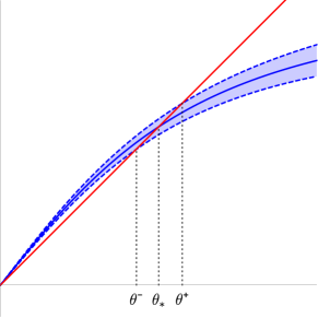
Figure 2: Perturbed EM trajectory and fixed points.

Theorem 3 (Statistical and computational guarantees for one-dimensional EM).

Assume that

$$0\leq\theta_{*}\leq r$$ (31)

for some constant $r$. Assume that

$$0<\theta_{0}\leq r_{0}.$$

Then there exist constants $\tau_{1},\ldots,\tau_{5}$ depending on $r$ only, and a constant $n_{0}=n_{0}(r,r_{0})$, such that for all $n\geq n_{0}$, on the event (27), the following holds:

1. For all $t\geq 0$,

   $$0\leq\theta^{\texttt{-}}_{t}\leq\theta_{t}\leq\theta^{\texttt{+}}_{t}\leq\tau_{1}.$$ (32)

2. $$\ell(\theta_{t},\theta_{*})\leq\tau_{2}\min\left\{\frac{w_{n}}{\theta_{*}},\sqrt{w_{n}}\right\},$$ (33)

   holds for all $t\geq T=T(\theta_{0},\theta_{*},w_{n})$, where

   $$T=\begin{cases}\frac{\tau_{3}}{w_{n}}&\theta_{*}\leq\tau_{4}\sqrt{w_{n}}\\ \frac{\tau_{3}}{\theta_{*}^{2}}\log\frac{1}{\theta_{0}w_{n}}&\theta_{*}\geq\tau_{4}\sqrt{w_{n}}.\end{cases}$$ (34)

A corollary of Theorem 3 is the following guarantee on the average risk:

Corollary 1.

There exist constants $c_{1},c_{2}$ depending only on $r$, such that

$$\mathbb{E}[\ell(\theta_{t},\theta_{*})]\leq c_{1}\min\left\{\frac{1}{\theta_{*}\sqrt{n}},\frac{1}{n^{1/4}}\right\},$$ (35)

holds for all

$$t\geq c_{2}\min\left\{\sqrt{n},\frac{1}{\theta_{*}^{2}}\right\}\log\frac{n}{\theta_{0}}.$$ (36)

Remark 2.

The rate in (35) is optimal in the following sense: the second term $n^{-1/4}$ matches the minimax lower bound in Appendix B, while the first term corresponds to the local minimax rate since the Fisher information behaves as $\Theta(\theta_{*}^{2})$ for small $\theta_{*}$. Indeed, we will show in Section 6 that the EM iteration converges to the MLE which is asymptotic efficient.

In the special case of $\theta_{*}=0$, results similar to Theorem 3 have been shown in [DHK⁺18, Theorem 3]. Furthermore, [DHK⁺18, Theorem 4] provided a matching lower bound showing that any limiting point of the EM iteration is $\Omega(n^{-1/4})$ with constant probability.

Computationally, suppose we initialize with $\theta_{0}=1$. Then regardless of the value of $\theta_{*}$, we have the worst-case computational guarantee: with high probability, the EM algorithm achieves the optimal rate (35) in at most $O(\sqrt{n}\log n)$ iterations. The number of needed iterations can be pre-determined on the basis of $n$ and $\theta_{0}$, without knowing $\theta_{*}$.

3 Concentration of the EM trajectory: relative error bound

Recall that $\Delta_{n}=f-f_{n}$ denotes the difference between the sample and the population EM maps. In one dimension, we have shown that the random function $\Delta_{n}:\mathbb{R}\to\mathbb{R}$ is $O_{P}(\frac{1}{\sqrt{n}})$-Lipschitz by means of the Wasserstein distance between the empirical distribution and the population. The goal of this section is to extend this result to $d$ dimensions, by showing with high probability $\Delta_{n}:\mathbb{R}^{d}\to\mathbb{R}^{d}$ is $O(\sqrt{\frac{d\log n}{n}})$-Lipschitz with respect to the Euclidean distance on a ball of radius $R=\Theta(\sqrt{d})$. Since with high probability the EM map $f_{n}$ takes values within this radius, this result allows us to control the fluctuation of the EM trajectory with respect to its population counterpart proportionally to the distance to the origin. This relative error bound given next is crucial for obtaining the optimal statistical and computational guarantees.

Theorem 4.

Assume that $\|\theta_{*}\|\leq r$ and

$$n\geq Cd\log d$$

for some universal constant $C$. There exist universal constants $c_{0},C_{0}$, such that with probability at least $1-\exp(-c_{0}d\log n)$,

1. For all $\theta\in\mathbb{R}^{d}$, $f_{n}(\theta)\in B(R)$ where $R=10(\sqrt{d}+r)$.

2. The function $\Delta_{n}$ is $L$-Lipschitz on $B(R)$, where $L=C_{0}(1+r)\sqrt{\frac{d}{n}\log n}$.

The proof is given in Section 9. We note that it is straightforward to extend the argument in one dimension (cf. (22)–(23)) to bound the Lipschitz constant of $\Delta_{n}$ by the Wasserstein (in fact, $W_{2}$) distance between the empirical distribution and the population. Nevertheless, it is well-known that the Wasserstein distance suffers from the curse of dimensionality; for example, the $W_{1}$ distance behaves as $O_{P}(n^{-\frac{1}{d}})$ (cf. e.g [Tal94, FG15]). This effect is due to the high complexity of Lipschitz functions in $d$ dimensions. In contrast, the EM map (9) depends on the $d$-dimensional randomness only through its linear projection, which suggests that the it is possible to obtain a rate close to $\sqrt{\frac{d}{n}}$.

4 Analysis in $d$ dimensions

In this section we analyze for the EM algorithm in high dimensions. By using properties of the population EM iteration in Section 4.1 and the relative deviation bound in Section 3, in Section 4.2 we prove optimal statistical and computational guarantees for the sample EM iteration, assuming a modest condition on the initialization which is much weaker than those in [BWY17]. Although not necessarily satisfied by random initialization, later in Section 5 we show that randomly initialized EM iteration will eventually fulfill such a condition with high probability.

4.1 Properties of the population EM map

Consider the population version of the EM iterates, driven by the population EM map (10):

$$\boldsymbol{\theta}_{t+1}=f(\boldsymbol{\theta}_{t}),\qquad\boldsymbol{\theta}_{0}=\theta_{0}.$$

We use bold face to delineate it from the finite-sample iteration (8). Let $\eta_{*}=\theta_{*}/\|\theta_{*}\|$. Let

$$\theta_{0}=\alpha_{0}\eta_{*}+\beta_{0}\xi_{0},$$

where $\xi_{0}\perp\theta_{*}$ and $\|\xi_{0}\|=1$, so that $\mathrm{span}(\theta_{0},\theta_{*})=\mathrm{span}(\eta_{*},\xi)$. The next lemma shows that the population EM iterates cannot escape the two-dimensional subspace spanned by $\theta_{*}$ and $\theta_{0}$:

Lemma 4.

For each $t\geq 1$,

$$\boldsymbol{\theta}_{t}\in\mathrm{span}(\theta_{*},\theta_{0}).$$ (37)

Furthermore, let

$$\boldsymbol{\theta}_{t}=\boldsymbol{\alpha}_{t}\eta_{*}+\boldsymbol{\beta}_{t}\boldsymbol{\xi}_{t}$$

where $\boldsymbol{\xi}_{t}\perp\eta_{*}$ and $\|\boldsymbol{\xi}_{t}\|=1$. Then $\{(\boldsymbol{\alpha}_{t},\boldsymbol{\beta}_{t})\}$ satisfies the following recursion

$$\boldsymbol{\alpha}_{t+1}= ~{}F(\boldsymbol{\alpha}_{t},\boldsymbol{\beta}_{t})$$ (38)

$$\boldsymbol{\beta}_{t+1}= ~{}G(\boldsymbol{\alpha}_{t},\boldsymbol{\beta}_{t})$$ (39)

where

$$F(\alpha,\beta)\triangleq ~{}\mathbb{E}[V\tanh(\alpha V+\beta W)]$$ (40)

$$G(\alpha,\beta)\triangleq ~{}\mathbb{E}[W\tanh(\alpha V+\beta W)]$$ (41)

with $W\sim N(0,1)$ and $V\sim\frac{1}{2}N(\pm\|\theta_{*}\|,1)$ being independent.

Proof.

It suffices to show (37), which was proved in [XHM16]. To give some intuitions, we provide a simple argument below by induction on $t$. Clearly (37) holds for $t=0$. Next, fix any $u\in\mathrm{span}(\theta_{*},\theta_{0})^{\perp}$. By the induction hypothesis, $u\perp\boldsymbol{\theta}_{t}$. Therefore

$$\langle u,\boldsymbol{\theta}_{t+1}\rangle=\mathbb{E}[\langle u,Y\rangle\tanh(\langle Y,\boldsymbol{\theta}_{t}\rangle)]=\mathbb{E}[\langle u,Z\rangle\tanh(\langle\theta_{*},\boldsymbol{\theta}_{t}\rangle X+\langle Z,\boldsymbol{\theta}_{t}\rangle)]=0$$

since $\langle u,Z\rangle,\langle\boldsymbol{\theta}_{t},Z\rangle$ and $X$ are mutually independent. This proves (37) holds for $t+1$. ∎

Next, we analyze the convergence of $(\boldsymbol{\alpha}_{t},\boldsymbol{\beta}_{t})$. Without loss of generality (otherwise we can negate $\theta_{*}$ and $\xi$), we assume that

$$\boldsymbol{\alpha}_{0}\geq 0,\quad\boldsymbol{\beta}_{0}\geq 0.$$

Therefore $\boldsymbol{\theta}_{t}\to\theta_{*}$ is equivalent to $\boldsymbol{\alpha}_{t}\to\|\theta_{*}\|$ and $\boldsymbol{\beta}_{t}\to 0$. The convergence is easily justified by the following lemma:

Lemma 5 (Properties of $F$ and $G$).

For any $\alpha$ and $\beta\geq 0$,

1. $\alpha\mapsto F(\alpha,\beta)$ is increasing, odd, concave (resp. convex) on $\mathbb{R}_{+}$ (resp. $\mathbb{R}_{-}$), with $F(0,\beta)=0$, $F(\pm\|\theta_{*}\|,0)=\pm\|\theta_{*}\|$.

2. $F(\alpha,\beta)\geq 0$ for any $\alpha\geq 0$.

3. $\beta\mapsto G(\alpha,\beta)$ is increasing and concave, with $G(\alpha,0)=0$.

4. $\alpha\mapsto G(\alpha,\beta)$ is even, decreasing on $\mathbb{R}_{+}$; $\beta\mapsto F(\alpha,\beta)$ is decreasing for $\alpha\geq 0$ and increasing for $\alpha\leq 0$.

5. (Boundedness)

   $$|F(\alpha,\beta)|\leq\|\theta_{*}\|+\sqrt{2/\pi},\quad 0\leq G(\alpha,\beta)\leq\sqrt{2/\pi}.$$

6. $$G(\alpha,\beta)\leq ~{}G(0,\beta)=\mathbb{E}[W\tanh(\beta W)].$$ (42)

7. $$f(\alpha)\geq F(\alpha,\beta)\geq f(\alpha)-(1+\|\theta_{*}\|^{2})\alpha\beta^{2}, \qquad\alpha\geq 0$$ (43)

   $$f(\alpha)\leq F(\alpha,\beta)\leq f(\alpha)-(1+\|\theta_{*}\|^{2})\alpha\beta^{2}, \qquad\alpha\leq 0$$ (44)

   where

   $$f(\alpha)\triangleq F(\alpha,0)=\mathbb{E}[V\tanh(\alpha V)]$$ (45)

   coincides with the one-dimensional EM map defined in (10) with $\theta_{*}$ replaced by $\|\theta_{*}\|$.

8. $$G(\alpha,\beta)\leq\beta\left(1-\frac{\alpha^{2}+\beta^{2}}{2+4(\alpha^{2}+\beta^{2})}\right).$$ (46)

From Lemma 5 it is clear that in the population case, the only fixed points are the desired $(\pm\|\theta_{*}\|,0)$ and undesired $(0,0)$. As long as the initial value is not orthogonal to the ground truth (i.e., $\boldsymbol{\alpha}_{0}\neq 0$), $\boldsymbol{\theta}_{t}$ converges to $\pm\theta_{*}$; this has been previously shown in [XHM16, DTZ17]. In fact, the orthogonal component $\boldsymbol{\beta}_{t}$ converges to $0$ monotonically regardless of the signal component $\boldsymbol{\alpha}_{t}$. Furthermore, if we start out with $\boldsymbol{\alpha}_{0}>0$, then $\boldsymbol{\alpha}_{t}>0$ remains true for all $t$, and when $\boldsymbol{\beta}_{t}$ gets sufficiently close to 0, $\boldsymbol{\alpha}_{t}$ converges to $\|\theta_{*}\|$ following the one-dimensional EM dynamics (cf. (45)). However, a major distinction between the one-dimensional and $d$-dimensional case is that $\boldsymbol{\alpha}_{t}$ need not converge monotonically even in the infinite-sample setting. In fact, if the initial value has little overlap with the ground truth (as is the case for random initialization in high dimensions), $\boldsymbol{\beta}_{t}$ is large initially which causes $\boldsymbol{\alpha}_{t}$ to decrease and $\boldsymbol{\theta}_{t}$ to move closer to the undesired fixed point at zero (see Fig. 3(a)). Therefore, in the finite-sample setting, we need to assume conditions on the initialization (namely lower bound on $|\alpha_{t}|$) in order to avoid being trapped near zero – we will return to this point in the finite-sample analysis in the next subsection. This is in stark contrast to the one-dimensional case: even with finite samples, for any non-zero initialization, the EM iteration eventually converges to a neighborhood of the ground truth with optimal accuracy (cf. Theorem 3).

(a) Non-monotone convergence of $\boldsymbol{\alpha}_{t}$ ($\boldsymbol{\alpha}_{0}=0.1$, $\boldsymbol{\beta}_{0}=0.7$).

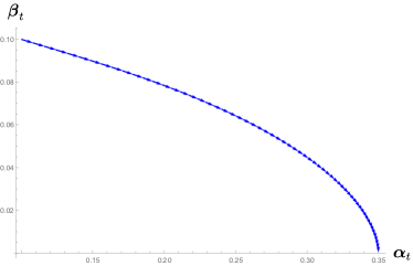
(b) Monotone convergence of $\boldsymbol{\alpha}_{t}$ ($\boldsymbol{\alpha}_{0}=\boldsymbol{\beta}_{0}=0.1$).

Figure 3: Convergence of $(\boldsymbol{\alpha}_{t},\boldsymbol{\beta}_{t})$ in the population dynamics in $d$ dimensions with $\|\theta_{*}\|=0.35$ for $60$ iterations.

4.2 Finite-sample analysis

We now analyze the $n$-sample EM iteration (8), that is,

$$\theta_{t+1}=f_{n}(\theta_{t}).$$

Write

$$\theta_{t}=\alpha_{t}\eta_{*}+\beta_{t}\xi_{t},$$

where $\xi_{t}\perp\eta_{*}=\frac{\theta_{*}}{\|\theta_{*}\|}$, $\|\xi_{t}\|=1$ and $\beta_{t}\geq 0$. Thus $\|\theta_{t}\|=\sqrt{\alpha_{t}^{2}+\beta_{t}^{2}}$.

Recall that $\Delta_{n}=f_{n}-f$ denotes the difference between the sample and population EM maps. In view of Theorem 4, with probability at least $1-\exp(-c_{0}d\log n)$, the following event holds:

$$\sup_{\theta\in\mathbb{R}^{d}}\|f_{n}(\theta)\| ~{}\leq R$$ (47)

$$\|\Delta_{n}(\theta)\| ~{}\leq\omega\|\theta\|,\quad\forall\theta\in B(R),$$

where $R=10(r+\sqrt{d})$ and

$$\omega=\sqrt{C_{\omega}\frac{d}{n}\log n}$$ (48)

and $C_{\omega}$ is a constant that only depends on $r$. We assume that $n$ is sufficiently large so that $\omega$ is at most an absolute constant.

Recall from Lemma 4 that $f(\theta)\in\mathrm{span}(\eta_{*},\theta)$ for any $\theta\in\mathbb{R}^{d}$. Furthermore,

$$f(\theta_{t})=F(\alpha_{t},\beta_{t})\eta_{*}+G(\alpha_{t},\beta_{t})\xi_{t},$$

where $F$ and $G$ are defined in (40)–(41). Therefore

$$\alpha_{t+1}=\left\langle\theta_{t+1},\eta_{*}\right\rangle=F(\alpha_{t},\beta_{t})\eta_{*}+\langle\Delta_{n}(\theta_{t}),\eta_{*}\rangle.$$

In view of (47), we have

$$|\langle\Delta_{n}(\theta_{t}),\eta_{*}\rangle|\leq\|\Delta_{n}(\theta_{t})\|\leq\omega(|\alpha_{t}|+\beta_{t}).$$

Hence

$$\alpha_{t+1}\leq ~{}F(\alpha_{t},\beta_{t})+\omega(|\alpha_{t}|+\beta_{t})$$ (49)

$$\alpha_{t+1}\geq ~{}F(\alpha_{t},\beta_{t})-\omega(|\alpha_{t}|+\beta_{t})$$ (50)

On the other hand, we have

$$(I-\eta_{*}\eta_{*}^{\top})\theta_{t+1}=G(\alpha_{t},\beta_{t})\xi_{t}+(I-\eta_{*}\eta_{*}^{\top})\Delta_{n}(\theta_{t}).$$

Taking norms on both sides, we have

$$\beta_{t+1}\leq ~{}G(\alpha_{t},\beta_{t})+\omega(|\alpha_{t}|+\beta_{t}).$$ (51)

The equations (49)–(50) and (51) should be viewed as the finite-sample perturbation of the population dynamics (38) and (39), respectively.

We will show that the orthogonal component $\beta_{t}$ unconditionally converges to $O(\sqrt{\omega})=O((\frac{d\log n}{n})^{\frac{1}{4}})$; however, for finite sample size we cannot expect $\beta_{t}$ to converge to zero. To analyze $\alpha_{t}$, let us assume that $\beta_{t}$ have converged to this limiting value (in fact, by initializing near zero, we can ensure $\beta_{t}=O(\sqrt{\omega})$ for all $t$.) Following the sandwich analysis in one dimension, we can define the auxiliary iterations similar to (28)

$$\begin{cases}\alpha^{\texttt{+}}_{t+1}=F(\alpha^{\texttt{+}}_{t},\beta_{t})+\omega\alpha^{\texttt{+}}_{t}+\omega^{3/2}\\ \alpha^{\texttt{-}}_{t+1}=F(\alpha^{\texttt{-}}_{t},\beta_{t})-\omega\alpha^{\texttt{-}}_{t}-\omega^{3/2}\end{cases},\qquad\alpha^{\texttt{+}}_{0}=\alpha^{\texttt{-}}_{0}=\alpha_{0}$$ (52)

and show that the upper bound sequence $\{\alpha^{\texttt{+}}_{t}\}$ converges to $\alpha^{\texttt{+}}$ which is within the optimal rate of the desired $\|\theta_{*}\|$. However, due to the additional intercept, the lower bound sequence $\{\alpha^{\texttt{-}}_{t}\}$ have two possible fixed points (see Fig. 4): the “good” fixed point $\alpha^{\texttt{-}}$ that is within the optimal rate of $\|\theta_{*}\|$, and the “bad” fixed point $\alpha^{\circ}$ that is close to zero (in fact, $\alpha^{\circ}=O(\sqrt{\omega})$).

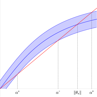
Figure 4: Perturbed EM trajectory for $\alpha_{t}$ and fixed points.

Consequently, if the iteration starts from from the left of the bad fixed points, i.e., $\alpha_{0}<\alpha^{\circ}$, which is what happens when the initialization is nearly orthogonal to $\theta_{*}$, the lower bound sequence $\alpha^{\texttt{-}}_{t}$ may be stuck at near zero and fail to converge to the desired neighborhood of $\|\theta_{*}\|$. Thus to rule this out it requires more refined argument than the above sandwich analysis, which is carried out in the next section. For this section we focus on proving the performance guarantee assuming a mild assumption on the initialization. Specifically, we establish the following claims:

1. Orthogonal direction: we show that regardless of the initialization, $\{\beta_{t}\}$ unconditionally converges to the near-optimal rate $O(\sqrt{\omega})$. In particular, if we start from near zero (and we will), we can ensure that the entire sequence $\{\beta_{t}\}$ is $O(\sqrt{\omega})$ for all $t$.

2. Signal direction: we show that

   • For small $\theta_{*}$, i.e., $\|\theta_{*}\|=O(\sqrt{\omega})$, $\{|\alpha_{t}|\}$ unconditionally converges to $O(\sqrt{\omega})$, and hence so does $\|\theta_{t}-\theta_{*}\|$.

   • For large $\theta_{*}$, i.e., $\|\theta_{*}\|=\Omega(\sqrt{\omega})$, provided that the initialization satisfies

     $$|\langle\eta_{0},\eta_{*}\rangle|\gtrsim\frac{1}{\|\theta_{*}\|^{2}}\sqrt{\frac{d}{n}\log n},$$

     the signal part $\{\alpha_{t}\}$ converges to $\|\theta_{*}\|+O(\frac{1}{\|\theta_{*}\|}\sqrt{\frac{d}{n}\log n})$. The condition on the initialization improves that of [BWY17], which requires that $|\langle\eta_{0},\eta\rangle|\geq\Omega(1)$ and $\|\theta_{*}\|=\Omega(1)$. Note that if $\eta_{0}$ is drawn uniformly from the unit sphere, we have $|\left\langle\eta_{0},\eta_{*}\right\rangle|=\Theta_{P}(\frac{1}{\sqrt{d}})$. Thus, in the special case of $\|\theta_{*}\|$ being a constant, the above condition is fulfilled when $n=\widetilde{\Omega}(d^{2})$. Nevertheless, in Section 5 we will prove the refined result that as long as $n=\widetilde{\Omega}(d)$, starting from a single random initialization, the EM iterates will eventually satisfy the above condition with high probability.

In the rest of the paper, we always assume that the initialization lies in a bounded ball. To simplify the presentation, assume that

$$\|\theta_{0}\|\leq 1.$$ (53)

The following theorems are the main result of this section. We note that results similar to Theorems 5–6 have been shown in [DHK⁺18, Theorem 3] in the special case of $\theta_{*}=0$.

Theorem 5 (Unconditional convergence of $\beta_{t}$).

There exist constants $\kappa_{0},\kappa_{1},\kappa_{2}$ depending only on $r$, such that on the event (47), the following holds.

1. For all $t\geq 0$,

   $$\beta_{t+1}\leq\beta_{t}(1+\omega)+\omega|\alpha_{t}|\\$$ (54)

   and

   $$\beta_{t+1}\leq\beta_{t}(1+\omega)-\frac{\beta_{t}^{3}}{2+8\Gamma^{2}}+\min\left\{\frac{\omega^{2}(2+8\Gamma^{2})}{2\beta_{t}},\omega\Gamma\right\}\\$$ (55)

   where $\Gamma=2+2r$.

2. Consequently, regardless of $\theta_{0}$,

   $$\limsup_{t\to\infty}\beta_{t}\leq\kappa_{1}\left(\frac{d}{n}\log n\right)^{\frac{1}{4}}.$$ (56)

3. Furthermore, if $\omega\leq\kappa_{0}$ and

   $$\|\theta_{0}\|\leq\kappa_{2}\left(\frac{d}{n}\log n\right)^{\frac{1}{4}},$$ (57)

   then for all $t\geq 0$,

   $$\beta_{t}\leq\kappa_{2}\left(\frac{d}{n}\log n\right)^{\frac{1}{4}}.$$ (58)

Theorem 6 (Small $\|\theta_{*}\|$: Unconditional convergence of $\alpha_{t}$).

There exist absolute constants $K,L\geq 1$, such that on the event (47), the following holds. Let $s_{0}$ be such that $K\sqrt{\omega}\leq s_{0}\leq 1$. Assume that $\|\theta_{*}\|\leq s_{0}$.

1. Regardless of $\theta_{0}$,

   $$\limsup_{t\to\infty}|\alpha_{t}|\leq 2s_{0}.$$ (59)

   and hence

   $$\limsup_{t\to\infty}\ell(\theta_{t},\theta_{*})\leq 3s_{0}+\kappa_{1}\left(\frac{d}{n}\log n\right)^{\frac{1}{4}}.$$ (60)

2. Furthermore, if the initializer $\theta_{0}$ satisfies (57), then

   $$|\alpha_{t}|\leq Ls_{0}$$ (61)

   and

   $$\ell(\theta_{t},\theta_{*})\leq 2Ls_{0}$$ (62)

   hold for all $t\geq 0$.

Theorem 7 (Large $\|\theta_{*}\|$: Conditional convergence of $\alpha_{t}$).

There exist constants $\lambda_{0},\ldots,\lambda_{4}$ depending only on $r$, such that on the event (47), the following holds. Assume that $\|\theta_{*}\|\geq\lambda_{0}\sqrt{\omega}$. Let $\eta_{0}\in S^{d-1}$ satisfies

$$|\left\langle\eta_{0},\eta_{*}\right\rangle|\geq\frac{\lambda_{2}}{\|\theta_{*}\|^{2}}\sqrt{\frac{d}{n}\log n}.$$ (63)

Set

$$\theta_{0}=c\left(\frac{d}{n}\log n\right)^{1/4}\eta_{0}$$ (64)

where $c\leq\kappa_{2}$ and $\kappa_{2}$ is from Theorem 5. Then

$$\limsup_{t\to\infty}\big{|}\alpha_{t}-\|\theta_{*}\|\big{|}\leq\lambda_{1}\frac{1}{\|\theta_{*}\|}\sqrt{\frac{d\log n}{n}}$$ (65)

and

$$\limsup_{t\to\infty}\ell(\theta_{t},\theta_{*})\leq\lambda_{3}\frac{1}{\|\theta_{*}\|}\sqrt{\frac{d\log n}{n}}.$$ (66)

Furthermore, (65) and (66) hold to all $t\geq\lambda_{4}\frac{\log n}{\|\theta_{*}\|^{2}}$.

Remark 3.

We can take $s_{0}=\lambda_{0}\sqrt{\omega}$ in Theorem 6, so that Theorems 6 and 7 gives the near-optimal rate of $O(\left(\frac{d}{n}\log n\right)^{1/4})$ for the case of small and large $\|\theta_{*}\|$ respectively. Later in the refined analysis in Section 5 we will take $s_{0}$ slightly larger than $\sqrt{\omega}$; cf. (67).

Theorems 5–7 are proved in Section 10.1. Here we give a sketch of the proof of Theorem 7. The analysis consists of three phases:

Phase I: $\alpha_{t}\lesssim\sqrt{\omega}$.

By using the condition (63) on the initialization, we show that in this phase $\alpha_{t}$ increases geometrically according to

$$\alpha_{t+1}\geq(1+\Omega(\|\theta_{*}\|^{2}))\alpha_{t}.$$

Phase II: $\alpha_{t}\gtrsim\sqrt{\omega}$.

Now that $\alpha_{t}$ has escaped the undesired fixed point near zero (cf. Fig. 4), one can apply the “sandwich bound” (52) to show that $\alpha_{t}$ follows a perturbed one-dimensional EM evolution

$$\alpha_{t+1}=f(\alpha_{t})+O(\omega\alpha_{t}),$$

where $f$ is defined (45) and coincides with the one-dimensional EM map (10) with $\theta_{*}$ replaced by $\|\theta_{*}\|$.

Phase III: $\alpha_{t}\asymp\|\theta_{*}\|$.

Recall that Theorem 5 ensures that $\beta_{t}$ converges to the worst-case rate $O(\sqrt{\omega})$. Now that $\alpha_{t}$ has reached a constant fraction of the desired limit $\|\theta_{*}\|$, we can obtain improved estimate $\beta_{t}\lesssim\frac{\omega}{\|\theta_{*}\|}$, leading to the optimal $\|\theta_{*}\|$-dependent bound (66).

5 Refined analysis for random initialization: the initial phase

In this section we analyze the EM iterates starting from a single random initialization. Since Theorems 5 and 6 have covered the case of small $\|\theta_{*}\|$, we only consider the case where $\|\theta_{*}\|\gg(\frac{d}{n})^{1/4}$. We provide a refined analysis of Phase I in the proof of Theorem 7: if the initial direction is uniformly chosen at random, then with high probability, the iterates will satisfy $\alpha_{t}=\Omega(\sqrt{\omega})$ for sufficiently large constant $C$ in at most $O(\frac{1}{\|\theta_{*}\|^{2}}\log n)$ iterations and hence the analysis in the subsequent Phase II and III applies. This was previously shown in Theorem 7 under the stronger assumption (63) which need not be fulfilled by random initializations.

Recall that $\eta_{*}=\frac{1}{\|\theta_{*}\|}\theta_{*}$ denotes the true direction and

$$\alpha_{t}=\left\langle\theta_{t},\eta_{*}\right\rangle,\quad\beta_{t}=\|(I-\eta_{*}\eta_{*}^{\top})\theta_{t}\|.$$

WLOG, we assume the following:

1. Thanks to the rotational invariance of the Gaussian distribution, we can assume that the true center is aligned with a coordinate vector, i.e., $\theta_{*}=\|\theta_{*}\|e_{1}$, so that

   $$\alpha_{t}=\theta_{t,1},\quad\beta_{t}=\|\theta_{t,\perp}\|=\|(\theta_{t,2},\ldots,\theta_{t,d})\|.$$

2. The initialization satisfies $\alpha_{0}>0$. Otherwise, we can apply the same analysis to $\{-\theta_{t}\}$ which has the same law as $\{\theta_{t}\}$.

Furthermore, we assume that the ground truth satisfies

$$r\geq\|\theta_{*}\|\geq\left(\frac{C_{\star}d\log^{3}n}{n}\right)^{1/4}$$ (67)

for some absolute constant $C_{\star}$. Otherwise, applying Theorem 6 (with $s_{0}$ being the RHS of (67)) shows that regardless of the initialization, we achieve the near optimal rate for all $t\geq 0$:

$$\|\theta_{t}-\theta_{*}\|=O\left(\left(\frac{d}{n}\log^{3}n\right)^{1/4}\right).$$ (68)

Define

$$T_{1}\triangleq\min\left\{t\in\mathbb{N}:\alpha_{t}>C_{*}\sqrt{\omega}\right\},$$ (69)

where $C_{*}$ is some constant depending only on $r$; cf. (115). The main result of this section is the following:

Theorem 8.

Assume that $\theta_{*}$ satisfies (67). There exists constants $C_{0},C_{1},C_{2}$ depending only on $r$, such that the following holds: Let

$$\theta_{0}=C_{0}\left(\frac{d}{n}\log n\right)^{1/4}\eta_{0},$$ (70)

where $\eta_{0}$ is drawn uniformly at random from the unit sphere $S^{d-1}$. Assume that

$$n\geq C_{1}d\log^{3}d.$$ (71)

Then with probability at least $1-\frac{C_{2}\log\log n}{\sqrt{\log n}}$,

$$T_{1}\leq T_{\star}\triangleq\frac{C_{T}(\log d+\log\log n)}{\|\theta_{*}\|^{2}}$$ (72)

where $C_{T}$ is some universal constant.

Theorem 8 shows that after $t\geq T_{1}$, the iteration enters Phase II and the statistical guarantee in Theorem 7 applies to all subsequent iterations; in particular, the optimal estimation error is achieved in another $O(\frac{\log n}{\|\theta_{*}\|^{2}})=O(\sqrt{\frac{n}{d\log n})}$ iterations, proving Theorem 2 previously announced in Section 1.2. Finally, since the case of $\|\theta_{*}\|=O((\frac{d\log^{3}n}{n})^{1/4})$ is covered by (68), the worst-case result in Theorem 1 follows.

5.1 Proof of Theorem 8

In this subsection we provide the main argument for proving Theorem 8, with key lemmas proved in Section 11.1. Suppose, for the sake of contradiction, that $\alpha_{t}\leq\sqrt{\omega}$ for all $t\leq T_{\star}$. Then in view of (58), we conclude that for all $t\leq T_{\star}$,

$$\|\theta_{t}\|\leq 2C_{1}\left(\frac{d}{n}\log n\right)^{1/4}$$ (73)

for some constant $C_{1}$. In particular, $\theta_{t}$ belongs to the unit ball in view of the assumption (71).

We now introduce an auxiliary sequence of iterates $\{\widetilde{\theta}_{t}\}$, which is main apparatus for analyzing the initial growth of the signal. Since the law of $Y_{i,1}$ is symmetric, with loss of generality, we view the $i$th sample as $Y_{i}=(b_{i}Y_{i,1},Y_{i,2},\ldots,Y_{i,d})$, where $b_{i}$’s are independent Rademacher variables, and the sample-based EM iterates is

$$\theta_{t+1}=f_{n}(\theta_{t}),$$

where

$$f_{n}(\theta)=\mathbb{E}_{n}[Y\tanh\left\langle\theta,Y\right\rangle]=\frac{1}{n}\sum_{i=1}^{n}Y_{i}\tanh\left\langle\theta,Y_{i}\right\rangle.$$

In comparison, the auxiliary iteration is based on the modified samples $({\widetilde{Y}}_{1},\ldots,{\widetilde{Y}}_{n})$, where ${\widetilde{Y}}_{i}=({\widetilde{b}}_{i}Y_{i,1},Y_{i,2},\ldots,Y_{i,d})$, ${\widetilde{b}}_{i}$’s are independent Rademacher variables, and $\{{\widetilde{b}}_{i},b_{i},Y_{i}\}$ are mutually independent. Define the auxiliary iterates

$$\widetilde{\theta}_{t+1}=\widetilde{f}_{n}(\widetilde{\theta}_{t}),$$ (74)

where

$$\widetilde{f}_{n}(\theta)\triangleq ~{}\mathbb{E}_{n}[{\widetilde{Y}}\tanh\langle\theta,{\widetilde{Y}}\rangle]=\frac{1}{n}\sum_{i=1}^{n}\widetilde{Y}_{i}\tanh\langle\theta,\widetilde{Y}_{i}\rangle.$$ (75)

Both the main and the auxiliary sequence starts from the same random initialization:

$$\widetilde{\theta}_{0}=\theta_{0},$$

as specified by (70). The angle of a random initialization satisfies the following:

Lemma 6 (Random initialization).

There exist an absolute constant $C_{0}$, such that for any $a>0$, $\mathbb{P}[|\langle\eta_{0},e_{1}\rangle|\geq\frac{a}{\sqrt{d}}]\leq C_{0}a\sqrt{\log\frac{1}{a}}$.

Proof.

Note that $\left\langle\eta_{0},e_{1}\right\rangle$ is equal in distribution to $Z_{1}/\|Z\|$, where $Z=(Z_{1},\ldots,Z_{d})$ is standard normal. Therefore $\mathbb{P}[|\langle\eta_{0},e_{1}\rangle|<\frac{a}{\sqrt{d}}]\leq\mathbb{P}[\|Z\|\geq\sqrt{Cd}]+\mathbb{P}[|Z_{1}|<\sqrt{C}a]$. Take $C=2+3\log\frac{1}{a}$. By Lemma 20, $\mathbb{P}[\|Z\|\geq\sqrt{Cd}]\leq a^{d}\leq a$, and $\mathbb{P}[|Z_{1}|<\sqrt{C}a]\leq\sqrt{2C/\pi}a$. ∎

In the following, we conduct the analysis on the event:

$$\alpha_{0}\geq\frac{1}{\sqrt{d\log n}}\|\theta_{0}\|,$$ (76)

which holds with probability at least $1-O(\frac{\log\log n}{\sqrt{\log n}})$, in view of Lemma 6.

The key argument is to show that the signal component $\alpha_{t}$ grows exponentially according to

$$\alpha_{t+1}\geq ~{}\alpha_{t}(1+\|\theta_{*}\|^{2}-o(\|\theta_{*}\|^{2})).$$ (77)

More precisely, we prove a quantitative version of (77) (cf. (81) below).

Lemma 7.

With probability at least $1-O(n^{-1/2}\log n)$, for all $t=0,1,\ldots,T_{\star}$,

$$\|\theta_{t}-\widetilde{\theta}_{t}\|\leq ~{}\alpha_{t}\sqrt{\frac{Kd\log^{3}n}{n}}t$$ (78)

$$\frac{\beta_{t}}{\alpha_{t}}\leq ~{}\sqrt{d\log n}+\omega t$$ (79)

and

$$\alpha_{t}\geq ~{}\frac{1}{\sqrt{Kd\log n}}\|\theta_{t}\|$$ (80)

$$\alpha_{t+1}\geq ~{}\alpha_{t}\left(1+\|\theta_{*}\|^{2}-\sqrt{\frac{Kd\log^{3}n}{n}}\right),$$ (81)

where $K$ is a constant depending only on $r$.

The proof of Lemma 7 is by induction on $t$, replying on the following results that relate the actual iterations to the auxiliary ones.

Lemma 8.

For each $t\geq 0$, with probability at least $1-O(n^{-1})$, we have

$$\alpha_{t+1}\geq\alpha_{t}\left(1+\|\theta_{*}\|^{2}-\sqrt{\frac{C\log n}{n}}-C\|\theta_{t}\|^{2}\right)-\sqrt{\frac{C\log^{2}n}{n}}\|\theta_{t}\|-\sqrt{\frac{Cd\log^{2}n}{n}}\|\theta_{t}-\widetilde{\theta}_{t}\|,$$ (82)

where $C$ is some constant depending only on $r$.

Lemma 9.

For each $t\geq 0$, with probability at least $1-O(n^{-1})$, we have

$$\|\widetilde{\theta}_{t+1}-\theta_{t+1}\|\leq\left(1+\|\theta_{*}\|^{2}+\sqrt{\frac{Cd\log^{2}n}{n}}\right)\|\widetilde{\theta}_{t}-\theta_{t}\|+\sqrt{\frac{Cd\log^{2}n}{n}}\alpha_{t}+\sqrt{\frac{C\log n}{n}}\|\theta_{t}\|,$$ (83)

where $C$ is some constant depending only on $r$.

Now we complete the proof of Theorem 8 by contradiction. Since (81) holds for all $t\leq T_{\star}$, in view of the assumption (67), we have

$$\alpha_{t+1}\geq\alpha_{t}\left(1+c_{0}\|\theta_{*}\|^{2}\right).$$

Since $\alpha_{0}\geq\|\theta_{0}\|\frac{1}{\sqrt{d\log n}}\geq\frac{C_{0}}{\sqrt{C_{\omega}}}\frac{\sqrt{\omega}}{\sqrt{d\log n}}$, when $t\geq T_{\star}=\frac{C_{T}(\log d+\log\log n)}{\|\theta_{*}\|^{2}}$ for sufficiently large constant $C_{T}$, we have $\alpha_{t}>\sqrt{\omega}=(C_{\omega}\frac{d}{n}\log n)^{1/4}$, which is the needed contradiction.

6 Approaching the MLE

Despite being a heuristic of solving the maximum likelihood, in this section we show that the EM iteration converges to the MLE under minimal conditions. Define the MLE as any global maximizer of the likelihood function, i.e.,

$$\hat{\theta}_{{\rm MLE}}\in\arg\max_{\theta\in\mathbb{R}^{n}}\ell_{n}(\theta),$$ (84)

where the log likelihood $\ell_{n}$ is given in (11). Note that from first principles it is unclear whether there exists a unique global maximizer. Furthermore, our previous analysis only shows that with high probability, the EM iterates are within the optimal rate of the true mean $\theta_{*}$ after a certain number of iterations. Indeed, for $\|\theta_{*}\|\geq(\frac{Cd\log^{3}n}{n})^{1/4}$, Theorem 7 and Theorem 8 together imply that, with probability $1-o(1)$,

$$\ell(\theta_{t},\theta_{*})\leq\left(\frac{Cd\log n}{n}\right)^{1/4}$$ (85)

for all $t\geq T\triangleq\frac{C\log n}{\|\theta_{*}\|^{2}}$, for some constant $C$. This, however, has no direct bearing on the convergence of the sequence $\theta_{t}$, since it does not rule out the possibility that $\theta_{t}$ oscillates within the optimal rate of $\theta_{*}$. Next we will address both questions by showing that the MLE is unique and coincides with the limit of the EM iteration.

Theorem 9.

Assume that $n\geq C_{1}d\log^{3}d$ and $(C_{2}\frac{d\log^{3}n}{n})^{1/4}\leq\|\theta_{*}\|\leq r$, where $C_{1},C_{2}$ are constants depending only on $r$. With probability at least $1-2n^{-1}$, for all $t\geq 1$,

$$\|\theta_{T+t}-\hat{\theta}_{{\rm MLE}}\|\leq e^{-ct\|\theta_{*}\|^{2}}\|\theta_{T}-\hat{\theta}_{{\rm MLE}}\|,$$ (86)

for some absolute constant $c$. In particular, $\lim_{t\to\infty}\theta_{t}$ exists and coincides with $\hat{\theta}_{{\rm MLE}}$, the unique (up to a global sign change) global maximizer of (84).

Next we prove Theorem 9. Note that $\hat{\theta}_{{\rm MLE}}$ is a critical point, i.e., $\nabla\ell_{n}(\hat{\theta}_{{\rm MLE}})=0$. Recall from (13) that the EM iteration corresponds to gradient ascent of the log likelihood $\ell_{n}$ with step size one. Applying the Taylor expansion of $\nabla\ell_{n}$ at $\hat{\theta}_{{\rm MLE}}$, we get from (13)

$$\theta_{t+1}-\hat{\theta}_{{\rm MLE}}= ~{}\theta_{t}-\hat{\theta}_{{\rm MLE}}+\nabla\ell_{n}(\theta_{t})$$

$$= ~{}(I+\nabla^{2}\ell_{n}(\xi_{t}))(\theta_{t}-\hat{\theta}_{{\rm MLE}}),$$ (87)

where $\xi_{t}=\alpha\theta_{t}+(1-\alpha)\hat{\theta}_{{\rm MLE}}$ for some $\alpha\in[0,1]$. The key lemma is

Lemma 10.

Under the setting of Theorem 9, denote $\delta\triangleq(c\frac{d\log^{3}n}{n})^{1/4}$ for some constant $c$ depending only on $r$. With probability at least $1-2n^{-1}$, for all $\theta$ such that $\ell(\theta,\theta_{*})\leq\delta$.

$$0\preceq I+\nabla^{2}\ell_{n}(\theta)\preceq e^{-c\|\theta_{*}\|^{2}}I.$$

We now apply Lemma 10 to show the convergence of $\theta_{t}$ to $\hat{\theta}_{{\rm MLE}}$. To apply Lemma 10, we first need some crude guarantee on the MLE. The results of [HN16] show that (cf. [DWYZ19]) with probability at least $1-\exp(-cd\log^{2}n)$, $H(P_{\hat{\theta}_{{\rm MLE}}},P_{\theta_{*}})\leq(C\frac{d\log^{2}n}{n})^{1/2}$ and $\ell(\hat{\theta}_{{\rm MLE}},\theta_{*})\leq(C\frac{d\log^{2}n}{n})^{1/4}$ for some universal constants $c,C$.

Since $\|\theta_{*}\|>2\delta$ for all sufficiently large $n$, on the event that $\ell(\hat{\theta}_{{\rm MLE}},\theta_{*})\leq\delta$ and $\ell(\theta_{T},\theta_{*})\leq\delta$, $\theta_{T}$ and $\hat{\theta}_{{\rm MLE}}$ must both belong to exactly one of the two balls $B(\theta_{*},\delta)$ and $B(-\theta_{*},\delta)$. WLOG, assume the former. Taking norms on both sides of (87) and applying Lemma 10, we have

$$\|\theta_{T+1}-\hat{\theta}_{{\rm MLE}}\|\leq e^{-c\|\theta_{*}\|^{2}}\|\theta_{T}-\hat{\theta}_{{\rm MLE}}\|,$$

and hence (86) follows, which, in particular, implies the convergence of $\{\theta_{t}\}$ and the uniqueness of $\hat{\theta}_{{\rm MLE}}$.

7 Discussions and open problems

We conclude this paper by discussing some technical aspects of the results and related or open problems:

Small initialization

In this paper, we showed that the EM algorithm achieves the near-optimal rate and converges to the MLE when the direction of the initialization $\theta_{0}$ is uniform on the sphere and $\theta_{0}$ is sufficiently close to zero, specifically, $\|\theta_{0}\|=\Theta((\frac{d}{n}\log n)^{1/4})$ (cf. Theorem 8). Computationally speaking, using a small initialization does not compromise the needed number of iterations as the signal grows rapidly according to (81) in the initial Phase I. Technically speaking, the main reason for using a small initialization in the proof is to ensure the orthogonal component $\beta_{t}$ stays within the near-optimal rate throughout the entire trajectory, as shown in Theorem 5. An added bonus is that the signal component $\alpha_{t}$ converges monotonically; as demonstrated in Fig. 3, this can fail for large initialization. We conjecture that the same result applies to $\|\theta_{0}\|=\Theta(1)$. Proving such a result entails a refined analysis of the initial phase since $\alpha_{t}$ initially decays due to $\beta_{t}$ being as large as a constant (see Fig. 3(a)).

Extensions

In this paper we considered the simple symmetric 2-GM model. It is of great interest to understand the performance or limitations of EM algorithms in more general Gaussian mixture models, e.g., multiple components, unknown covariance matrix, asymmetric and unknown weights, and, more generally, location-scale mixtures. The optimal and adaptive rates of location mixtures in one dimension were obtained in [HK15] and shown to be achieved by the generalized method of moments [WY18]. It remains open whether the corresponding EM algorithm achieves competitive performance. One immediate hurdle is the existence of bad fixed points, which can exist for population EM for $3$-GM even in one dimension [JZB⁺16].

Beyond Gaussian mixture models, statistical problems with missing data, and other latent variable models such as mixture of regression and alignment problems in cryo-EM [SDCS10] are major avenues where EM algorithm are applied. Promising results have been obtained recently in [BWY17, KQC⁺18], although finite-sample finite-iteration guarantees and analysis for random initializations are still lacking.

The present paper concerns analyzing EM algorithm for the purpose of parameter estimation. For the related problem of classification, that is, recovering the labels of each sample with small error rate, we refer to the recent work on Lloyd’s algorithm [LZ16] and optimal rates [Nda18]. It remains open to understand the performance of EM algorithm for clustering and whether it achieves the optimal rates.

8 Proofs in Section 2

8.1 Proofs of Theorem 3 and Corollary 1

Proof of Theorem 3.

Step 1. We show that

$$\theta_{t}\leq\theta^{\texttt{+}}_{t}$$ (88)

by induction on $t$. The base case of $t=0$ is clearly true. Assume that (88) holds for $t$. Then

$$\theta_{t+1}= ~{}f(\theta_{t})+\Delta_{n}(\theta_{t})$$

$$\leq ~{}f(\theta_{t})+w_{n}\theta_{t}$$

$$\leq ~{}f(\theta^{\texttt{+}}_{t})+w_{n}\theta^{\texttt{+}}_{t}=\theta^{\texttt{+}}_{t+1},$$

where we used the fact that $\theta\mapsto f(\theta)+w_{n}\theta$ is increasing on $\mathbb{R}_{+}$.

Step 2. We show that $\theta^{\texttt{+}}_{t}\leq C_{1}$ for all $t$ for some constant $C_{1}$. This simply follows from the fact that $f$ is bounded. By Lemma 3 and the assumption $\theta_{*}\leq r$,

$$\theta^{\texttt{+}}_{t+1}=f(\theta^{\texttt{+}}_{t})+w_{n}\theta^{\texttt{+}}_{t}\leq 1+r+w_{n}\theta^{\texttt{+}}_{t},$$

where $w_{n}\leq c_{0}\leq\frac{1}{2}$ on the event (27). Setting $C_{1}=2(1+r)$ and letting $n\geq 4C_{0}^{2}$, the proof follows from induction on $t$.

Step 3. We show that

$$\theta_{t}\geq\theta^{\texttt{-}}_{t}\geq 0,$$ (89)

by induction on $t$. The base case of $t=0$ is clearly true. Assume that (89) holds for $t$. Then

$$\theta_{t+1}\geq ~{}f(\theta_{t})-w_{n}\theta_{t}$$

$$\geq ~{}f(\theta^{\texttt{-}}_{t})-w_{n}\theta^{\texttt{-}}_{t}=\theta^{\texttt{-}}_{t+1},$$

where we used the fact $C_{1}\geq\theta_{t}\geq\theta^{\texttt{-}}_{t}$ as shown in the previous step and $\theta\mapsto f(\theta)-w_{n}\theta$ is increasing on $[0,C_{1}]$. To see this, note that $f(\theta)$ is concave on $\mathbb{R}_{+}$. Therefore $f^{\prime}(\theta)\geq f^{\prime}(C_{1})\geq w_{n}$ which holds on the event (27) provided that $c_{w}\leq f^{\prime}(C_{1})$. Finally, $\theta^{\texttt{-}}_{t+1}\geq 0$ follows again from monotonicity and $\theta^{\texttt{-}}_{t}\geq 0$. This completes the proof of (32).

Step 4. Next we prove the convergence of $\{\theta^{\texttt{+}}_{t}\}$ to $\theta^{\texttt{+}}$. Recall $q(\theta)=\frac{f(\theta)}{\theta}$ from Lemma 3, which is a decreasing function on $\mathbb{R}_{+}$. By definition, we have

$$q(\theta^{\texttt{+}})=1-w_{n}.$$ (90)

Furthermore, we have, crucially, $f(\theta)+w_{n}\theta\gtrless\theta$ if $\theta\lessgtr\theta^{\texttt{+}}$. Therefore, $|\theta^{\texttt{+}}_{t+1}-\theta^{\texttt{+}}|<|\theta^{\texttt{+}}_{t}-\theta^{\texttt{+}}|$ and hence $\theta^{\texttt{+}}_{t}\to\theta^{\texttt{+}}$ as $t\to\infty$. Similarly, if $\theta_{*}^{2}\geq w_{n}$, then we have $\theta^{\texttt{-}}_{t}\to\theta^{\texttt{-}}$; if $\theta_{*}^{2}<w_{n}$, then $\theta^{\texttt{-}}=0$ by definition and we have $\liminf\theta^{\texttt{-}}_{t}\geq\theta^{\texttt{-}}$.

Step 5. Finally, we show (33). Recall $q(\theta)=\frac{f(\theta)}{\theta}$ from Lemma 3. If $\theta_{*}^{2}\geq w_{n}$, by definition (29)–(30), we have

$$q(\theta^{\texttt{+}})= ~{}1-w_{n}$$

$$q(\theta^{\texttt{-}})= ~{}1+w_{n}$$

$$q(\theta_{*})= ~{}1.$$

If $\theta_{*}^{2}\leq w_{n}$, then $\theta^{\texttt{-}}=0$ by definition. In both cases, since $q$ is decreasing on $\mathbb{R}_{+}$ by Lemma 3, we have

$$\theta^{\texttt{-}}\leq\theta_{*}\leq\theta^{\texttt{+}}.$$

Furthermore, since $\theta_{*}\in[0,r]$, by (26), for all $\theta\in[0,C_{1}]$,

$$q^{\prime}(\theta)\ \leq-\frac{2\theta}{3}\mathbb{E}\left[\frac{Y^{4}}{\cosh^{2}(\theta Y)}\right]\leq-C_{4}\theta$$ (91)

where $C_{4}$ is a constant that depends on $r$ (recall $C_{1}=2r+1$).

Let $\epsilon^{\texttt{+}}=\theta^{\texttt{+}}-\theta_{*}$. Then

$$-w_{n}= ~{}q(\theta_{*}+\epsilon^{\texttt{+}})-q(\theta_{*})=\int^{\theta_{*}+\epsilon^{\texttt{+}}}_{\theta_{*}}q^{\prime}(\tau)d\tau$$

$$\overset{(\ref{eq:qp})}{\leq} ~{}-\frac{C_{4}}{2}((\theta_{*}+\epsilon^{\texttt{+}})^{2}-\theta_{*}^{2})=-\frac{C_{4}}{2}(2\theta_{*}\epsilon^{\texttt{+}}+{\epsilon^{\texttt{+}}}^{2}).$$

Hence

$$0\leq\epsilon^{\texttt{+}}\leq\min\left\{\frac{w_{n}}{C_{4}\theta_{*}},\sqrt{\frac{2w_{n}}{C_{4}}}\right\}\leq C_{3}\min\left\{\frac{w_{n}}{\theta_{*}},\sqrt{w_{n}}\right\}.$$ (92)

Similarly, let $\epsilon^{\texttt{-}}=\theta_{*}-\theta^{\texttt{-}}$. Then $0\leq\epsilon^{\texttt{-}}\leq\theta_{*}$. Furthermore, if $\theta_{*}^{2}\geq w_{n}$,

$$w_{n}= ~{}q(\theta_{*}-\epsilon^{\texttt{-}})-q(\theta_{*})=\int_{\theta_{*}-\epsilon^{\texttt{-}}}^{\theta_{*}}-q^{\prime}(\tau)d\tau$$

$$\overset{(\ref{eq:qp})}{\geq} ~{}\frac{C_{4}}{2}(\theta_{*}^{2}-(\theta_{*}-\epsilon^{\texttt{-}})^{2})=\frac{C_{4}}{2}(2\theta_{*}-\epsilon^{\texttt{-}})\epsilon^{\texttt{-}}\geq\frac{C_{4}}{2}\theta_{*}\epsilon^{\texttt{-}}.$$

Hence

$$0\leq\epsilon^{\texttt{-}}\leq\min\left\{\theta_{*},\frac{2w_{n}}{C_{4}\theta_{*}}\right\}\leq C_{5}\min\left\{\frac{w_{n}}{\theta_{*}},\sqrt{w_{n}}\right\}.$$ (93)

If $\theta_{*}^{2}<w_{n}$, since $\epsilon^{\texttt{-}}\leq\theta_{*}$, then (93) holds automatically. Thus, combining (92) and (93) yields

$$\theta_{*}-\epsilon\leq\theta^{\texttt{-}}\leq\liminf_{t\to\infty}\theta_{t}\leq\limsup_{t\to\infty}\theta_{t}\leq\theta^{\texttt{+}}\leq\theta_{*}+\epsilon,$$ (94)

where $\epsilon\triangleq C_{6}\min\{\frac{w_{n}}{\theta_{*}},\sqrt{w_{n}}\}$.

Step 6. Finally, we provide a finite-iteration version of (94). In view of the sandwich inequality (32), it suffices to determine the convergence rate of $\{\theta^{\texttt{+}}_{t}\}$ and $\{\theta^{\texttt{-}}_{t}\}$. Consider two cases separately.

Case I: $\theta_{*}^{2}\leq 2w_{n}$. Let $\epsilon^{\texttt{+}}_{t}=\theta^{\texttt{+}}_{t}-\theta^{\texttt{+}}$. If $\epsilon^{\texttt{+}}_{t}\leq 0$, then we have $0\leq\theta_{t}\leq\theta^{\texttt{+}}_{t}\leq\theta^{\texttt{+}}\leq\theta^{*}+\epsilon\lesssim n^{-1/4}$, which is already within the optimal rate of convergence. So it suffices to consider $\epsilon^{\texttt{+}}_{t}\geq 0$, i.e., $\theta^{\texttt{+}}_{t}$ converging to $\theta^{\texttt{+}}$ from above. Then

$$\epsilon^{\texttt{+}}_{t+1}= ~{}\theta^{\texttt{+}}_{t}\left(q(\theta^{\texttt{+}}_{t})+w_{n}\right)-\theta^{\texttt{+}}$$

$$\overset{(\ref{eq:qotheta})}{=} ~{}\epsilon^{\texttt{+}}_{t}+\theta^{\texttt{+}}_{t}[q(\theta^{\texttt{+}}_{t})-q(\theta^{\texttt{+}})]$$

$$\overset{(\ref{eq:qp})}{\leq} ~{}\epsilon^{\texttt{+}}_{t}-C_{6}(\epsilon^{\texttt{+}}_{t}+\theta^{\texttt{+}})(\theta^{\texttt{+}}\epsilon^{\texttt{+}}_{t}+(\epsilon^{\texttt{+}}_{t})^{2})$$

$$\leq ~{}\epsilon^{\texttt{+}}_{t}-C_{6}((\theta^{\texttt{+}})^{2}\epsilon^{\texttt{+}}_{t}+(\epsilon^{\texttt{+}}_{t})^{3})$$ (95)

$$\leq ~{}\epsilon^{\texttt{+}}_{t}-C_{6}^{\prime}(\epsilon^{\texttt{+}}_{t})^{3}$$ (96)

where $C_{6}^{\prime}=\min\{C_{6},\frac{1}{r_{0}^{2}}\}$. Next we apply Lemma 22 with $h(x)=C_{6}^{\prime}x^{3}$ to the sequence $\{\epsilon^{\texttt{+}}_{t}\}$, which satisfies $h(x)<x$ for all $x\in(0,\epsilon_{0}^{+})$, since $\epsilon_{0}^{+}\leq\theta_{0}\leq r_{0}$. We have $G(x)=\int_{x}^{r_{0}}\frac{1}{h(\tau)}d\tau=C_{7}(\frac{1}{x^{2}}-\frac{1}{r_{0}^{2}})$, we conclude that

$$\epsilon^{\texttt{+}}_{t}\leq\frac{1}{\sqrt{t/C_{7}+1/r_{0}^{2}}}\leq\sqrt{\frac{C_{7}}{t}}.$$

Thus for all $t\geq C_{7}/w_{n}$, we have $\epsilon^{\texttt{+}}_{t}\leq\sqrt{w_{n}}$ and hence $|\theta^{\texttt{+}}_{t}-\theta_{*}|\lesssim\sqrt{w_{n}}$.

Case II: $\theta_{*}^{2}\geq 2w_{n}$. Let $\epsilon^{\texttt{+}}_{t}=\theta^{\texttt{+}}_{t}-\theta^{\texttt{+}}$. First assume $\epsilon^{\texttt{+}}_{t}\geq 0$, in which case $\epsilon^{\texttt{+}}_{t}$ converges to zero from above. Since $\theta_{*}\gtrsim\sqrt{w_{n}}$, we have $\theta^{\texttt{-}}\asymp\theta^{\texttt{+}}\asymp\theta_{*}$. Continuing from (95), we conclude that $\epsilon_{t+1}^{+}\leq(1-C_{8}\theta_{*}^{2})\epsilon^{\texttt{+}}_{t}$ Therefore for all sufficiently large $n$, as soon as $t\geq C_{8}^{\prime}\frac{\log n}{\theta_{*}^{2}}$, we have $\theta_{t}-\theta_{*}\leq\epsilon^{\texttt{+}}_{t}\leq\frac{1}{\theta^{*}\sqrt{n}}$. Similarly, if $\epsilon^{\texttt{+}}_{t}\leq 0$, we have $\epsilon^{\texttt{+}}_{t+1}\geq\epsilon^{\texttt{+}}_{t}(1-C_{8}\theta_{*}^{2})$, which converges to zero from below.

Next we analyze the convergence rate of $\{\theta^{\texttt{-}}_{t}\}$. Let $\epsilon^{\texttt{-}}_{t}=\theta^{\texttt{-}}-\theta^{\texttt{-}}_{t}$. We only consider the case of $\epsilon^{\texttt{-}}_{t}\geq 0$ as the other case is entirely analogous. Since $f(\theta)-w_{n}\theta>\theta$ if and only if $\theta<\theta^{\texttt{-}}$, we have $\theta^{\texttt{-}}_{t}\to\theta^{\texttt{-}}$ from below and $\epsilon^{\texttt{-}}_{t}$ is a decreasing positive sequence. Let $c_{0}=\frac{1}{200\sqrt{3+r^{4}}}$. Consider two cases:

Case II.1: $\theta^{\texttt{-}}_{t}\geq c_{0}\theta_{*}$. Entirely analogous to (95), we have

$$\epsilon^{\texttt{-}}_{t+1}= ~{}\epsilon^{\texttt{-}}_{t}-\theta^{\texttt{-}}_{t}[q(\theta^{\texttt{-}}_{t})-q(\theta^{\texttt{-}})]$$

$$\leq ~{}\epsilon^{\texttt{-}}_{t}-C_{6}(\theta^{\texttt{-}})^{2}\epsilon^{\texttt{-}}_{t}$$

$$\leq ~{}\epsilon^{\texttt{-}}_{t}\left(1-C_{9}\theta_{*}^{2}\right).$$ (97)

Since $\epsilon_{0}^{-}=\theta^{\texttt{-}}-\theta_{0}\leq\theta_{*}\leq r$, for all sufficiently large $n$, as soon as $t\geq C_{9}^{\prime}\frac{\log\frac{1}{w_{n}}}{\theta_{*}^{2}}$, we have $\theta_{t}-\theta_{*}\geq-\epsilon^{\texttt{-}}_{t}\geq-\frac{w_{n}}{\theta^{*}}$.

Case II.2: $0<\theta^{\texttt{-}}_{t}\leq c_{0}\theta_{*}$. Recall from Lemma 3 that $f(0)=f^{\prime\prime}(0)=0$ and $f^{\prime}(0)=1+\theta_{*}^{2}$. Furthermore, $f^{\prime\prime\prime}(\theta)=\mathbb{E}[Y^{4}\tanh^{\prime\prime\prime}(\theta Y)]$. Since $|\tanh^{\prime\prime\prime}|\leq 2$, we have for all $\theta$,

$$|f^{\prime\prime\prime}(\theta)|\leq 2\mathbb{E}[Y^{4}]\leq 16(3+r^{4}).$$ (98)

Therefore the Taylor expansion of $f$ at zero yields

$$\theta^{\texttt{-}}_{t+1}= ~{}f(\theta^{\texttt{-}}_{t})-w_{n}\theta^{\texttt{-}}_{t}\geq\left(1+\theta_{*}^{2}-w_{n}-\frac{16(3+r^{4})}{6}c_{0}^{2}\theta_{*}^{2}\right)\theta^{\texttt{-}}_{t}\geq\left(1+\frac{\theta_{*}^{2}}{4}\right)\theta^{\texttt{-}}_{t},$$

where the last inequality is by the choice of $c_{0}$. Therefore in at most $\frac{C_{11}}{\theta_{*}^{2}}\log\frac{\theta_{*}}{\theta_{0}}$ iterations, we have $\theta^{\texttt{-}}_{t}\geq c_{0}\theta_{*}$ which enters the previous Case II.1.

In summary, for all $t\geq\frac{C_{12}}{\theta_{*}^{2}}\log\frac{\theta_{*}}{\theta_{0}w_{n}}$, we have $|\theta_{t}-\theta_{*}|\lesssim\frac{w_{n}}{\theta^{*}}$. ∎

Proof of Corollary 1.

An inspection of the proof of Theorem 3 shows that the guarantees in (33) and (34) apply if $w_{n}$ is replaced by any upper bound thereof, which we choose to be $\max\{w_{n},\frac{1}{\sqrt{n}}\}$. Then on the event $E$ defined in (27), we have

$$\ell(\theta_{t},\theta_{*})\leq\tau_{2}\min\left\{\frac{\max\{w_{n},\frac{1}{\sqrt{n}}\}}{\theta_{*}},\sqrt{\max\left\{w_{n},\frac{1}{\sqrt{n}}\right\}}\right\}$$ (99)

holds for all $t$ satisfying (36). Taking expectation and using (23) and Jensen’s inequality, we have

$$\mathbb{E}[\ell(\theta_{t},\theta_{*})\mathbf{1}_{E}]\leq\tau_{2}\min\left\{\frac{1}{\theta_{*}\sqrt{n}},\frac{1}{n^{1/4}}\right\},$$

where the high-probability event $E$ is in (27). Finally, by definition of the EM map, we have $|\theta_{t}|\leq\|f_{n}\|_{\infty}\leq\mathbb{E}_{n}|Y|$ and hence $|\ell(\theta_{t},\theta_{*})|\leq r+\mathbb{E}_{n}|Y|$. Therefore by the Cauchy-Schwarz inequality, we have

$$\mathbb{E}[\ell(\theta_{t},\theta_{*})\mathbf{1}_{E^{c}}]\leq\sqrt{\mathbb{P}\left[E^{c}\right]}\sqrt{\mathbb{E}[(r+\mathbb{E}_{n}|Y|)^{2}]}\overset{(\ref{eq:W1-concentrate2})}{\leq}C\exp(-cn^{1/3})$$

for some constants $c,C$ depending on $r$. Combining the previous two displays yields the desired (35). ∎

8.2 Proof of Lemma 3

Proof.

1. By definition,

   $$f^{\prime}(\theta)= ~{}\mathbb{E}[Y^{2}\tanh^{\prime}(\theta Y)]=\mathbb{E}\left[\frac{Y^{2}}{\cosh^{2}(\theta Y)}\right]\geq 0$$

   $$f^{\prime\prime}(\theta)= ~{}\mathbb{E}[Y^{3}\tanh^{\prime\prime}(\theta Y)]=-2\mathbb{E}\left[\frac{Y^{3}\tanh(\theta Y)}{\cosh^{2}(\theta Y)}\right].$$

2. Clearly $f^{\prime\prime}(\theta)$ is negative (resp. positive) when $\theta$ is positive (resp. negative).

3. $f(0)=f^{\prime\prime}(0)=0$ by definition, $f^{\prime}(0)=\mathbb{E}[Y^{2}]$ and

   $$f^{\prime}(\theta_{*})= ~{}\mathbb{E}\left[\frac{Y^{2}}{\cosh^{2}(\theta_{*}Y)}\right]$$

   $$= ~{}\mathbb{E}\left[\frac{Z^{2}}{\cosh(\theta_{*}Z)}\right]\exp(-{\theta_{*}}^{2}/2)\qquad Z\sim N(0,1)$$

   $$\leq ~{}\mathbb{E}\left[Z^{2}\right]\exp(-{\theta_{*}}^{2}/2)=\exp(-{\theta_{*}}^{2}/2),$$

   where the second equality follows from a change of measure from $Y$ to $Z$ (cf. Lemma 26).

4. The monotonicity of $q$ simply follows from the concavity of $f$ on $\mathbb{R}_{+}$ and $f(0)=0$. By the symmetry of the distribution of $Y$, we have

   $$q^{\prime}(\theta)=-\mathbb{E}\left[\frac{Y\sinh(2\theta Y)-2\theta Y^{2}}{2\theta^{2}\cosh^{2}(\theta Y)}\Big{|}Y\geq 0\right]\leq-\frac{2\theta}{3}\mathbb{E}\left[\frac{Y^{4}}{\cosh^{2}(\theta Y)}\Big{|}Y\geq 0\right]$$

   where we used the fact that $\sinh(x)\geq x+x^{3}/6$ for $x\geq 0$; (b) follows from $\cosh\geq 1$ and Jensen’s inequality.

∎

9 Proofs in Section 3

Proof of Theorem 4.

First of all, by definition, we have

$$\|f_{n}(\theta)\|=\|\mathbb{E}_{n}[Y\tanh\left\langle\theta,Y\right\rangle]\|\leq\mathbb{E}_{n}[\|Y\|]\leq\sqrt{\mathbb{E}_{n}[\|Y\|^{2}]}.$$

Define the event

$$E_{2}=\{\mathbb{E}_{n}[\|Y\|^{2}]\leq 2\|\theta_{*}\|^{2}+10d\}.$$

Since $\mathbb{E}_{n}[\|Y\|^{2}]\leq 2\|\theta_{*}\|^{2}+2\mathbb{E}_{n}[\|Z\|^{2}]$, where $n\mathbb{E}_{n}[\|Z\|^{2}]\sim\chi^{2}_{nd}$. By the $\chi^{2}$ tail bound (192) in Appendix A,

$$\mathbb{P}\left[E_{2}\right]\geq 1-\exp(-nd).$$ (100)

Next, we show that with probability at least $1-\exp(-c_{0}d\log n)$,

$$\|\Delta_{n}(\theta)\|\leq C_{0}\|\theta\|(1+r)\sqrt{\frac{d}{n}\log n}$$

for all $\theta\in B(R)$.

Let $Y,Y_{1},\ldots,Y_{n}{\stackrel{{\scriptstyle\text{i.i.d.}}}{{\sim}}}P_{\theta_{*}}$. Let ${\mathcal{C}}\subset S^{d-1}$ be an $\epsilon$-covering of $S^{d-1}$ in Euclidean distance, where $\epsilon\leq\frac{1}{2}$ is to be specified later. It is well-known (cf. [Ver18]) that ${\mathcal{C}}$ can be chosen so that $|{\mathcal{C}}|\leq(1+\frac{2}{\epsilon})^{d}\leq(\frac{3}{\epsilon})^{d}$. Furthermore, for any $y\in\mathbb{R}^{d}$,

$$\|y\|\leq\frac{1}{1-\epsilon}\max_{u\in{\mathcal{C}}}\left\langle u,y\right\rangle$$

and hence

$$\|\Delta_{n}(\theta)\|\leq 2\max_{u\in{\mathcal{C}}}\mathbb{E}[\left\langle u,Y\right\rangle\tanh\left\langle\theta,Y\right\rangle]-\mathbb{E}_{n}[\left\langle u,Y\right\rangle\tanh\left\langle\theta,Y\right\rangle]$$

For each $\theta\in\mathbb{R}$, there exists $v\in{\mathcal{C}}$ such that $\|\|\theta\|v-\theta\|\leq\epsilon\|\theta\|$. For any $u\in{\mathcal{C}}$, using Cauchy-Schwarz and the fact that $\tanh$ is 1-Lipschitz, we have

$$~{}|\mathbb{E}[\left\langle u,Y\right\rangle\tanh(\left\langle\theta,Y\right\rangle)]-\mathbb{E}[\left\langle u,Y\right\rangle\tanh(\|\theta\|\left\langle v,Y\right\rangle)]|$$

$$\leq ~{}|\mathbb{E}[|\left\langle u,Y\right\rangle|\left\langle\theta-\|\theta\|v,Y\right\rangle]\leq\mathbb{E}[\|Y\|^{2}]\|u\|\|\theta-\|\theta\|v\|\leq\epsilon\|\theta\|\mathbb{E}[\|Y\|^{2}].$$

Similarly,

$$|\mathbb{E}_{n}[\left\langle u,Y\right\rangle\tanh(\left\langle\theta,Y\right\rangle)]-\mathbb{E}_{n}[\left\langle u,Y\right\rangle\tanh(\|\theta\|\left\langle v,Y\right\rangle)]|\leq\epsilon\mathbb{E}_{n}[\|Y\|^{2}]\|\theta\|.$$

Therefore

$$\|\Delta_{n}(\theta)\|\leq ~{}2\max_{u,v\in{\mathcal{C}}}\Big{|}\mathbb{E}[\left\langle u,Y\right\rangle\tanh(\|\theta\|\left\langle v,Y\right\rangle)]-\mathbb{E}_{n}[\left\langle u,Y\right\rangle\tanh(\|\theta\|\left\langle v,Y\right\rangle)]\Big{|}$$

$$~{}+\epsilon\|\theta\|(\mathbb{E}[\|Y\|^{2}]+\mathbb{E}_{n}[\|Y\|^{2}]),$$

and hence

$$\sup_{0<\|\theta\|\leq R}\frac{\|\Delta_{n}(\theta)\|}{\|\theta\|}\leq ~{}2\max_{u,v\in{\mathcal{C}}}\sup_{0<a\leq R}\underbrace{\frac{1}{a}\Big{|}\mathbb{E}[\left\langle u,Y\right\rangle\tanh(a\left\langle v,Y\right\rangle)]-\mathbb{E}_{n}[\left\langle u,Y\right\rangle\tanh(a\left\langle v,Y\right\rangle)]\Big{|}}_{\triangleq F(u,v,a)}$$

$$~{}+\epsilon(\mathbb{E}[\|Y\|^{2}]+\mathbb{E}_{n}[\|Y\|^{2}]),$$

where $\mathbb{E}[\|Y\|^{2}]=d+\|\theta_{*}\|^{2}\leq d+r^{2}$. Consider two cases separately:

Case I: $0<a\leq\epsilon$. Since $|\tanh^{\prime}|\leq 1$ and $|\tanh^{\prime\prime}|\leq 1$ everywhere, we have $|\frac{1}{a}\mathbb{E}[\left\langle u,Y\right\rangle\tanh(a\left\langle v,Y\right\rangle)]-\mathbb{E}[\left\langle u,Y\right\rangle\left\langle v,Y\right\rangle)]|\leq\epsilon\mathbb{E}[|\left\langle u,Y\right\rangle|\left\langle v,Y\right\rangle^{2}]\leq\epsilon\mathbb{E}[\|Y\|^{3}]$, and similarly, $|\frac{1}{a}\mathbb{E}_{n}[\left\langle u,Y\right\rangle\tanh(a\left\langle v,Y\right\rangle)]-\mathbb{E}_{n}[\left\langle u,Y\right\rangle\left\langle v,Y\right\rangle)]|\leq\epsilon\mathbb{E}_{n}[\|Y\|^{3}]$. Therefore

$$\sup_{0<a\leq\epsilon}F(u,v,a)\leq\big{|}\mathbb{E}[\left\langle u,Y\right\rangle\left\langle v,Y\right\rangle)]-\mathbb{E}_{n}[\left\langle u,Y\right\rangle\left\langle v,Y\right\rangle)]\big{|}+\epsilon(\mathbb{E}[\|Y\|^{3}]+\mathbb{E}_{n}[\|Y\|^{3}]).$$

For any $u,v\in{\mathcal{C}}$, note that

$$\left\langle u,Y\right\rangle\left\langle v,Y\right\rangle=\left\langle u,\theta_{*}\right\rangle\left\langle v,\theta_{*}\right\rangle+\left\langle XZ,\left\langle u,\theta_{*}\right\rangle v+\left\langle v,\theta_{*}\right\rangle u\right\rangle+\left\langle u,Z\right\rangle\left\langle v,Z\right\rangle.$$

Since $\|\theta_{*}\|\leq r$ by assumption and $\|\left\langle u,Z\right\rangle\left\langle v,Z\right\rangle\|_{\psi_{1}}\leq\|\left\langle u,Z\right\rangle\|_{\psi_{2}}\|\left\langle v,Z\right\rangle\|_{\psi_{2}}=1$ (cf. [Ver18, Lemma 2.7.7]), we conclude that $\left\langle u,Y\right\rangle\left\langle v,Y\right\rangle$ is $C_{2}(r+1)$-subexponential By Bernstein’s inequality (cf. [Ver18, Theorem 2.8.1]), for any $b$ such that $bd\log n\leq n$,

$$\mathbb{P}\left[\big{|}\mathbb{E}[\left\langle u,Y\right\rangle\left\langle v,Y\right\rangle)]-\mathbb{E}_{n}[\left\langle u,Y\right\rangle\left\langle v,Y\right\rangle)]\big{|}\geq(1+r)\sqrt{\frac{bd\log n}{n}}\right]\leq\exp(-cbd\log n),$$ (101)

where $c$ is some absolute constant. Furthermore, $\mathbb{E}[\|Y\|^{3}]\leq C_{4}(r+\sqrt{d})^{3}$, and $\mathbb{E}_{n}[\|Y\|^{3}]\leq\max_{i\in[n]}\|Y_{i}\|^{3}$. Since $n\geq d\log d$, $\mathbb{P}\left[\|Y_{i}\|\geq\sqrt{n}\right]\leq\exp(-cn)$. Therefore by the union bound, $\mathbb{E}_{n}[\|Y\|^{3}]\leq n^{3/2}$ with probability at least $1-\exp(-c^{\prime}n)$.

Case II: $\epsilon\leq a\leq R$. Let ${\mathcal{R}}$ be an $\epsilon^{2}$-net for the interval $[\epsilon,R]$, so that for any $a\in[\epsilon,R]$, there exists $a^{\prime}\in{\mathcal{R}}$ such that $|a-a^{\prime}|\leq\epsilon^{2}$. Then $|\frac{1}{a}\mathbb{E}[\left\langle u,Y\right\rangle\tanh(a\left\langle v,Y\right\rangle)]-\frac{1}{a^{\prime}}\mathbb{E}[\left\langle u,Y\right\rangle\tanh(a^{\prime}\left\langle v,Y\right\rangle)]|\leq 2\frac{|a-a^{\prime}|}{a}\mathbb{E}[|\left\langle u,Y\right\rangle\left\langle v,Y\right\rangle|]\leq 2\epsilon\mathbb{E}[\|Y\|^{2}]$. Therefore

$$\sup_{\epsilon\leq a\leq R}F(u,v,a)\leq\max_{a\in{\mathcal{R}}}F(u,v,a)+2\epsilon(\mathbb{E}[\|Y\|^{2}]+\mathbb{E}_{n}[\|Y\|^{2}]).$$

For any $u,v\in{\mathcal{C}}$ and $a\in{\mathcal{R}}$, $|\frac{\langle u,Y\rangle\tanh(a\langle v,Y\rangle)}{a}|\leq|\langle u,Y\rangle||\langle v,Y\rangle|$. Therefore $|\frac{\langle u,Y\rangle\tanh(a\langle v,Y\rangle)}{a}|$ is $C_{2}(1+r)$-subexponential. Again by Bernstein’s inequality, we have

$$\mathbb{P}\left[|F(u,v,a)|\geq(1+r)\sqrt{\frac{bd\log n}{n}}\right]\leq\exp(-cbd\log n).$$ (102)

Set $\epsilon=n^{-4}$ so that $|{\mathcal{C}}|\leq(3n^{4})^{d}$ and $|{\mathcal{R}}|\leq Rn^{4}$. Applying the union bound to both cases and choosing a sufficiently large constant $b$ completes the proof. ∎

10 Proofs in Section 4

10.1 Proofs of Theorems 5–7

Throughout this section denote for brevity $s\triangleq\|\theta_{*}\|$.

Proof of Theorem 5.

We first show that the sequence $\{\alpha_{t},\beta_{t}\}$ is bounded. By assumption, $\omega\leq\frac{1}{2}$ and $\|\theta_{0}\|\leq 1$ by (53). Using the bounded property of the $F$ and $G$ maps in Lemma 5 and induction on $t$, we have

$$|\alpha_{t}|\leq\Gamma,\quad 0\leq\beta_{t}\leq\Gamma$$ (103)

where $\Gamma=2(\|\theta_{*}\|+\sqrt{2/\pi})\leq 2r+2$.

Combining (46) and (51), we have

$$\beta_{t+1}\leq ~{}\beta_{t}\left(1-\frac{\alpha_{t}^{2}+\beta_{t}^{2}}{2+4(\alpha_{t}^{2}+\beta_{t}^{2})}\right)+\omega(|\alpha_{t}|+\beta_{t})$$ (104)

from which (54) follows. To show (55), note that, in view of (103), we have

$$\beta_{t+1}\leq ~{}\beta_{t}\left(1-\frac{\alpha_{t}^{2}+\beta_{t}^{2}}{2+8\Gamma^{2}}\right)+\omega(|\alpha_{t}|+\beta_{t})$$ (105)

$$\leq ~{}\beta_{t}(1+\omega)-\frac{\beta_{t}^{3}}{2+8\Gamma^{2}}+\sup_{0\leq\alpha\leq\Gamma}\left(\omega\alpha-\frac{\alpha^{2}\beta_{t}}{2+8\Gamma^{2}}\right)$$ (106)

$$\leq ~{}\beta_{t}(1+\omega)-\frac{\beta_{t}^{3}}{2+8\Gamma^{2}}+\min\left\{\frac{\omega^{2}(2+8\Gamma^{2})}{4\beta_{t}},\omega\Gamma\right\}.$$ (107)

Let $C_{1}=2+8\Gamma^{2}$. Let $\beta$ be any limiting point of the sequence $\{\beta_{t}\}$. Taking limits on both sides we have

$$\frac{\beta^{3}}{C_{1}}\leq\omega\beta+\frac{\omega^{2}C_{1}}{4\beta}\leq 2\left(\omega\beta\vee\frac{\omega^{2}C_{1}}{4\beta}\right)$$

which implies that either $\beta\leq\sqrt{2C_{1}\omega}$ or $\beta\leq(\omega^{2}C_{1}^{2}/2)^{1/4}$. So we conclude (56).

Finally, we prove (58). We show by induction that there exists some constant $a$ depending only on $r$, such that $\beta_{t}\leq a\sqrt{\omega}$ for all $t\geq 0$. The base case is the assumption (57). Next, fix some constant $b$ to be specified and consider two cases:

Case I: $\beta_{t}\leq b\omega$. From (55), we get

$$\beta_{t+1}\leq\beta_{t}(1+\omega)-\frac{\beta_{t}^{3}}{C_{1}}+\omega\Gamma\leq\omega\left(b+\omega+\Gamma\right)\leq a\sqrt{\omega},$$

provided that $\sqrt{\omega}\leq\frac{a}{b+\omega+\Gamma}$.

Case II: $b\omega\leq\beta_{t}\leq a\sqrt{\omega}$. Again from (55), we get $\beta_{t+1}\leq h(\beta_{t})$, where $h(\beta)\triangleq\beta(1+\omega)-\frac{\beta^{3}}{C_{1}}+\frac{\omega^{2}C_{1}}{2\beta}$. Note that $\frac{d}{d\beta}h(\beta)=1+\omega-\frac{3\beta^{2}}{C_{1}}-\frac{\omega^{2}C_{1}}{2\beta^{2}}\geq 1-\frac{C_{1}}{3b^{2}}+\omega(1-\frac{3a^{2}}{C_{1}})\geq 0$, provided that $\frac{C_{1}}{3b^{2}}\leq\frac{1}{2}$ and $\omega(1-\frac{3a^{2}}{C_{1}})\geq-\frac{1}{2}$. Therefore

$$\beta_{t+1}\leq\sup_{b\omega\leq\beta\leq a\sqrt{\omega}}h(\beta)\leq h(a\sqrt{\omega})=a\sqrt{\omega}+\omega^{3/2}\left(a-\frac{a^{3}}{C_{1}}+\frac{C_{1}}{2a}\right)\leq a\sqrt{\omega},$$

provided that $\frac{a^{3}}{C_{1}}\geq 2a$ and $\frac{a^{3}}{C_{1}}\geq\frac{C_{1}}{a}$. Finally, choosing $a=2C_{1}$ and $b=C_{1}$, then the above conditions hold simultaneously as long as $\omega\leq c_{0}=c_{0}(r)$ for some small constant $c_{0}$. ∎

Proof of Theorem 6.

It suffices to show (59) which, together with (56), implies (60). Combining (49) with (43) and (50) with (44), we have

$$\alpha_{t+1}\leq ~{}f(\alpha_{t})+\Gamma|\alpha_{t}|\beta_{t}^{2}+\omega(|\alpha_{t}|+\beta_{t})$$ (108)

$$\alpha_{t+1}\geq ~{}f(\alpha_{t})-\Gamma|\alpha_{t}|\beta_{t}^{2}-\omega(|\alpha_{t}|+\beta_{t})$$ (109)

with $\Gamma=1+s^{2}$. Since $\|\theta_{*}\|=s\leq s_{0}\leq 1$, we have $\Gamma\leq 2$. Furthermore, in this case the constant $\kappa_{2}$ in (58) is also absolute. Let $\alpha$ be any limiting point of $\{\alpha_{t}\}$. We show that $|\alpha|\leq 2s_{0}$. Assume for the sake of contradiction that $\alpha\geq 2s_{0}$. Sending $t\to\infty$ in (108) and in view of (58), we have

$$\alpha\leq ~{}f(\alpha)+C_{3}(\alpha\omega+\omega^{3/2}),$$ (110)

for some absolute constant $C_{3}$. Let $q(\alpha)=\frac{f(\alpha)}{\alpha}$ be defined in (25) with $\theta_{*}$ replaced by $s$. As shown in Lemma 3, $q$ is a decreasing function on $\mathbb{R}_{+}$ with $q(s)=1$. Dividing both sides of (110) by $\alpha$ leads to

$$1\leq q(\alpha)+C_{3}\left(\omega+\frac{\omega^{3/2}}{\alpha}\right)\leq q(2s_{0})+\frac{3C_{3}}{2}\omega,$$

where the last inequality holds because of the assumption $s_{0}\geq\sqrt{\omega}$. Furthermore, for all $\alpha\in[0,2]$, we have $q^{\prime}(\alpha)\leq-C_{4}\alpha$ for some absolute constant $C_{4}$. Thus, $q(2s_{0})-1=\int_{s}^{2s_{0}}q^{\prime}(\alpha)d\alpha\leq-C_{4}(4s_{0}^{2}-s^{2})\leq-3C_{4}s^{2}$. Therefore we reach the desired contradiction that $q(2s_{0})+\frac{3C_{3}}{2}\omega\leq 1-C_{4}s^{2}+\frac{3C_{3}}{2}\omega<1$, provided that $s^{2}\geq\frac{3C_{3}}{2C_{4}}\omega$. The proof is completed by taking $K=\max\{1,\sqrt{\frac{3C_{3}}{2C_{4}}}\}$.

For the other direction, if $\alpha<-2s_{0}$, then the above proof applies to (109) with $\alpha$ replaced by $-\alpha$ and in view of the fact that $f(-\alpha)=-f(\alpha)$. This completes the proof of (59).

Finally, we show the second part for small initialization satisfying (57). We prove (61) by induction on $t$. The base case of $t=0$ follows from $\alpha_{0}\leq\|\theta_{0}\|\leq\kappa_{2}(\frac{d\log n}{n})^{1/4}\leq LK\sqrt{\omega}\leq Ls_{0}$, provided that $L\geq\frac{\kappa_{2}}{KC_{\omega}^{1/4}}$, where both $\kappa_{2}$ and $C_{\omega}$ in (48) are absolute constants since $\|\theta_{*}\|\leq 1$ by assumption. Next, using (108) and the argument that leads to (110), we have

$$\alpha_{t+1}\leq f(\alpha_{t})+C_{3}(\alpha_{t}\omega+\omega^{3/2}).$$

By the monotonicity of $f$, it suffices to show that $f(Ls_{0})+C_{3}(Ls_{0}\omega+\omega^{3/2})\leq Ls_{0}$. To this end, recalling from (91) and the fact that $q(0)=f^{\prime}(0)=1+s^{2}\leq 1+s_{0}^{2}$, we have $q(\alpha)\leq 1+s_{0}^{2}-C_{4}\alpha^{2}/2$, where $C_{4}$ is absolute since $\|\theta_{*}\|\leq 1$. Thus $f(\alpha)=\alpha q(\alpha)\leq\alpha(1+s_{0}^{2})-C_{4}\alpha^{3}/2$. Therefore using the assumption that $s_{0}\geq K\sqrt{\omega}$, we have $f(Ls_{0})+C_{3}(Ls_{0}\omega+\omega^{3/2})=Ls_{0}+s_{0}(L-C_{4}L^{3}/2+C_{3}(L/K^{2}+1/K^{3}))\leq Ls_{0}$, provided that $L$ exceeds some large absolute constant. This completes the proof of (61), which implies (62) in view of (58) provided that $L\geq\kappa_{2}$. ∎

Proof of Theorem 7.

By assumption, $s\geq C_{0}\sqrt{\omega}$. WLOG, we assume that $\alpha_{0}\geq 0$ (otherwise we the same argument applies with $\alpha_{t}$ replaced by $-\alpha_{t}$ and $s$ by $-s$). By design, $\alpha_{t}$ is close to zero at $t=0$. The argument entails proving that initially $\alpha_{t}$ increases geometrically approximately as $\alpha_{t+1}=(1+\Omega(s^{2}))\alpha_{t}$, until $\alpha_{t}$ exceeds $\Omega(\sqrt{\omega})$. After this point, the sandwich bound (108)–(109) behave as the linear perturbation of the one-dimensional EM iteration in (28), and consequently the one-dimensional analysis in Theorem 3 applies, yielding both error bound and speed of convergence.

By the assumption (64), $\|\theta_{0}\|=c\left(\frac{d}{n}\log n\right)^{1/4}\leq c^{\prime}\sqrt{\omega}$ for some small constant $c^{\prime}$ proportional to $c$. Since $c\leq\kappa_{2}$, (58) in Theorem 5 ensures that $\beta_{t}\leq\kappa_{2}\left(\frac{d}{n}\log n\right)^{1/4}$ for all $t\geq 0$. Then (108)–(109) imply the following

$$\alpha_{t+1}\leq ~{}f(\alpha_{t})+C_{5}(\alpha_{t}\omega+\omega^{3/2})$$ (111)

$$\alpha_{t+1}\geq ~{}f(\alpha_{t})-C_{5}(\alpha_{t}\omega+\omega^{3/2}).$$ (112)

Let $C_{*}$ be a constant to be specified. Consider the following phases:

Phase I: $\alpha_{t}\leq C_{*}\sqrt{\omega}$

We will show that throughout Phase I, for some sufficiently large constant $C_{4}$,

$$\alpha_{t}\geq\frac{C_{4}}{s^{2}}\omega^{3/2}.$$ (113)

In view of the choice of the initialization (64), the assumption (64) ensures that (113) holds for the base case of $t=0$, where $C_{4}$ is proportional to $\frac{\lambda_{2}}{c}$ and can be made sufficiently large. Assume (113) holds at time $t$. By Lemma 3 and using (98), the Taylor expansion of $f$ at $0$ gives $f(\alpha_{t})\geq(1+s^{2})\alpha_{t}-C_{6}\alpha_{t}^{3}$. So (112) implies

$$\alpha_{t+1}\geq(1+s^{2})\alpha_{t}-C_{6}\alpha_{t}^{3}-C_{5}(\alpha_{t}\omega+\omega^{3/2})\geq(1+s^{2}/4)\alpha_{t}$$ (114)

where, since $s\geq C_{0}\sqrt{\omega}$ and $\frac{C_{4}}{s^{2}}\omega^{3/2}\leq\alpha_{t}\leq C_{*}\sqrt{\omega}$ by assumption, the last inequality holds provided that

$$C_{0}\geq\frac{C_{*}}{\sqrt{4C_{6}}},\quad C_{0}\geq\sqrt{4C_{5}},\quad C_{4}\geq 4C_{5}.$$ (115)

Therefore (113) holds at time $t+1$. Furthermore, $\alpha_{t}$ grows exponentially and in $T_{1}=O(\frac{1}{s^{2}}\log\frac{s}{\omega})=O(\frac{\log n}{s^{2}})$ iterations enters the next phase.

Phase II: $\alpha_{t}\geq C_{*}\sqrt{\omega}$

Then (111)–(112) imply

$$\alpha_{t+1}\leq ~{}f(\alpha_{t})+C_{5}^{\prime}\omega\alpha_{t}$$ (116)

$$\alpha_{t+1}\geq ~{}f(\alpha_{t})-C_{t}^{\prime}\omega\alpha_{t},$$ (117)

where $C_{5}^{\prime}=C_{5}(1+\frac{1}{C_{*}})$. Comparing (116)–(117) with (28), by replacing $w_{n}$ with $\omega$, $\theta_{*}$ with $s=\|\theta_{*}\|$, and the initial value $\theta_{0}$ by $\alpha_{T_{1}}\geq C_{*}\sqrt{\omega}$, we see that Theorem 3 applies to the convergence of $\{\alpha_{t}:t\geq T_{1}\}$. In particular, (33) and (34) yield

$$|\alpha_{t}-s|\leq C_{7}\min\left\{\frac{\omega}{s},\sqrt{\omega}\right\},$$ (118)

for all $t-T_{1}\geq T_{2}\triangleq\frac{C_{8}}{s^{2}}\log\frac{ns}{\sqrt{\omega}}=O(\frac{1}{s^{2}}\log n)$. This completes the proof of (65).

Phase III: improved estimate on $\beta_{t}$

Since $s\geq C_{0}\sqrt{\omega}$ by assumption, from (118), we conclude that for all $t\geq T_{1}+T_{2}$, we have $\alpha_{t}\in[s/2,2s]$. Recall that the prior unconditional analysis in Theorem 5 treats $\alpha_{t}$ as zero (which is the worst case) and shows that $\beta_{t}=O(\sqrt{\omega})$. Now that $\alpha_{t}=\Theta(s)$, we will use the $\alpha$-dependent bound (46) to upgrade the error bound to $\beta_{t}=O(\frac{\omega}{s})$. Continuing from (105), for all $t\geq T_{1}+T_{2}$, we have

$$\beta_{t+1}\leq ~{}\beta_{t}\left(1-\frac{\alpha_{t}^{2}+\beta_{t}^{2}}{2+8\Gamma^{2}}\right)+\omega(|\alpha_{t}|+\beta_{t})$$

$$\overset{\rm(a)}{\leq} ~{}\beta_{t}\left(1-\frac{s^{2}}{4(2+8\Gamma^{2})}\right)+\omega(2s+\beta_{t})$$

$$\overset{\rm(b)}{\leq} ~{}\beta_{t}\left(1-C_{9}s^{2}\right)+2\omega s$$ (119)

where (a) follows from $s/2\leq\alpha_{t}\leq 2s$ and (b) follows from the assumption $s\geq C_{0}\sqrt{\omega}$ for sufficiently large $C_{0}$, where $C_{9}$ is a constant depending only on $\Gamma$ (hence on $r$). Thus $\beta_{t}\leq\frac{4\omega}{s}$ for all $t-(T_{1}+T_{2})\geq T_{3}\triangleq\frac{C_{10}}{s^{2}}\log\frac{s}{\omega}=O(\frac{1}{s^{2}}\log n)$. This completes the proof of (66). ∎

10.2 Proof of Lemma 5

Proof.

Let $s=\|\theta_{*}\|$. Let $W=\langle\xi,Z\rangle$ and $U=\langle\eta,Z\rangle$, which are independent standard normals. Then

$$\langle\theta,Y\rangle=\alpha\|\theta_{*}\|X+\alpha U+\beta W=\alpha V+\beta W$$ (120)

where $V\sim\frac{1}{2}N(\pm s,1)$ is independent of $W$.

1. The function $\alpha\mapsto\mathbb{E}[V\tanh(\alpha V+\beta W)]$ is because of the symmetry of the distribution of $W$. Furthermore,

   $$\frac{\partial F}{\partial\alpha}= ~{}\mathbb{E}\left[\frac{V^{2}}{\cosh^{2}(\alpha V+\beta W)}\right]\geq 0$$

   $$\frac{\partial^{2}F}{\partial\alpha^{2}}= ~{}\mathbb{E}\left[V^{3}\tanh^{\prime\prime}(\alpha V+\beta W)\right]=\mathbb{E}\left[Z^{3}\tanh^{\prime\prime}(\alpha Z+\beta Z)\cosh(sZ)\right]e^{-s^{2}/2},$$

   where the last equality follows from a change of measure (Lemma 26) with $Z\sim N(0,1)$ independent of $W$. Consider $\alpha\geq 0$. By symmetry, $\mathbb{E}\left[Z^{3}\cosh(sZ)|\alpha Z+\beta W=y\right]$ is an odd function which is nonnegative if and only if $y\geq 0$. Since $\tanh^{\prime\prime}=-2\tanh{\mathrm{sech}}^{2}$, we have $\mathbb{E}\left[Z^{3}\cosh(sZ)|\alpha Z+\beta W\right]\tanh^{\prime\prime}(\alpha Z+\beta W)\leq 0$ almost surely. Therefore $\alpha\mapsto F(\alpha,\beta)$ is concave on $\mathbb{R}_{+}$, and convex on $\mathbb{R}_{-}$ by symmetry.

2. This is simply because $F(\cdot,\beta)$ is an odd function and increasing on $\mathbb{R}_{+}$.

3. Entirely analogously,

   $$\frac{\partial G}{\partial\beta}= ~{}\mathbb{E}\left[\frac{W^{2}}{\cosh^{2}(\alpha V+\beta W)}\right]\geq 0$$

   $$\frac{\partial^{2}G}{\partial\beta^{2}}= ~{}-2\mathbb{E}\left[\frac{W^{3}\tanh(\alpha V+\beta W)}{\cosh^{2}(\alpha V+\beta W)}\right]\leq 0.$$

4. For $\alpha\geq 0$,

   $$\frac{\partial F}{\partial\beta}=\frac{\partial G}{\partial\alpha}= ~{}\mathbb{E}\left[WV\tanh^{\prime}(\alpha V+\beta W)\right]$$

   $$= ~{}\beta\mathbb{E}\left[V\tanh^{\prime\prime}(\alpha V+\beta W)\right]$$ (121)

   $$= ~{}-2\beta\mathbb{E}\left[\frac{V\tanh(\alpha V+\beta W)}{\cosh^{2}(\alpha V+\beta W)}\right]$$

   $$= ~{}-2\beta\mathbb{E}\Bigg{[}\underbrace{\frac{\mathbb{E}\left[V|\alpha V+\beta W\right]\tanh(\alpha V+\beta W)}{\cosh^{2}(\alpha V+\beta W)}}_{\geq 0}\Bigg{]}\leq 0,$$ (122)

   where (121) follows from Stein’s lemma, and (122) follows from the fact that, in view of Lemma 23 and the symmetry of the distribution of $V$, $\hat{V}(y)\triangleq\mathbb{E}\left[V|\alpha V+\beta W=y\right]$ is an odd and increasing function such that $\hat{V}(y)\gtrless 0$ when $y\gtrless 0$.

   The case for $\alpha\leq 0$ follows the fact that $G(-\alpha,\beta)=G(\alpha,\beta)$ and $F(-\alpha,\beta)=-F(\alpha,\beta)$.

5. $|F(\alpha,\beta)|=|\mathbb{E}[V\tanh(\alpha V+\beta W)]|\leq\mathbb{E}[|V|]\leq\|\theta_{*}\|+\mathbb{E}|U|$, and similarly, $|G(\alpha,\beta)|\leq\mathbb{E}[|W|]$.

6. By the third property, $\alpha\mapsto G(\alpha,\beta)$ is maximized at $\alpha=0$.

7. We only prove (43) for $\alpha\geq 0$; (44) follows from the fact that $F(-\alpha,\beta)=-F(\alpha,\beta)$. The left inequality follows from (122). To show the right inequality, note that since $\mathbb{E}\left[V|\alpha V+\beta W\right]\tanh(\alpha V+\beta W)\geq 0$ almost surely, using the fact that $\cosh(x)\geq 1$ and $\tanh(x)\lessgtr x$ for $x\gtrless 0$, we have

   $$\mathbb{E}\left[\frac{\mathbb{E}\left[V|\alpha V+\beta W\right]\tanh(\alpha V+\beta W)}{\cosh^{2}(\alpha V+\beta W)}\right]\leq ~{}\mathbb{E}\left[\mathbb{E}\left[V|\alpha V+\beta W\right](\alpha V+\beta W)\right]$$

   $$= ~{}\mathbb{E}\left[V(\alpha V+\beta W)\right]$$

   $$= ~{}\alpha\mathbb{E}\left[V^{2}\right]=\alpha(1+\|\theta_{*}\|^{2}).$$

   Consequently,

   $$\frac{\partial F}{\partial\beta}\geq-2\beta\alpha(1+\|\theta_{*}\|^{2}).$$

   Integrating over $\beta$ yields the right inequality in (43).

8. By symmetry, without loss of generality we assume $\alpha\geq 0$. By Stein’s identity,

   $$G(\alpha,\beta)=\mathbb{E}[W\tanh(\alpha V+\beta W)]=\beta\mathbb{E}[\tanh^{\prime}(\alpha V+\beta W)].$$

   Recall that $V=sX+U$, where $X$ is Rademacher and $U\sim N(0,1)$. Let $T=\alpha(sX+U)+\beta W=\alpha sX+(\alpha U+\beta W)$. Then

   $$\frac{G(\alpha,\beta)}{\beta}=\mathbb{E}\left[\frac{1}{\cosh^{2}(T)}\right].$$

   Since $\mathbb{E}[X|T=t]=\tanh(\frac{\alpha s}{\alpha^{2}+\beta^{2}}t)$, we have

   $$\frac{\partial}{\partial s}\left(\frac{G(\alpha,\beta)}{\beta}\right)= ~{}\alpha\mathbb{E}[X\tanh^{\prime\prime}(T)]=-2\alpha\mathbb{E}\left[\frac{X\tanh(T)}{\cosh^{2}(T)}\right]$$

   $$= ~{}-2\alpha\mathbb{E}\Bigg{[}\underbrace{\frac{\tanh(\frac{\alpha s}{\alpha^{2}+\beta^{2}}T)\tanh(\alpha T)}{\cosh^{2}(T)}}_{\geq 0}\Bigg{]}\leq 0.$$

   Therefore $\frac{G(\alpha,\beta)}{\beta}$ is decreasing in $s$, and it suffices to consider $s=0$. Next we show for any $\sigma\geq 0$ and $Z\sim N(0,1)$,

   $$\mathbb{E}\left[\frac{1}{\cosh^{2}(\sigma Z)}\right]\leq 1-\frac{\sigma^{2}}{2(1+2\sigma^{2})},$$ (123)

   which applied to $\sigma^{2}=\alpha^{2}+\beta^{2}$ implies the desired result.

   Using the inequality $\cosh(x)\geq 1+x^{2}/2$ and hence $\cosh^{2}(x)\geq 1+x^{2}$, we have

   $$\mathbb{E}\left[\frac{1}{\cosh^{2}(\sigma Z)}\right]\leq\mathbb{E}\left[\frac{1}{1+\sigma^{2}Z^{2}}\right]=\frac{\bar{\Phi}(1/\sigma)}{\sigma\varphi(1/\sigma)}.$$ (125)

   Using Lemma 24, we have

   $$\mathbb{E}\left[\frac{1}{\cosh^{2}(\sigma Z)}\right]\leq 1-\frac{2\sigma^{2}}{(\sqrt{1+2\sigma^{2}}+1)^{2}}\leq 1-\frac{\sigma^{2}}{2(1+2\sigma^{2})}$$

   This proves (123) and the desired (46).

∎

11 Proofs in Section 5

11.1 Proof of Lemmas 7, 8 and 9

We start by defining a few typical events which will be used subsequently for several times.

Lemma 11.

Define

$$H_{2}= ~{}\left\{\frac{1}{n}\sum_{i=1}^{n}Y_{i,1}^{2}\geq 1+\|\theta_{*}\|^{2}-\sqrt{\frac{\kappa\log n}{n}}\right\}$$ (126)

$$H_{4}= ~{}\left\{\frac{1}{n}\sum_{i=1}^{n}Y_{i,1}^{4}\leq\kappa\right\}$$ (127)

$$H_{3}= ~{}\left\{\sum_{i=1}^{n}\|Y_{i}\|^{3}\leq\kappa d^{3/2}\right\}$$ (128)

$$H_{\infty}= ~{}\left\{\max_{i\in[n]}|Y_{i,1}|\leq\sqrt{\kappa\log n}\right\}.$$ (129)

Then there exists some $\kappa=\kappa(\|\theta_{*}\|)$ such that $\mathbb{P}\left[H_{i}\right]\geq 1-n^{-4}$ for $i=2,3,4,\infty$.

Next we provide the supporting lemmas:

Lemma 12 (Smoothness of the sample-EM map).

Let $f_{n}$ be defined in (9). Then $f_{n}$ is $\left\|{\Sigma_{n}}\right\|_{{\rm op}}$-Lipschitz continuous on $\mathbb{R}^{d}$, where $\Sigma_{n}\triangleq\mathbb{E}_{n}[YY^{\top}]$ is the sample covariance matrix. In particular, with probability at least $1-e^{-C^{\prime}d\log n}$,

$$\left\|{\Sigma_{n}}\right\|_{{\rm op}}\leq 1+\|\theta_{*}\|^{2}+\sqrt{\frac{Cd}{n}},$$ (130)

where the constants $C,C^{\prime}$ depend only on $r$.

Lemma 13.

Assume that $n\geq d$. Let $Y_{\perp}=[Y_{1,\perp},\ldots,Y_{1,\perp}]$. Then

$$\mathbb{P}\left[\left\|{Y_{\perp}}\right\|_{{\rm op}}\geq 4\sqrt{n}\right]\leq e^{-n}.$$ (131)

Furthermore, there exists some constant $C$ depending only on $r$, such that with probability at least $1-n^{-3}$,

$$\frac{1}{n}\sum_{i=1}^{n}Y_{i,1}^{2}|\left\langle Y_{i,\perp},\theta\right\rangle|^{2}\leq C\|\theta\|^{2}\log n,$$ (132)

for all $\theta\in\mathbb{R}^{d-1}$.

Lemma 14.

Let $b=(b_{1},\ldots,b_{n})$ consist of independent Rademacher random variables and let $x=(x_{1},\ldots,x_{n})$ be independent of $b$. Then for any $a,t>0$,

$$\mathbb{P}\left[\frac{1}{n}\left|\sum_{i=1}^{n}x_{i}b_{i}\right|\geq\sqrt{\frac{as}{n}}\right]\leq 2\exp(-s/8)+\mathbb{P}\left[\frac{1}{n}\sum_{i=1}^{n}x_{i}^{2}\geq a\right].$$ (133)

Furthermore, given a finite collection $\{x^{\theta}:\theta\in\Theta\}$ independent of $b$,

$$\mathbb{P}\left[\sup_{\theta\in\Theta}\frac{1}{n}\left|\sum_{i=1}^{n}x_{i}b_{i}\right|\geq\sqrt{\frac{as}{n}}\right]\leq 2\exp(-s/8)|\Theta|+\mathbb{P}\left[\frac{1}{n}\sup_{\theta\in\Theta}\sum_{i=1}^{n}x_{i}^{2}\geq a\right].$$ (134)

Lemma 15.

Assume that $n\geq Cd$ for some absolute constant $C$. Let $q:\mathbb{R}\to\mathbb{R}$ be a function with bounded first two derivatives, such that

$$\max\left\{\left\|{q^{\prime}}\right\|_{\infty},\left\|{q^{\prime\prime}}\right\|_{\infty}\right\}\leq L_{0},$$ (135)

for some constant $L_{0}$. Define a (random) function $D:\mathbb{R}^{d}\to\mathbb{R}$ by

$$D(\theta)\triangleq\frac{1}{n}\sum_{i=1}^{n}Y_{i,1}b_{i}q(\langle\theta,Y_{i}\rangle).$$ (136)

where $\{b_{i}\}$ are independent Rademacher variables and independent of $\{Y_{i}\}$. Let $R>0$. Then there exists a constant $L_{1}$ depending only on $L_{0}$, $r$ and $R$, such that with probability at least $1-10n^{-1}$, $D$ is $\sqrt{\frac{L_{1}d\log^{2}n}{n}}$-Lipschitz on the ball $B_{R}=\{\theta\in\mathbb{R}^{d}:\|\theta\|\leq R\}$.

Lemma 16.

For $\theta=(\theta_{1},\theta_{\perp})\in\mathbb{R}^{d}$, define

$$M(\theta)\triangleq\frac{1}{n}\sum_{i=1}^{n}b_{i}Y_{i,\perp}Y_{i,1}Q(\theta_{1}Y_{i,1},\langle\theta_{\perp},Y_{i,\perp}\rangle).$$ (137)

where $Q:\mathbb{R}^{2}\to\mathbb{R}$ satisfies $\max\{\left\|{Q}\right\|_{\infty},\left\|{\partial_{x}Q}\right\|_{\infty},\left\|{\partial_{y}Q}\right\|_{\infty}\}\leq L_{0}$ for some constants $L_{0}$. Let $R>0$. Then there exist constant $L_{1}$ depending only on $L_{0}$, $r$ and $R$, such that with probability at least $1-10n^{-1}$,

$$\sup_{\|\theta\|\leq R}\|M(\theta)\|\leq\sqrt{\frac{L_{1}d\log^{2}n}{n}}.$$ (138)

We now prove the main lemmas:

Proof of Lemma 7.

By the definition in (72), we have $T_{\star}=O(\sqrt{n}\log n)$. By the union bound, with probability at least $1-O(T_{\star}n^{-1})=1-O(n^{-1/2}\log n)$, (82) and (83) hold for all $t\leq T_{\star}$. On this event, we proceed by induction on $t$.

For the base case of $t=0$, (78) is trivially true, and (79)–(80) hold by virtue of the random initialization on the event (76).

Next, assume that (78) and (79) hold at time $t$. In particular, thanks to the assumption (67) and (71), we have

$$T_{\star}\omega\asymp T_{\star}\sqrt{\frac{d\log n}{n}}\lesssim\sqrt{\frac{d\log n(\log d+\log\log n)^{2}}{n\|\theta_{*}\|^{4}}}\lesssim 1.$$ (139)

Thus, (78) implies that

$$\|\theta_{t}-\widetilde{\theta}_{t}\|\leq\alpha_{t}C_{3}.$$ (140)

Similarly, by (139), (79) implies that $\alpha_{t}\geq\frac{1}{\sqrt{d\log n}+C_{2}}\beta_{t}$, which further implies the desired (80), since $\|\theta_{t}\|^{2}=\alpha_{t}^{2}+\beta_{t}^{2}$.

To show that (79) holds at time $t+1$, by (82) in Lemma 8, we have

$$\alpha_{t+1}\geq ~{}\alpha_{t}\left(1+\|\theta_{*}\|^{2}-\sqrt{\frac{C\log n}{n}}-C\|\theta_{t}\|^{2}\right)-\sqrt{\frac{C\log^{2}n}{n}}\|\theta_{t}\|-\sqrt{\frac{Cd\log^{2}n}{n}}\|\theta_{t}-\widetilde{\theta}_{t}\|$$

$$\geq ~{}\alpha_{t}\left(1+\|\theta_{*}\|^{2}-C_{4}\sqrt{\frac{d\log^{3}n}{n}}\right),$$ (141)

where the last step follows from (73), (140), and (80). Combined with (54), we have

$$\frac{\beta_{t+1}}{\alpha_{t+1}}\leq\frac{\beta_{t}}{\alpha_{t}}\frac{1+\omega}{1+\|\theta_{*}\|^{2}-C_{4}\sqrt{\frac{d\log^{3}n}{n}}}+\frac{\omega}{1+\|\theta_{*}\|^{2}-C_{4}\sqrt{\frac{d\log^{3}n}{n}}}\leq\frac{\beta_{t}}{\alpha_{t}}+\omega$$

where the last step follows from the assumption (67) with the constant $C_{\star}$ chosen to be sufficiently large. Thus, the ratio $\frac{\beta_{t}}{\alpha_{t}}$ grows at most linearly and satisfies $\frac{\beta_{t}}{\alpha_{t}}\leq\frac{\beta_{0}}{\alpha_{0}}+\omega t\leq\sqrt{d\log n}+\omega t$, on the event (76). This is the desired (79).

It remains to show (78) holds at time $t+1$. To this end, we write abstractly

$$\|\theta_{t}-\widetilde{\theta}_{t}\|\leq\alpha_{t}K_{t}$$ (142)

and we will show that

$$K_{t}\leq C_{5}\left\{\left(1+\sqrt{\frac{C_{5}d\log^{3}n}{n}}\right)^{t}-1\right\},$$ (143)

which, in view of (139), implies the desired

$$K_{t}\leq C_{5}^{\prime}\sqrt{\frac{d\log^{3}n}{n}}t$$ (144)

for all $t\leq T_{\star}$.

Next we apply the induction hypothesis to (83) in Lemma 9:

$$\|\widetilde{\theta}_{t+1}-\theta_{t+1}\|\leq ~{}\left(1+\|\theta_{*}\|^{2}+\sqrt{\frac{Cd\log^{2}n}{n}}\right)\|\widetilde{\theta}_{t}-\theta_{t}\|+\sqrt{\frac{Cd\log^{2}n}{n}}\alpha_{t}+\sqrt{\frac{C\log n}{n}}\|\theta_{t}\|$$

$$\overset{\rm(a)}{\leq} ~{}\alpha_{t}\left\{K_{t}\left(1+\|\theta_{*}\|^{2}+\sqrt{\frac{Cd\log^{2}n}{n}}\right)+\sqrt{\frac{Cd\log^{2}n}{n}}\right\}+\sqrt{\frac{C\log n}{n}}\|\theta_{t}\|$$

$$\overset{\rm(b)}{\leq} ~{}\alpha_{t}\left\{K_{t}\left(1+\|\theta_{*}\|^{2}+\sqrt{\frac{Cd\log^{2}n}{n}}\right)+\sqrt{\frac{C_{6}d\log^{2}n}{n}}\right\}$$

$$\overset{\rm(c)}{\leq} ~{}\alpha_{t+1}\frac{K_{t}\left(1+\|\theta_{*}\|^{2}+\sqrt{\frac{Cd\log^{2}n}{n}}\right)+\sqrt{\frac{C_{6}d\log^{2}n}{n}}}{1+\|\theta_{*}\|^{2}-C_{4}\sqrt{\frac{d\log^{3}n}{n}}}$$

$$\overset{\rm(d)}{\leq} ~{}\alpha_{t+1}K_{t+1},$$

where (a) follows from (142); (b) follows from (80); (c) follows from (141); (d) follows from Lemma 21. This proves (143), i.e., the desired (78), at time $t+1$. ∎

Proof of Lemma 8.

First of all, in view of (103) and (47), with probability at least $1-2\exp(-2c_{0}d\log n)$, both the main and the auxiliary sequences are bounded, i.e.,

$$\sup_{t\geq 0}\|\theta_{t}\|\leq 4(r+1),\quad\sup_{t\geq 0}\|\widetilde{\theta}_{t}\|\leq 4(r+1).$$ (145)

Write

$$f_{n}(\theta_{t})=\mathbb{E}_{n}[YY^{\top}]\theta_{t}+\mathbb{E}_{n}[Y(\tanh\langle\theta_{t},Y\rangle-\langle\theta_{t},Y\rangle)].$$

Then

$$\alpha_{t+1}=\underbrace{\mathbb{E}_{n}[Y_{1}\langle Y,\theta_{t}\rangle]}_{R_{1}}-\underbrace{\mathbb{E}_{n}[Y_{1}(\langle Y,\theta_{t}\rangle-\tanh\langle\theta_{t},Y\rangle)]}_{R_{2}}.$$

We first show that with probability at least $1-O(n^{-1})$,

$$R_{1}\geq\left(1+\|\theta_{*}\|^{2}-\sqrt{\frac{C\log n}{n}}\right)\alpha_{t}-\sqrt{\frac{C\log^{2}n}{n}}\|\theta_{t,\perp}\|-\sqrt{\frac{Cd\log^{2}n}{n}}\|\widetilde{\theta}_{t}-\theta_{t}\|$$ (146)

and

$$|R_{2}|\leq C\alpha_{t}\|\theta_{t}\|^{2}+\sqrt{\frac{C\log^{2}n}{n}}\|\theta_{t,\perp}\|+\sqrt{\frac{Cd\log^{2}n}{n}}\|\theta_{t}-\widetilde{\theta}_{t}\|.$$ (147)

Then the desired (82) follows from (146) and (147).

For the linear term $R_{1}$, we have

$$R_{1}= ~{}\mathbb{E}_{n}[Y_{1}\langle Y,\theta_{t}\rangle]$$

$$= ~{}\frac{1}{n}\sum_{i=1}^{n}b_{i}Y_{i1}(\alpha_{t}b_{i}Y_{i1}+\langle Y_{i\perp},\theta_{t,\perp}\rangle)$$

$$= ~{}\left(\frac{1}{n}\sum_{i=1}^{n}Y_{i1}^{2}\right)\alpha_{t}+\frac{1}{n}\sum_{i=1}^{n}b_{i}Y_{i1}\langle Y_{i\perp},\theta_{t,\perp}\rangle.$$ (148)

Here the first term (signal) satisfies $\frac{1}{n}\sum_{i=1}^{n}Y_{i1}^{2}\geq 1+\|\theta_{*}\|^{2}-O(\sqrt{\frac{\log n}{n}})$, in view of (126). For the second term, we cannot afford to take union bound over the $d$-dimensional sphere. Instead, we resort to the auxiliary iterates $\{\widetilde{\theta}_{t}\}$. Write

$$\frac{1}{n}\sum_{i=1}^{n}b_{i}Y_{i1}\langle Y_{i\perp},\theta_{t,\perp}\rangle=\frac{1}{n}\sum_{i=1}^{n}b_{i}Y_{i1}\langle Y_{i\perp},\widetilde{\theta}_{t,\perp}\rangle+\frac{1}{n}\sum_{i=1}^{n}b_{i}Y_{i1}\langle Y_{i\perp},\theta_{t,\perp}-\widetilde{\theta}_{t,\perp}\rangle.$$ (149)

Using the independence between $(\widetilde{\theta}_{t},\{Y_{i,1}\})$ and $\{b_{i}\}$, we have, for some constants $C,C^{\prime}$,

$$~{}\mathbb{P}\left[\left|\frac{1}{n}\sum_{i=1}^{n}b_{i}Y_{i1}\langle Y_{i\perp},\widetilde{\theta}_{t,\perp}\rangle\right|\geq\sqrt{\frac{C\log^{2}n}{n}}\|\widetilde{\theta}_{t,\perp}\|\right]$$

$$\overset{\rm(a)}{\leq} ~{}2n^{-1}+\mathbb{P}\left[\frac{1}{n}\sum_{i=1}^{n}Y_{i1}^{2}\langle Y_{i\perp},\widetilde{\theta}_{t,\perp}\rangle^{2}\geq C^{\prime}\log n\|\widetilde{\theta}_{t,\perp}\|^{2}\right]$$

$$\overset{\rm(b)}{\leq} ~{}3n^{-1},$$ (150)

where (a) follows from Lemma 14; (b) follows from Lemma 13. Furthermore, on the event (145), applying Lemma 15 to $q$ being the identity function, we conclude that, with probability at least $1-O(n^{-1})$,

$$\left|\frac{1}{n}\sum_{i=1}^{n}b_{i}Y_{i1}\langle Y_{i\perp},\theta_{t,\perp}-\widetilde{\theta}_{t,\perp}\rangle\right|\leq\sqrt{\frac{Cd\log^{2}n}{n}}\|\theta_{t}-\widetilde{\theta}_{t}\|.$$ (151)

Combining (148)–(151) and using the triangle inequality yield (146).

For the nonlinear term $R_{2}$, define

$$g(x)\triangleq ~{}x-\tanh(x)$$ (152)

$$T(x,y)\triangleq ~{}\frac{1}{2}(g(y+x)+g(y-x))$$ (153)

$$H(x,y)\triangleq ~{}\frac{1}{2}(g(y+x)-g(y-x)).$$ (154)

Then for any $x,y$ and any $b\in\{\pm 1\}$, we have

$$g(y+bx)=T(x,y)+bH(x,y).$$ (155)

Furthermore, we have

Lemma 17.

For any $x,y\in\mathbb{R}$,

$$0\leq y\cdot T(x,y)\leq x^{2}y^{2}+y^{4}$$ (156)

and

$$|H(x,y)|\leq|x|.$$ (157)

Then

$$R_{2}= ~{}\mathbb{E}_{n}[Y_{1}g(\langle Y,\theta_{t}\rangle)]$$

$$= ~{}\frac{1}{n}\sum_{i=1}^{n}b_{i}Y_{i,1}g(\langle Y_{i},\theta_{t}\rangle)=\frac{1}{n}\sum_{i=1}^{n}b_{i}Y_{i,1}g(b_{i}\alpha_{t}Y_{i,1}+\langle Y_{i,\perp},\theta_{t,\perp}\rangle)$$

$$\overset{\rm(a)}{=} ~{}\frac{1}{n}\sum_{i=1}^{n}Y_{i,1}g(\alpha_{t}Y_{i,1}+b_{i}\langle Y_{i,\perp},\theta_{t,\perp}\rangle)$$

$$\overset{\rm(b)}{=} ~{}\underbrace{\frac{1}{n}\sum_{i=1}^{n}T(\langle Y_{i,\perp},\theta_{t,\perp}\rangle,\alpha_{t}Y_{i,1})Y_{i,1}}_{R_{3}}+\underbrace{\frac{1}{n}\sum_{i=1}^{n}H(\langle Y_{i,\perp},\theta_{t,\perp}\rangle,\alpha_{t}Y_{i,1})Y_{i,1}b_{i}}_{R_{4}},$$

where (a) is due to $g(\pm x)=\pm g(x)$; (b) follows from (155). Next we show (147) by proving that, with probability at least $1-O(n^{-1})$,

$$|R_{3}|\leq ~{}C\alpha_{t}\|\theta_{t}\|^{2}$$ (158)

$$|R_{4}|\leq ~{}\sqrt{\frac{C\log^{2}n}{n}}\|\theta_{t,\perp}\|+\sqrt{\frac{Cd\log^{2}n}{n}}\|\theta_{t}-\widetilde{\theta}_{t}\|.$$ (159)

To prove (158), recall that $\alpha_{t}>0$ by assumption. Then with probability at least $1-O(n^{-1})$,

$$0\overset{\rm(a)}{\leq}R_{3}= ~{}\frac{1}{n}\sum_{i=1}^{n}T(\langle Y_{i,\perp},\theta_{t,\perp}\rangle,\alpha_{t}Y_{i,1})Y_{i,1}$$

$$\overset{\rm(b)}{\leq} ~{}\alpha_{t}\left(\frac{1}{n}\sum_{i=1}^{n}Y_{i,1}^{2}\langle Y_{i,\perp},\theta_{t,\perp}\rangle^{2}\right)+\alpha_{t}^{3}\left(\frac{1}{n}\sum_{i=1}^{n}Y_{i,1}^{4}\right)$$

$$\overset{\rm(c)}{\leq} ~{}C\alpha_{t}\|\theta_{t,\perp}\|^{2}+C\alpha_{t}^{3}$$

$$\overset{\rm(d)}{=} ~{}C\alpha_{t}\|\theta_{t}\|^{2},$$

where (a) and (b) follow from (156) in Lemma 17; (c) follows from Lemma 13 and (127); (d) is due to $\|\theta_{t,\perp}\|^{2}+|\theta_{t,1}|^{2}=\|\theta_{t}\|^{2}$. This completes the proof of (158).

To show (159), we will again use the auxiliary iterates $\{\widetilde{\theta}_{t}\}$. For any $\theta=(\theta_{1},\theta_{\perp})\in\mathbb{R}^{d}$, define

$$\xi(\theta)\triangleq\frac{1}{n}\sum_{i=1}^{n}H(\langle Y_{i,\perp},\theta_{\perp}\rangle,\theta_{1}Y_{i,1})Y_{i,1}b_{i}.$$ (160)

Then

$$R_{4}=\xi(\theta_{t})=\xi(\widetilde{\theta}_{t})+\xi(\theta_{t})-\xi(\widetilde{\theta}_{t}),$$ (161)

Define

$$\theta_{t}^{\prime}\triangleq(-\theta_{t,1},\theta_{t,\perp}),\quad\widetilde{\theta}_{t}^{\prime}\triangleq(-\widetilde{\theta}_{t,1},\widetilde{\theta}_{t,\perp}),$$ (162)

which satisfies $\|\theta_{t}^{\prime}-\theta_{t}^{\prime}\|=\|\theta_{t}-\widetilde{\theta}_{t}\|$. Then

$$\xi(\theta_{t})-\xi(\widetilde{\theta}_{t})=\frac{1}{2n}\sum_{i=1}^{n}Y_{i,1}b_{i}\left\{g(\langle\widetilde{\theta}_{t},Y_{i}\rangle)-g(\langle\theta_{t},Y_{i}\rangle)\right\}-\frac{1}{2n}\sum_{i=1}^{n}Y_{i,1}b_{i}\left\{g(\langle\widetilde{\theta}_{t}^{\prime},Y_{i}\rangle)-g(\langle\theta_{t}^{\prime},Y_{i}\rangle)\right\}.$$

On the event (145), applying Lemma 15 to $q=g$ whose first two derivatives are bounded by absolute constants, we conclude that, with probability at least $1-O(n^{-1})$,

$$|\xi(\theta_{t})-\xi(\widetilde{\theta}_{t})|\leq\sqrt{\frac{Cd\log^{2}n}{n}}(\|\theta_{t}-\widetilde{\theta}_{t}\|+\|\theta^{\texttt{-}}_{t}-\widetilde{\theta}_{t}^{-}\|)=2\sqrt{\frac{Cd\log^{2}n}{n}}\|\theta_{t}-\widetilde{\theta}_{t}\|.$$ (163)

To bound $\xi(\widetilde{\theta}_{t})$, let ${\widetilde{x}}_{i}\triangleq H(\langle Y_{i,\perp},\widetilde{\theta}_{t,\perp}\rangle,\widetilde{\alpha}_{t}Y_{i,1})Y_{i,1}$, which are independent of $\{b_{i}\}$. Then

$$\mathbb{P}\left[|\xi(\widetilde{\theta}_{t})|\geq\sqrt{\frac{Cs\log n}{n}}\|\widetilde{\theta}_{t,\perp}\|\right]= ~{}\mathbb{P}\left[\frac{1}{n}\left|\sum_{i=1}^{n}{\widetilde{x}}_{i}b_{i}\right|\geq\sqrt{\frac{Cs\log n}{n}}\|\widetilde{\theta}_{t,\perp}\|\right]$$

$$\overset{\rm(a)}{\leq} ~{}2\exp(-s/8)+\mathbb{P}\left[\frac{1}{n}\sum_{i=1}^{n}{\widetilde{x}}_{i}^{2}\geq C\log n\|\widetilde{\theta}_{t,\perp}\|^{2}\right]$$

$$\overset{\rm(b)}{\leq} ~{}2\exp(-s/8)+\mathbb{P}\left[\frac{1}{n}\sum_{i=1}^{n}Y_{i,1}^{2}\langle Y_{i,\perp},\widetilde{\theta}_{t,\perp}\rangle^{2}\geq C\log n\|\widetilde{\theta}_{t,\perp}\|^{2}\right]$$

$$\overset{\rm(c)}{\leq} ~{}2\exp(-s/8)+n^{-3},$$

where (a) follows from Lemma 14; (b) is due to (157) in Lemma 17; (c) is due to Lemma 13. Setting $s=8\log n$ yields with probability at least $1-O(n^{-1})$,

$$|\xi(\widetilde{\theta}_{t})|\leq\sqrt{\frac{C\log^{2}n}{n}}\|\widetilde{\theta}_{t,\perp}\|\leq\sqrt{\frac{C\log^{2}n}{n}}(\|\theta_{t,\perp}\|+\|\theta_{t}-\widetilde{\theta}_{t}\|).$$ (164)

Combining (161) with (163) and (164) completes the proof of (159) and hence the lemma. ∎

Proof of Lemma 9.

Write

$$\widetilde{\theta}_{t+1}-\theta_{t+1}=\underbrace{f_{n}(\widetilde{\theta}_{t})-f_{n}(\theta_{t})}_{\triangleq{\mathcal{E}}_{1}}+\underbrace{\widetilde{f}_{n}(\widetilde{\theta}_{t})-f_{n}(\widetilde{\theta}_{t})}_{\triangleq{\mathcal{E}}_{2}}.$$

For the first term, applying Lemma 12 yields that with probability at least $1-\exp(-C^{\prime}d\log n)$,

$$\|{\mathcal{E}}_{1}\|=\|f_{n}(\widetilde{\theta}_{t})-f_{n}(\theta_{t})\|\leq\left(1+\|\theta_{*}\|^{2}+\sqrt{\frac{Cd}{n}}\right)\|\widetilde{\theta}_{t}-\theta_{t}\|.$$ (165)

Next we proceed to the second term. A trivial yet useful lemma is the following:

Lemma 18.

Assume that $b_{i},{\widetilde{b}}_{i}\in\{\pm 1\}$. Then

$$\frac{1}{n}\sum_{i=1}^{n}h(y_{i}+{\widetilde{b}}_{i}x_{i})-h(y_{i}+b_{i}x_{i})=\frac{1}{n}\sum_{i=1}^{n}(\widetilde{b}_{i}-b_{i})B(x_{i},y_{i})$$

where $B(x,y)\triangleq\frac{h(y+x)-h(y-x)}{2}$.

Proof.

This simply follows from the fact that whenever $b=\pm 1$, we can write $h(x+by)=s+b\delta$, where $s\triangleq\frac{h(x+y)+h(x-y)}{2}$ and $\delta=\frac{h(x+y)-h(x-y)}{2}$. ∎

To bound the orthogonal component of ${\mathcal{E}}_{2}$, note that ${\widetilde{Y}}_{i,\perp}=Y_{i,\perp}$. To apply Lemma 18 with $h=\tanh$, we define

$$B(x,y)\triangleq ~{}\frac{\tanh(y+x)-\tanh(y-x)}{2}$$ (166)

$$Q(x,y)\triangleq ~{}\frac{B(x,y)}{x},$$ (167)

with $Q(0,y)$ understood as $\lim_{x\to 0}Q(x,y)={\mathrm{sech}}^{2}(y)$. The function $Q$ satisfies the following smoothness property:

Lemma 19.

Then for all $x,y\in\mathbb{R}$, $|Q(x,y)|\leq 1$, $|\partial_{x}Q(x,y)|\leq 1/3$, $|\partial_{y}Q(x,y)|\leq 1$.

In view of (155), we have

$${\mathcal{E}}_{2,\perp}= ~{}\frac{1}{n}\sum_{i=1}^{n}Y_{i,\perp}\tanh\langle\widetilde{\theta}_{t},\widetilde{Y}_{i}\rangle-\frac{1}{n}\sum_{i=1}^{n}Y_{i,\perp}\tanh\langle\widetilde{\theta}_{t},Y_{i}\rangle$$

$$= ~{}\frac{1}{n}\sum_{i=1}^{n}Y_{i,\perp}(\tanh(\langle\widetilde{\theta}_{t,\perp},Y_{i,\perp}\rangle+{\widetilde{b}}_{i}\widetilde{\theta}_{t,1}Y_{i,1})-\tanh(\langle\widetilde{\theta}_{t,\perp},Y_{i,\perp}\rangle+b_{i}\widetilde{\theta}_{t,1}Y_{i,1}))$$

$$= ~{}\frac{1}{n}\sum_{i=1}^{n}({\widetilde{b}}_{i}-b_{i})Y_{i,\perp}B(\widetilde{\theta}_{t,1}Y_{i,1},\langle\widetilde{\theta}_{t,\perp},Y_{i,\perp}\rangle)$$

$$= ~{}\widetilde{\theta}_{t,1}\left\{\frac{1}{n}\sum_{i=1}^{n}({\widetilde{b}}_{i}-b_{i})Y_{i,1}Y_{i,\perp}Q(\widetilde{\theta}_{t,1}Y_{i,1},\langle\widetilde{\theta}_{t,\perp},Y_{i,\perp}\rangle)\right\}$$

where the penultimate step follows from applying Lemma 18 to $h=\tanh$. To apply Lemma 16, first note that the function $Q$ defined in (167) fulfills the bounded derivative condition thanks to Lemma 19. Thus with probability at least $1-O(n^{-1})$, it holds that

$$\left\|{\frac{1}{n}\sum_{i=1}^{n}({\widetilde{b}}_{i}-b_{i})Y_{i,\perp}Y_{i,1}Q(\widetilde{\theta}_{t,1}Y_{i,1},\langle\widetilde{\theta}_{t,\perp},Y_{i,\perp}\rangle)}\right\|\leq\sqrt{\frac{Cd\log^{2}n}{n}}$$

and hence

$$\|{\mathcal{E}}_{2,\perp}\|\leq|\widetilde{\theta}_{t,1}|\sqrt{\frac{Cd\log^{2}n}{n}}\leq(\alpha_{t}+\|\widetilde{\theta}_{t}-\theta_{t}\|)\sqrt{\frac{Cd\log^{2}n}{n}}.$$ (168)

To bound the first coordinate of ${\mathcal{E}}_{2}$, let ${\widetilde{x}}_{i}=\widetilde{\theta}_{t,1}Y_{i,1}$, ${\widetilde{y}}_{i}=\langle\widetilde{\theta}_{t,\perp},Y_{i,\perp}\rangle$ and similarly $x_{i}=\theta_{t,1}Y_{i,1}$, $y_{i}=\langle\theta_{t,\perp},Y_{i,\perp}\rangle$. Then

$${\mathcal{E}}_{2,1}= ~{}\frac{1}{n}\sum_{i=1}^{n}b_{i}Y_{i,1}\tanh({\widetilde{y}}_{i}+b_{i}{\widetilde{x}}_{i})-{\widetilde{b}}_{i}Y_{i,1}\tanh({\widetilde{y}}_{i}+{\widetilde{b}}_{i}{\widetilde{x}}_{i})$$

$$= ~{}\frac{1}{n}\sum_{i=1}^{n}Y_{i,1}\left\{\tanh({\widetilde{x}}_{i}+b_{i}{\widetilde{y}}_{i})-\tanh({\widetilde{x}}_{i}+{\widetilde{b}}_{i}{\widetilde{y}}_{i})\right\}$$

$$= ~{}\frac{1}{n}\sum_{i=1}^{n}({\widetilde{b}}_{i}-b_{i})Y_{i,1}B({\widetilde{y}}_{i},{\widetilde{x}}_{i})$$

$$= ~{}\underbrace{\frac{1}{n}\sum_{i=1}^{n}{\widetilde{b}}_{i}Y_{i,1}B(y_{i},x_{i})}_{{\mathcal{E}}_{3}}-\underbrace{\frac{1}{n}\sum_{i=1}^{n}b_{i}Y_{i,1}B({\widetilde{y}}_{i},{\widetilde{x}}_{i})}_{{\mathcal{E}}_{4}}+\underbrace{\frac{1}{n}\sum_{i=1}^{n}{\widetilde{b}}_{i}Y_{i,1}\left\{B({\widetilde{y}}_{i},{\widetilde{x}}_{i})-B(y_{i},x_{i})\right\}}_{{\mathcal{E}}_{5}}.$$

The first two terms can be dealt with using the same technology: For ${\mathcal{E}}_{3}$, we have

$$\mathbb{P}\left[|{\mathcal{E}}_{3}|\geq 4\|\theta_{t,\perp}\|\sqrt{\frac{s}{n}}\right]\overset{\rm(a)}{\leq} ~{}2\exp(-s/8)+\mathbb{P}\left[\frac{1}{n}\sum_{i=1}^{n}B(y_{i},x_{i})^{2}\geq 16\|\theta_{t,\perp}\|^{2}\right]$$

$$\overset{\rm(b)}{=} ~{}2\exp(-s/8)+\mathbb{P}\left[\frac{1}{n}\sum_{i=1}^{n}\langle\theta_{t,\perp},Y_{i,\perp}\rangle^{2}\geq 16\|\theta_{t,\perp}\|^{2}\right].$$

$$\overset{\rm(c)}{\leq} ~{}2\exp(-s/8)+\exp(-n),$$ (169)

where (a) follows from Lemma 14; (b) follows from the fact that $|B(y,x)|=\frac{|\tanh(x+y)-\tanh(x-y)|}{2}\leq|y|$, since $\tanh$ is $1$-Lipschitz; (c) follows from (131) in Lemma 13. Choosing $s=8\log n$ yields

$$|{\mathcal{E}}_{3}|\leq\|\theta_{t}\|\sqrt{\frac{C\log n}{n}}$$ (170)

with probability at least $1-O(n^{-1})$.

Entirely analogously, we have

$$\mathbb{P}\left[|{\mathcal{E}}_{4}|\geq 4\|\widetilde{\theta}_{t,\perp}\|\sqrt{\frac{s}{n}}\right]\leq 2\exp(-s/8)+\exp(-n),$$ (171)

Choosing $s=8\log n$ yields

$$|{\mathcal{E}}_{4}|\leq(\|\theta_{t}\|+\|\widetilde{\theta}_{t}-\theta_{t}\|)\sqrt{\frac{C\log n}{n}}$$ (172)

with probability at least $1-O(n^{-1})$.

To bound ${\mathcal{E}}_{5}$, recall from (162) the notations $\theta_{t}^{\prime}=(-\theta_{t,1},\theta_{t,\perp})$ and $\widetilde{\theta}_{t}^{\prime}=(-\widetilde{\theta}_{t,1},\widetilde{\theta}_{t,\perp})$, which satisfies $\|\theta_{t}^{\prime}-\widetilde{\theta}_{t}^{\prime}\|=\|\theta_{t}-\widetilde{\theta}_{t}\|$. Then we have

$${\mathcal{E}}_{5}=\frac{1}{2n}\sum_{i=1}^{n}{\widetilde{b}}_{i}Y_{i,1}(\tanh\langle\theta_{t},Y_{i}\rangle-\tanh\langle\widetilde{\theta}_{t},Y_{i}\rangle)+\frac{1}{2n}\sum_{i=1}^{n}{\widetilde{b}}_{i}Y_{i,1}(\tanh\langle\theta_{t}^{\prime},Y_{i}\rangle-\tanh\langle\widetilde{\theta}_{t}^{\prime},Y_{i}\rangle).$$ (173)

By Lemma 15 (applied to $q=\tanh$), the first term satisfies, with probability at least $1-O(n^{-1})$,

$$\left|\frac{1}{2n}\sum_{i=1}^{n}{\widetilde{b}}_{i}Y_{i,1}(\tanh\langle\theta_{t},Y_{i}\rangle-\tanh\langle\widetilde{\theta}_{t},Y_{i}\rangle)\right|\leq\sqrt{\frac{C_{1}d\log^{2}n}{n}}\|\theta_{t}-\widetilde{\theta}_{t}\|.$$ (174)

Entirely analogously, the second term (and hence $|{\mathcal{E}}_{5}|$ itself) in (173) satisfies the same bound since $\|\theta_{t}^{\prime}-\widetilde{\theta}_{t}^{\prime}\|=\|\theta_{t}-\widetilde{\theta}_{t}\|$. Finally, since $\|\widetilde{\theta}_{t+1}-\theta_{t+1}\|\leq\|{\mathcal{E}}_{1}\|+\|{\mathcal{E}}_{2,\perp}\|+|{\mathcal{E}}_{3}|+|{\mathcal{E}}_{4}|+|{\mathcal{E}}_{5}|$, the desired (83) follows from combining (146), (168), (170), (172), (173), and (174). ∎

11.2 Proof of supporting lemmas

Proof of Lemma 11.

Note that $\frac{1}{n}\sum_{i=1}^{n}Y_{i,1}^{2}$ is equal in distribution to $1+\|\theta_{*}\|^{2}+\frac{\chi^{2}_{n}}{n}-1+N(0,\frac{4\|\theta_{*}\|^{2}}{n})$. Then (126) follows from the $\chi^{2}$-distribution tail bound (193) and the Gaussian tail bound. Next, since $Y_{i,1}{\stackrel{{\scriptstyle\text{i.i.d.}}}{{\sim}}}\frac{1}{2}N(\pm\|\theta_{*}\|,1)$ have finite moments, (127) follows from the Chebyshev inequality. Also, since $\|Y_{i}\|\leq\|Z_{i}\|+\|\theta_{*}\|$, where $\|Z_{i}\|\sim\chi_{d}$, (128) follows similarly from the Chebyshev inequality. Finally, (129) follows simply from the union bound. ∎

Proof of Lemma 12.

The Jacobian of $f_{n}$ is the following:

$$J_{n}(\theta)\triangleq\mathbb{E}_{n}\left[YY^{\top}{\mathrm{sech}}^{2}(\left\langle\theta,Y\right\rangle)\right],$$ (175)

which is a (random) PSD matrix. Since $0\leq{\mathrm{sech}}\leq 1$, for any $u$, we have $0\leq u^{\top}J_{n}(\theta)u=\mathbb{E}_{n}\left[\left\langle u,Y\right\rangle^{2}{\mathrm{sech}}^{2}(\left\langle\theta,Y\right\rangle)\right]\leq\mathbb{E}_{n}\left[\left\langle u,Y\right\rangle^{2}\right]\leq u^{\top}J_{n}(0)u=u^{\top}\Sigma_{n}u$. Thus $J_{n}(\theta)\preceq\Sigma_{n}$ for any $\theta$. For $\tau\in[0,1]$, define $a_{\tau}\triangleq(1-\tau)a_{0}+\tau a_{1}$. Then

$$f_{n}(a_{1})-f_{n}(a_{0})=\frac{1}{n}\sum_{i=1}^{n}Y_{i}\int_{0}^{1}d\tau{\mathrm{sech}}\left\langle a_{\tau},Y_{i}\right\rangle\left\langle Y_{i},a_{1}-a_{0}\right\rangle=\left\{\int_{0}^{1}d\tau J_{n}(a_{\tau})\right\}(a_{1}-a_{0}).$$

Therefore

$$\|f_{n}(a_{1})-f_{n}(a_{0})\|\leq ~{}\left\|{\int_{0}^{1}d\tau J_{n}(a_{\tau})}\right\|_{{\rm op}}\|a_{1}-a_{0}\|$$

$$\leq ~{}\sup_{\theta}\left\|{J_{n}(\theta)}\right\|_{{\rm op}}\|a_{1}-a_{0}\|$$

$$\leq ~{}\left\|{\Sigma_{n}}\right\|_{{\rm op}}\|a_{1}-a_{0}\|.$$

Finally, $\left\|{\Sigma_{n}}\right\|_{{\rm op}}\leq\left\|{\Sigma}\right\|_{{\rm op}}+\left\|{\Sigma_{n}-\Sigma\|}\right\|_{{\rm op}}$, where $\left\|{\Sigma}\right\|_{{\rm op}}=1+\|\theta_{*}\|^{2}$. Furthermore, since the entries of $Y_{i}$ are independent and subgaussian with parameter depending only on $\|\theta_{*}\|\leq r$, by concentration of the sample covariance matrix (cf. [Ver18, Exercise 4.7.3]), we have $\left\|{\Sigma_{n}-\Sigma}\right\|_{{\rm op}}\leq\sqrt{\frac{Cd\log n}{n}}$ with probability at least $1-\exp(-C^{\prime}d\log n)$ for some constants $C$ and $C^{\prime}$. ∎

Proof of Lemma 13.

Note that $Y_{\perp}$ is a $(d-1)\times n$ matrix with iid $N(0,1)$ entries. By the Davidson-Szarek bound [DS01, Theorem II.7],

$$\mathbb{P}\left[\left\|{Y_{\perp}}\right\|_{{\rm op}}\geq\sqrt{n}+\sqrt{d-1}+t\right]\leq e^{-t^{2}/2},$$ (176)

which implies (131) since $n\geq d$.

Next, note that

$$\sup_{\theta\in S^{d-1}}\frac{1}{n}\sum_{i=1}^{n}Y_{i,1}^{2}|\left\langle Y_{i,\perp},\theta\right\rangle|^{2}\leq\left\|{\frac{1}{n}\sum_{i=1}^{n}Y_{i,\perp}Y_{i,\perp}^{\top}}\right\|_{{\rm op}}\max_{i\in[n]}Y_{i,1}^{2}=\frac{1}{n}\left\|{Y_{\perp}}\right\|_{{\rm op}}^{2}\max_{i\in[n]}Y_{i,1}^{2}.$$

The proof is completed in view of the high-probability event (129). ∎

Proof of Lemma 14.

Note that each $b_{i}$ is Rademacher and hence $4$-subgaussian. Thus conditioned on any realization of $x$, $\left\langle x,b\right\rangle$ is $4\|x\|^{2}$-subgaussian and hence $\mathbb{P}\left[\left|\left\langle x,b\right\rangle\right|\geq\sqrt{s}\|x\|\mid x\right]\leq 2\exp(-s/8)$ for any $t$. The desired (133) then follows from $\mathbb{P}\left[\left|\left\langle x,b\right\rangle\right|\geq\sqrt{as}\right]\leq\mathbb{P}\left[\left|\left\langle x,b\right\rangle\right|\geq\sqrt{s}\|x\|\right]+\mathbb{P}\left[\|x\|\geq\sqrt{a}\right]$. Finally, (134) follows analogously from the union bound. ∎

Proof of Lemma 15.

By dilating $q$, we can assume WLOG that $R=1$. Recall the global assumption $\|\theta_{*}\|\leq r$. Throughout the proof, unless stated to be absolute, all constants depend only on $r$ and $L_{0}$. Since $B_{1}$ is convex, the Lipschitz constant of $D$ is given by

$$L=\sup_{\theta\in B_{1}}\left\|{\nabla D(\theta)}\right\|.$$

It remains to bound $L$ from above with high probability, i.e.,

$$\sup_{\theta\in B_{1}}\left\|{\nabla D(\theta)}\right\|\leq\sqrt{\frac{L_{2}d\log^{2}n}{n}}$$ (177)

for some constant $L_{2}$. Furthermore, the Hessian of $D$ is given by

$$\nabla^{2}D(\theta)=\frac{1}{n}\sum_{i=1}^{n}b_{i}Y_{i,1}Y_{i}Y_{i}^{\top}q^{\prime\prime}(\langle\theta,Y_{i}\rangle).$$

Since $|q^{\prime\prime}|\leq L_{0}$, we have

$$\sup_{\theta\in B_{1}}\left\|{\nabla^{2}D(\theta)}\right\|_{{\rm op}}\leq L_{0}\max_{i\in[n]}|Y_{i,1}|\|Y_{i}\|^{2}.$$ (178)

In view of (129), $\max_{i\in[n]}|Y_{i,1}|\leq\sqrt{\kappa\log n}$ with probability at least $1-n^{-2}$. Furthermore, $\|Y_{i}\|^{2}\leq 2\|\theta_{*}\|^{2}+2\|Z_{i}\|^{2}$. By Lemma 20, for each $i$,

$$\mathbb{P}\left[\|Z_{i}\|^{2}\geq d+2\sqrt{dx}+2x\right]\leq\exp(-x).$$

Since $n/d$ is at least some absolute constant by assumption, $\mathbb{P}\left[\|Z_{i}\|^{2}\geq C_{2}d\log n\right]\leq n^{-2}$ for some absolute constant $C_{2}$. Therefore, with probability at least $1-2n^{-1}$,

$$\sup_{\theta\in B_{1}}\left\|{\nabla^{2}D(\theta)}\right\|_{{\rm op}}\leq L_{2}\max_{i\in[n]}|Y_{i,1}|\|Y_{i}\|^{2}$$ (179)

for some constant $L_{2}$, i.e., $\theta\mapsto\nabla D(\theta)$ is $L_{2}d(\log n)^{3/2}$-Lipschitz. Let $\Theta$ be a $\frac{1}{dn}$-net of the unit ball $B_{1}$, with cardinality [Ver18, Corollary 4.2.13]

$$|\Theta|\leq(1+2dn)^{d}\leq(1+2n^{2})^{d}.$$ (180)

Then on the event of (179),

$$\sup_{\theta\in B_{1}}\left\|{\nabla D(\theta)}\right\|\leq\max_{\theta\in\Theta}\left\|{\nabla D(\theta)}\right\|+\frac{L_{2}(\log n)^{3/2}}{n}.$$ (181)

Note that

$$\nabla D(\theta)= ~{}\frac{1}{n}\sum_{i=1}^{n}b_{i}Y_{i,1}Y_{i}q^{\prime}(\langle\theta,Y_{i}\rangle).$$ (182)

Let ${\mathcal{U}}$ be a $\frac{1}{2}$-net of $S^{d-1}$ with cardinality at most

$$|{\mathcal{U}}|\leq 5^{d}.$$ (183)

Then $\left\|{\nabla D(\theta)}\right\|\leq 2\max_{u\in{\mathcal{U}}}\langle u,\nabla D(\theta)\rangle$. Recall the high-probability event $H_{\infty}=\{\max_{i\in[n]}|Y_{i,1}|\leq\sqrt{\kappa\log n}\}$ defined in (129). On this event, we have

$$~{}\mathbb{P}\left[\max_{\theta\in\Theta}\left\|{\nabla D(\theta)}\right\|\geq 2C_{1}\sqrt{\frac{d\log^{2}n}{n}},H_{\infty}\right]$$

$$\leq ~{}\mathbb{P}\left[\max_{u\in{\mathcal{U}},\theta\in\Theta}\frac{1}{n}\left|\sum_{i=1}^{n}b_{i}Y_{i,1}\langle Y_{i},u\rangle q^{\prime}(\langle\theta,Y_{i}\rangle)\right|\geq C_{1}\sqrt{\frac{d\log^{2}n}{n}},H_{\infty}\right]$$

$$\leq ~{}\mathbb{P}\left[\max_{u\in{\mathcal{U}},\theta\in\Theta}\frac{1}{n}\left|\sum_{i=1}^{n}b_{i}Y_{i,1}\langle Y_{i},u\rangle q^{\prime}(\langle\theta,Y_{i}\rangle)\right|\geq C_{1}\sqrt{\frac{d\log^{2}n}{n}},H_{\infty}\right]$$

$$\overset{\rm(a)}{\leq} ~{}2\exp(-C_{1}d\log n/8)|\Theta||{\mathcal{U}}|+\mathbb{P}\left[\max_{u\in{\mathcal{U}},\theta\in\Theta}\frac{1}{n}\sum_{i=1}^{n}Y_{i,1}^{2}\langle Y_{i},u\rangle^{2}q^{\prime}(\langle\theta,Y_{i}\rangle)^{2}\geq C_{1}\log n,H_{\infty}\right]$$

$$\overset{\rm(b)}{\leq} ~{}\exp(-C_{3}d\log n)+\mathbb{P}\left[\max_{u\in{\mathcal{U}}}\frac{1}{n}\sum_{i=1}^{n}\langle Y_{i},u\rangle^{2}\geq\frac{C_{1}}{\kappa}\right]$$

$$\overset{\rm(c)}{\leq} ~{}\exp(-C_{3}d\log n)+5^{d}\exp(-n),$$ (184)

where (a) follows from (134) in Lemma 14 with $s=\sqrt{C_{1}d\log n}$; (b) follows from (180), (183), the assumption (135), and the event $H_{\infty}$; (c) follows provided that $C_{1}$ is sufficiently large, in view of the fact that $\langle Y_{i},u\rangle^{2}\leq 2\langle\theta_{*},u\rangle^{2}+2\langle Z_{i},u\rangle^{2}$ where $\langle Z_{i},u\rangle{\stackrel{{\scriptstyle\text{i.i.d.}}}{{\sim}}}N(0,1)$, and the $\chi^{2}$-tail bound (cf. (192)):

$$\mathbb{P}\left[\chi^{2}_{n}\geq 5n\right]\leq e^{-n}.$$ (185)

The proof of (177) is completed in view of (181). ∎

Proof of Lemma 16.

The proof is almost identical to that of Lemma 15, so we only mention the part that is different. WLOG, assume that $R=1$. First note that the Lipschitz constant of $M:\mathbb{R}^{d}\to\mathbb{R}^{d-1}$ (with respect to the Euclidean norm) is bounded by

$$\mathrm{Lip}(M)\leq L_{0}\frac{1}{n}\sum_{i=1}^{n}\|Y_{i,\perp}\||Y_{i,1}|(\|Y_{i,\perp}\|+|Y_{i,1}|).$$ (186)

Similar to the argument that leads to (181), we conclude that with probability at least $1-n^{-1}$ $\mathrm{Lip}(M)\leq L_{2}d\log n$ for some constant $L_{2}$.

Next let $\Theta$ be a $\frac{1}{dn}$-net of the unit ball in $\mathbb{R}^{d}$ and let ${\mathcal{U}}$ be a $\frac{1}{2}$-net of the unit sphere in $\mathbb{R}^{d-1}$. It suffices to bound $\max_{u\in{\mathcal{U}},\theta\in\Theta}\langle u,M(\theta)\rangle$. The rest of the proof is identical to that of (184). ∎

Proof of Lemma 17.

Note that $y\mapsto T(x,y)$ is an odd function and $T(x,y)\geq 0$ for $y\geq 0$. For the upper bound, note that $\partial_{y}T(x,y)|_{y=0}=\tanh^{2}(x)$ and $\partial_{y}^{3}T(x,y)=3({\mathrm{sech}}(x+y)^{4}+{\mathrm{sech}}(x-y)^{4})-2({\mathrm{sech}}(x+y)^{2}+{\mathrm{sech}}(x-y)^{2})$. Since $\sup_{0\leq r\leq 1}(3r^{4}-2r^{2})=1$, we have $\partial_{y}^{3}T(x,y)\leq 2$ for all $x,y$. Thus (156) follows from the Taylor expansion of $T(x,y)$ at $y=0$ and the fact that $\tanh(x)^{2}\leq x^{2}$.

Finally, (157) follows from the $1$-Lipschitz continuity of $g$, since $g^{\prime}(z)=1-{\mathrm{sech}}^{2}(z)$. ∎

Proof of Lemma 19.

Recall that $Q(x,y)=\frac{1}{2x}(\tanh(y+x)-\tanh(y-x))$. Then $|Q(x,y)|\leq 1$ and $|\partial_{y}Q(x,y)|\leq 1$ and follows from the $1$-Lipschitz continuity of $\tanh$ and $\tanh^{\prime}$, respectively. Finally, by Taylor’s theorem, we have $\tanh(y+x)-\tanh(y-x)=2x\tanh^{\prime}(y)+x\int_{0}^{1}dz(1-z)\{\tanh^{\prime\prime}(y+xz)+\tanh^{\prime\prime}(y-xz)\}$. Therefore $\partial_{x}Q(x,y)=\frac{1}{2}\frac{\partial}{\partial x}\int_{0}^{1}dz(1-z)\{\tanh^{\prime\prime}(y+xz)+\tanh^{\prime\prime}(y-xz)\}=\frac{1}{2}\int_{0}^{1}dzz(1-z)\{\tanh^{\prime\prime\prime}(y+xz)-\tanh^{\prime\prime\prime}(y-xz)\}$. Since $|\tanh^{\prime\prime\prime}|\leq 2$, we have $|\partial_{x}Q(x,y)|\leq 2\int_{0}^{1}dzz(1-z)=\frac{1}{3}$. ∎

12 Proofs in Section 6

Proof of Lemma 10.

Since $\ell(\theta,\theta_{*})\leq\delta$, WLOG, assume that $\|\theta-\theta_{*}\|\leq\delta$. Note that $\nabla^{2}\ell_{n}(\theta)=-I+J_{n}(\theta)$, where $J_{n}(\theta)$ is the Jacobian of $f_{n}$ given in (175). Then

$$I+\nabla^{2}\ell_{n}(\theta)=J_{n}(\theta)=\mathbb{E}_{n}\left[YY^{\top}{\mathrm{sech}}^{2}\left\langle\theta,Y\right\rangle\right],$$

which is PSD with probability one. Therefore it remains to bound the maximum eigenvalue of $J_{n}$ from above uniformly in a neighborhood of $\theta_{*}$. We do so in two steps.

Step 1: Population version. By assumption, $\|\theta_{*}\|\geq 100\delta$ for sufficiently large $n$ and hence $\left\langle\theta,\theta_{*}\right\rangle\geq 0$. Consider the expectation of $J_{n}$:

$$J(\theta)\triangleq\mathbb{E}[J_{n}(\theta)]=\mathbb{E}\left[YY^{\top}{\mathrm{sech}}^{2}\langle\theta,Y\rangle\right],$$

which is a PSD matrix. We show that

$$\sup_{\|\theta-\theta_{*}\|\leq\delta}\sup_{\|u\|=1}u^{\top}J(\theta)u\leq e^{-c\|\theta_{*}\|^{2}}.$$ (187)

Consider two cases:

Case 1: $u\perp\theta$. Then $|\langle u,\theta_{*}\rangle|=|\langle u,\theta_{*}-\theta\rangle|\leq\|\theta-\theta_{*}\|\leq\delta$. By the independence of $\langle u,Z\rangle$ and $\langle\theta,Z\rangle$, we have

$$u^{\top}J(\theta)u=\mathbb{E}[\langle u,Y\rangle^{2}{\mathrm{sech}}^{2}\langle\theta,Y\rangle]=\mathbb{E}[\langle u,Y\rangle^{2}]\mathbb{E}[{\mathrm{sech}}^{2}\langle\theta,Y\rangle].$$ (188)

Here $\mathbb{E}[\langle u,Y\rangle^{2}]=\langle u,\theta_{*}\rangle^{2}+1\leq 1+\delta^{2}$. Furthermore, let $\eta\triangleq\theta/\|\theta\|$. Then $U\triangleq\langle\eta,Y\rangle\sim\frac{1}{2}N(\pm s,1)$, where $s=\langle\eta,\theta_{*}\rangle$ satisfies $|s-\|\theta\||=|\langle\eta,\theta_{*}-\theta\rangle|\leq\delta$ and hence $s\geq\|\theta_{*}\|-2\delta$. By a change of measure (Lemma 26), we have

$$\mathbb{E}[{\mathrm{sech}}^{2}\langle\theta,Y\rangle]= ~{}\mathbb{E}[{\mathrm{sech}}^{2}(\|\theta\|U)]$$

$$= ~{}\mathbb{E}[\cosh(sW){\mathrm{sech}}^{2}(\|\theta\|W)]e^{-s^{2}/2},\quad W\sim N(0,1)$$

$$\leq ~{}F(s,\|\theta\|)e^{-\|\theta_{*}\|^{2}/4},\quad W\sim N(0,1).$$ (189)

Put $F(a,b)\triangleq\mathbb{E}[\cosh(aW){\mathrm{sech}}^{2}(bW)]$. Straightforward calculation shows that $\frac{\partial F(a,b)}{\partial b}\leq 0$ and $\frac{\partial F(a,b)}{\partial a}\geq 0$, i.e., $F(a,b)$ is increasing in $a$ and decreasing in $b$. Write $b=\|\theta\|$. Since $|s-b|\leq\delta$, we have

$$F(s,b)\leq F(b+\delta,b)=\underbrace{\mathbb{E}[\cosh(\delta W){\mathrm{sech}}(bW)]}_{(\text{I})}+\underbrace{\mathbb{E}[\sinh(\delta W)\sinh(bW){\mathrm{sech}}^{2}(bW)]}_{(\text{II})}.$$

The first term satisfies $(\text{I})\leq\mathbb{E}[\cosh(\delta W)]=e^{\delta^{2}/2}$. For the second term, using the fact that $\tanh(x)\leq x$ when $x\geq 0$, we get the following bound that is, crucially, proportional to $\|\theta_{*}\|$:

$$(\text{II})\leq b~{}\mathbb{E}[W\sinh(\delta W)]=b\delta e^{\delta^{2}/2}\leq 2\|\theta_{*}\|\delta e^{\delta^{2}/2}.$$

Combining the above with (189) and (188), we get

$$u^{\top}J(\theta)u\leq ~{}(1+\delta^{2})(1+2\|\theta_{*}\|\delta)e^{\delta^{2}/2-\|\theta_{*}\|^{2}/4}$$

$$\leq ~{}e^{3\delta^{2}/2+2\|\theta_{*}\|\delta-\|\theta_{*}\|^{2}/4}\leq e^{3\delta^{2}/2+2\|\theta_{*}\|\delta-\|\theta_{*}\|^{2}/4}\leq e^{-\|\theta_{*}\|^{2}/16}.$$

Case 2: $u\mathrel{/\mkern-5.0mu/}\theta$. WLOG, assume $u=\eta$. Entirely analogously to the previous case, we have

$$u^{\top}J(\theta)u\leq\mathbb{E}[W^{2}\cosh(sW){\mathrm{sech}}^{2}(\|\theta\|W)]e^{-\|\theta_{*}\|^{2}/4},$$

and

$$~{}\mathbb{E}[W^{2}\cosh(sW){\mathrm{sech}}^{2}(\|\theta\|W)]$$

$$\leq ~{}\mathbb{E}[W^{2}\cosh((\|\theta\|+\delta)W){\mathrm{sech}}^{2}(\|\theta\|W)]$$

$$= ~{}\mathbb{E}[W^{2}\cosh(\delta W){\mathrm{sech}}(bW)]+\mathbb{E}[W^{2}\sinh(\delta W)\sinh(bW){\mathrm{sech}}^{2}(bW)]$$

$$\leq ~{}\mathbb{E}[W^{2}\cosh(\delta W)]+b\mathbb{E}[W^{3}\sinh(\delta W)]$$

$$= ~{}(1+\delta^{2})e^{\delta^{2}/2}+\|\theta\|\delta(3+\delta^{2})e^{\delta^{2}/2}.$$

Therefore $u^{\top}J(\theta)u\leq e^{-\|\theta_{*}\|^{2}/50}$.

Finally, we combine the two cases. For an arbitrary unit vector $u$, let $u=\cos\phi\eta+\sin\phi v$ for some $v\perp\eta$. Then $\langle v,Y\rangle$ and $\langle\eta,Y\rangle$ are independent and hence

$$u^{\top}J(\theta)u= ~{}\cos^{2}\phi\mathbb{E}[\langle\eta,Y\rangle^{2}{\mathrm{sech}}^{2}\langle\theta,Y\rangle]+\sin^{2}\phi\mathbb{E}[\langle v,Y\rangle^{2}{\mathrm{sech}}^{2}\langle\theta,Y\rangle]$$

$$~{}+2\cos\phi\sin\phi\mathbb{E}[\langle v,Y\rangle\langle\eta,Y\rangle{\mathrm{sech}}^{2}\langle\theta,Y\rangle]$$

$$= ~{}\cos^{2}\phi\mathbb{E}[\langle\eta,Y\rangle^{2}{\mathrm{sech}}^{2}\langle\theta,Y\rangle]+\sin^{2}\phi\mathbb{E}[\langle v,Y\rangle^{2}{\mathrm{sech}}^{2}\langle\theta,Y\rangle]\leq e^{-\|\theta_{*}\|^{2}/50},$$

where the second equality follows from

$$\mathbb{E}[\langle v,Y\rangle\langle\eta,Y\rangle{\mathrm{sech}}^{2}\langle\theta,Y\rangle]=\mathbb{E}[\langle v,Y\rangle]\mathbb{E}[\langle\eta,Y\rangle{\mathrm{sech}}^{2}\langle\theta,Y\rangle]=0$$

thanks to independence. This yields the desired (187).

Step 2: Concentration. We show that with probability at least $1-2n^{-1}$,

$$\sup_{\|\theta-\theta_{*}\|\leq\delta}\left\|{J_{n}(\theta)-J(\theta)}\right\|_{{\rm op}}\leq\sqrt{\frac{C_{0}d\log n}{n}}.$$ (190)

Since ${\mathrm{sech}}^{2}$ is 1-Lipschitz, we have

$$\left\|{J_{n}(\theta)-J_{n}(\theta^{\prime})}\right\|_{{\rm op}}\leq ~{}\left\|{\mathbb{E}_{n}\left[YY^{\top}\big{|}{\mathrm{sech}}^{2}\langle\theta,Y\rangle-{\mathrm{sech}}^{2}\langle\theta^{\prime},Y\rangle\big{|}\right]}\right\|_{{\rm op}}$$

$$\leq ~{}\|\theta-\theta^{\prime}\|\cdot\left\|{\mathbb{E}_{n}\left[YY^{\top}\cdot\|Y\|\right]}\right\|_{{\rm op}}$$

$$\leq ~{}\|\theta-\theta^{\prime}\|\cdot\mathbb{E}_{n}[\|Y\|^{3}].$$

Therefore on the event $F_{1}$ in (128), which has probability at least $1-n^{-4}$, $\theta\mapsto J_{n}(\theta)$ is $C_{4}d^{3/2}$-Lipschitz with respect to the $\ell_{2}$-norm and the $\left\|{\cdot}\right\|_{{\rm op}}$-norm, where $C_{4}$ is a constant depending only on $r$. Let ${\mathcal{E}}$ be an $\epsilon$-net of $B(\theta_{*},\delta)$ with $\epsilon=\frac{\delta}{\sqrt{d^{3}n}}$ and $|{\mathcal{E}}|\leq(1+2\frac{\delta}{\epsilon})^{d}\leq\exp(C_{5}d\log(n))$. Let ${\mathcal{U}}$ be a $\frac{1}{2}$-net of $S^{d-1}$ with cardinality at most $|{\mathcal{U}}|\leq 5^{d}$. Then

$$\sup_{\|\theta-\theta_{*}\|\leq\delta}\left\|{J_{n}(\theta)-J(\theta)}\right\|_{{\rm op}}\leq 2\sup_{\theta\in{\mathcal{E}}}\sup_{u\in{\mathcal{U}}}u^{\top}(J_{n}(\theta)-J(\theta))u+\frac{2C_{4}}{\sqrt{n}}.$$ (191)

Fix $u\in{\mathcal{U}}$ and $\theta\in{\mathcal{E}}$, put $U=\langle u,Y\rangle^{2}{\mathrm{sech}}^{2}\langle\theta,Y\rangle$ and $U_{i}=\langle u,Y_{i}\rangle^{2}{\mathrm{sech}}^{2}\langle\theta,Y_{i}\rangle$. Note that $\langle u,Y\rangle^{2}$ is sub-exponential with $\|\langle u,Y\rangle^{2}\|_{\psi_{1}}\leq C_{1}=C_{1}(r)$. By the moment characterization of sub-exponentiality (cf. [Ver18, Proposition 2.7.1]), since $|{\mathrm{sech}}|\leq 1$, we conclude that $\|U\|_{\psi_{1}}\leq C_{2}=C_{2}(r)$. By Bernstein’s inequality (c.f. [Ver18, Theorem 2.8.1]),

$$\mathbb{P}\left[|u^{\top}(J_{n}(\theta)-J(\theta))u|\geq\frac{t}{\sqrt{n}}\right]= ~{}\mathbb{P}\left[|\mathbb{E}_{n}[U]-\mathbb{E}[U]|\geq\frac{t}{\sqrt{n}}\right]$$

$$\leq ~{}2\exp\left(-c\min\left\{\frac{t^{2}}{\|U\|_{\psi_{1}}^{2}},\frac{t\sqrt{n}}{\|U\|_{\psi_{1}}}\right\}\right).$$

for some absolute constant $c$. Choosing $t=\sqrt{C_{3}d\log n}$ with $C_{3}=C_{3}(r)$ sufficiently large, and in view of the assumption that $n=\Omega(d\log n)$, we conclude that

$$\mathbb{P}\left[|u^{\top}(J_{n}(\theta)-J(\theta))u|\geq\frac{t}{\sqrt{n}}\right]\leq 2\exp\left(-2C_{5}d\log n\right).$$

The proof of (190) is completed by applying the union bound over $\theta\in{\mathcal{E}}$ and $u\in{\mathcal{U}}$ in (191).

Finally, since $\|\theta_{*}\|^{2}=\Omega(\sqrt{\frac{d\log n}{n}})$, combining (190) with (187) yields the lemma. ∎

Appendix A Auxiliary results

Lemma 20 ([LM00, Lemma 1]).

For any $x\geq 0$,

$$\mathbb{P}\left[\chi^{2}_{n}\geq 2n+3x\right]\leq\mathbb{P}\left[\chi^{2}_{n}-n\geq 2\sqrt{nx}+2x\right]\leq ~{}\exp(-x),$$ (192)

$$\mathbb{P}\left[\chi_{n}^{2}\leq n-2\sqrt{nx}\right]\leq ~{}\exp(-x).$$ (193)

Lemma 21.

Let $\epsilon,\delta>0$. Assume that the sequence $\{K_{t}\}$ satisfies $K_{0}=0$ and $K_{t+1}\leq(1+\epsilon)K_{t}+\delta$. Then for all $t\geq 0$,

$$K_{t}\leq\frac{\delta}{\epsilon}\left\{(1+\epsilon)^{t}-1\right\}.$$

Proof.

This follows simply from induction on $t$. ∎

The following lemma is useful for analyzing the rate of convergence:

Lemma 22 ([PW16, Appendix A]).

Let

$$x_{t+1}\leq x_{t}-h(x_{t}),\quad x_{0}>0$$

where $h:\mathbb{R}_{+}\to\mathbb{R}_{+}$ is a continuous increasing function with $h(0)=0$ and $h(x)<x$ for all $x\in(0,x_{0})$. Then $\{x_{t}\}\subset\mathbb{R}_{+}$ is a monotonically decreasing sequence converging to the unique fixed point at zero as $n\to\infty$. Furthermore,

$$x_{t}\leq G^{-1}(t),\quad t\geq 1$$ (194)

where $G:[0,1]\to\mathbb{R}_{+}$ by $G(x)=\int_{x}^{x_{0}}\frac{1}{h(\tau)}{\rm d}\tau$.

The proof of Lemma 3 and Lemma 5 on the properties of the population EM map relies on the following auxiliary results.

Lemma 23.

Let $Y=\alpha V+\beta W$, where $\alpha,\beta\geq 0$ and $W\sim N(0,1)$. Let $\hat{V}(y)=\mathbb{E}[V|Y=y]$. Then

1. $\hat{V}$ is an increasing function.

2. If $V$ has a symmetric distribution in the sense that $V\overset{{\rm law}}{=}-V$, then $\hat{V}$ is an odd function.

Proof.

By scaling, it suffices to consider $\alpha=\beta=1$. The first item follows from the well-known fact that $\frac{d}{dy}\hat{V}(y)=\mathrm{Var}(V|Y=y)\geq 0$ (see, e.g., [WV12, Eq. (131)]), while the second is due to the fact that $W$ has a symmetric distribution. ∎

We also need the following bound on the Mill’s ratio due to Ito and McKean [SW09, Exercise 1, p. 851]

Lemma 24.

Let $\varphi(x)\triangleq\frac{1}{\sqrt{2\pi}}\exp(-\frac{x^{2}}{2})$ denote the standard normal density and $\bar{\Phi}(x)=\int_{x}^{\infty}\varphi(t)dt$ the normal tail probability. Then

$$\frac{\bar{\Phi}(x)}{\varphi(x)}\leq\frac{2}{\sqrt{2+x^{2}}+x},$$ (195)

We will invoke Stein’s lemma repeatedly, which is included below for completeness:

Lemma 25.

Let $W\sim N(0,1)$ and $f$ be a differentiable function such that $\mathbb{E}\left[|f^{\prime}(W)|\right]<\infty$. Then

$$\mathbb{E}\left[Wf(W)\right]=\mathbb{E}[f^{\prime}(W)].$$ (196)

The following useful result is simply a change of measure from the symmetric 2-GM to the standard normal:

Lemma 26.

Let $V\sim P_{s}=\frac{1}{2}N(\pm s,1)$ as in (4) and let $Z\sim N(0,1)$. Then

$$\mathbb{E}[f(V)]=\mathbb{E}[f(Z)\cosh(sZ)]e^{-s^{2}/2}.$$

Proof.

This follows from $\frac{p_{s}(z)}{\varphi(z)}=\cosh(sz)e^{-s^{2}/2}$. ∎

Appendix B Minimax rates

Theorem 10.

For any $d\geq 2$ and $n\in\mathbb{N}$ and $s\geq 0$,

$$\inf_{\hat{\theta}}\sup_{\|\theta_{*}\|=s}\mathbb{E}_{\theta^{*}}[\ell(\hat{\theta},\theta_{*})]\asymp\min\left\{\frac{1}{s}\left(\frac{d}{n}+\sqrt{\frac{d}{n}}\right)+\sqrt{\frac{d}{n}},s\right\}.$$ (197)

Furthermore, for any $d,n\in\mathbb{N}$ and $r\geq 0$,

$$\inf_{\hat{\theta}}\sup_{\|\theta_{*}\|\leq r}\mathbb{E}_{\theta^{*}}[\ell(\hat{\theta},\theta_{*})]\asymp\min\left\{\left(\frac{d}{n}\right)^{\frac{1}{4}}+\sqrt{\frac{d}{n}},r\right\}.$$ (198)

Before proving Theorem 10, we note that the rate in (197) behaves as

$$\inf_{\hat{\theta}}\sup_{\|\theta_{*}\|=s}\mathbb{E}_{\theta^{*}}[\ell(\hat{\theta},\theta_{*})]\asymp\begin{cases}s&s\leq\left(\frac{d}{n}\right)^{\frac{1}{4}}\\ \frac{1}{s}\sqrt{\frac{d}{n}}&\left(\frac{d}{n}\right)^{\frac{1}{4}}\leq s\leq 1\\ \sqrt{\frac{d}{n}}&s\geq 1\\ \end{cases}$$ (199)

for $d\leq n$ and

$$\inf_{\hat{\theta}}\sup_{\|\theta_{*}\|=s}\mathbb{E}_{\theta^{*}}[\ell(\hat{\theta},\theta_{*})]\asymp\begin{cases}s&s\leq\sqrt{\frac{d}{n}}\\ \sqrt{\frac{d}{n}}&s\geq\sqrt{\frac{d}{n}}\\ \end{cases}$$ (200)

for $d\geq n$. The latter case coincides with the $\ell_{2}$-rate of the Gaussian location model.

Upper bound.

As before, denote $s=\|\theta_{*}\|$ and $\eta_{*}=\theta_{*}/s$. Let $\epsilon\triangleq\max\{\sqrt{\frac{d}{n}},\frac{d}{n}\}$. Since the trivial estimator $\hat{\theta}=0$ achieves $\ell(\hat{\theta},\theta_{*})=s$, it remains to show the upper bound $C_{0}\sqrt{\epsilon}$ under the assumption that $\|\theta_{*}\|\geq C_{1}\sqrt{\epsilon}$, for some universal constants $C_{0},C_{1}$. Let $\hat{\lambda}$ and $\hat{\eta}$ denote the top eigenvalue and the associated eigenvector (of unit norm) of the sample covariance matrix $\hat{\Sigma}\triangleq\mathbb{E}_{n}[YY^{\top}]$. Let $\Sigma=\mathbb{E}[YY^{\top}]=I_{d}+\theta_{*}\theta_{*}^{\top}$. Consider the estimator:

$$\hat{\theta}=\hat{s}\hat{\eta},\quad\hat{s}=\sqrt{(\hat{\lambda}-1)_{+}},$$ (201)

where $(x)_{+}\triangleq\max\{0,x\}$ for any $x\in\mathbb{R}$. To analyze its loss, recall that $Y=X\theta^{*}+Z$, where $X$ is Rademacher and independent of $Z\sim N(0,I_{d})$. Since $\mathbb{E}_{n}[YY^{\top}]=\theta_{*}\theta_{*}^{\top}+\mathbb{E}_{n}[ZZ^{\top}]+\theta_{*}(\mathbb{E}_{n}[XZ])^{\top}+(\mathbb{E}_{n}[XZ])\theta_{*}^{\top}$, we have $\hat{\Sigma}-\Sigma\overset{\text{law}}{=}\Delta+\frac{1}{\sqrt{n}}(\theta_{*}w^{\top}+w\theta_{*}^{\top})$, where $w\sim N(0,I_{d})$ and $\Delta\triangleq\mathbb{E}_{n}[ZZ^{\top}]-I_{d}$. Consequently, $\|\hat{\Sigma}-\Sigma\|_{\rm op}\leq\left\|{\Delta}\right\|_{{\rm op}}+\frac{2}{\sqrt{n}}\|w\|\|\theta_{*}\|$. By Davis-Kahan’s perturbation bound, we have

$$\ell(\hat{\eta},\eta_{*})\leq 4\frac{\|\hat{\Sigma}-\Sigma\|_{\rm op}}{s^{2}}$$

Furthermore, by Weyl’s inequality, $|\hat{\lambda}-1-s^{2}|\leq\|\hat{\Sigma}-\Sigma\|_{\rm op}$ and thus

$$|\hat{s}-s|=\frac{|(\hat{\lambda}-1)_{+}^{2}-s^{2}|}{(\hat{\lambda}-1)_{+}+s}\leq\frac{|\hat{\lambda}-1-s^{2}|}{s}\leq\frac{\|\hat{\Sigma}-\Sigma\|_{\rm op}}{s}.$$

Applying the triangle inequality and combining the last two displays, we obtain

$$\ell(\hat{\theta},\theta_{*})\leq|\hat{s}-s|+s\ell(\hat{\eta},\eta_{*})\leq 5\frac{\|\hat{\Sigma}-\Sigma\|_{\rm op}}{s^{2}}.$$

Finally, since $\mathbb{E}[\left\|{\Delta}\right\|_{{\rm op}}]\leq C\epsilon$ [Ver18, Theorem 4.7.1] for some universal constant $C$ and $\mathbb{E}[\|w\|]\leq\sqrt{d}$, taking expectation on both sides, we have

$$\mathbb{E}\ell(\hat{\theta},\theta_{*})\leq 5\frac{\mathbb{E}\|\hat{\Sigma}-\Sigma\|_{\rm op}}{s}\leq C^{\prime}\left(\frac{\epsilon}{s}+\sqrt{\frac{d}{n}}\right)$$

for some universal constant $C^{\prime}$. This proves the upper bound part of (197), and, upon taking the supremum over $s\leq r$, that of (198) (since the estimator (201) does not depend on $\|\theta_{*}\|$).

Lower bound.

Recall that $P_{\theta}=\frac{1}{2}N(-\theta,I_{d})+\frac{1}{2}N(\theta,I_{d})$; in particular, $P_{0}=N(0,I_{d})$. Then straightforward calculation shows that the $\chi^{2}$-divergence is $\chi^{2}(P_{\theta}\|P_{0})=\cosh(\|\theta\|^{2})-1$. Since $D(P\|Q)\leq\log(1+\chi^{2}(P\|Q))$, the KL divergence is upper bounded by

$$D(P_{\theta}\|P_{0})\leq\log\cosh(\|\theta\|^{2}).$$ (202)

Note that $\log\cosh(x)\asymp\min\{x,x^{2}\}$ for $x\geq 0$. Applying Le Cam’s method (two-point argument) to $\theta_{*}=0$ versus $\theta_{*}=\epsilon$, with $\epsilon=c_{0}\min\{r,n^{-1/4}\}$ for some sufficiently small constant $c_{0}$, we obtain the desired lower bound in (198) for $d=1$.

Next we consider $d\geq 2$. It suffices to prove the lower bound part of (197), which yields that of (198) by taking the supremum over $s\leq r$. Furthermore, since the rate for the Gaussian location model (which is $s\wedge\sqrt{\frac{d}{n}}$) constitutes a lower bound for the Gaussian mixture model, this proves (200) as well as the last case of (199). So next we focus on $2\leq d\leq n$ and $s\leq 1$.

Let $c_{0}$ be some small absolute constant. Let $v_{1},\ldots,v_{M}$ be a $c_{0}$-net for the unit sphere $S^{d-2}\cap\mathbb{R}_{+}^{d-1}$, such that (a) $\|v_{i}\|=1$; (b) $\ell(v_{i},v_{j})=\|v_{i}-v_{j}\|\geq c_{0}$ for any $i\neq j$; (c) $M\geq\exp(C_{0}d)$ for some absolute constant $C_{0}$. Now define $u_{0},\ldots,u_{M}\in\mathbb{R}^{d}$ by $u_{0}=e_{1}=[1,0,\ldots,0]$ and $u_{i}=[1-\epsilon^{2},\epsilon v_{i}]$ for $i\in[M]$, where $\epsilon=c_{1}\min\{1,\frac{1}{s^{2}}\sqrt{\frac{d}{n}}\}$ for some small constant $c_{1}$. Then $\ell(u_{i},u_{j})\geq c_{0}\epsilon$ for any distinct $i,j\in[M]$ and $\ell(u_{i},u_{0})\leq 2c_{0}\epsilon$ for any $i\in[M]$. Finally, let $\theta_{i}=su_{i}$ for $i=0,\ldots,M$. By the key result Lemma 27 below, the KL radius of $\{P_{\theta_{i}}:i\in[M]\}$ is at most

$$\max_{i\in[M]}D(P_{\theta_{i}}\|P_{\theta_{0}})\leq C_{1}s^{4}\epsilon^{2}$$

for some absolute constant $C_{1}$. Applying Fano’s method [YB99] yields a lower bound that is a constant factor of $\epsilon s\asymp\min\{s,\frac{1}{s}\sqrt{\frac{d}{n}}\}$.

It remains to prove the following result on the local behavior of KL divergence in the 2-GM model.

Lemma 27.

Let $0\leq s\leq 1$. Then there exists a universal constant $C$, such that for any $d\geq 1$ and $u,v\in S^{d-1}$,

$$D(P_{su}\|P_{sv})\leq C\ell(u,v)^{2}s^{4}.$$ (203)

Remark 4.

The result (203) can be interpreted in two ways. First, by the local expansion of the KL divergence, we have $D(P_{\theta^{\prime}}\|P_{\theta})=O(\|\theta-\theta^{\prime}\|^{2}I(\theta))$, where $I(\theta)$ is the Fisher information at $\theta$, which, in the 2-GM model, behaves as $\|\theta\|^{2}$ for small $\theta$ (see Remark 2); however, this intuition does not directly lead to the desired dimension-free bound. Additionally, (203) can be “anticipated” by drawing analogy to the covariance model: Suppose the latent variable in the mixture model is standard normal instead of Rademacher. Then $D(P_{su}\|P_{sv})=D(N(0,I+s^{2}uu^{\top})\|N(0,I+s^{2}vv^{\top}))=\frac{s^{4}}{2(1+s^{2})}\left\|{uu^{\top}-vv^{\top}}\right\|_{{\rm F}}^{2}\asymp s^{4}\ell(u,v)^{2}$, where the second identity is from [CMW13, Eqn. (52)].

Proof of Lemma 27.

First of all, by symmetry, it suffices to show

$$D(P_{su}\|P_{sv})\leq C\|u-v\|^{2}s^{4}.$$ (204)

Next, let $\delta=\|u-v\|\in[0,\sqrt{2}]$. By the rotational invariance of the normal distribution, we can and shall assume $v=e_{1}$ and $u$ satisfies $|u_{1}-1|\leq\delta$ and $\|u_{\perp}\|\leq\delta$, where $u_{\perp}=(u_{2},\ldots,u_{d})$. Let $Q=Q_{Y_{1},\ldots,Y_{d}}=P_{sv}$ and $P=P_{Y_{1},\ldots,Y_{d}}=P_{sv}$. Then $Q=P_{s}\otimes N(0,I_{d-1})$ is a product distribution, while $P$ is not, since under $P$, $Y_{1},\ldots,Y_{d}$ are dependent through the common label; this is where the majority of the technical difficulty of this proof comes from. Next we use the chain rule to evaluate the KL divergence:

$$D(P_{Y_{1},\ldots,Y_{d}}\|Q_{Y_{1},\ldots,Y_{d}})=\underbrace{D(P_{Y_{1}}\|Q_{Y_{1}})}_{(\text{I})}+\underbrace{\mathbb{E}[D(P_{Y_{\perp}|Y_{1}}\|N(0,I_{d-1})]}_{(\text{II})},$$

where we used the fact that $Y_{\perp}$ is standard normal and independent of $Y_{1}$ under $Q$, and the expectation in (II) is taken over $P_{Y_{1}}$. In what follows we show that both terms are $O(s^{4}\delta^{2})$.

Bounding (I): Let $u_{1}=s+\epsilon$, where $|\epsilon|\leq s\delta$. Then $(\text{I})=D(P_{s+\epsilon}\|P_{s})$. Recall $p_{\theta}(y)$ given in (5) denotes the density function of $P_{\theta}$. In one dimension, we have $p_{\theta}(y)=e^{-\frac{\theta^{2}}{2}}\varphi(y)\cosh(\theta y)$. Then

$$(\text{I})\leq ~{}\chi^{2}(P_{s+\epsilon}\|P_{s})$$

$$\overset{\rm(a)}{\leq} ~{}e^{\frac{s^{2}}{2}}\int\varphi(y)[e^{-\frac{(s+\epsilon)^{2}}{2}}\cosh((s+\epsilon)y)-e^{-\frac{s^{2}}{2}}\cosh(sy)]^{2}$$

$$\overset{\rm(b)}{=} ~{}e^{\frac{s^{2}}{2}}(\cosh\left(s^{2}\right)-2\cosh(s(s+\epsilon))+\cosh\left((s+\epsilon)^{2}\right))\overset{\rm(c)}{\leq}C_{1}s^{2}\epsilon^{2}\leq C_{1}s^{4}\delta^{2},$$

where (a) is due to $\cosh\geq 1$; (b) follows from the facts that $\int\varphi(y)\cosh(sy)=e^{s^{2}/2}$, $\int\varphi(y)\cosh(sy)^{2}=e^{s^{2}}\cosh(s^{2})$, and $2\cosh(a)\cosh(b)=\cosh(a+b)+\cosh(a-b)$; (c) is by Taylor expansion since $0\leq|\epsilon|\leq\sqrt{2}s\leq\sqrt{2}$, where $C_{1}$ is some universal constant.

Bounding (II): Let $Y=(Y_{1},Y_{\perp})$ and $Y_{\perp}=(Y_{2},\ldots,Y_{d})$. Under $P$, we can write $Y_{i}=R_{i}+Z_{i}$, where $R_{i}=su_{i}\cdot B$, $B$ is Rademacher and independent of $Z_{i}{\stackrel{{\scriptstyle\text{i.i.d.}}}{{\sim}}}N(0,1)$. Therefore $P_{Y_{\perp}|Y_{1}}=P_{R_{\perp}|Y_{1}}*N(0,I_{d-1})$ is a Gaussian location mixture (convolution). Recall the Ingster-Suslina identity [IS03]: for any distribution $\mu$ on $\mathbb{R}^{d}$,

$$\chi^{2}(\mu*N(0,I_{d})\|N(0,I_{d})=\mathbb{E}[\exp(\langle X,\widetilde{X}\rangle)]-1,$$

where $X,\widetilde{X}{\stackrel{{\scriptstyle\text{i.i.d.}}}{{\sim}}}\mu$. Then we have

$$(\text{II})\leq\mathbb{E}[\chi^{2}(P_{Y_{\perp}|Y_{1}}\|N(0,I_{d-1}))]=\mathbb{E}[\exp(\langle R_{\perp},\widetilde{R}_{\perp}\rangle)]-1,$$

where $\widetilde{R}_{\perp}$ is an independent copy of $R_{\perp}$ conditioned on $Y_{1}$. Note that $\|R_{\perp}\|\leq s\|u_{\perp}\|\leq s\delta$ almost surely. Then $|\langle R_{\perp},\widetilde{R}_{\perp}\rangle|\leq(s\delta)^{2}\leq 2$. Therefore by Taylor expansion, we have

$$\mathbb{E}[\exp(\langle R_{\perp},\widetilde{R}_{\perp}\rangle)]-1\leq\mathbb{E}[\langle R_{\perp},\widetilde{R}_{\perp}\rangle]+C_{2}(s\delta)^{4},$$

where $C_{2}$ is some universal constant. By linearity, we have

$$\mathbb{E}[\langle R_{\perp},\widetilde{R}_{\perp}\rangle]= ~{}\sum_{i=2}^{d}\mathbb{E}[R_{i}\widetilde{R}_{i}]=\sum_{i=2}^{d}\mathbb{E}[\mathbb{E}[R_{i}|Y_{1}]\mathbb{E}[\widetilde{R}_{i}|Y_{1}]]$$

$$\overset{\rm(a)}{=} ~{}\sum_{i=2}^{d}\mathbb{E}[\mathbb{E}[R_{i}|Y_{1}]^{2}]\overset{\rm(b)}{=}s^{2}\sum_{i=2}^{d}u_{i}^{2}\mathbb{E}[\mathbb{E}[B|Y_{1}]^{2}]$$

$$\overset{\rm(c)}{=} ~{}s^{2}\delta^{2}\mathbb{E}[\tanh(u_{1}Y_{1})^{2}]\overset{\rm(d)}{\leq}4s^{4}(1+4s^{2})\delta^{2}\leq 40s^{4}\delta^{2},$$

where (a) is because of $\widetilde{R}_{i}$ is a conditional independent copy of $R_{i}$; (b) is due to $R_{i}=su_{i}B$; (c) is by $\|u_{\perp}\|=\delta$ and the conditional mean is given by (7); (d) is by $|\tanh(x)|\leq|x|$ and $|u_{1}|\leq s(1+\delta)\leq 2s$.

Finally, combining (I) and (II) completes the proof of (204). ∎

References

• [BCG03] Christophe Biernacki, Gilles Celeux, and Gรฉrard Govaert. Choosing starting values for the EM algorithm for getting the highest likelihood in multivariate gaussian mixture models. Computational Statistics & Data Analysis, 41(3-4):561โ€“575, 2003.
• [BWY17] Sivaraman Balakrishnan, Martinย J Wainwright, and Bin Yu. Statistical guarantees for the EM algorithm: From population to sample-based analysis. The Annals of Statistics, 45(1):77โ€“120, 2017.
• [CCFM19] Yuxin Chen, Yuejie Chi, Jianqing Fan, and Cong Ma. Gradient descent with random initialization: Fast global convergence for nonconvex phase retrieval. Mathematical Programming, 2019.
• [CGT00] Andrewย R Conn, Nicholasย IM Gould, and Phย L Toint. Trust region methods, volumeย 1. Siam, 2000.
• [CMW13] T.T. Cai, Zongming Ma, and Yihong Wu. Sparse PCA: Optimal rates and adaptive estimation. The Annals of Statistics, 41(6):3074โ€“3110, 2013.
• [DHK+18] Raaz Dwivedi, Nhat Ho, Koulik Khamaru, Michaelย I Jordan, Martinย J Wainwright, and Bin Yu. Singularity, misspecification, and the convergence rate of em. arXiv preprint arXiv:1810.00828, 2018.
• [DHK+19] Raaz Dwivedi, Nhat Ho, Koulik Khamaru, Martinย J Wainwright, Michaelย I Jordan, and Bin Yu. Challenges with em in application to weakly identifiable mixture models. arXiv preprint arXiv:1902.00194, 2019.
• [DLR77] Arthurย P Dempster, Nanย M Laird, and Donaldย B Rubin. Maximum likelihood from incomplete data via the EM algorithm. Journal of the royal statistical society. Series B (methodological), pages 1โ€“38, 1977.
• [DS01] Kennethย R Davidson and Stanislawย J Szarek. Local operator theory, random matrices and Banach spaces. Handbook of the geometry of Banach spaces, 1(317-366):131, 2001.
• [DTZ17] Constantinos Daskalakis, Christos Tzamos, and Manolis Zampetakis. Ten steps of EM suffice for mixtures of two Gaussians. In Conference on Learning Theory, pages 704โ€“710, 2017.
• [DWYZ19] Natalie Doss, Yihong Wu, Pengkun Yang, and Harrisonย H. Zhou. Optimal estimation in the high-dimensional gaussian mixture model. Draft, Apr 2019.
• [FG15] Nicolas Fournier and Arnaud Guillin. On the rate of convergence in wasserstein distance of the empirical measure. Probability Theory and Related Fields, 162(3-4):707โ€“738, 2015.
• [GR07] I.ย S. Gradshteyn and I.ย M. Ryzhik. Table of Integrals Series and Products. Academic, New York, NY, seventh edition, 2007.
• [HK15] Philippe Heinrich and Jonas Kahn. Optimal rates for finite mixture estimation. arXiv:1507.04313, 2015.
• [HN16] Nhat Ho and XuanLong Nguyen. Convergence rates of parameter estimation for some weakly identifiable finite mixtures. The Annals of Statistics, 44(6):2726โ€“2755, 2016.
• [IS03] Y.I. Ingster and I.A. Suslina. Nonparametric goodness-of-fit testing under Gaussian models. Springer, New York, NY, 2003.
• [JZB+16] Chi Jin, Yuchen Zhang, Sivaraman Balakrishnan, Martinย J Wainwright, and Michaelย I Jordan. Local maxima in the likelihood of Gaussian mixture models: Structural results and algorithmic consequences. In Advances in neural information processing systems, pages 4116โ€“4124, 2016.
• [KQC+18] Jeongyeol Kwon, Wei Qian, Constantine Caramanis, Yudong Chen, and Damek Davis. Global convergence of em algorithm for mixtures of two component linear regression. arXiv preprint arXiv:1810.05752, 2018.
• [KX03] Dimitris Karlis and Evdokia Xekalaki. Choosing initial values for the EM algorithm for finite mixtures. Computational Statistics & Data Analysis, 41(3):577โ€“590, 2003.
• [LM00] B.ย Laurent and P.ย Massart. Adaptive estimation of a quadratic functional by model selection. The Annals of Statistics, 28(5):1302โ€“1338, 2000.
• [LZ16] Yuย Lu and Harrisonย H Zhou. Statistical and computational guarantees of Lloydโ€™s algorithm and its variants. arXiv preprint arXiv:1612.02099, 2016.
• [MBM18] Song Mei, Yuย Bai, and Andrea Montanari. The landscape of empirical risk for nonconvex losses. The Annals of Statistics, 46(6A):2747โ€“2774, 2018.
• [Nda18] Mohamed Ndaoud. Sharp optimal recovery in the two Gaussian mixture model. arXiv preprint arXiv:1812.08078, 2018.
• [PW16] Yury Polyanskiy and Yihong Wu. Dissipation of information in channels with input constraints. IEEE Transactions on Information Theory, 62(1):35โ€“55, January 2016.
• [RW84] Richardย A Redner and Homerย F Walker. Mixture densities, maximum likelihood and the EM algorithm. SIAM review, 26(2):195โ€“239, 1984.
• [SDCS10] Fredย J Sigworth, Peterย C Doerschuk, Jose-Maria Carazo, and Sjorsย HW Scheres. An introduction to maximum-likelihood methods in cryo-EM. In Methods in enzymology, volume 482, pages 263โ€“294. Elsevier, 2010.
• [SW09] Galenย R Shorack and Jonย A Wellner. Empirical processes with applications to statistics. SIAM, 2009.
• [Tal94] Mย Talagrand. The transportation cost from the uniform measure to the empirical measure in dimension $\geq$ 3. The Annals of Probability, pages 919โ€“959, 1994.
• [Ver18] Roman Vershynin. High-Dimensional Probability: An Introduction with Applications in Data Science. Cambridge Series in Statistical and Probabilistic Mathematics. Cambridge University Press, 2018.
• [Vil03] C.ย Villani. Topics in optimal transportation. American Mathematical Society, Providence, RI, 2003.
• [WV12] Yihong Wu and Sergio Verdรบ. Functional properties of MMSE and mutual information. IEEE Transactions on Information Theory, 58(3):1289 โ€“ 1301, Mar. 2012.
• [WY18] Yihong Wu and Pengkun Yang. Optimal estimation of Gaussian mixtures with denoised method of moments. to appear in The Annals of Statistics, 2018. arxiv:1807.07237.
• [WZ18] Yihong Wu and Harrisonย H. Zhou. EM algorithm achieves the near-optimal rate for two-component symmetric Gaussian mixtures in ${O}(\sqrt{n})$ iterations. In Joint Statistical Meetings (JSM), Vancouver BC, Canada, Jul 2018.
• [XHM16] Jiย Xu, Danielย J Hsu, and Arian Maleki. Global analysis of expectation maximization for mixtures of two Gaussians. In Advances in Neural Information Processing Systems, pages 2676โ€“2684, 2016.
• [XJ96] Lei Xu and Michaelย I Jordan. On convergence properties of the EM algorithm for Gaussian mixtures. Neural computation, 8(1):129โ€“151, 1996.
• [YB99] Y.ย Yang and A.ย R. Barron. Information-theoretic determination of minimax rates of convergence. The Annals of Statistics, 27(5):1564โ€“1599, 1999.