Unlearn Dataset Bias in Natural Language Inference by Fitting the Residual
Abstract
Statistical natural language inference (NLI) models are susceptible to learning dataset bias: superficial cues that happen to associate with the label on a particular dataset, but are not useful in general, e.g., negation words indicate contradiction. As exposed by several recent challenge datasets, these models perform poorly when such association is absent, e.g., predicting that “I love dogs.” contradicts “I don’t love cats.”. Our goal is to design learning algorithms that guard against known dataset bias. We formalize the concept of dataset bias under the framework of distribution shift and present a simple debiasing algorithm based on residual fitting, which we call DRiFt. We first learn a biased model that only uses features that are known to relate to dataset bias. Then, we train a debiased model that fits to the residual of the biased model, focusing on examples that cannot be predicted well by biased features only. We use DRiFt to train three high-performing NLI models on two benchmark datasets, SNLI and MNLI. Our debiased models achieve significant gains over baseline models on two challenge test sets, while maintaining reasonable performance on the original test sets.111 Code is available at https://github.com/hhexiy/debiased.
1 Introduction
Machine learning models have surpassed human-performance on multiple language understanding benchmarks. However, transferring the success to real-world applications has been much slower due to the brittleness of these systems. For example, McCoy et al. (2019) show that models blindly predict the entailment relation for two sentences with high word overlap even if they have very different meanings, e.g., “The man hit a dog” and “The dog hit a man”. Jia and Liang (2017) show that reading comprehension models are easily distracted by irrelevant sentences containing key phrases from the question. Similar failures have also been observed on paraphrase identification Zhang et al. (2019c) and story cloze test Schwartz et al. (2017).
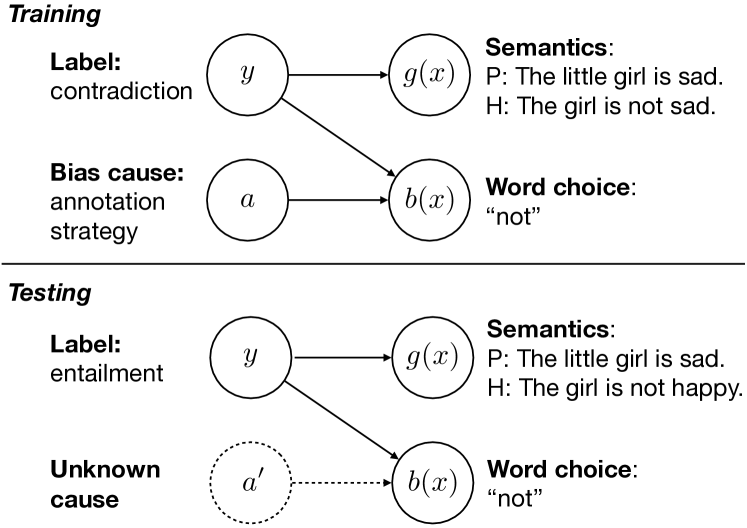
A common problem behind these failures is distribution shift. Our training data is often not a representative sample of real-world data due to their different data-generating processes, thus models are susceptible to learning simple cues (e.g., lexical overlap) that work well on the majority of training examples but fail on more challenging test examples. Consider generating a contradicting pair of sentences for natural language inference (NLI) in Figure 1. Crowd workers tend to mechanically negate the premise sentence to save time, introducing an association between negation words (e.g., “not”) and the contradiction label. However, at test time, such association may not exist as data is now generated by end users. Thus, a model that heavily relies on the biased feature “not” would fail. In this paper, we formalize dataset bias Torralba and Efros (2011) under the label shift assumption: the conditional distribution of the label given biased features changes at test time. Our goal is to design learning algorithms that are robust to dataset bias with a focus on NLI, i.e. predicting whether the premise sentence entails the hypothesis sentence.
Typical debiasing approaches aim to remove biased features (e.g., gender and image texture) in the learned representation Wang et al. (2019b, a). However, biased features in textual data often conflate useful semantic information and superficial cues, thus completely removing them might significantly hurt prediction performance. Even when we are confident that the bias is irrelevant to prediction (e.g., gender), Gonen and Goldberg (2019) show that existing bias removal methods are insufficient.
Instead of debiasing the data representation, our method (along with the concurrent work of Clark et al. (2019)) accounts for label shift given biased features by focusing on “hard” examples that cannot be predicted well using only biased features. We train a model in two steps. First, we train a biased model using insufficient features such as overlapping words between the premise and the hypothesis. Next, we train a debiased model by fitting to the residuals of the biased model. This step “unlearns” the bias by taking additional negative gradient updates on examples with low loss under the biased model (Section 3.2).222 Note that dataset bias is flagged by good performance despite insufficient input, e.g., a high-accuracy hypothesis-only classifier Gururangan et al. (2018). At test time, only the debiased model is used for prediction. We call this learning algorithm DRiFt (Debias by Residual Fitting).
We use DRiFt to train three high-performing NLI models on two benchmark datasets, SNLI Bowman et al. (2015) and MNLI Williams et al. (2017). Compared to baseline models trained by maximum likelihood estimation, our debiased models improve performance on several challenge datasets with only slight degradation on the original test sets.
2 Problem Statement
Dataset bias.
Let be the input and be the label we want to predict. Given training examples drawn from a distribution , we define dataset bias as (partial) representation of that exhibits label shift Lipton et al. (2018); Scholkopf et al. (2012) on the test distribution . Formally, assume that can be represented by two components and conditionally independent given . We have
| (1) | ||||
| (2) |
Let be the true effect of such that their relationship does not change normally, i.e. . Let be biased features that happen to be predictive of on . For example, in Figure 1, represents semantics of the premis and hypothesis sentences, whereas represents specific word choices affected by varying sources. In the training data, the word “not” has a strong association with “contradiction” due to crowd workers’ writing strategies. Consequently, a model learned on the training data distribution would degrade when such association no longer exists. Formally, both training and testing examples may exhibit biased features: , but dependence between these features and the label can change: .
In a typical supervised learning setting with dataset bias, we do not observe examples from thus is unknown. Without additional information, achieving good performance on is impossible. Fortunately, oftentimes we do have domain-specific knowledge on what might be, e.g., the word overlapping heuristic in NLI. Therefore, our goal is to correct the model trained on to perform well on given known dataset bias.
Bias in NLI data.
Dataset bias in SNLI Bowman et al. (2015) and MNLI Williams et al. (2017) are largely due to the crowdsourcing process. Both are created by asking crowd workers to write three sentences (hypotheses) that are entailed by, neutral with, or contradict a given sentence drawn from a corpus (the premise). Gururangan et al. (2018); Poliak et al. (2018) show that certain words in the hypothesis have high pointwise mutual information with class labels regardless of the premise, which could be artifacts of specific annotation strategies. For example, one can create a neutral sentence by adding a cause (“because”) to the premise and create a contradicting sentence by negating (“no”, “never”) the premise. As a result, the majority of training examples can be solved without much reasoning about sentence meanings. Subsequently, McCoy et al. (2019) report that models rely on high word overlap to predict entailment; Glockner et al. (2018); Naik et al. (2018) demonstrate that models struggle at even lexical-level inference involving antonyms, hypernyms, etc.
A natural question to ask then is whether there exist better data collection procedures that guard against these biases. We argue that this is not easy because in practice, we almost always have different data-generating processes during training (generated from selected corpora and annotators) and test (generated by end users). Then, can we remove biased features from training examples? This is also infeasible because sometimes they contain the necessary information for prediction, e.g., removing words may destroy the sentence meaning. It is not the features that are biased but their relation with the label. Next, we describe our approach to mitigating this biased relation.
3 Approach
3.1 Overview
The key idea of our approach is to first detect biased examples given prior knowledge on potential dataset bias, then focus on learning from unbiased, hard examples. We describe the two steps in details below.
Detect biased examples.
How do we know if an example exhibits biased features? Although we cannot directly measure label shift without accessing the test data, we know that NLI models are unlikely to work well given insufficient features. When it does work well given only partial semantics of the input, the good performance is likely due to dataset bias. For example, Gururangan et al. (2018) exposes annotation artifacts by showing that hypothesis-only models have unexpected high accuracy. Similarly, we train a biased classifier using insufficient features , e.g., the hypothesis sentence. We assume that examples predicted well by the biased classifier exhibit dataset bias, i.e. is high but is low.
Importantly, while approximates given our prior knowledge, it does not necessarily capture all dataset bias, which depends on the unknown test distribution. In addition, may include useful information. For example, although bag-of-words (BOW) features are insufficient to represent precise sentence meaning, it encodes a distribution of possible meanings. Thus good performance of a BOW classifier is not fully due to fitting dataset bias. In practice, as we will see in the experiments (Section 4.5), good choices of capture biased features precisely, resulting in significant performance drop of the biased classifier on .
Learn residuals of the biased classifier.
Our intuition is that the debiased classifier should capture information beyond those contained in the biased classifier. If the biased classifier already has a small loss on an example, then there is not much to learn beyond the biased features; otherwise, the debiased classifier should correct predictions of the biased classifier.
We implement the idea through a residual fitting procedure (DRiFt). Let and be the biased and the debiased classifiers, and let be the loss function. First, we learn with insufficient features as the input:
| (3) |
Let be the optimal predictor that minimizes the empirical risk on . We define
| (4) |
Thus fits the residual of with respect to the target . To estimate parameters of , we fix parameters of and minimize the loss:
| (5) |
At test time, we only use the debiased classifier .
Consider the typical empirical risk minimization approach that estimates by minimizing . It is susceptible to relying on biased features when they predict well on the majority examples. In contrast, DRiFt first learns which is intended to fit potential bias in the data. It then learns that compensates without fitting to the bias already captured by it.
Next, we analyze the behavior of DRiFt using the cross-entropy loss function, which is typically used for classification problems.
3.2 Analysis with the Cross-Entropy Loss
In this section, we show that DRiFt adjusts the gradient on each example depending on how well it is predicted by the pretrained biased classifier.
Given the cross-entropy loss, our goal is to maximize the expected conditional log-likelihood of the data, . A classifier outputs a vector of scores for each of the classes, , which are then mapped to a probability distribution by the softmax function. Given classifiers and , we have three choices of parametrization of the conditional probability :
| (6) | ||||
| (7) | ||||
| (8) |
To learn the classifier , standard maximum likelihood estimation (MLE) uses , whereas DRiFt uses given pretrained with fixed parameters.
Let us first compare the two learning objectives. Denote by . DRiFt maximizes
| (9) | ||||
| (10) |
where denotes the training set and is a constant. Compare (10) with the MLE objective:
| (11) |
We see that has an additional regularizer for each example :
| (12) |
Geometrically, it encourages output from the debiased classifier, , to have minimal projection on predicted by the biased classifier.
Next, let’s look at the effect of this regularizer through its gradient. Let be the normalizer . Then, we have
which is derived by writing as . Taking a negative step in the direction of corresponds to down-weighting the probability . Intuitively, the model tries to reweight the output distribution by the gradient weights . Note that
| (13) |
For an example , large values of indicate that is likely to contain biased features. If is also large, the model is probably picking up the bias since has access to complete information in including the biased features, in which case a relatively large negative step is taken to correct it. In the extreme case where the biased classifier makes perfect prediction, we have thus , canceling the MLE gradient . As a result, the gradient on this example is zero, and there is nothing to be learned. At the other end where does not provide any useful information, the biased classifier outputs a uniform distribution , thus and the gradient on this example is reduced to the MLE gradient.
4 Experiments
We first evaluate our method using synthetic bias to show its effectiveness under different amount of dataset bias. We then test on two challenge datasets using different biased classifiers. We show that DRiFt consistently outperforms MLE on the challenge datasets given different NLI models, especially when the insufficient features capture dataset bias exploited by the challenge data.
4.1 Training Data
We evaluate DRiFt on two benchmarking NLI datasets: SNLI Bowman et al. (2015) and MNLI Williams et al. (2017). Each pair of premise and hypothesis sentences has a label from one of “entailment”, “contradiction”, or “neutral”. Sentences from SNLI are derived from image captions, whereas MNLI covers a broader range of styles and topics. Statistics of the two datasets are shown in Table 1. All MNLI results are on the matched development set.333 MNLI has two development sets, one from the same source as the training data (matched) and one from different sources (mismatched). We trained two sets of models using their corresponding development sets for model selection and obtained similar results. Thus we focus on the “matched” results.
| Dataset | Train | Dev | Test |
|---|---|---|---|
| SNLI | 549,367 | 9842 | 9842 |
| MNLI | 392,702 | 9815 | - |
4.2 Models and Training Details
DRiFt is a general learning algorithm that works with any biased/debiased models. Below we describe the three key components of our approaches: the learning algorithm, the biased model with its insufficient features, and the debiased model.
Learning algorithms.
We compare DRiFt with MLE, as well as a simpler variant of DRiFt: instead of the residual fitting, we remove the examples predicted correctly by the biased classifier and train on the rest. We call this baseline Rm, which is also conceived by Gururangan et al. (2018). MLE only trains the debiased model. Both DRiFt and Rm rely on an additional biased model that captures potential dataset bias.
Biased models.
We consider three insufficient representations that exploit various NLI dataset biases reported in prior work.
Hypo
is a finetuned BERT classifier that uses only the hypothesis sentence.
CBOW
is a continuous bag-of-words classifier. Similar to Mou et al. (2016), we represent both the premise and the hypothesis as the respective sums of their word embeddings. We then concatenate the premise and the hypothesis embeddings, their difference, and their element-wise product. The final representation is passed through a one-layer fully connected network with ReLU activation.
Hand
is a classifier using handcrafted features based on error analysis in Naik et al. (2018). Specifically, we include tokens in the hypothesis that are also in the premise, tokens unique to the hypothesis, Jaccard similarity between the two sentences, whether negation words (“not” and “n’t”) are included, and length difference computed by where and are numbers of tokens in the premise and the hypothesis. We represent the overlapping and the non-overlapping tokens as the respective sums of their word embeddings. The embeddings are then concatenated with the dense features and passed through a one-layer fully connected network with ReLU activation.
Debiased models.
We choose three high-performing models of different capability.
DA
is the Decomposable Attention model introduced by Parikh et al. (2016), which relies on the interaction between words in the premise and the hypothesis. It does not use any word order information. We used the variant without intra-sentence attention.444 We removed the projection layers of the word embeddings as it speeds up training without hurting performance in our experiments.
ESIM
is the Enhanced Sequential Inference Model Chen et al. (2017). It first encodes the premise and the hypothesis by a bidirectional LSTM, aligns the contextual word embeddings similar to Parikh et al. (2016), and uses another “inference” bidirectional LSTM to aggregate information. Thus it has access to the non-local context.
BERT
is the Bidirectional Encoder Representations from Transformers Devlin et al. (2019) that recently improved performance on MNLI significantly. It uses contextual embeddings pretrained from large corpora.
Hyperparameters.
For non-BERT models, word embeddings are initialized with the 840B.300d pretrained GloVe Pennington et al. (2014) word vectors and finetuned during training. For DA and ESIM, hyperparameters of the model architecture are the same as those reported in the original papers. We finetune all BERT models from the pretrained BERT-base-uncased model.555 http://gluon-nlp.mxnet.io/model_zoo/bert/index.html We train all models using the Adam Kingma and Ba (2014) optimizer with , , L2 weight decay of 0.01, learning rate warmup for the first of updates and linear decay afterwards. We use a dropout rate of 0.1 for all models except ESIM, which has a dropout rate of 0.5. BERT and non-BERT models are trained with a learning rate of 2e-5 and 1e-4, respectively. For MLE, we train BERT for 4 epochs and the rest for 30 epochs. When training the debiased model in DRiFt, we find that the models converge slowly thus we train BERT for 8 epochs and the rest for 80 epochs.
4.3 In-Distribution Performance
We first evaluate the models’ in-distribution performance where they are trained and evaluated on splits from the same dataset. Results of the biased models are reported in Table 2. All exceeds the majority-class baseline by a large margin, indicating that a majority of examples can be solved by superficial cues.
Results of the debiased models are reported in Table 3. Baseline results from our implementations are comparable to prior reported performance (row “MLE”). Debiased models trained by DRiFt show some degradation on in-distribution data, especially for the less powerful DA and ESIM models. The accuracy drop is expected due to two reasons. First, DRiFt assumes distribution shift thus does not optimize performance on the training distribution . Second, the effective training data size is reduced by negative gradients on potentially biased examples; this effect is exaggerated by Rm, which shows significant in-distribution degradation. Similar trade-off between in-distribution accuracy and robustness on out-of-distribution data has also been observed in adversarial training Zhang et al. (2019b); Tsipras et al. (2019).
| Dataset | majority | Hypo | CBOW | Hand |
|---|---|---|---|---|
| SNLI | 34.2 | 61.8 | 81.2 | 76.7 |
| MNLI | 35.4 | 52.5 | 66.1 | 65.4 |
| SNLI | MNLI | |||||
| BERT | DA | ESIM | BERT | DA | ESIM | |
| MLE | 90.8 | 85.3 | 88.0 | 84.5 | 72.2 | 78.1 |
| DRiFt-Hypo | 89.8 | 83.9 | 86.3 | 84.3 | 68.6 | 75.0 |
| DRiFt-CBOW | 84.7 | 62.6 | 62.3 | 82.1 | 56.3 | 68.8 |
| DRiFt-Hand | 86.5 | 75.0 | 79.2 | 81.7 | 58.8 | 68.9 |
| Rm-Hypo | 71.2 | 67.0 | 70.3 | 65.5 | 57.5 | 63.0 |
| Rm-CBOW | 35.8 | 27.1 | 22.2 | 54.9 | 26.8 | 27.1 |
| Rm-Hand | 46.3 | 37.2 | 38.1 | 51.7 | 34.6 | 37.4 |
4.4 Synthetic Bias
In this section, we evaluate our model under controlled, synthetic dataset bias on SNLI. Recall our definition of dataset bias: the conditional distribution of the label given biased features are different on training and test sets. Therefore, we inject bias into each example by adding a cheating feature that encodes its label. On training and development examples, the cheating feature encodes the ground truth label with probability (the cheating rate), and a random label otherwise. On test examples, the cheating feature always encodes a random label. Thus a model relying on the cheating feature would perform poorly on the test set.
Specifically, we prepend the hypothesis with a string “{label} and” where . To simulate the fact that we often cannot pinpoint biased features until the model fails on some test examples, we choose Hypo as our biased classifier. That is to say, we have a rough idea that the bias might be in the hypothesis but do not know what it is exactly.
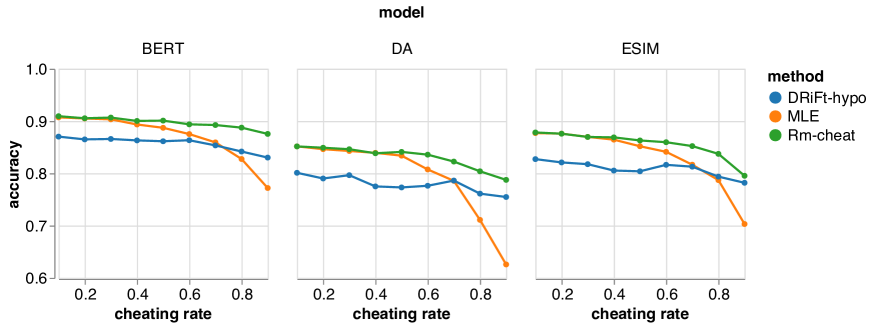
We train all three base models (DA, ESIM, and BERT) using MLE and DRiFt, respectively. Our results are shown in Figure 2. All MLE models are reasonably robust to a mild amount of bias. However, when a majority () of training examples contains the bias, their accuracy decreases significantly: about drop at compared to the baseline accuracy when no cheating features are injected. BERT is slightly more robust than DA and ESIM, possibly due to the regularization effect of pretrained embeddings. In contrast, our debiased models (DRiFt-Hypo) maintain similar accuracies with increasing cheating rates and have a maximum accuracy drop of about .
Two questions remain, though: (1) Why does the accuracy of debiased models still drop a bit at high cheating rates? (2) Why is the baseline accuracy of DRiFt lower than MLE? We answer these questions by analyzing the upper bound performance of our method below.
Best-case scenario.
In the ideal case, we know precisely what the bias is. Consider a biased classifier that only uses the cheating feature as its input. It predicts biased examples perfectly, i.e. and , and predicts the rest unbiased examples uniformly at random. Based on our discussion at the end of Section 3.2, the biased examples have zero gradients and unbiased examples have the same gradients as in MLE. In this case, our method is equivalent to removing biased examples and training a classifier on the rest, i.e. Rm-cheat. In Figure 2, we see that it completely dominates MLE. The accuracy of Rm-cheat still drops when is large, because there are fewer “good” examples to learn from, not due to fitting the bias. Similarly, DRiFt-Hypo has lower overall accuracy compared to Rm-cheat, because Hypo captures additional (unbiased) features that cannot be fully learned by the debiased model.
Worst-case scenario.
In the extreme case when , all models’ predictions on the test set are random guesses. For MLE, the biased features are no longer differentiable from the generalizable ones, thus there is no reason not to use them. For DRiFt, since the biased model achieves perfect prediction on all training examples, the debiased model receives zero gradient. Therefore, when strong bias presents on all examples, we need more information to correct the bias, e.g., collecting additional data or augmenting examples.
| method | lexical | subseq | const | |||
|---|---|---|---|---|---|---|
| Hypo | 52.6 | 44.4 | 54.5 | 44.3 | 45.6 | 16.7 |
| CBOW | 63.2 | 16.0 | 66.2 | 33.7 | 63.2 | 38.5 |
| Hand | 66.7 | 0.0 | 66.7 | 0.0 | 66.7 | 0.0 |
| model: BERT | ||||||
| MLE | 67.2 | 7.8 | 66.7 | 0.4 | 68.1 | 11.9 |
| DRiFt-Hypo | 84.7 | 79.8 | 69.0 | 23.7 | 72.7 | 40.8 |
| DRiFt-CBOW | 80.8 | 75.2 | 68.5 | 29.5 | 71.5 | 40.3 |
| DRiFt-Hand | 77.4 | 70.9 | 71.2 | 41.2 | 75.8 | 61.0 |
| Rm-Hypo | 67.2 | 46.0 | 65.2 | 36.6 | 75.5 | 72.2 |
| Rm-CBOW | 5.4 | 66.4 | 8.5 | 64.2 | 34.8 | 65.3 |
| Rm-Hand | 10.0 | 66.0 | 4.7 | 66.3 | 9.1 | 67.3 |
| model: DA | ||||||
| MLE | 66.6 | 0.5 | 66.6 | 0.3 | 66.5 | 0.4 |
| DRiFt-Hypo | 66.3 | 1.7 | 66.9 | 5.5 | 66.3 | 8.4 |
| DRiFt-CBOW | 65.3 | 7.2 | 66.1 | 9.6 | 65.1 | 9.1 |
| DRiFt-Hand | 60.5 | 27.1 | 61.4 | 44.9 | 55.9 | 48.3 |
| Rm-Hypo | 65.1 | 9.6 | 66.2 | 15.0 | 66.2 | 18.8 |
| Rm-CBOW | 0.4 | 66.6 | 1.3 | 66.7 | 0.8 | 66.5 |
| Rm-Hand | 10.3 | 65.8 | 8.9 | 65.7 | 13.9 | 64.7 |
| model: ESIM | ||||||
| MLE | 65.8 | 3.2 | 67.2 | 4.6 | 65.5 | 2.8 |
| DRiFt-Hypo | 64.3 | 10.5 | 68.3 | 16.3 | 68.1 | 29.3 |
| DRiFt-CBOW | 63.2 | 14.4 | 66.8 | 20.1 | 64.9 | 22.7 |
| DRiFt-Hand | 61.2 | 19.6 | 63.7 | 39.4 | 64.8 | 48.3 |
| Rm-Hypo | 63.3 | 12.8 | 64.1 | 24.8 | 71.3 | 46.0 |
| Rm-CBOW | 4.5 | 65.7 | 6.0 | 65.2 | 16.9 | 63.8 |
| Rm-Hand | 25.8 | 60.8 | 18.3 | 67.3 | 13.1 | 65.9 |
4.5 Word Overlap Bias
We evaluate our method on word overlap bias in NLI. McCoy et al. (2019) show that models trained on MNLI largely rely on word overlap between the premise and the hypothesis to make entailment predictions. They created a challenge dataset (HANS) where premises may not entail high word-overlapping hypotheses. Specifically, a model biased by word overlap would fail on three types of non-entailment examples: (1) Lexical overlap, e.g., “The doctor visited the lawyer.” “The lawyer visited the doctor.”. (2) Subsequence, e.g., “The senator near the lawyer danced.” “The lawyer danced.”. (3) Constituent, e.g., “The lawyers resigned, or the artist slept.” “The artist slept.”.
We evaluate both biased and debiased models on the three subsets of HANS and show F1 scores for each class in Table 4. As expected, models trained by MLE almost always predict entailment (), and thus performs poorly for the non-entailment class (). DRiFt improves performance on in all cases with little degradation on . In contrast, Rm improves performance on at the cost of significant degradation on .
Among all biased models, Hand produces the best debiasing results because it is designed to fit the word overlap bias, and indeed has zero recall on when tested on HANS. On the contrary, the improvement from Hypo is lower because it does not capture any word overlap bias. Correspondingly, its performance drop on HANS is minimal compared to its in-distribution performance. Among all debiased models, BERT has the best overall performance. We hypothesize that pretraining on large data improves model robustness in addition to the debiasing effect from DRiFt.
4.6 Stress Tests
| method | Negation | Overlap | ||||
|---|---|---|---|---|---|---|
| Hypo | 41.2 | 52.4 | 50.5 | 44.2 | 52.8 | 51.7 |
| CBOW | 20.1 | 48.2 | 53.9 | 49.7 | 52.9 | 55.6 |
| Hand | 37.5 | 45.0 | 57.3 | 56.7 | 50.1 | 57.8 |
| model: BERT | ||||||
| MLE | 2.4 | 81.1 | 56.5 | 19.2 | 83.3 | 59.4 |
| DRiFt-Hypo | 7.3 | 80.7 | 55.6 | 27.5 | 81.1 | 59.1 |
| DRiFt-CBOW | 17.9 | 81.7 | 55.5 | 18.3 | 80.0 | 56.6 |
| DRiFt-Hand | 4.3 | 80.6 | 55.5 | 15.0 | 81.9 | 57.4 |
| model: DA | ||||||
| MLE | 17.4 | 47.3 | 55.3 | 46.7 | 60.5 | 57.8 |
| DRiFt-Hypo | 11.8 | 47.0 | 51.8 | 41.6 | 59.4 | 55.6 |
| DRiFt-CBOW | 28.4 | 21.4 | 39.5 | 35.2 | 41.7 | 43.8 |
| DRiFt-Hand | 24.7 | 42.0 | 46.4 | 42.2 | 56.0 | 49.9 |
| model: ESIM | ||||||
| MLE | 12.0 | 72.7 | 54.6 | 27.6 | 76.4 | 57.5 |
| DRiFt-Hypo | 22.8 | 67.7 | 54.0 | 37.5 | 73.2 | 56.7 |
| DRiFt-CBOW | 32.7 | 62.3 | 46.9 | 30.4 | 65.6 | 49.8 |
| DRiFt-Hand | 15.8 | 64.6 | 51.8 | 39.2 | 70.7 | 53.9 |
In addition to the word overlap bias exploited by HANS, there are other known biases such as negation words and sentence lengths. Naik et al. (2018) conduct a detailed error anlaysis on MNLI and create six stress test sets (Stress) targeting at each type of error. We focus on the word overlap and negation stress test sets, which expose dataset bias as opposed to model weakness according to Liu et al. (2019). A model biased by word overlap rate and negation words are expected to have low accuracy on the entailment class on challenge data. The complete results are shown in Appendix A.
In Table 5, we show the F1 scores of each class for all models on Stress.666 Since results of Rm are similar to those in Table 4, we put them in Appendix A. Compared to results on HANS, Stress sees lower overall improvement from debiasing. One reason is that Stress decreases word overlap rate and injects negation words by appending distractor phrases, i.e. “true is true” and “false is not true”. While this introduces label shift on biased features, it also introduces covariate shift on the input. For example, although Hand contains features designed to use word overlap rate (Jaccard similarity) and negation words, its does not have big performance drop on the challenge data compared to its in-distribution performance, showing that that distractor phrases may affect the model in other ways.
While all debiased models show improvement on , both DA and ESIM suffer from degradation on the other two classes, especially when trained by DRiFt-CBOW. We posit two reasons. First, while CBOW is insufficient to represent complete sentence meaning, it does encode a distribution of possible meanings. Thus models debiased by DRiFt-CBOW might discard useful information. Second, model capacity limits what is learned beyond a BOW representation. DA shows the most degradation since it only uses local word interaction, thus is essentially a BOW model. In contrast, BERT has little degradation on in-distribution examples regardless of the biased classifier.
5 Related Work and Discussion
Adversarial data collection.
Aside from NLI, dataset bias has been exposed on benchmarks for other NLP tasks as well, e.g., paraphrase identification (Zhang et al., 2019c, a), story close test Schwartz et al. (2017), reading comprehension Kaushik and Lipton (2018), coreference resolution Zhao et al. (2018a), and visual question answering Agrawal et al. (2016). Most bias is resulted from artifacts in the data selection procedure and shortcuts taken by crowd workers. To systematically minimize bias during data collection, adversarial filtering methods Sakaguchi et al. (2019); Zellers et al. (2019) have been proposed to discard examples predicted well by a simple classifier. This is similar to the Rm baseline, except that we apply “filtering” at training time. In general, our debiasing methods are complementary to adversarial data collection methods.
Debiased representation.
Our work is closely related to the line of work on removing bias in data representations. Bolukbasi et al. (2016); Zhao et al. (2018b) learn gender-neutral word embeddings by forcing certain dimensions to be free of gender information. Similarly, Wang et al. (2019a) construct a biased classifier and project its representation out of the model’s representation. For NLI, Belinkov et al. (2019) use adversarial learning to remove hypothesis-related bias in the sentence representations. However, for some NLP applications it may not be easy to separate biased features from useful semantic representations, thus we correct the conditional distribution of the class label given these biased features instead of removing them from the input. Concurrently, Clark et al. (2019) take the same approach and further show its effectiveness on additional tasks including reading comparehension and visual question answering.
Distribution shift.
Covariate shift Shimodaira (2000); Ben-David et al. (2006) and label shift Lipton et al. (2018); Zhang et al. (2013) are two well-studied settings under distribution shift, which makes different assumptions on how changes. However, most works in these settings assume access to unlabeled data from the target distribution. Our objective is more related to distributionally robust optimization Duchi and Namkoong (2018); Hu et al. (2018), which does not assume access to target data and optimizes the worst-case performance under unknown, bounded distribution shift. In contrast, we leverage prior knowledge on potential dataset bias.
Data augmentation.
An effective way to tackle the challenge datasets is to train or finetune on similar examples McCoy et al. (2019); Liu et al. (2019); Jia and Liang (2017), which explicitly correct the training data distribution. However, constructing challenge examples often rely on handcrafted rules that target a specific type of bias, e.g., swapping male and female entities Zhao et al. (2018a, 2019), synonym/antonym substitution Glockner et al. (2018), and syntactic rules McCoy et al. (2019); Ribeiro et al. (2018), and may require human verification Zhang et al. (2019c); Jia and Liang (2017). Data augmentation provides a way to encode our prior knowledge on the task, e.g., swapping genders does not affect coreference resolution result, and syntactic transformations may affect sentence meanings. Therefore, a related direction is to develop generic augmentation techniques with linguistic priors Andreas (2019); Karpukhin et al. (2019).
6 Conclusion
Across all different dataset biases, the fundamental problem is that the majority training examples are not representative of the real-world data distribution (including the challenge data), thus minimizing the average training loss no longer accurately describes our objective. In this paper, we tackle the problem by adapting the learning objective to focus on examples that cannot be easily solved by biased features. We show that our debiasing method improves model performance on challenge data given known dataset bias. However, current improvements largely rely on task-specific prior knowledge, thus an important next step is to develop more general methods that tackle different types of biases.
Acknowledgments
Yanchao Ni worked on an earlier version of this project while he was at New York University. We thank the GluonNLP community for their support on reproducing prior results.
References
- Agrawal et al. (2016) A. Agrawal, D. Batra, and D. Parikh. 2016. Analyzing the behavior of visual question answering models. In Empirical Methods in Natural Language Processing (EMNLP).
- Andreas (2019) J. Andreas. 2019. Good-enough compositional data augmentation. arXiv.
- Belinkov et al. (2019) Y. Belinkov, A. Poliak, S. M. Shieber, B. V. Durme, and A. M. Rush. 2019. Don’t take the premise for granted: Mitigating artifacts in natural language inference. In Association for Computational Linguistics (ACL).
- Ben-David et al. (2006) S. Ben-David, J. Blitzer, K. Crammer, and F. Pereira. 2006. Analysis of representations for domain adaptation. In Advances in Neural Information Processing Systems (NeurIPS), pages 137–144.
- Bolukbasi et al. (2016) T. Bolukbasi, K. Chang, J. Y. Zou, V. Saligrama, and A. T. Kalai. 2016. Man is to computer programmer as woman is to homemaker? debiasing word embeddings. In Advances in Neural Information Processing Systems (NeurIPS), pages 4349–4357.
- Bowman et al. (2015) S. Bowman, G. Angeli, C. Potts, and C. D. Manning. 2015. A large annotated corpus for learning natural language inference. In Empirical Methods in Natural Language Processing (EMNLP).
- Chen et al. (2017) Q. Chen, X. Zhu, Z. Ling, S. Wei, H. Jiang, and D. Inkpen. 2017. Enhanced LSTM for natural language inference. In Association for Computational Linguistics (ACL).
- Clark et al. (2019) C. Clark, M. Yatskar, and L. Zettlemoyer. 2019. Don’t take the easy way out: Ensemble based methods for avoiding known dataset biases. In Empirical Methods in Natural Language Processing (EMNLP).
- Devlin et al. (2019) J. Devlin, M. Chang, K. Lee, and K. Toutanova. 2019. Bert: Pre-training of deep bidirectional transformers for language understanding. In North American Association for Computational Linguistics (NAACL).
- Duchi and Namkoong (2018) J. Duchi and H. Namkoong. 2018. Learning models with uniform performance via distributionally robust optimization. arXiv preprint arXiv:1810.08750.
- Glockner et al. (2018) M. Glockner, V. Shwartz, and Y. Goldberg. 2018. Breaking NLI systems with sentences that require simple lexical inferences. In Association for Computational Linguistics (ACL).
- Gonen and Goldberg (2019) H. Gonen and Y. Goldberg. 2019. Lipstick on a pig: Debiasing methods cover up systematic gender biases in word embeddings but do not remove them. arXiv preprint arXiv:1903.03862.
- Gururangan et al. (2018) S. Gururangan, S. Swayamdipta, O. Levy, R. Schwartz, S. R. Bowman, and N. A. Smith. 2018. Annotation artifacts in natural language inference data. In North American Association for Computational Linguistics (NAACL).
- Hu et al. (2018) W. Hu, G. Niu, I. Sato, and M. Sugiyama. 2018. Does distributionally robust supervised learning give robust classifiers? In International Conference on Machine Learning (ICML).
- Jia and Liang (2017) R. Jia and P. Liang. 2017. Adversarial examples for evaluating reading comprehension systems. In Empirical Methods in Natural Language Processing (EMNLP).
- Karpukhin et al. (2019) V. Karpukhin, O. Levy, J. Eisenstein, and M. Ghazvininejad. 2019. Training on synthetic noise improves robustness to natural noise in machine translation. arXiv.
- Kaushik and Lipton (2018) D. Kaushik and Z. C. Lipton. 2018. How much reading does reading comprehension require? a critical investigation of popular benchmarks. In Empirical Methods in Natural Language Processing (EMNLP).
- Kingma and Ba (2014) D. Kingma and J. Ba. 2014. Adam: A method for stochastic optimization. arXiv preprint arXiv:1412.6980.
- Lipton et al. (2018) Z. C. Lipton, Y. Wang, and A. J. Smola. 2018. Detecting and correcting for label shift with black box predictors. In International Conference on Machine Learning (ICML).
- Liu et al. (2019) N. F. Liu, R. Schwartz, and N. A. Smith. 2019. Inoculation by fine-tuning: A method for analyzing challenge datasets. In North American Association for Computational Linguistics (NAACL).
- McCoy et al. (2019) R. T. McCoy, E. Pavlick, and T. Linzen. 2019. Right for the wrong reasons: Diagnosing syntactic heuristics in natural language inference. arXiv preprint arXiv:1902.01007.
- Mou et al. (2016) L. Mou, R. Men, G. Li, Y. Xu, L. Zhang, R. Yan, and Z. Jin. 2016. Natural language inference by tree-based convolution and heuristic matching. In Association for Computational Linguistics (ACL).
- Naik et al. (2018) A. Naik, A. Ravichander, N. Sadeh, C. Rose, and G. Neubig. 2018. Stress test evaluation for natural language inference. In International Conference on Computational Linguistics (COLING).
- Parikh et al. (2016) A. Parikh, O. Täckström, D. Das, and J. Uszkoreit. 2016. A decomposable attention model for natural language inference. In Empirical Methods in Natural Language Processing (EMNLP).
- Pennington et al. (2014) J. Pennington, R. Socher, and C. D. Manning. 2014. GloVe: Global vectors for word representation. In Empirical Methods in Natural Language Processing (EMNLP), pages 1532–1543.
- Poliak et al. (2018) A. Poliak, J. Naradowsky, A. Haldar, R. Rudinger, and B. V. Durme. 2018. Hypothesis only baselines in natural language inference. arXiv preprint arXiv:1805.01042.
- Ribeiro et al. (2018) M. T. Ribeiro, S. Singh, and C. Guestrin. 2018. Semantically equivalent adversarial rules for debugging NLP models. In Association for Computational Linguistics (ACL).
- Sakaguchi et al. (2019) K. Sakaguchi, R. L. Bras, C. Bhagavatula, and Y. Choi. 2019. WINOGRANDE: An adversarial winograd schema challenge at scale. arXiv preprint arXiv:1907.10641.
- Scholkopf et al. (2012) B. Scholkopf, D. Janzing, J. Peters, E. Sgouritsa, K. Zhang, and J. Mooij. 2012. On causal and anticausal learning. In International Conference on Machine Learning (ICML).
- Schwartz et al. (2017) R. Schwartz, M. Sap, Y. Konstas, L. Zilles, Y. Choi, and N. A. Smith. 2017. The effect of different writing tasks on linguistic style: A case study of the ROC story cloze task. In Computational Natural Language Learning (CoNLL).
- Shimodaira (2000) H. Shimodaira. 2000. Improving predictive inference under covariate shift by weighting the log-likelihood function. Journal of Statistical Planning and Inference, 90:227–244.
- Torralba and Efros (2011) A. Torralba and A. Efros. 2011. Unbiased look at dataset bias. In Computer Vision and Pattern Recognition (CVPR).
- Tsipras et al. (2019) D. Tsipras, S. Santurkar, L. Engstrom, A. Turner, and A. Madry. 2019. Robustness may be at odds with accuracy. In International Conference on Learning Representations (ICLR).
- Wang et al. (2019a) H. Wang, Z. He, Z. C. Lipton, and E. P. Xing. 2019a. Learning robust representations by projecting superficial statistics out. In International Conference on Learning Representations (ICLR).
- Wang et al. (2019b) T. Wang, J. Zhao, M. Yatskar, K. Chang, and V. Ordonez. 2019b. Balanced datasets are not enough: Estimating and mitigating gender bias in deep image representations. In International Conference on Computer Vision (ICCV).
- Williams et al. (2017) A. Williams, N. Nangia, and S. R. Bowman. 2017. A broad-coverage challenge corpus for sentence understanding through inference. arXiv preprint arXiv:1704.05426.
- Zellers et al. (2019) R. Zellers, A. Holtzman, Y. Bisk, A. Farhadi, and Y. Choi. 2019. HellaSwag: Can a machine really finish your sentence? In Association for Computational Linguistics (ACL).
- Zhang et al. (2019a) G. Zhang, B. Bai, J. Liang, K. Bai, S. Chang, M. Yu, C. Zhu, and T. Zhao. 2019a. Selection bias explorations and debias methods for natural language sentence matching datasets. In Association for Computational Linguistics (ACL).
- Zhang et al. (2019b) H. Zhang, Y. Yu, J. Jiao, E. P. Xing, L. E. Ghaoui, and M. I. Jordan. 2019b. Theoretically principled trade-off between robustness and accuracy. arXiv preprint arXiv:1901.08573.
- Zhang et al. (2013) K. Zhang, B. Schölkopf, K. Muandet, and Z. Wang. 2013. Domain adaptation under target and conditional shift. In International Conference on Machine Learning (ICML).
- Zhang et al. (2019c) Y. Zhang, J. Baldridge, and L. He. 2019c. PAWS: Paraphrase adversaries from word scrambling. In North American Association for Computational Linguistics (NAACL).
- Zhao et al. (2019) J. Zhao, T. Wang, M. Yatskar, R. Cotterell, V. Ordonez, and K. Chang. 2019. Gender bias in contextualized word embeddings. In North American Association for Computational Linguistics (NAACL).
- Zhao et al. (2018a) J. Zhao, T. Wang, M. Yatskar, V. Ordonez, and K. Chang. 2018a. Gender bias in coreference resolution:evaluation and debiasing methods. In North American Association for Computational Linguistics (NAACL).
- Zhao et al. (2018b) J. Zhao, Y. Zhou, Z. Li, W. Wang, and K. Chang. 2018b. Learning gender-neutral word embeddings. In Empirical Methods in Natural Language Processing (EMNLP).
| Negation | Overlap | Antonym | Length | ||||||||||
| Hypo | MLE | 41.2 | 52.4 | 50.5 | 44.2 | 52.8 | 51.7 | - | 40.5 | - | 55.1 | 52.5 | 51.5 |
| CBOW | 20.1 | 48.2 | 53.9 | 49.7 | 52.9 | 55.6 | - | 19.0 | - | 21.9 | 55.5 | 49.4 | |
| Hand | 37.5 | 45.0 | 57.3 | 56.7 | 50.1 | 57.8 | - | 28.2 | - | 66.6 | 65.0 | 60.7 | |
| BERT | MLE | 2.4 | 81.1 | 56.5 | 19.2 | 83.3 | 59.4 | - | 66.0 | - | 83.8 | 83.6 | 77.4 |
| DRiFt-Hypo | 7.3 | 80.7 | 55.6 | 27.5 | 81.1 | 59.1 | - | 75.4 | - | 84.1 | 83.2 | 76.3 | |
| DRiFt-CBOW | 17.9 | 81.7 | 55.5 | 18.3 | 80.0 | 56.6 | - | 75.3 | - | 82.4 | 82.3 | 74.6 | |
| DRiFt-Hand | 4.3 | 80.6 | 55.5 | 15.0 | 81.9 | 57.4 | - | 76.0 | - | 81.4 | 82.5 | 74.9 | |
| Rm-Hypo | 32.1 | 55.9 | 39.9 | 44.4 | 63.8 | 43.0 | - | 69.3 | - | 72.9 | 70.9 | 52.4 | |
| Rm-CBOW | 33.6 | 61.6 | 42.7 | 29.4 | 65.2 | 44.7 | - | 85.1 | - | 69.7 | 60.8 | 55.7 | |
| Rm-Hand | 20.7 | 49.7 | 40.0 | 30.9 | 54.7 | 39.6 | - | 83.8 | - | 57.2 | 52.6 | 46.5 | |
| DA | MLE | 17.4 | 47.3 | 55.3 | 46.7 | 60.5 | 57.8 | - | 59.8 | - | 69.5 | 66.0 | 61.9 |
| DRiFt-Hypo | 11.8 | 47.0 | 51.8 | 41.6 | 59.4 | 55.6 | - | 57.4 | - | 66.4 | 63.7 | 55.3 | |
| DRiFt-CBOW | 28.4 | 21.4 | 39.5 | 35.2 | 41.7 | 43.8 | - | 57.8 | - | 64.3 | 39.4 | 53.9 | |
| DRiFt-Hand | 24.7 | 42.0 | 46.4 | 42.2 | 56.0 | 49.9 | - | 72.4 | - | 48.4 | 57.6 | 51.2 | |
| Rm-Hypo | 14.9 | 39.9 | 45.3 | 52.0 | 52.6 | 46.0 | - | 56.6 | - | 63.9 | 62.2 | 32.0 | |
| Rm-CBOW | 3.8 | 23.9 | 38.0 | 2.6 | 17.1 | 41.5 | - | 53.1 | - | 4.4 | 33.5 | 29.9 | |
| Rm-Hand | 31.6 | 26.4 | 36.2 | 40.6 | 37.6 | 29.6 | - | 57.8 | - | 40.0 | 27.6 | 33.1 | |
| ESIM | MLE | 12.0 | 72.7 | 54.6 | 27.6 | 76.4 | 57.5 | - | 75.1 | - | 77.6 | 76.8 | 68.8 |
| DRiFt-Hypo | 22.8 | 67.7 | 54.0 | 37.5 | 73.2 | 56.7 | - | 75.5 | - | 75.9 | 74.3 | 66.3 | |
| DRiFt-CBOW | 32.7 | 62.3 | 46.9 | 30.4 | 65.6 | 49.8 | - | 67.0 | - | 68.5 | 60.2 | 60.1 | |
| DRiFt-Hand | 15.8 | 64.6 | 51.8 | 39.2 | 70.7 | 53.9 | - | 74.7 | - | 68.8 | 70.9 | 61.6 | |
| Rm-Hypo | 29.6 | 54.4 | 45.3 | 47.3 | 63.6 | 46.1 | - | 60.4 | - | 70.6 | 68.2 | 31.1 | |
| Rm-CBOW | 31.8 | 32.0 | 28.9 | 18.1 | 33.2 | 32.7 | - | 68.3 | - | 26.6 | 18.0 | 40.8 | |
| Rm-Hand | 26.0 | 35.1 | 40.7 | 29.2 | 43.3 | 34.0 | - | 57.4 | - | 31.4 | 35.0 | 35.3 | |
Appendix A Results on MNLI Stress Test
In Table 6, we show the complete results on MNLI Stress Test Naik et al. (2018). In addition to Overlap and Negation, which is intended to test dataset bias, we also include two tests that evaluate model performance on minority examples. Our debiased models have some improvement on Antonym, possibly as a by-product of focusing on challenge examples that cannot be solved by superficial cues. However, DRiFt did not improve performance on Length.