DDSketch: A Fast and Fully-Mergeable Quantile Sketch with Relative-Error Guarantees

Abstract

Summary statistics such as the mean and variance are easily maintained for large, distributed data streams, but order statistics (i.e., sample quantiles) can only be approximately summarized. There is extensive literature on maintaining quantile sketches where the emphasis has been on bounding the rank error of the sketch while using little memory. Unfortunately, rank error guarantees do not preclude arbitrarily large relative errors, and this often occurs in practice when the data is heavily skewed.

Given the distributed nature of contemporary large-scale systems, another crucial property for quantile sketches is mergeablility, i.e., several combined sketches must be as accurate as a single sketch of the same data. We present the first fully-mergeable, relative-error quantile sketching algorithm with formal guarantees. The sketch is extremely fast and accurate, and is currently being used by Datadog at a wide-scale.

1 Introduction

Computing has increasingly moved to a distributed, containerized, micro-service model. Some organizations run thousands of hosts, across several data centers, with each host running a dozen containers each, and these containers might only live for a couple hours [11, 10]. Effectively being able to administer and operationalize such a large and disparate fleet of machines requires the ability to monitor, in near real-time, data streams coming from multiple, possibly transitory, sources [3].

The data streams that are being monitored can include application logs, IoT sensor readings [28], IP-network traffic information [9], financial data, distributed application traces [30], usage and performance metrics [1], along with a myriad of other measurements and events. The volume of monitoring data being transmitted to a central processing system (usually backed by a time-series database or an event storage system) can be high enough that simply forwarding all this information can strain the capacities (network, memory, CPU) of the monitored resources. Ideally a monitoring system helps one discover and diagnose issues in distributed systems—not cause them.

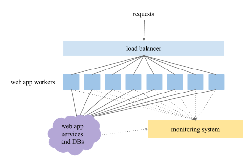
Figure 1: A distributed web application, with each container sending metrics to the monitoring system.

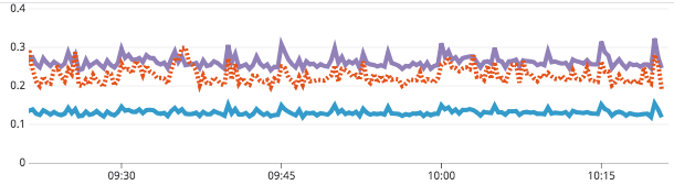
Figure 2: The average latency of a web endpoint over time (dotted line) is closer to the 75th percentile than it is to the 50th (the two solid lines).

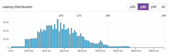
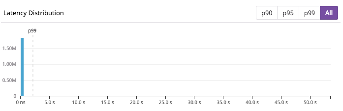
Figure 3: Histograms for p0-p95 and p0-p100 of 2 million web request response times. (Bars for p93-p100 exist but are shorter than the minimum pixel height.)

Our running example will be a web application backed by a distributed system, where the ability to answer any particular request might depend on several underlying services and databases (Figure 1). The metric we monitor for our example will be the latency of the requests it handles. Every time a worker finishes handling a request, it will note how long it took. Simple summary statistics such as the overall mean and variance can be easily maintained. For instance, the workers can keep counts, sums, and sums of squares of the latency and send those values to the monitoring system (and reset those values) every second. The monitoring system will then be able to aggregate those values and derive metrics—being able to graph the average latency using 1 second intervals, but also rolling up the sums and counts to graph the average latency over much larger time periods using much larger intervals perfectly accurately.

Unfortunately, the latencies of web requests are usually extremely skewed—the median response time might be in the milliseconds whereas there could be a couple of outlying responses that take minutes (Figure 3). A simple average, while easy to monitor can be easily skewed by outlying values as can be seen in Figure 2.

As the average response time is not a particularly useful measure, we are instead interested in tracking quantiles such as the 50th and the 99th percentiles (we will also refer to these as the p50 and p99). The ability to compute quantiles over aggregated metrics has been recognized to be an essential feature of any monitoring system [16].

Quantiles are famously impossible to compute exactly without holding on to all the data [29]. If one wanted to track the median request latency over time for a web application that is handling millions of requests a second, this would mean sending millions of data points to the monitoring service which could then calculate the median by sorting the data. If one wanted the median aggregated over longer time intervals the monitoring service would have to store all these data points and then calculate the median over the larger set of points.

Given how expensive calculating exact quantiles can be for both storage and network bandwidth, most monitoring systems will compress the data into sketches and compute approximate quantiles. More formally, given a multiset $S$ of size $n$ over $\mathbb{R}$, the $q$-quantile item $x_{q}\in S$ is the item $x$ whose rank $R(x)$ in the sorted multiset $S$ is ${\lfloor{1+q(n-1)}\rfloor}$ for $0\leq q\leq 1$, where the rank $R(x)$ is the number of elements in $S$ smaller than or equal to $x$. Some special quantiles include $x_{1}$, the maximum element of $S$, and the median $x_{0.5}$. There has been a long line of work on sketching data streams so that the rank accuracy is preserved, i.e., for any value $v$, the sketch provides an estimate rank $\tilde{R}$ such that $|\tilde{R}(v)-R(v)|\leq\epsilon n$ (see [27] and [21] for excellent surveys on much of this work as well as additional motivation for sketching quantiles).

Unfortunately, for data sets with heavy tails, rank-error guarantees can return values with large relative errors. Consider again the histogram of 2M request response times in Figure 3. If we have a quantile sketch with a rank accuracy of 0.005, and ask for the 99th percentile, we are guaranteed to get a value between the 98.5th and 99.5th percentile. In this case this is anywhere from 2 to 20 seconds, which from an end-user’s perspective is the difference between an annoying delay and giving up on the request.

Given the inadequacy of rank accuracy for tracking the higher order quantiles for distributions with heavy tails, we turn instead to relative accuracy.

Definition 1

$\tilde{x}_{q}$ is an $\alpha$-accurate $q$-quantile if $|\tilde{x}_{q}-x_{q}|\leq\alpha x_{q}$ for a given $q$-quantile item $x_{q}\in S$. We say that a data structure is an $\alpha$-accurate $(q_{0},q_{1})$-sketch if it can output $\alpha$-accurate $q$-quantiles for all $q_{0}\leq q\leq q_{1}$.

To further illustrate the difference between rank accuracy and relative accuracy consider Figure 4. The graphs show the actual p50, p75, p90 and p99 values along with the quantile estimates from a sketch with $0.005$ rank accuracy and a sketch with $0.01$ relative accuracy.

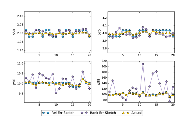
Figure 4: Actual quantiles vs. $0.005$-rank-accurate and $0.01$-relative-accurate quantiles of a data stream (20 batches of 100,000 values).

1.1 Our Results

In Section 2 we describe our relative-error sketch, dubbed the Distributed Distribution Sketch (DDSketch), and we discuss different implementation strategies. In Section 3 we prove that the sketch can handle data that is as heavy-tailed as that which comes from a distribution whose logarithm is subexponential with parameters $(\sigma,b)$, which includes heavy-tailed distributions such as the log-normal and Pareto distributions. We show that for the Pareto distribution, the size of an $\alpha$-accurate $(o(1),1)$-sketch is:

$$O\left(\frac{b\log n/\delta}{\log((1+\alpha)/(1-\alpha))}\right)$$

with probability $1-\delta$. (Note that our results hold for data coming from any distribution without any independence assumptions as long as the tail of the empirical data is no larger than that for a Pareto distribution). In Section 4 we present our experimental results.

1.2 Related Work

Quantile sketching dates back to 1980 when Munro and Paterson [29] demonstrated the first quantile sketching algorithm with formal guarantees. The best known rank-error quantile sketch is that of Greenwald and Khanna [20] whose deterministic sketch (GK) provides $\epsilon$ rank accuracy using $O((1/\epsilon)\log(n\epsilon))$ space.

In addition to accuracy and size, a desirable property of a sketch is mergeability [2]. That is, several sketches of different data sets can be combined into a single sketch that can accurately answer quantile queries over the entire data set. Mergeability has increasingly become a necessary property as systems become more distributed. Equi-depth histograms [6] are a good example of non-mergeable data set synopses as there is no way to accurately combine overlapping buckets. GK is only known to be “one-way” mergeable, that is the merging operation itself can not be distributed.

There is a line of work using randomness culminating in a rank-error quantile sketch that uses only $O((1/\epsilon)\log\log(1/\delta))$ space (where $\delta$ is the probability of failure) [25] with full mergeability. However, all of the above solutions, deterministic or randomized, have high relative error for the larger quantiles on heavy-tailed data (in practice we have found it to be worse for the randomized algorithms).

The problems of having high relative errors on the larger quantiles has been addressed by a line of work that still uses rank error, but promises lower rank error on the quantiles further away from the median by biasing the data it keeps towards the higher (and lower) quantiles [7], [8], [17]. The latter, dubbed $t$-digest, is notable as it is one of the quantile sketch implementations used by Elasticsearch [18]. These sketches have much better accuracy (in rank) than uniform-rank-error sketches on percentiles like the p99.9, but they still have high relative error on heavy-tailed data sets. Like GK they are only one-way mergeable.

The only relative-error sketch in the literature to our knowledge is the HDR Histogram [31] (and is the other quantile sketch implementation used by Elasticsearch). It has extremely fast insertion times (only requiring low-level binary operations), as the bucket sizes are optimized for insertion speed instead of size, and it is fully mergeable (though very slow). The main downside for HDR Histogram is that it can only handle a bounded (though very large) range that might not be suitable for certain data sets. It also has no published guarantees, though much of the analysis we present for DDSketch can be made to apply to a version of HDR Histogram that more closely resembles DDSketch with slightly worse guarantees.

A recent quantile sketch, called the Moments sketch [19] takes an entirely different approach by estimating the moments of the underlying distribution. It has notably fast merging times and is fully mergeable. The guaranteed accuracy, however, is only for the average rank error $\tilde{\epsilon}$, unlike all the sketches above which have guarantees for the worst-case error (whether rank or relative). The associated size bound is $O(1/\tilde{\epsilon})$. In practice, the sketch also has a bounded range as the moments quickly grow larger, and they will eventually cause floating point overflow errors.

We compare the performance of DDSketch to GK, HDR, and Moments in Section 4.

Table 1: Quantile Sketching Algorithms

	guarantee	range	mergeability
DDSketch	relative	arbitrary	full
HDR Histogram	relative	bounded	full
GKArray	rank	arbitrary	one-way
Moments	avg rank	bounded	full

A related line of work exists in constructing histograms (see [6] for a thorough survey). The accuracy of a histogram is measured using the distance between the actual values and the values of the buckets to which the original values are assigned. The task is to find the histogram with $B$ buckets that minimizes the overall distance. Optimal algorithms [24] use dynamic programming and are usually considered to be too costly, and thus approximation algorithms are often considered. The most popular distance in the literature is the squared L2 distance (such a histogram is called the v-optimal histogram), but relative-error approximation algorithms exist as well [23], [22] (though these algorithms use $\Omega(n)$ space).

Note that while one can try to use these histograms to answer quantile queries, there are no guarantees on the error of any particular quantile query, as the only error guarantees are global and not for any individual item. Moreover, the error guarantees are always relative to an unknown optimal (for the number of buckets) solution, not an absolute error guarantee. There is also no straightforward way to merge histograms as the bucket boundaries are based on the data, which can be wildly different for each histogram.

2 DDSketch

We will first describe the most basic version of our algorithm that will be able to give $\alpha$-accurate $q$-quantiles for any $0\leq q\leq 1$. It is straightforward to insert items into this sketch as well as delete items and merge sketches. Then we will show how to modify the sketch so that it gives $\alpha$-accurate $q$-quantiles for $q_{0}\leq q\leq 1$ with bounded size. Section 2.2 will go over various implementation options for the sketch.

2.1 Sketch Details

Let $\gamma:=(1+\alpha)/(1-\alpha)$. The sketch works by dividing $\mathbb{R}_{>0}$ into fixed buckets. We index our buckets by $i\in\mathbb{Z}$, and each bucket $B_{i}$ counts the number of values $x$ that fall between: $\gamma^{i-1}<x\leq\gamma^{i}$. That is, given a value $x$ we will assign it to the bucket indexed by ${\lceil{\log_{\gamma}(x)}\rceil}$:

Input: $x\in\mathbb{R}_{>0}$

$i\leftarrow{\lceil{\log_{\gamma}(x)}\rceil}$;

$B_{i}\leftarrow B_{i}+1$;

Algorithm 1 Insert($x$)

Deletion works similarly. Since the bucket boundaries are independent of the data, any two sketches using the same value for $\gamma$ can be merged by simply summing up the buckets that share an index.

A simple lemma shows that every value gets assigned to a bucket whose boundary values are enough to return a relative-error approximation to its value.

Lemma 2

For a given $q$-quantile item $x_{q}\in S$ and bucket index $i={\lceil{\log_{\gamma}(x_{q})}\rceil}$, let $\tilde{x}_{q}=2\gamma^{i}/(\gamma+1)$. Then $\tilde{x}_{q}$ is an $\alpha$-accurate $q$-quantile.

Proof 2.3.

Note that by definition of $\gamma$:

$$\alpha=1-\frac{2}{\gamma+1}=\frac{2\gamma}{\gamma+1}-1$$

Moreover, $\gamma^{i-1}<x_{q}\leq\gamma^{i}$. So if $x_{q}\geq\tilde{x}_{q}$, then:

$$\frac{x_{q}-\tilde{x}_{q}}{x_{q}}=1-\frac{\tilde{x}_{q}}{x_{q}}\leq 1-\frac{\tilde{x}_{q}}{\gamma^{i}}=1-\frac{2\gamma^{i}}{\gamma^{i}(\gamma+1)}=\alpha$$

Similarly if $x_{q}\leq\tilde{x}_{q}$, then:

$$\frac{\tilde{x}_{q}-x_{q}}{x_{q}}=\frac{\tilde{x}_{q}}{x_{q}}-1<\frac{\tilde{x}_{q}}{\gamma^{i-1}}-1=\frac{2\gamma^{i}}{\gamma^{i-1}(\gamma+1)}-1=\alpha$$

Combining both cases:

$$\left|x_{q}-\tilde{x}_{q}\right|\leq\alpha x_{q}.$$

To answer quantile queries, the sketch sums up the buckets until it finds the bucket containing the $q$-quantile value $x_{q}$:

Input: $0\leq q\leq 1$

$i_{0}\leftarrow\min(\left\{j:B_{j}>0\right\})$; $count\leftarrow B_{i_{0}}$;

$i\leftarrow i_{0}$;

while $count\leq q(n-1)$ do

       $i\leftarrow\min(\left\{j:B_{j}>0\land j>i\right\})$;

       $count\leftarrow count+B_{i}$;

end while

return $2\gamma^{i}/(\gamma+1)$;

Algorithm 2 Quantile($q$)

Given Lemma 2, the following Proposition easily follows:

Proposition 2.4.

Given $\alpha>0$ and $0\leq q\leq 1$, Quantile($q$) return an $\alpha$-accurate $q$-quantile.

Proof 2.5.

Let’s refer to the ordered elements of the multiset $S$ as $x_{(1)}\leq\dots\leq x_{(n)}$, so that by definition of the quantile, $x_{q}=x_{({\lfloor{1+q(n-1)}\rfloor})}$. We will also write $c(x)$ the number of elements in $S$ that are less than or equal to $x$. Note that for any $j$, we always have $c(x_{(j)})\geq j$. Quantile($q$) outputs $2\gamma^{i}/(\gamma+1)$ where $i=\min(\left\{j:c(\gamma^{j})>q(n-1)\right\})$. Given Lemma 2, it is enough to prove that $i={\lceil{\log_{\gamma}{x_{({\lfloor{1+q(n-1)}\rfloor})}}}\rceil}$.

Let $k$ be the largest integer so that $x_{(k)}\leq\gamma^{i}$. It is clear that $x_{(k)}$ is in the bucket of index $i$, so that $i={\lceil{\log_{\gamma}{x_{(k)}}}\rceil}$. By definition of $k$, $k=c(x_{(k)})$ and, because there is no element of $S$ in the bucket of index $i$ that is greater than $x_{(k)}$, we also know that $c(x_{(k)})=c(\gamma^{i})$. Thus, $k=c(x_{(k)})=c(\gamma^{i})>q(n-1)$ and, given that $k$ is an integer, $k\geq{\lfloor{1+q(n-1)}\rfloor}$ follows. Therefore, $i={\lceil{\log_{\gamma}x_{(k)}}\rceil}\geq{\lceil{\log_{\gamma}x_{({\lfloor{1+q(n-1)}\rfloor})}}\rceil}$.

By contradiction, if $i>{\lceil{\log_{\gamma}x_{({\lfloor{1+q(n-1)}\rfloor})}}\rceil}$, then $i-1\geq{\lceil{\log_{\gamma}x_{({\lfloor{1+q(n-1)}\rfloor})}}\rceil}$ and $\gamma^{i-1}\geq x_{({\lfloor{1+q(n-1)}\rfloor})}$. As a consequence:

$$c(\gamma^{i-1})\geq c(x_{({\lfloor{1+q(n-1)}\rfloor})})\geq{\lfloor{1+q(n-1)}\rfloor}>q(n-1),$$

which violates the definition of $i$. Hence,

$$i={\lceil{\log_{\gamma}{x_{({\lfloor{1+q(n-1)}\rfloor})}}}\rceil},$$

and the result follows.

However buckets are stored in memory (e.g., as a dictionary that maps indices to bucket counters, or as a list of bucket counters for contiguous indices), the memory size of the sketch is at least linear in the number of non-empty buckets. Therefore, a down-side to the basic version of DDSketch is that for worst-case input, its size can grow as large as $n$, the number of elements inserted into it. A simple modification will allow us to guarantee logarithmic size bounds for non-degenerate input, and Section 3 will show that the modification will never affect the ability to answer $q$-quantile queries for any constant $q$.

The full version of DDSketch is a simple modification that addresses its unbounded growth by imposing a limit of $m=f(n)$ on the number of buckets it keeps track of. It does so by collapsing the buckets for the smallest indices:

Input: $x\in\mathbb{R}_{>0}$

$i\leftarrow{\lceil{\log_{\gamma}(x)}\rceil}$;

$B_{i}\leftarrow B_{i}+1$;

if $\left|\left\{j:B_{j}>0\right\}\right|>m$ then

       $i_{0}\leftarrow\min(\left\{j:B_{j}>0\right\})$;

       $i_{1}\leftarrow\min(\left\{j:B_{j}>0\land j>i_{0}\right\})$;

       $B_{i_{1}}\leftarrow B_{i_{1}}+B_{i_{0}}$;

       $B_{i_{0}}\leftarrow 0$;

      

end if

Algorithm 3 DDSketch-Insert($x$)

Given that our sketch has predefined bucket boundaries for a given $\gamma$, merging two sketches is straightforward. We just increase the counts of the buckets for one sketch by those of the other. This, however, might increase the size of the sketch beyond the limit of $m=f(n)$, where $n$ is now the number of elements in the resulting merged sketch. As with the insertion, we stay within the limit by collapsing the buckets with smallest indices:

Input: DDSketch $S^{\prime}$

foreach $i:B_{i}>0\lor B^{\prime}_{i}>0$ do

       $B_{i}\leftarrow B_{i}+B^{\prime}_{i}$;

      

end foreach

while $\left|\left\{j:B_{j}>0\right\}\right|>m$ do

       $i_{0}\leftarrow\min(\left\{j:B_{j}>0\right\})$;

       $i_{1}\leftarrow\min(\left\{j:B_{j}>0\land j>i_{0}\right\})$;

       $B_{i_{1}}\leftarrow B_{i_{1}}+B_{i_{0}}$;

       $B_{i_{0}}\leftarrow 0$;

      

end while

Algorithm 4 DDSketch-Merge($S^{\prime}$)

We trade off the benefit of a bounded size with not being able to correctly answer $q$-quantile queries if $x_{q}$ belongs to a collapsed bucket. The next lemma shows a sufficient condition for a quantile $q$ to be $\alpha$-accurately answered by our algorithm:

Proposition 2.6.

DDSketch can $\alpha$-accurately answer a given $q$-quantile query if:

$$x_{1}\leq x_{q}\gamma^{m-1}.$$

Proof 2.7.

For any particular quantile $q$, $x_{q}$ will be $\alpha$-accurate as long as it belongs to one of the $m$ buckets kept by the sketch. Let’s refer to that bucket index as $i_{q}$, which holds values between $\gamma^{i_{q}-1}$ and $\gamma^{i_{q}}$. If the maximum bucket (that holds $x_{1}$) has index $i_{1}\leq i_{q}+m-1$, then the bucket $i_{q}$ has definitely not been collapsed. Thus, given that $x_{1}\leq x_{q}\gamma^{m-1}$, then $\gamma^{i_{1}-1}<x_{1}\leq x_{q}\gamma^{m-1}\leq\gamma^{i_{q}}\gamma^{m-1}$, and $i_{1}-1<i_{q}+m-1$, which is equivalent to $i_{1}\leq i_{q}+m-1$ as these indices are integers.

We’ll discuss the trade-offs between the accuracy $\alpha$, the minimum accurate quantile $q$, the number of items $n$, and the size of the sketch $m$ in Section 3.

2.2 Implementation Details

Most systems often have built-in timeouts and a minimum granularity, so the values coming into a sketch usually have an effective minimum and maximum. Importantly, our sketch does not need to know what those values are beforehand.

It is straightforward to extend DDSketch to handle all of $\mathbb{R}$ by keeping a second sketch for negative numbers. The indices for the negative sketch need to be calculated on the absolute values, and collapses start from the highest indices.

Like most sketch implementations, it is useful to keep separate track of the minimum and maximum values. Given how buckets are defined for DDSketch, we also keep a special bucket for zero (and all values within floating-point error of zero when calculating the index, which involves computing the logarithm of the input value).

The size of the sketch can be set to grow by setting $m=c\log n$, which will match the upper bounds discussed in Section 3, but in practice $m$ is usually set to be a constant large enough to handle a wide range of values. As an example, for $\alpha=0.01$, a sketch of size 2048 can handle values from 80 microseconds to 1 year, and cover all quantiles.

If $m$ is set to a constant, it often makes sense to preallocate the sketch buckets in memory and keep all the buckets between the minimum and maximum buckets (perhaps implemented as a ring buffer). If the sketch is allowed to grow with $n$, then the sketch can either grow with every order of magnitude of $n$, or one can implement the sketch in a sparse manner so that only buckets with values greater than 0 are kept (sacrificing speed for space efficiency).

3 Distribution Bounds

For most practical applications, e.g., tracking the latency of web requests to a particular endpoint, one cares about constant quantiles such as those around the median such as 0.25, 0.5, 0.75, or those towards the edge such as 0.9, 0.95, 0.99, 0.999. Thus by Proposition 2.6, we will focus on the necessary conditions for $x_{1}\leq x_{q}\gamma^{m-1}$ or:

$$\frac{\log(x_{1})-\log(x_{q})}{\log(\gamma)}+1\leq m.$$ (1)

for $q=\Theta(1)$, though our results will apply for $q=\Omega(1/\sqrt{n})$. (For simplicity, we will assume that $qn$ is a whole number in this section.)

For any fixed $\gamma$ and $m$, it is easy to come up with a data set $S$ for which the condition does not hold, e.g., $S=\left\{\gamma^{1},\gamma^{2},\ldots,\gamma^{2m}\right\}$. Given that distribution-free results are impossible, for our formal results, we will instead assume that our data is i.i.d. from a particular family of distributions, and then show how large the sketch would have to be for Equation 1 to hold. We are able to obtain good bounds for families of distributions as general as those whose logarithms are subexponential (e.g., Pareto distributions). While our bounds are obtained by assuming i.i.d., in practice, as long as the tail of the empirical distribution is no fatter than that of a Pareto, we do not need to assume anything about the data generating process at all.

We will bound the LHS of Equation 1 by showing that with probability greater than $1-\delta_{1}$ the sample quantile $x_{q}$ is greater than a quantile just below it. Then we will show that with probability greater than $1-\delta_{2}$, the sample maximum is less than some bound. Finally by the union bound we get that the probability that both bounds apply is greater than $1-\delta_{1}-\delta_{2}$. In practice, the probability of failing these bounds is smaller as the sample maximum and sample quantiles become quickly independent as $n$ grows.

3.1 Sample Quantiles

Let capital $X_{1},\ldots,X_{n}$ denote $n$ independent real-valued random variables drawn from a distribution with cdf $F:\mathbb{R}\rightarrow[0,1]$. The generalized inverse of $F$, $F^{-1}(p)$ is known as the quantile function of $F$. Let $X_{(1)}\leq X_{(2)}\leq\cdots\leq X_{(n)}$ denote the order statistics of $X_{1},\ldots,X_{n}$ (i.e., the ordered random variables).

The next Lemma shows that with high probability a lower sample quantile can’t fall too far below the actual quantile.

Lemma 3.8.

Let $X_{(1)}\leq X_{(2)}\leq\cdots\leq X_{(n)}$ be the order statistics for i.i.d. random variables $X_{i}$ distributed according to $F$. Let $t=\sqrt{\log(1/\delta_{1})/2n}$ and $t<q\leq 1/2$, then

$$\Pr\left[X_{(qn)}>F^{-1}(q-t)\right]\geq 1-\delta_{1}.$$

Proof 3.9.

The proof follows Chvátal’s proof of a special case of the Hoeffding bound [5]. For any single random variable $X$ drawn from a distribution with cdf $F$, $\Pr[X\leq F^{-1}(p)]=p$. Then for any particular order statistic and any $x\geq 1$:

$$\Pr\left[X_{(k)}\leq F^{-1}(p)\right]$$

$$=\sum_{i=k}^{n}\binom{n}{i}p^{i}(1-p)^{n-i}$$

$$\leq\sum_{k}^{n}\binom{n}{i}p^{i}(1-p)^{n-i}x^{i-k}+\sum_{0}^{k-1}\binom{n}{i}p^{i}(1-p)^{n-i}x^{i-k}$$

$$=x^{-k}\sum_{0}^{n}\binom{n}{i}p^{i}(1-p)^{n-i}x^{i}=x^{-k}(px+(1-p))^{n}$$ (2)

where the last equality is by the Binomial Theorem.

Equation 2 is minimized when $x=(1-p)k/p(n-k)$, and taking $k=qn$, our bound becomes:

$$\left(\frac{p(n-k)}{(1-p)k}\right)^{k}\left(\frac{(1-p)n}{n-k}\right)^{n}=\left(\frac{p}{q}\right)^{qn}\left(\frac{(1-p)}{(1-q)}\right)^{n(1-q)}$$ (3)

Note that for $x\geq 1$, $p\leq q\leq 1/2$, and that the bound is trivial when $p=q$. However, if we take $p=q-t$, we get:

$$(\ref{eqn:minimized}) =\exp\left(-qn\log\left(\frac{q}{q-t}\right)-\left(1-q\right)n\log\left(\frac{1-q}{1-q+t}\right)\right)$$

$$=\exp\left(-n\int_{q-t}^{q}\left(\frac{q}{x}-\frac{1-q}{1-x}\right)dx\right)$$

$$=\exp\left(-n\int_{q-t}^{q}\frac{q-x}{x(1-x)}dx\right)$$

$$\leq\exp\left(-4n\int_{q-t}^{q}(q-x)dx\right)=\exp\left(-2nt^{2}\right)=\delta_{1}$$

for $t=\sqrt{\log(1/\delta_{1})/2n}$, and where the last inequality uses the fact that $x(1-x)\leq 1/4$ for all $x\in\mathbb{R}$.

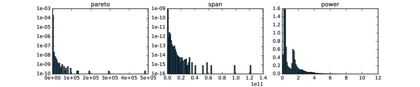
Figure 5: Histograms of the pareto, span and mpcat-obs data sets. The $y$-axes of the pareto and span data sets are plotted on log scales due to their heavy-tailed nature.

3.2 Sample Maximums

We will first bound the sample maximum for subexponential distributions, which include the Gaussian, logistic, chi-squared, exponential, and many others.

Definition 3.10.

A random variable $X\in\mathbb{R}$ is said to be subexponential with parameters $(\sigma,b)$ if

$$\mathbb{E}\left[\exp\left(\lambda(X-\mathbb{E}X)\right)\right]\leq\exp\left(\sigma^{2}\lambda^{2}/2\right),$$

for $0\leq\lambda\leq 1/b$.

Using Chernoff-type techniques, one can obtain concentration inequalities for subexponential variables [4].

Theorem 3.11.

Let $X$ be a subexponential random variable with parameters $(\sigma,b)$. Then,

$$\Pr\left[X-\mathbb{E}X\geq t\right]\leq\exp\left(-t^{2}/2\sigma^{2}\right)$$

for $0\leq t\leq\sigma^{2}/b$, and

$$\Pr\left[X-\mathbb{E}X\geq t\right]\leq\exp\left(-t/2b\right)$$

for $t>\sigma^{2}/b$.

Now we can lower-bound the sample maximum by the complement of the event that none of the sample is greater than $t$.

Corollary 3.12.

Let $X_{(1)}\leq X_{(2)}\leq\cdots\leq X_{(n)}$ be the order statistics for i.i.d. subexponential random variables $X_{i}$ with parameters $(\sigma,b)$, and $t=2b\log(n/\delta_{2})$. Then the sample maximum is less than $t$ with probability at least $1-\delta_{2}$.

Proof 3.13.

By Theorem 3.11,

$$\Pr\left[X_{(n)}-\mathbb{E}X>t\right] <1-\left(1-e^{-t/2b}\right)^{n}$$

$$=1-\left(1-\frac{\delta_{2}}{n}\right)^{n}<\delta_{2},$$

where the final inequality is by Bernoulli’s inequality.

3.3 Sketch Size Bounds

For subexponential distributions, we can bound Equation 1 by combining Lemma 3.8 and Corollary 3.12:

Theorem 3.14.

Let $X_{(1)}\leq X_{(2)}\leq\cdots\leq X_{(n)}$ be the order statistics for i.i.d. random variables $X_{i}$ distributed according to a subexponential distribution $F$ with parameters $(\sigma,b)$. Then with probability at least $1-\delta_{1}-\delta_{2}$, DDSketch is an $\alpha$-accurate $(q,1)$-sketch with size at most $(\log X_{(n)}-\log X_{(qn)})/\log(\gamma)+1$, which is bounded from above by:

$$\frac{\log\left(2b\log\left(n/\delta_{2}\right)+\mathbb{E}X\right)-\log\left(F^{-1}\left(q-t\right)\right)}{\log(\gamma)}+1$$

for $\gamma=(1+\alpha)/(1-\alpha)$, $t=\sqrt{\log(1/\delta_{1})/2n}$, and $t<q\leq 1/2$.

Exponential. For concreteness, let’s take $\delta_{1}=\delta_{2}=e^{-10}$ and $\alpha=0.01$ (i.e., $\gamma\approx 1.02$), and let’s consider the exponential distribution with cdf $F(t;\lambda)=1-\exp(-\lambda t)$ for $t\geq 0$, and 0 otherwise. The exponential distribution is subexponential with parameters $(2/\lambda,2/\lambda)$.

If $n>320$, then $p>3/8$, and the sample median is at least $F^{-1}\left(p\right)>-\lambda^{-1}\log(1-3/8)>0.47/\lambda$. The sample maximum is at most $4\lambda^{-1}(\log(n)+10+1/4)$, and $1/\log(\gamma)<51$ so we can bound the size from Theorem 3.14 by: $51(\log(4\log n+41)-\log(0.47))+1$.

This means that even with a sketch of size 273 one can 0.01-accurately maintain the upper half order statistics of over a million samples with probability greater than 0.99991. This grows double-exponentially, so a sketch of size 1000 can 0.01-accurately maintain the upper half order statistics of over $\exp(\exp(17))$ values with that same probability.

Pareto. The double logarithm in our size bound from Theorem 3.14 allows us to handle distributions with much fatter tails as well. The Pareto distribution distribution has cdf $F(t;a,b)=1-(b/t)^{a}$. If $X$ is a random variable drawn from this distribution, then $Y=\log(X/b)\sim Exp(a)$. Thus, we can reuse the arguments above to get that with probability at least $1-\delta_{1}-\delta_{2}$:

$$\log(X_{(n)})<4a^{-1}\log(n/\delta_{2})+a^{-1}+\log(b)$$

and

$$\log(X_{(n/2)})>-a^{-1}\log(1/2+\sqrt{\log(1/\delta_{1})/2n})+\log(b).$$

As before, let’s take $\delta_{1}=\delta_{2}=e^{-10}$, $\alpha=0.01$, and assume that $n>320$. With probability greater than $1-e^{-10}-e^{-10}\approx 0.99991$:

$$\frac{\log(X_{(n)})-\log(X_{(n/2)})}{\log(\gamma)}+1<51a^{-1}(4\log n+11)+1$$

Given that Pareto distributions have exponentially fatter tails than exponential distributions, the sketch size upper bounds increase accordingly. Taking $a=1$, this means that we require a sketch of size 3380 to 0.01-accurately maintain the upper half order statistics of over a million samples with probability greater than 0.99991. A sketch of size 10000, can 0.01-accurately maintain the upper half order statistics of over $\exp(46)$ values with that same probability.

Other Distributions. We focused on subexponential tails and the Pareto distribution in this section as we believe it to best represent the worst case for practical use-cases of quantile sketching. For lighter tails such as subgaussians and thus for lognormal distributions, we can of course get much tighter bounds.

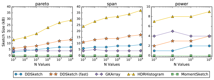
Figure 6: Sketch size in memory in kB.

4 Evaluation

We provide implementations of DDSketch in Java [12], Go [13] and Python [14]. Our Java implementation provides multiple versions of DDSketch: buckets can be stored in a contiguous way (for fast addition) or in a sparse way (for smaller memory footprint). The number of buckets can grow indefinitely or be bounded with a fixed maximum of $m$ buckets, collapsing the buckets of lowest or highest indices. The mapping of the values to their bucket indices can be logarithmic, as defined above, but we also provide alternative mappings that are faster to evaluate while still ensuring relative accuracy guarantees. Those mappings make the most of the binary representation of floating-point values, which provides a costless way to evaluate the logarithm to the base 2. In between a linear or quadratic interpolation can be used so that the logarithm to any base can be approximated. Those mappings define buckets whose sizes are not optimal under the constraint of ensuring relative accuracy guarantee as some of them are smaller than necessary. Their faster evaluation than the memory-optimal logarithmic mapping comes at the cost of requiring more buckets to cover a given range of values, and therefore a memory footprint overhead in DDSketch. We refer to this version of the code as DDSketch (fast) in our experiments.

We compare DDSketch against the Java implementation [31] of HDR Histogram, our Java implementation of the GKArray version of the GK sketch [12], as well as the Java implementation of the Moments sketch [15] (all three discussed in Section 1.2). HDR Histogram is a relative-error sketch for non-negative values. Its accuracy is expressed as the number of significant decimal digits $d$ of the values. GKArray guarantees that the rank error of the estimated quantiles will be smaller than $\epsilon$ after adding values. The Moments sketch has guarantees on the average rank error bounded by the number of moments $k$ that are estimated.

We consider three data sets, and compare the size in memory of the sketches, the speed of adding values and merging sketches, and the accuracy of the estimated quantiles. The measurements are performed with the Java implementations of all four sketches.

The sketch parameters are chosen so that the targeted relative accuracy for DDSketch and HDR Histogram is 1%. For GKArray, we use a rank accuracy that gives roughly similar memory footprints as DDSketch. For the Moments sketch, we use the maximum recommended numbers of moments, as per the Java implementation documentation, and we also use the arcsinh transform (called compression in the code), which makes the sketch more accurate for distributions with heavy tails. Those parameters are summarized in Table 2.

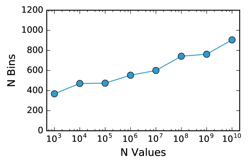
Figure 7: Number of bins in DDSketch for the pareto data set.

Table 2: Experiment Parameters

DDSketch	$\alpha=0.01$
	$m=2048$
HDR Histogram	$d=2$
GKArray	$\epsilon$ = 0.01
Moments sketch	$k$ = 20
	compression enabled

4.1 Data Sets

We use three data sets for our experiments, whose distributions are shown in Figure 5. The pareto data set contains synthetic data generated from a Pareto distribution with $a=b=1$. The span data set is a set of span durations of the distributed traces of requests that Datadog received over a few hours. The durations are integers in units of nanoseconds, and it includes a wide range of values (from $100$ to $1.9\times 10^{12}$). The power dataset is the global active power measurements from the UCI Individual Household Electric Power Consumption dataset [26].

4.2 Sketch Size In Memory

How much space a sketch takes up in memory will be an important consideration in many applications. For each of the four sketches, the parameters chosen will determine the accuracy of the sketch as well as its size. An increase in accuracy generally requires a larger sketch. Figure 6 plots the sketch size in memory as $n$ increases.

We see that DDSketch (fast) can be up to twice the size of DDSketch, and that HDR Histogram is significantly larger. Both GKArray and the Moments sketch are much smaller, and the Moments sketch in particular is completely independent of the size of the input.

If one runs DDSketch with a limit placed on the number of bins the sketch can contain, when the maximum number of bins is reached, DDSketch starts to combine the smallest bins together as needed, meaning that the lower quantile estimates may not meet the relative accuracy guarantee. In our experiments this maximum was never reached, and we have not found this to be an issue. Figure 7 plots the number of DDSketch bins for the pareto data set. The number of bins is around 900 for $n=10^{10}$, less than half the limit of 2048. It is also worth noting that the actual sketch size required for the Pareto distribution is much smaller than the upper bounds we calculated in Section 3.3.

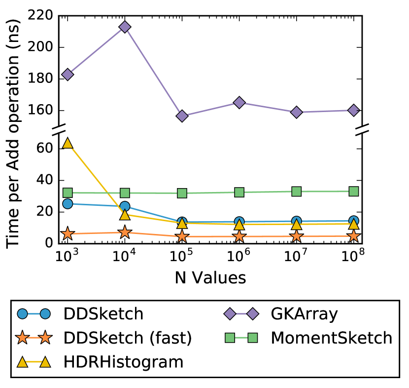
Figure 8: Average time required to add a value to a sketch.

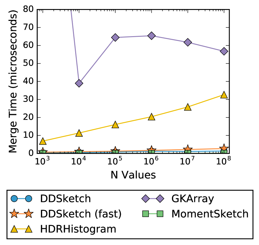
Figure 9: Average time required to merge two sketches as a function of number of values in the merged sketch.

4.3 Add and Merge Speeds

In this section, we compare the performance of the sketches in terms of the time required to add values to a sketch and to merge sketches together. Figure 8 shows the average time required to add $n$ values to an empty sketch divided by $n$. It takes less than 5 seconds to add a hundred million values to an empty DDSketch on a 3.1GHz MacBook Pro.

GKArray is the slowest for insertions by far, being around six times slower than the Moments sketch. Adding to an HDR Histogram is faster than adding to the standard version of DDSketch as HDR Histogram has a simpler index calculation than DDSketch which has to calculate logarithms. DDSketch (fast) is the fastest in terms of insertion speed, though this was obtained by an increase in the sketch size as we saw in Section 6.

Figure 9 plots the average time required to merge two sketches of roughly the same size, as a function of the number of values in the merged sketch. Merging two DDSketches is very fast—it takes around 10 microseconds or less to merge two sketches containing up to fifty million values each—depending on the data set and size, it can be more than an order of magnitude faster than GKArray or HDR Histogram. The Moment sketch has the fastest merge speeds of all the algorithms, as each sketch only holds on to $k=20$ values.

4.4 Sketch Accuracy

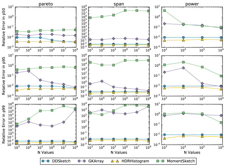
Figure 10: Relative errors of p50, p95, and p99 estimates.

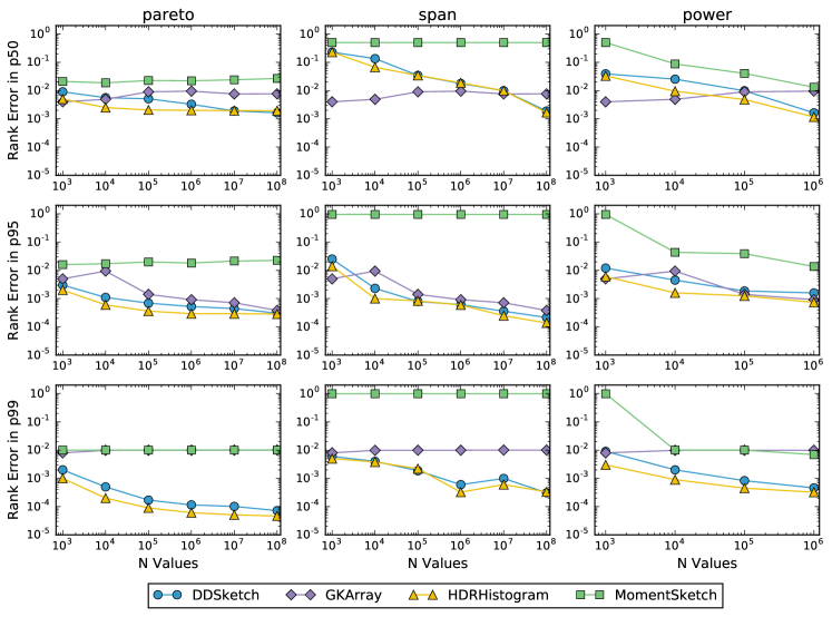
Figure 11: Rank errors of p50, p95, and p99 estimates.

DDSketch guarantees a relative error in its quantile estimates of at most $\alpha$, while GKArray guarantees a rank error of less than $\epsilon$. HDR Histogram has an implied relative-error guarantee of $10^{-d}$ where $d$ is the number of significant digits. Therefore we compare both the average relative and rank errors in Figures 10 and 11, for the p50, p95, and p99 estimates. Note that for GKArray, for $n\leq 1/\epsilon$, all the values are retained so that both the relative error and rank error will be zero.

Figure 10 shows that for all three data sets DDSketch has a consistent relative error less than $\alpha$ for all values of $n$. For the heavy-tailed pareto and span data sets, the relative error sketches (DDSketch and HDR Histogram) have much smaller relative error than either GKArray or Moments. The discrepancy is especially striking for the higher quantiles, as the values returned can be several orders of magnitude off the actual value. The Moments sketch has particular difficulty with the span data set as it has trouble dealing with such a large range of values.

In terms of rank error, the guarantee of GKArray can be clearly seen in Figure 11. No such guarantee is provided for DDSketch and HDR Histogram, yet they perform better than the Moments sketch which has a guarantee on average, and even GK for the higher quantiles.

5 Conclusion

Datadog’s use-case for distributed quantile sketching comes from our agent-based monitoring where we need to accurately aggregate data coming from disparate sources in our high-throughput, low-latency, distributed data processing engine. To get a sense of the scale, some of our customers have endpoints that handle over 10M points per second, and DDSketch provides accurate latency quantiles for these endpoints.

After our initial evaluation of existing quantile sketching algorithms, we settled on the Greenwald-Khanna algorithm as it could handle arbitrary values, and provided the best compromise between accuracy, size, insertion speed, and merge time. (The implementation we provide comes from our work in optimizing the algorithm.)

Unfortunately, the relative-accuracy errors for higher quantiles generated by the rank-error sketch proved to be unacceptable, which led us to develop DDSketch. Unlike HDR Histogram, which is designed to handle a bounded range and has poor merge speeds, DDSketch is a flexible relativer error sketch that can handle arbitrarily large ranges, and has fast merge speeds. Compared to GK, the relative accuracy of DDSketch is comparable for dense data sets, while for heavy-tailed data sets the improvement in accuracy can be measured in orders of magnitude. The rank error is also comparable to if not better than that of GK. Additionally, it is much faster in both insertion and merge.

6 Acknowledgment

This research has made use of data provided by the International Astronomical Union’s Minor Planet Center.

References

- [1] L. Abraham, J. Allen, O. Barykin, V. Borkar, B. Chopra, C. Gerea, D. Merl, J. Metzler, D. Reiss, S. Subramanian, J. L. Wiener, and O. Zed. Scuba: Diving into data at facebook. PVLDB, 6(11):1057–1067, 2013.
- [2] P. K. Agarwal, G. Cormode, Z. Huang, J. Phillips, Z. Wei, and K. Yi. Mergeable summaries. In Proceedings of the 31st ACM SIGMOD-SIGACT-SIGAI Symposium on Principles of Database Systems, PODS ’12, pages 23–34, New York, NY, USA, 2012. ACM.
- [3] B. Beyer, C. Jones, J. Petoff, and N. R. Murphy. Site Reliability Engineering: How Google Runs Production Systems. ” O’Reilly Media, Inc.”, 2016.
- [4] V. V. Buldygin and U. V. Kozachenko. Metric Characterization of Random Variables and Random Processes. American Mathematical Society, Rhode Island, USA, 2000.
- [5] V. Chvátal. The tail of the hypergeometric distribution. Discrete Mathematics, 25:285–287, 1979.
- [6] G. Cormode, M. Garofalakis, P. J. Haas, and C. Jermaine. Synopses for massive data: Samples, histograms, wavelets, sketches. Foundations and Trends® in Databases, 4(1-3):1–294, 2011.
- [7] G. Cormode, F. Korn, S. Muthukrishnan, and D. Srivastava. Effective computation of biased quantiles over data streams. In 21st International Conference on Data Engineering, ICDE’05, pages 20–31, New York, NY, USA, 2005. IEEE Computer Society Press.
- [8] G. Cormode, F. Korn, S. Muthukrishnan, and D. Srivastava. Space- and time-efficient deterministic algorithms for biased quantiles over data streams. In Proceedings of the 25th ACM SIGMOD-SIGACT-SIGART Symposium on Principles of Database Systems, PODS ’06, pages 263–272, New York, NY, USA, 2006. ACM.
- [9] C. Cranor, T. Johnson, O. Spataschek, and V. Shkapenyuk. Gigascope: a stream database for network applications. In Proceedings of the 2003 ACM SIGMOD International Conference on Management of Data, pages 647–651. ACM, 2003.
- [10] Datadog. 8 emerging trends in container orchestration. https://www.datadoghq.com/container-orchestration, 2018. Accessed: 2018-12-12.
- [11] Datadog. 8 surprising facts about real docker adoption. https://www.datadoghq.com/docker-adoption/, 2018. Accessed: 2018-12-12.
- [12] Datadog. https://github.com/DataDog/sketches-java, 2019.
- [13] Datadog. https://github.com/DataDog/sketches-go, 2019.
- [14] Datadog. https://github.com/DataDog/sketches-py, 2019.
- [15] S. DAWN. Moments sketch. https://github.com/stanford-futuredata/momentsketch, 2018. Accessed: 2019-05-29.
- [16] J. Dean and L. A. Barroso. The tail at scale. Communications of the ACM, 56(2):74–80, 2013.
- [17] T. Dunning and O. Ertl. Computing extremely accurate quantiles using t-digests. arXiv preprint arXiv:1902.04023, 2019.
- [18] Elasticsearch. Elasticsearch reference: Percentiles aggregation. https://www.elastic.co/guide/en/elasticsearch/reference/current/search-aggregations-metrics-percentile-aggregation.html, 2015. Accessed: 2018-09-14.
- [19] E. Gan, J. Ding, K. S. Tai, V. Sharan, and P. Bailis. Moment-based quantile sketches for efficient high cardinality aggregation queries. PVLDB, 11(11):1647–1660, 2018.
- [20] M. B. Greenwald and S. Khanna. Space-efficient online computation of quantile summaries. In Proceedings of the 2001 ACM SIGMOD International Conference on Management of Data, SIGMOD ’01, pages 58–66, New York, NY, USA, 2001. ACM.
- [21] M. B. Greenwald and S. Khanna. Quantiles and equidepth histograms over streams. In M. Garofalakis, J. Gehrke, and R. Rastogi, editors, Data Stream Management, pages 45–86. Springer, New York, NY, USA, 2016.
- [22] S. Guha, N. Koudas, and K. Shim. Approximation and streaming algorithms for histogram construction problems. ACM Transactions on Database Systems (TODS), 31(1):396–438, 2006.
- [23] S. Guha, K. Shim, and J. Woo. Rehist: Relative error histogram construction algorithms. In Proceedings of the 30th International Conference on Very Large Data Bases, VLDB ’04, pages 300–311. VLDB Endowment, 2004.
- [24] H. V. Jagadish, N. Koudas, S. Muthukrishnan, V. Poosala, K. C. Sevcik, and T. Suel. Optimal histograms with quality guarantees. In Proceedings of the 24rd International Conference on Very Large Data Bases, VLDB ’98, pages 275–286, 1998.
- [25] Z. Karnin, K. Lang, and E. Liberty. Optimal quantile approximation in streams. In Proceedings of the 57th IEEE Symposium on Foundations of Computer Science (FOCS), FOCS ’16, pages 71–78, New York, NY, USA, 2016. IEEE Computer Society Press.
- [26] M. Lichman. Uci machine learning repository. https://archive.ics.uci.edu/ml/datasets/individual+household+electric+power+consumption, 2013.
- [27] G. Luo, L. Wang, K. Yi, and G. Cormode. Quantiles over data streams: experimental comparisons, new analyses, and further improvements. PVLDB, 25(4):449–472, 2016.
- [28] S. Madden, M. J. Franklin, J. M. Hellerstein, and W. Hong. The design of an acquisitional query processor for sensor networks. In Proceedings of the 2003 ACM SIGMOD International Conference on Management of Data, pages 491–502. ACM, 2003.
- [29] J. I. Munro and M. S. Paterson. Selection and sorting with limited storage. Theoretical Computer Science, 12(3):315–323, 1980.
- [30] R. R. Sambasivan, R. Fonseca, I. Shafer, and G. R. Ganger. So, you want to trace your distributed system? key design insights from years of practical experience. Technical Report CMU-PDL-14-102, Carnegie Mellon University, 2014.
- [31] G. Tene. Hdrhistogram: A high dynamic range (hdr) histogram. http://hdrhistogram.org/, 2012. Accessed: 2018-09-15.