Local-field Theory of the BCS-BEC Crossover

Abstract

We develop a self-consistent theory unifying the description of a quantum Fermi gas in the presence of a Fano-Feshbach resonance in the whole phase diagram ranging from BCS to BEC type of superfluidity and from narrow to broad resonances, including the fluctuations beyond mean field. Our theory covers a part of the phase diagram which is not easily accessible by Quantum Monte Carlo simulations and is becoming interesting for a new class of experiments in cold atoms.

Ultracold gases, trapped gases Degenerate Fermi gases Quantum fluids: general properties

Quantum gases keep building up considerable interest, as combined experimental-theoretical platforms where the borders between condensed matter, fundamental physics and cosmology can be crossed, with mutual fertilization under the extremely controlled experimental settings and microscopic modeling of atomic physics Adams et al. (2012). Bright examples include a new class of precision measurements Pezzè et al. (2018), Hamiltonian coding inspired by Feynman’s idea of quantum simulators Bloch I. and S. (2012); Zohar et al. (2013); Bernien et al. (2017) for real-time dynamics Zohar et al. (2013); Martinez et al. (2016), and the quantum phases of Bose/Fermi-Hubbard models relevant to condensed matter Endres et al. (2012); Chiu et al. (2018); Messer et al. (2018).

Among the intersecting concepts, unexpectedly central remains the paradigm of the crossover from Bose-Einstein Condensation (BEC) to Bardeen-Cooper-Schrieffer (BCS) type superfluidity Strinati et al. (2018); Chen et al. (2005). Developed by Leggett Leggett (1980) and Nozières and Schmitt-Rink Nozieres1985 (1985b), its relevance to high-temperature superconductivity (HTSC) was pointed out by Uemura et al. Uemura et al. (1991) in a celebrated universal plot, explained in terms of the correlation length Pistolesi and Strinati (1994), and has become a timely concept for the quantum chromodynamics phase diagram Baym (2010) and the equation of state in neutron stars Gezerlis and Schwenk (2014); Schwenk and Pethick (2005).

The advent of Fermi gases Greiner et al. (2003); Zwierlein et al. (2003); Bourdel et al. (2004); Jochim et al. (2003) has turned the crossover physics from a phenomenological approach to gain insight on microscopic theories, into a paradigm to be explored under microscopic mechanisms. Among the latter is the Fano-Feshbach (FF) resonance concept Fano (1961); Feshbach (1962), where scattering length $a$ and contact interaction strength $U=4\pi\hbar^{2}a/m$ can be varied at will. The resonance originates from the coupling between a free scattering state of two atoms (open channel) and their bound (closed channel) state (see Fig. 1). FF resonances can be classified as narrow (broad) depending on the coupling strength being weak (strong) on the Fermi energy scale $\varepsilon_{F}\equiv\hbar^{2}k_{F}^{2}/(2m)$. Alternatively, the energy dependence of scattering processes can be embodied in the effective range $r_{0}$ of the interactions, so that narrow (broad) resonances imply $k_{F}|r_{0}|\gg 1$ ($\ll 1$).

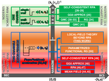
Figure 1: Conceptual map of BEC-BCS crossover theories in the relevant parameter space defined by $-(k_{F}a)^{-1}$, driving the crossover between BEC and BCS limits, and $(k_{F}r_{0})^{-1}$, driving the resonance width from narrow to broad Gurarie and Radzihovsky (2007). Sketched are the general model-frameworks (left), i.e. one or two-channel, and the theoretical or Quantum Monte Carlo (QMC) methods (right) used to explore the crossover in narrow (red stripe), intermediate (orange), and broad (green) region (see text). This work bridges the gap of intermediate-to-large values of $(k_{F}r_{0})^{-1}$, including fluctuations via a unifying local-field theory of the boson-fermion hamiltonian.

The conceptual map in Fig. 1 summarizes theories developed so far in this scenario for cold gases. One-channel models build on the BCS Hamiltonian using $U$ as unique parameter, thus suited to describe broad resonances, where the interparticle spacing is the only relevant parameter. Broad resonances have been the norm so far in experiments, very well explored via self-consistent theories including pairing fluctuations Chen et al. (1998); Haussmann (1993); Pieri et al. (2004); Perali et al. (2004a); Haussmann et al. (2007) and Quantum Monte Carlo (QMC) simulations at zero and finite temperature Astrakharchik et al. (2004); Bulgac et al. (2006); Burovski et al. (2006); Akkineni et al. (2007) and by Renormalization Group methods Nikolić and Sachdev (2007). Intermediate resonances are becoming available in quantum gases experiments Baier et al. (2018a); Mazurenko et al. (2017); Lercher, A.D. et al. (2011). Besides, superfluidity in neutron stars Gezerlis and Schwenk (2014), is characterized by $k_{F}|r_{0}|\simeq 1$. Their theoretical treatment, however, still leaves a number of open questions, stemming from the need of encapsulating the finite width as a second parameter Gurarie and Radzihovsky (2007); Diener and Ho (2004); Chin et al. (2010). Though QMC results are available Forbes et al. (2011) in a one-channel model mimicking the finite width via well-barrier potentials (Fig. 1), they are limited to $(k_{F}|r_{0}|)^{-1}\gg 1$. Two-channel, boson-fermion (BF) models instead explicitly include the resonant (boson) state composed by two fermions, embodying the original FF mechanism. Introduced in the HTSC context Friedberg and Lee (1989); Ranninger and Robin (1995), the BF model has been proposed for ultracold atoms in a mean-field formulation Timmermans et al. (1999); Holland et al. (2001), developed within a Random-Phase-Approximation (RPA) Ohashi and Griffin (2003a); Ohashi and Griffin (2002), and upgraded to different forms of self-consistent RPA Stajic et al. (2004); Liu and Hu (2005). Inclusion of particle-hole fluctuations suited to treat a wide range of FF resonance widths, has been performed within the powerful Functional Renormalization Group (FRG) approach, though in a parametrized manner Floerchinger et al. (2008); Diehl et al. (2007a, b). As a matter of facts, the intermediate regime bridging from narrow to broad FF resonance is devoided of simulational methods and largely unexplored by unifying theoretical methods that include fluctuations beyond mean field.
Here we contribute to fill up this theoretical gap. At variance with Floerchinger et al. (2008), we develop a theory hinging on a single approximation. With respect to the largely explored broad limit, we predict sizeable effects in $T_{c}$ at intermediate resonance widths, now accessible in current experiments Baier et al. (2018a); Mazurenko et al. (2017); Lercher, A.D. et al. (2011), both at unitarity and in the BCS limit. We take inspiration from local-field dielectric theories For an overview see Giuliani and Vignale (2005), in particular Singwi-Tosi-Land-Sjölander (STLS) Singwi et al. (1968); Hasegawa and Shimizu (1975) formalism, developed in the 70s to describe the low-density normal electron liquid. In our theory, the superfluid-state symmetries are naturally built in and the Gor’kov and Melik-Barkhudarov screening corrections Gor’kov and Melik-Barkhudarov (1961) recovered. We discuss applications to current experiments and its potential extensions to describe exotic phases away from the superfluid phase.
The theory- We consider the boson-fermion (BF) grand-canonical Hamiltonian Friedberg and Lee (1989):

$$\begin{split}\mathcal{H}-\mu\,\mathcal{N}&=\sum_{\mathbf{k},\sigma}\varepsilon_{\mathbf{k}}\,c^{\dagger}_{\mathbf{k},\sigma}c_{\mathbf{k},\sigma}+\sum_{\mathbf{q}}\varepsilon_{\mathbf{q}}^{B}\,b_{\mathbf{q}}^{\dagger}b_{\mathbf{q}}+\\ +&\frac{g}{\sqrt{V}}\sum_{\mathbf{k},\mathbf{q}}\left[b^{\dagger}_{\mathbf{q}}\,c_{\mathbf{q}/2-\mathbf{k},\downarrow}\,c_{\mathbf{q}/2+\mathbf{k},\uparrow}+\text{h.c.}\right]+\\ -&\frac{U_{bg}}{V}\sum_{\mathbf{k},\mathbf{k}^{\prime},\mathbf{q}}c^{\dagger}_{\mathbf{q}/2+\mathbf{k},\uparrow}\,c^{\dagger}_{\mathbf{q}/2-\mathbf{k},\downarrow}\,c_{\mathbf{q}/2-\mathbf{k}^{\prime},\downarrow}\,c_{\mathbf{q}/2+\mathbf{k}^{\prime},\uparrow}.\end{split}$$ (1)

The operator $c^{\dagger}_{\mathbf{k},\sigma}$ ($b_{\mathbf{k}}^{\dagger}$) creates a spin-1/2 fermion (spinless boson) with momentum $\mathbf{k}$. The first two terms represent the fermion and boson kinetic energies $\varepsilon_{\mathbf{k}}=k^{2}/(2m)-\mu$ and $\varepsilon_{\mathbf{q}}^{B}=q^{2}/(4m)-2\mu+2\nu$, in terms of the fermionic mass $m$, chemical potential $\mu$ and energy $2\nu$ of the resonant state. The factors $4m$ and $2\mu$ in the dispersion account for the bosons being composed of two fermions. $2\nu$ is the crucial parameter driving the system from the Fermi limit at large detunings $\nu\gg\varepsilon_{F}$, where bosons exist only as virtual states, to the pure Bose limit $\nu$$\ll$$-\varepsilon_{F}$ with a real macroscopic occupation of the resonant state. Bosons and fermions are hybridized via the coupling with strength $g$, converting two fermions into a boson and viceversa, related to the effective range $r_{0}$ of the scattering potential via $r_{0}=-8\pi\hbar^{4}/(mg)^{2}$ Gurarie and Radzihovsky (2007); Kokkelmans et al. (2002). The theory embodies two independent physical parameters, $k_{F}r_{0}$ and $k_{F}a$, in the model tuned via $g$ and $\nu$. To which the background scattering length $a_{bg}$ ($U_{bg}\equiv 4\pi\hbar^{2}a_{bg}/m$) joins to account for scattering away from resonance.
The method- Our method hinges on the concept of local field in dielectic-function theories, introduced to study the density and spin response of the electron liquid in low-density metals, where the Coulomb interaction dominates over the kinetic energy Hubbard (1957); Singwi et al. (1968). While referring to the Supplemental Material (SM) SoM for details, here is the concept essence. The system response is determined by introducing the exchange and correlation (xc) potential $V_{\text{xc}}(\vec{r},t)=-\int dt^{\prime}d\vec{r}\,v(|\vec{r}-\vec{r}^{\prime}|)G_{L}(|\vec{r}-\vec{r}^{\prime}|,t-t^{\prime})\delta n(\vec{r}^{\prime},t^{\prime})$, in terms of the so-called local-field factor $G_{L}$ generated by the polarization density locally induced in the medium and describing the hole dug in around a given particle by xc processes. In the STLS scheme Singwi et al. (1968), $G_{L}$ is determined by the xc-generalized force driven by the fluid and weighted over the static probability of finding a particle at distance $r$, measured by the pair-correlation function $g(\vec{r})$ For an overview see Giuliani and Vignale (2005); SoM . The equations set is closed by relating $g(\vec{r})$ to the structure factor, and the latter to the imaginary part of the response via the fluctuation-dissipation theorem. In different language, the choice of $G_{L}$ amounts to define the irreducible interaction determining the vertex corrections. Inspired by these physical ideas, we now turn to implement them in the BF theory.
As detailed in the SM  SoM , our method naturally embodies the spin-$SU(2)$ and time-reversal symmetries dictated by the Hamiltonian  (1), and those emerging from gauge transformations, like the Hugenoltz-Pines theorem Hugenholtz and Pines (1959) ensuring that the excitation spectrum be gapless while the Goldstone mode sets in. The resulting complex formalism can be represented in a quite compact form, but in order to comprehensively reveal the essence of the theory, we reduce it to a minimum by first focusing on the calculation of the superfluid transition temperature $T_{c}$.
Since the Thouless criterion states that the divergence of the the pairing susceptibility $\Pi\left(\mathbf{q},\omega\right)$ is related to the divergence of the particle-particle scattering vertex, we start by evaluating $\Pi\left(\mathbf{q},\omega\right)=i\int_{0}^{\infty}dt\,e^{i\omega t}\,\langle{\mathcal{C}^{\dagger}_{\mathbf{q}}\left(t\right)}{\mathcal{C}_{\mathbf{q}}\left(0\right)}\rangle$, where the operator $\mathcal{C}_{\mathbf{q}}\equiv\sum_{\mathbf{k}}\left[c_{-\mathbf{k}+\mathbf{q}/2,\downarrow}c_{\mathbf{k}+\mathbf{q}/2,\uparrow}\right]$ annihilates a fermion pair with total momentum $\mathbf{q}$ and averages are meant at equilibrium as in linear response. We perturb the pairing fields by acting with the source term $J_{\mathbf{q}}(t)$ explicitly breaking the $U(1)$ symmetry, i.e. adding $\sum_{\mathbf{q}}\left[J^{*}_{\mathbf{q}}(t)\mathcal{C}_{\mathbf{q}}(t)+J_{\mathbf{q}}(t)\mathcal{C}^{\dagger}_{\mathbf{q}}(t)\right]$ to (1). We then compute the system linear response by the equation of motion method. In fact, the generalized Wigner distribution function $f^{*}_{\mathbf{k},\mathbf{q}}(t)=\langle c^{\dagger}_{\mathbf{k}+\mathbf{q}/2,\uparrow}(t)c^{\dagger}_{-\mathbf{k}+\mathbf{q}/2,\downarrow}(t)\rangle$, turns out to be more practical to work with, than $\mathcal{C}^{(\dagger)}$. After Fourier transforming in frequency domain, we obtain:

$$\omega f^{*}_{\mathbf{k},\mathbf{q}}=\left(\varepsilon_{\mathbf{k}+\mathbf{q}/2}+\varepsilon_{\mathbf{k}-\mathbf{q}/2}\right)f^{*}_{\mathbf{k},\mathbf{q}}$$

$$+\sum_{\mathbf{q}^{\prime},\sigma}\left(\frac{1}{2}\delta_{\mathbf{q},\mathbf{q}^{\prime}}-\big{\langle}\mathcal{D}^{\sigma}_{\text{sgn}\sigma\mathbf{k}+\mathbf{q^{\prime}}/2,\mathbf{q}-\mathbf{q}^{\prime}}\big{\rangle}\right)J^{*}_{\mathbf{q}^{\prime}}(\omega)$$ (2)

$$+\sum_{\mathbf{q}^{\prime},\sigma}\bigg{\langle}\left(\frac{1}{2}\delta_{\mathbf{q},\mathbf{q}^{\prime}}-\mathcal{D}^{\sigma}_{\text{sgn}\sigma\mathbf{k}+\mathbf{q^{\prime}}/2,\mathbf{q}-\mathbf{q}^{\prime}}\right)U_{\text{eff}}(\mathbf{q}^{\prime},\omega)\mathcal{C}^{\dagger}_{\mathbf{q}^{\prime}}\bigg{\rangle},$$

where $\mathcal{D}^{\sigma}_{\mathbf{k},\mathbf{q}}\equiv c^{\dagger}_{\mathbf{k}+\mathbf{q}/2,\sigma}c_{\mathbf{k}-\mathbf{q}/2,\sigma}$, $\text{sgn}(\uparrow)=+1$, $\text{sgn}(\downarrow)=-1$, and $\delta_{\mathbf{q},\mathbf{q}^{\prime}}\equiv(2\pi)^{3}\delta^{3}(\mathbf{q}-\mathbf{q}^{\prime})$. The effective interaction $U_{\text{eff}}(\mathbf{q},\omega)=-U_{bg}+g^{2}D_{0}(\mathbf{q},\omega)=-U_{bg}+{g^{2}}/({\omega-\varepsilon^{B}_{\mathbf{q}}})$ is driven by the bare contact and the exchange of a resonant boson. In the above equation, we have omitted the $\omega$-dependence of $f_{\mathbf{k},\mathbf{q}}$ for the sake of simplicity. Average over the unperturbed system yields $\langle\mathcal{D}^{\alpha}_{\mathbf{k},\mathbf{q}}\rangle=n_{\mathbf{k}}\,\delta_{\mathbf{q},0}$, with $n_{\mathbf{k}}=2T\sum_{i\omega_{n}}G(\mathbf{k},i\omega_{n})e^{i\omega_{n}0^{+}}$ the momentum distribution, that can be computed from the fermionic Green’s function $G(\mathbf{k},i\omega_{n})$ once the self-energy is known. Postponing this task, we begin by approximating $n_{\mathbf{k}}=f(\varepsilon_{\mathbf{k}})=[{e^{\beta\varepsilon_{\mathbf{k}}}+1}]^{-1}$ with the non-interacting $G_{0}(\mathbf{k},i\omega_{n})=(i\omega_{n}-\varepsilon_{\mathbf{k}})^{-1}$. The third term is more complicated, being an average of four operators. The equation of motion for it would contain higher-order terms in an infinite hierarchy Niklasson (1974). We close the equation set by generalizing the STLS idea Singwi et al. (1968) to the pairing channel. To gain physical insight, we revert back to real space and approximate the connected average as $\sum_{\alpha=\pm}\langle\delta^{3}(\mathbf{r})/2-c_{\sigma(\alpha)}^{\dagger}(\mathbf{x}_{\alpha})c_{\sigma(\alpha)}(\mathbf{x}_{-\alpha})\rangle g_{\text{corr}}\left({r}/{2}\right)\langle\varrho^{+}(\mathbf{x}_{-\alpha})\rangle$, with $\mathbf{x}_{\alpha}\equiv\mathbf{R}+{\alpha\mathbf{r}}/{2}$. The core of our approximation is the Cooper-pair correlation function $g_{\text{corr}}(|\mathbf{R}-\mathbf{x}|)\equiv\big{\langle}\mathcal{C}(\mathbf{R})\,\mathcal{C}^{\dagger}(\mathbf{x})\big{\rangle}_{0}$, describing the correlations occurring whenever a Cooper pair is destroyed at $\mathbf{R}$ and a second one created at $\mathbf{x}$. As an equilibrium average, $g_{\text{corr}}$ depends only on $|\mathbf{R}-\mathbf{x}|$ and not on time. We remark that this is the only approximation in our theory. At variance with other approaches Floerchinger et al. (2008), once performed all the rest fully consistently follows.
Applying the extended STLS decoupling and transforming back to $\mathbf{q}$ space SoM , the static pairing structure factor $S(\mathbf{q})$ naturally appears, related to $g_{\text{corr}}(r)$ by Fourier transform. Solving for $f^{*}_{\mathbf{k},\mathbf{q}}$ and using $\langle\mathcal{C}^{\dagger}_{\mathbf{q}}\rangle=\sum_{\mathbf{k}}f^{*}_{\mathbf{k},\mathbf{q}}=\Pi(\mathbf{q},\omega)J^{*}_{\mathbf{q}}$, the pairing susceptibility reads SoM :

$$\Pi(\mathbf{q},\omega)=\frac{\Pi_{0}(\mathbf{q},\omega)}{1-\left[1-\mathcal{G}(\mathbf{q},\omega)\right]U_{\text{eff}}(\mathbf{q},\omega)\Pi_{0}(\mathbf{q},\omega)},$$ (3)

in terms of the non-interacting $\Pi_{0}(\mathbf{q},\omega)=\sum_{\mathbf{k}}$ $[{1-f(\varepsilon_{\mathbf{k}+\mathbf{q}/2})-f(\varepsilon_{\mathbf{k}-\mathbf{q}/2})}]/[{\omega-\varepsilon_{\mathbf{k}+\mathbf{q}/2}-\varepsilon_{\mathbf{k}-\mathbf{q}/2}}]$ and

$$\mathcal{G}(\mathbf{q},\omega)=-\sum_{\mathbf{q}^{\prime}}\frac{\Pi_{0}(\mathbf{q},\mathbf{q}^{\prime};\omega)}{\Pi_{0}(\mathbf{q},\omega)}S(\mathbf{q}-\mathbf{q}^{\prime}),$$ (4)

the local field factor. In (4), the function $\Pi_{0}(\mathbf{q},\mathbf{q}^{\prime};\omega)$ is obtained after replacing $\mathbf{q}\rightarrow\mathbf{q}^{\prime}$ only in the numerator of the definition of $\Pi_{0}(\mathbf{q},\omega)$. Finally, $S(\mathbf{q})$ is related to $\Pi(\mathbf{q},\omega)$ via the fluctuation-dissipation theorem:

$$S(\mathbf{q})=\int_{-\infty}^{+\infty}\frac{d\omega}{2\pi}\,\frac{2}{1-e^{-\beta\omega}}\Im\left\{\Pi(\mathbf{q},\omega+i\delta)\right\}.$$ (5)

The presence of the static $S(\mathbf{q})$ in $\mathcal{G}(\mathbf{q},\omega)$ can be alternatively derived by extending to the particle-particle channel the Niklasson calculation Niklasson (1974): in (Local-field Theory of the BCS-BEC Crossover), one can write the equations of motion for the last average and show that $S(\mathbf{q})$ appears while $\omega\to+\infty$. Eqs. (3)-(5) form a closed set, extending the STLS approach to the presence of a pairing field driven by the microscopic Fano-Feshbach mechanism. Given $T$ and $\mu$, their self-consistent solution provides the pairing susceptibility beyond mean field, and therefore all the fluid properties. We now proceed to determine the evolution of $T_{c}$ in the crossover. The Thouless criterion amounts to require that the denominator in (3) vanishes: $1-\left[1-\mathcal{G}(0,0)\right]U_{\text{eff}}(0,0)\Pi_{0}(0,0)=0$. i.e.

$$\left[1-\mathcal{G}(0,0)\right]\left[U_{bg}+\frac{g^{2}}{2\nu-2\mu}\right]\sum_{\mathbf{k}}\frac{\tanh\left({\beta\varepsilon_{\mathbf{k}}}/{2}\right)}{2\varepsilon_{\mathbf{k}}}=1.$$ (6)

Notice that (6) can be viewed as the conventional RPA equation for $T_{c}$, with the interaction corrected by $\left[1-\mathcal{G}(0,0)\right]$. We will comment on the physics later on. We now need an equation for $\mu$, deriving the corresponding number equation from a diagrammatic argument. Indeed, (3) can be viewed as a RPA resummation of diagrams as in Fig. 2 (a)-(b), consisting on $N$ bubbles connected by $N-1$ interaction lines, the latter corresponding to the free boson propagator $D_{0}(\mathbf{q},\omega)$ plus the bare $U_{bg}$ corrected by $\left[1-\mathcal{G}\right]$. In essence, the local-field approximation amounts to estimate the particle-particle irreducible vertex in the pairing channel as $U_{\text{eff}}[1-\mathcal{G}]$. Summing up all the closed ring diagrams as in Fig. 2(c), we get the interaction correction $\delta\Omega$ to the noninteracting grand-canonical potential $\Omega_{0}$ SoM .

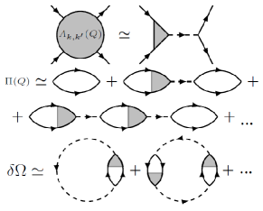
Figure 2: Local-field approximation: Feynman diagrams picture. Upper row: two-particle irreducible vertex in the particle-particle channel. Dashed line: exchange of a bare boson plus background interaction. Shaded triangle: renormalized vertex correction, depending on one frequency and one momentum. Central row: pairing susceptibility (3) as an RPA resummation of bubble diagrams connected by two-particle irreducible vertices. Lower row: RPA-like diagrams for the grand-canonical potential.

We obtain the same $\delta\Omega$ by the running-coupling constant method, after neglecting the intrinsic dependence of $\mathcal{G}$ on $g$ and $U_{bg}$. Thus, we expect this approximation to be quantitatively reliable for small to intermediate values of $g$ and $U_{bg}$. We then derive $\mu$ from

$$n=-\frac{\partial}{\partial\mu}(\Omega_{0}+\delta\Omega).$$ (7)

Eqs. (4)-(7) are the closed set describing the critical behavior in the crossover for narrow-to intermediate FF resonances. For their self-consistent solution, one iterates an initial guess for $\mathcal{G}$ (e.g. $\mathcal{G}=0$) until convergence.
Once discussed the essence of the theory, we now relax the $G_{0}$ approximation: we relate the scattering vertex $\Gamma=\left[\left(1-\mathcal{G}\right)U_{\text{eff}}\right]/\left[1-\left(1-\mathcal{G}\right)U_{\text{eff}}\Pi_{0}\right]$ to $\mathcal{G}$, the fermionic self-energy $\Sigma(K_{n})=\sum_{Q_{n}}\Gamma(Q_{n})G_{0}(Q_{n}-K_{n})$ to $\Gamma(Q_{n})$, then updating $G_{0}\to G=[G_{0}^{-1}-\Sigma]^{-1}$ and $\Pi_{0}\to\widetilde{\Pi}_{0}(Q_{n})=\sum_{K_{n}}G(Q_{n}-K_{n})G(K_{n})$ in the vertex expression, with $n=\sum_{K_{n}}G(K_{n})e^{i\omega_{n}0^{+}}$ and the $\mathcal{G}$ constant during the loop. Here, $Q_{n}=(\nu_{n},\mathbf{q})$ ($K_{n}=(\omega_{n},\mathbf{k})$) is the 4-vector with a bosonic (fermionic) Matsubara frequency. This the analogue of a GW approximation For an overview see Giuliani and Vignale (2005).
Limiting cases- Despite the equations complexity, we can extract relevant analytical limits. We first need to regularize the (otherwise diverging) non-interacting susceptibilities. This requires Kokkelmans et al. (2002); Ohashi and Griffin (2003b) to renormalize $U_{bg}$, $g$ and $\nu$ into $U_{R}$, $g_{R}$ and $\nu_{R}$, exactly as in the two-body problem SoM . From now on we drop, for simplicity, $U_{bg}$. In the BCS limit with $\nu_{R}\gg\varepsilon_{F}$ and $T_{c}\ll T_{F}$  (7) reads $\mu\simeq\varepsilon_{F}$, so that $T_{c}^{\text{BCS}}\simeq{8e^{\gamma-2}{\pi}^{-1}\,\varepsilon_{F}}\exp\left[-({2\nu_{R}-2\varepsilon_{F}})/({N(0)\tilde{g}^{2}})\right]$, where $N(0)$ is the density of states at $\varepsilon_{F}$ and $\tilde{g}^{2}\equiv g_{R}^{2}[1-\mathcal{G}(0,0)]$. It can be shown that $0<\mathcal{G}(0,0)<1$ if an RPA $S(\mathbf{q})$ is inserted in (4). Thus, at fixed $\nu_{R}$, the local field correction suppresses $T_{c}$ with respect to its mean-field value. This result is reminiscent of the celebrated Gor’kov and Melik-Barkhudarov (GMB) correction in one-channel calculations Gor’kov and Melik-Barkhudarov (1961), stating that in the BCS limit particle-hole processes suppress $T_{c}$ and superfluid gap by a factor $\simeq 2.2$ Pisani et al. (2018b). In our theory, these particle-hole corrections show up in the $g$ renormalization. Indeed, evaluating in the BCS limit $\nu_{R}\gg\varepsilon_{F}$ Strinati et al. (2018) the BF vertex diagram $\Lambda^{\text{BF}}_{\mathbf{k},\omega}(\mathbf{q},\Omega)$ to lowest order as in Fig. 3, we get:

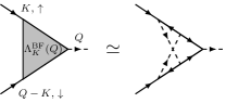
Figure 3: Lowest order contribution to the irreducible boson-fermion vertex $\Lambda^{\text{BF}}_{K}(Q)$, showing the coupling constant $g$ is renormalized by particle-hole processes (dashed lines are bare bosons).

$$\tilde{g}_{\text{GMB}}^{2}=g_{R}^{2}\left[1-\frac{g_{R}^{2}}{2\nu_{R}-2\varepsilon_{F}}N(0)\ln(4e)^{1/3}\right].$$ (8)

Replacing $g_{R}^{2}[1-\mathcal{G}]$ by $\tilde{g}_{\text{GMB}}^{2}$ in (6), $T_{c}$ results suppressed by $(4e)^{1/3}\simeq 2.2$. From the structure of our equations, using local field factors amounts to neglect the ($\mathbf{k}$, $\omega$) dependence in the full boson-fermion vertex $\Lambda^{\text{BF}}_{\mathbf{k},\omega}(\mathbf{q},\Omega)$, like in electron liquids For an overview see Giuliani and Vignale (2005). This defines the perimeter of our theory in capturing the $T_{c}$ suppression effects.
On the BEC limit with $\nu\ll-\varepsilon_{F}$, eq. (6) yields $\mu\simeq\nu$ and from (7) one obtains the BEC $T_{c}$ of $n/2$ bosons with mass $2m$: $T_{c}^{\text{BEC}}=({\pi}/{m})[{n}/({2\zeta(3/2)})]^{2/3}$.
Implications for current experiments- Self-consistent calculations in the narrow-resonance case with $k_{F}|r_{0}|\simeq 5$ in the BCS limit, yields a more limited suppression with our theory, so that $T_{c}$ is enhanced by a factor up to $\simeq 10\%$ than the (perturbative) $T_{c,\text{GMB}}$. The resonance turns out to be characterized by a maximum at $T_{c}$ Perali et al. (2004b), that reduces towards the narrow limit Bonetti et al. : in the broad resonance limit with $k_{F}r_{0}\simeq 0.5$ we get $T_{c}/T_{F}\simeq 0.22$, comparable with the QMC value $T_{c}/T_{F}=0.24(2)$ by Bulgac et al. Bulgac et al. (2006). At unitarity, varying the resonance width in the range $0.5<k_{F}|r_{0}|<5$ by one order of magnitude yields variations of the maximum $T_{c}$ up to $\simeq 8\%$ Bonetti et al. .
Conclusions- We have developed a unifying fully self-consistent theory of superfluidity with pairing fluctuations beyond mean field, hinging on the original Fano-Feshbach microscopic resonant mechanism. Our theory bridges the description of the BCS-BEC crossover from narrow to broad FF resonances, in a region so far devoided of simulational methods and largely unexplored by theoretical methods. We brush up the old-fashioned concept of local field, successfully developed in electron liquids, and demonstrate its so-far unexplored methodological power to access a complex phase diagram where density, spin, and amplitude/phase fluctuations of a superfluid order parameter can be treated on equal footing with only one physical approximation.
Intermediate resonance widths are becoming accessible by a new class of experiments, like with fermionic Er atoms Baier et al. (2018b), Fermi-Hubbard simulators Mazurenko et al. (2017), or Fermi-Bose mixtures Lercher, A.D. et al. (2011), that can provide a test-bed for our theory. A systematic study of relevant observables like $T_{c}$ and superfluid gap at $T\ll T_{c}$, requires a full numerical solution, that is under way Bonetti et al. . Effects up to $10\%$ found in $T_{c}$ with respect to the broad resonance case, open up unexplored physics. Interest is also building up on the equation of state in neutron stars, where observational data are compatible with $k_{F}a\simeq-13$ and $k_{F}|r_{0}|\simeq 2$, though on the fully different fm length scale Baym (2010).