Similarity Kernel and Clustering via Random Projection Forests

Abstract

Similarity plays a fundamental role in many areas, including data mining, machine learning, statistics and various applied domains. Inspired by the success of ensemble methods and the flexibility of trees, we propose to learn a similarity kernel called rpf-kernel through random projection forests (rpForests). Our theoretical analysis reveals a highly desirable property of rpf-kernel: far-away (dissimilar) points have a low similarity value while nearby (similar) points would have a high similarity, and the similarities have a native interpretation as the probability of points remaining in the same leaf nodes during the growth of rpForests. The learned rpf-kernel leads to an effective clustering algorithm—rpfCluster. On a wide variety of real and benchmark datasets, rpfCluster compares favorably to K-means clustering, spectral clustering and a state-of-the-art clustering ensemble algorithm—Cluster Forests. Our approach is simple to implement and readily adapt to the geometry of the underlying data. Given its desirable theoretical property and competitive empirical performance when applied to clustering, we expect rpf-kernel to be applicable to many problems of an unsupervised nature or as a regularizer in some supervised or weakly supervised settings.

Index terms— Similarity learning, distance metric learning, clustering, rpf-kernel, kernel methods, random projection forests

1 Introduction

Similarity measures how similar or closely related different objects are. It is a fundamental quantity that is relevant whenever a distance metric or a measure of relatedness is used. Our interest is when the similarity is explicitly used. A wide range of applications use the notion of similarity. In data mining, the answer to a database (or web) query is often formulated as similarity search [25, 31] where instances similar to the one in the query are returned. More general is the k-nearest neighbor search, which has applications in robotic route planning [42], face-based surveillance systems [55], anomaly detection [2, 16, 57] etc. In machine learning, the entire class of kernel methods [59, 37] rely on similarity or the similarity kernel. The similarity kernel is also an essential part of popular classifiers such as support vector machines [19], the broad class of spectral clustering algorithms [62, 54, 40, 65, 72], and various kernalized methods such as kernel PCA [58], kernel ICA [3], kernel CCA [32], kernel k-means [23] etc. Another important class of methods that use similarity is clustering ensemble [64, 70] which use the similarity to encode how different data points are related to each other in terms of clustering when viewed from many different clustering instances. Additionally, the similarity is used as a regularization term that incorporates some latent structures of the data such as the cluster [17] or manifold assumption [5] in semi-supervised learning, or as regularizing features that capture the locality of the data (i.e., which of the data points look similar) [74]. In statistics, the notion of similarity is also frequently used (a significant overlap with those used in machine learning). It has been used as a distance metric in situations where the Euclidean distance is no longer appropriate or the distance needs to be adaptive to the data, for example in nonparametric density estimation [9, 51] and intrinsic dimension estimation [11, 44]. Another use is to measure the relatedness between two random objects, such as the covariance matrix. It is also used as part of the aggregation engine to combine data from multiple sources [66] or multiple views [24, 69].

The benefit of adopting a similarity kernel is immediate. It encodes important property about the data, and allows a unified treatment of many seemingly different methods. Also one may take advantage of the powerful kernel methods. However, in many situations, one has to choose a kernel that is suitable for a particular application. It will be highly desirable to be able to automatically choose or learn a kernel that would work for the underlying data. In this paper, we explore a data-driven approach to learn a similarity kernel. The similarity kernel will be learned through a versatile tool that was recently developed—random projection forests (rpForests) [75].

rpForests is an ensemble of random projection trees (rpTrees) [20] with the possibility of projections selection during tree growth [75]. rpTrees is a randomized version of the popular kd-tree [7, 31], which, instead of splitting the nodes along coordinate-aligning axes, recursively splits the tree along randomly chosen directions. rpForests combines the power of ensemble methods [13, 14, 30, 70, 27] and the flexibility of trees. As rpForests uses randomized trees as its building block, accordingly it has several desired properties of trees. Trees are invariant with respect to monotonic transformations of the data. Trees-based methods are very efficient with a log-linear (i.e., $O(n\log(n))$) average computational complexity for growth and $O(\log(n))$ for search where $n$ is the number of data points. As trees are essentially recursive space partitioning methods [7, 20, 71], data points falling in the same tree leaf node would be close to each other or “similar”. This property is often leveraged for large scale computation [21, 48, 72, 75] etc. Now it forms the basis of our construction of the similarity kernel—data points in the same leaf node are likely to be similar and dissimilar otherwise. Additionally, as individual trees are rpTrees thus can adapt to the geometry of the data and readily overcomes the curse of dimensionality [20].

Ideally, for a similarity kernel, similar objects should have a high similarity value while low similarity value for dissimilar objects. Similarity as produced by a single tree may suffer from the undesirable boundary effect—similar data points may be separated into different leaf nodes during the growth of a tree. This will cause problem for a similarity kernel for which the similarity of every pair (or most pairs) of points matters. The ensemble nature of rpForests allows us to effectively overcome the boundary effect—by ensemble, data points separated in one tree may meet in another; indeed rpForests reduces the chance of separating nearby points exponentially fast [75]. Meanwhile, dissimilar or far-away points would unlikely end up in the same leaf node. This is because, roughly, the diameter of tree nodes keeps on shrinking during the tree growth, and eventually those dissimilar points would be separated if they are far away enough. Thus a similarity kernel produced by rpForests would possess the expected property.

Our main contributions are as follows. First, we propose a data-driven approach to learn a similarity kernel from the data by rpForests. It combines the power of ensemble and the flexibility of trees; the method is simple to implement, and readily adapt to the geometry of the data. As an ensemble method, easily it can run on clustered or multi-core computers. Second, we develop a theory on the property of the learned similarity kernel: similar objects would have high similarity value while low similarity value for dissimilar objects; the similarity values have a native interpretation as the probability of points staying in the same tree leaf node during the growth of rpForests. With the similarity kernel learned by rpForests, we develop a highly competitive clustering algorithm, rpfCluster, which compares favorably to spectral clustering and a state-of-the-art ensemble clustering method.

The remainder of this paper is organized as follows. In Section 2, we give a detailed description of how to produce a similarity kernel by rpForests and a clustering method based on the resulting similarity kernel. This is followed by a little theory on the similarity kernel learned by rpForests in Section 3. Related work are discussed in Section 4. In Section 5, we first provide examples to illustrate the desired property of the similarity kernel and its relevance in clustering, and then present experimental results on a wide variety of real datasets for rpfCluster and its competitors. Finally, we conclude in Section 6.

2 Proposed approach

In this section, we will first describe rpForests, and then discuss how to generate the similarity kernel with rpForests and to cluster with the similarity kernel, followed by a brief introduction to spectral clustering [62, 54, 40, 65].

2.1 Algorithmic description of rpForests

Our description of the rpForests algorithm is based on [75]. Each tree in rpForests is an rpTree. The growth of an rpTree follows a recursive procedure. It starts by treating the entire data as the root node and then split it into two child nodes according to a randomized splitting rule. On each child node, the same splitting procedure applies recursively until some stopping criterion is met, e.g., the node becomes too small (i.e., contains too few data points).

In rpTree, the split of a node is along a randomly generated direction, say $\stackrel{{\scriptstyle\rightharpoonup}}{{r}}$. Assume the node to split is $W$. There are many ways to split node $W$. One choice that is simple to implement is to select a point, say $c$, uniformly at random over the interval formed by the projection of all points in $W$ onto $\stackrel{{\scriptstyle\rightharpoonup}}{{r}}$, denoted by $W_{\stackrel{{\scriptstyle\rightharpoonup}}{{r}}}=\{P_{\stackrel{{\scriptstyle\rightharpoonup}}{{r}}}(x)=r\bm{\cdot}x:~{}x\in W\}$. The left child is given by $W_{L}=\{x\in W:P_{\stackrel{{\scriptstyle\rightharpoonup}}{{r}}}(x)<c\}$, and the right child $W_{R}$ by the rest of points. Another popular choice is to choose the median of $W_{\stackrel{{\scriptstyle\rightharpoonup}}{{r}}}$ as the split point. We empirically evaluate the performance of uniform random split and split by median, and found their difference to be rather small. Let $V=\{X_{1},...,X_{n}\}$ denote the given data set. Let $\mathcal{W}$ denote the set of nodes to be split (termed as the working set). Let $n_{s}$ denote a constant such that a node will not be split further if its size is smaller than $n_{s}$. Denote the rpForests by $\mathcal{F}$; assume there are totally $T$ trees. The algorithm for generating rpForests is described as Algorithm 1.

Algorithm 1   rpForests(V, T)

1:  Initialize $\mathcal{F}\leftarrow\emptyset$;

2:  for $i=1$ to $T$ do

3:     Let $V$ be the root node of tree $t_{i}$;

4:     Initialize the working set $\mathcal{W}\leftarrow\{V\}$;

5:     while $\mathcal{W}$ is not empty do

6:        Sample $W\in\mathcal{W}$ and update $\mathcal{W}\leftarrow\mathcal{W}\setminus\{W\}$;

7:        if $|W|<n_{s}$ then

8:           Skip to the next round of the loop;

9:        end if

10:        Generate a random direction $\stackrel{{\scriptstyle\rightharpoonup}}{{r}}$;

11:        Project $W$ onto $\stackrel{{\scriptstyle\rightharpoonup}}{{r}}$, $W_{\stackrel{{\scriptstyle\rightharpoonup}}{{r}}}=\{P_{\stackrel{{\scriptstyle\rightharpoonup}}{{r}}}(x):x\in W\}$;

12:        Sample splitting point $c$ uniformly at random from the interval $[\min(W_{\stackrel{{\scriptstyle\rightharpoonup}}{{r}}}),\max(W_{\stackrel{{\scriptstyle\rightharpoonup}}{{r}}})]$;

13:        Set $W_{L}\leftarrow\{x:P_{\stackrel{{\scriptstyle\rightharpoonup}}{{r}}}(x)<c\}$ and $W_{R}\leftarrow\{x:P_{\stackrel{{\scriptstyle\rightharpoonup}}{{r}}}(x)\geq c\}$;

14:        Split node $W$ by $W=W_{L}\cup W_{R}$;

15:        Update working set by $\mathcal{W}\leftarrow\mathcal{W}\cup\{W_{L},W_{R}\}$;

16:     end while

17:     Add tree $t_{i}$ to the ensemble $\mathcal{F}\leftarrow\mathcal{F}\cup\{t_{i}\}$;

18:  end for

19:  return($\mathcal{F}$);

Note that in choosing the splitting direction, we follow the basic implementation of rpForests as documented in [75] which would simply generate a random direction.

2.2 Similarity kernel and clustering

In this subsection, we will describe algorithms for the generation of a similarity kernel with rpForests and for clustering with the resulting similarity kernel.

Once rpForests is grown, the generation of the similarity kernel is fairly straightforward. For each tree, one scans through all the leaf nodes and collect information regarding if two points are in the same leaf node, and then aggregate such information from all trees in rpForests. For ease of description, let $S[A_{1},A_{2}]$ denote all entries in matrix $S$ with their position indexed by the Cartesian product $A_{1}\times A_{2}$ of two sets of integers $A_{1}$ and $A_{2}$. The generation of the similarity kernel is described as Algorithm 2. Note that here the notation, $\mathcal{N}$, for a node may also refer to the index of all points in this node for ease of description.

Algorithm 2   rpfSimilarity($\mathcal{F}$)

1:  Initialize a similarity matrix $S\leftarrow\bf{0}$;

2:  for each tree $t\in\mathcal{F}$ do

3:     for each leaf node $\mathcal{N}\in t$ do

4:        Increase the similarity count for each entry in $S[\mathcal{N},\mathcal{N}]$;

5:     end for

6:  end for

7:  Set $S\leftarrow S/(\mbox{number of trees in}~{}\mathcal{F})$;

8:  Return $S$;

The similarity matrix $S$ as produced by Algorithm 2 is a valid kernel matrix. This can be argued as follows. Let $S^{(t)}$ denote the similarity matrix generated by tree $t$. Then $S^{(t)}$ is a block diagonal matrix with all points in the same leaf node form a diagonal block of all entries 1, and all off-diagonal blocks are 0 as those correspond to points from different leaf nodes. Let matrix $M$ be one of the diagonal blocks in $S^{(t)}$. Then $M$ is positive semidefinite, as the following holds

$$z^{T}Mz=(z_{1}+z_{2}+\cdots+z_{m})^{2}\geq 0$$

for any vector $z=(z_{1},...,z_{m})$. This implies that matrix $S^{(t)}$ is positive semidefinite. It follows that the average matrix

$$S=\frac{1}{T}\sum_{t=1}^{T}S^{(t)}$$

is also positive semidefinite. Thus the similarity matrix $S$ produced by rpForests is a valid kernel matrix. Due to its intimate connection to rpForests, the resulting kernel is termed as rpf-kernel.

On rpf-kernel $S$, it is straightforward that one can apply spectral clustering to obtain a clustering of the original data. This is described as Algorithm 3.

Algorithm 3   rpfCluster($S$, K)

1:  Threshold similarity kernel by $S_{ij}\leftarrow 0$ if $S_{ij}<\beta_{1}$;

2:  $S\leftarrow exp(S/\beta_{2})$ for some bandwidth $\beta_{2}$;

3:  Apply spectral clustering to $S$ to get the cluster assignment;

Note that here we threshold the kernel $S$ following the same idea as [70]. This will help get rid of the spurious similarity between points in different clusters (in the ideal case, points from different clusters would have a 0 similarity if clustering is concerned). Also similar as in the practice of using the Gaussian kernel in various kernel methods, we apply a bandwidth to reflect the correct scale at which the data are clustered.

2.3 Spectral clustering

In this subsection, we will briefly describe spectral clustering since it is used in the last stage of rpfCluster and also as a competing algorithm in our experiments (c.f. Section 5.2.2). Spectral clustering works on the affinity graph $\mathcal{G}=(V,\mathcal{E})$ formed on the set of data points $V=\{X_{1},...,X_{n}\}$, where each vertex corresponds to a data point and the edge, $S_{ij}\in\mathcal{E}$, encodes the affinity (similarity) between data points $X_{i}$ and $X_{j}$. The matrix $S=(S_{ij})_{i,j=1}^{n}$ is called the affinity or similarity matrix.

There are several variants of spectral clustering [62, 54, 40]. In the present paper we adopt normalized cuts (Ncut) [62] for a concrete description (when the size of the dataset is big, e.g., larger than 2000, the Nystrom method [29] is used to compute the eigen-decomposition); other formulations are also possible. A graph cut between two sets of vertices, $V_{1},V_{2}\subset V$, is the collection of all edges crossing $V_{1}$ and $V_{2}$, and the size of the cut is defined by

$$\mathcal{E}(V_{1},V_{2})=\sum_{X_{i}\in V_{1},X_{j}\in V_{2}}S_{ij}.$$

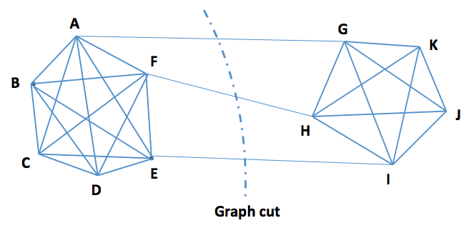
Figure 1: Illustration of a graph cut.

Figure 1 is an illustration of the graph cut. The dashed line cuts the graph into two partitions, $V_{1}=\{A,B,C,D,E,F\}$ and $V_{2}=\{G,H,I,J,K\}$. The total weights of three edges, $AG,FH,EI$, crossing $V_{1}$ and $V_{2}$ is the size of the cut. It is easy to see that the concept of graph cut can be extended to graph partitions that involve multiple sets. Spectral clustering aims to find a minimal normalized graph cut

$$\arg\min_{V_{1},...,V_{K}}\sum_{j=1}^{K}\frac{\mathcal{E}(V_{j},V)-\mathcal{E}(V_{j},V_{j})}{\mathcal{E}(V_{j},V)},$$ (1)

where $(V_{1},\ldots,V_{K})$ is a partition of $V$. Directly solving (1) is intractable as it is an integer programming problem, and spectral clustering is based on a relaxation of (1) into an eigenvalue problem. In particular, Ncut relaxes the indicator vectors (corresponding to cluster membership) with real values, resulting in a generalized eigenvalue problem.

Ncut computes the second eigenvector of the Laplacian of matrix $S$ to find a bipartition of the data. The nonnegative components of the eigenvector corresponds to one partition and the rest to the other. The same procedure is applied recursively until reaching the number of specified clusters.

3 Theoretical analysis

The growth of rpForests involves quite a bit of randomness, i.e., in the choice of splitting directions and the splitting point. A central concern would be the quality of the rpf-kernel learned by rpForests—will the learned similarity kernel preserve the true similarity values? Our analysis will ascertain that “far-away” (or dissimilar) points would have low similarity while high similarity for nearby (or similar) points. The behavior of nearby points under rpForests was analyzed in [75] which states that the probability that such points are separated during the growth of rpForests is small thus one would expect a high similarity among such points. Here we follow their analysis but focus on the behavior of far-away points, and, for tractability, we only consider the basic implementation of rpForests [75]. Note that here far-away or nearby are not precisely defined; a crude rule for nearby is that one point is a k-nearest neighbor of another while far-away is when the distance between two points is larger than a small constant, say $\alpha$, and both $k$ and $\alpha$ are application dependent. Throughout our analysis, we use the Euclidean distance; however, it should be clear that other properly defined distance metrics also apply.

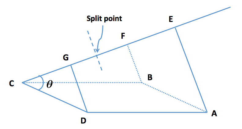
Figure 2: Illustration of the geometry involved in the random projection (image courtesy [75]). $A$ and $B$ are the two points of interest. Line $CE$ indicates the direction of random projection. $E$ and $F$ are the projection of points $A$ and $B$ onto line $CE$. Line $CD$ is parallel to $AB$, and $G$ is the projection of $D$ onto line $CE$. The split point will lie anywhere on line $CE$ within the range of of the projections of all points at a tree node.

We will use Figure 2 to assist our analysis. Assume $A$ and $B$ are the two points of interest, and let line $CE$ denote the direction of the random projection. We can conveniently assume that $C$ is the point of origin. Point $D$ is chosen such that $CD\parallel AB$ and that $|AB|=|CD|$ where $|.|$ denotes the length of a line segment and $\parallel$ indicates parallel. Assume $G,E,F$ are the points projected from $D,A,B$ onto $CE$, respectively. It was shown that $|CG|=|EF|$ in [75].

For a given point set $\Omega$, it can be cut along different directions. [75] considers a direction along which the data stretch the least (the size of such a stretch is called the neck size). Here we shall consider its counterpart which is defined as follows.

Definition. Let $\Omega$ be a set of points. Define the size of its principal stretch as

$$\rho(\Omega)=\sup_{\stackrel{{\scriptstyle\rightharpoonup}}{{r}}}\sup_{x_{1},x_{2}\in\Omega}\{\mid P_{\stackrel{{\scriptstyle\rightharpoonup}}{{r}}}(x_{1})-P_{\stackrel{{\scriptstyle\rightharpoonup}}{{r}}}(x_{2})\mid\}.$$

The neck size was used to bound the probability that nearby points stay unseparated under rpForests. In the following, we will state a result that characterizes the probability that far-away points would be separated under rpForests.

Theorem 3.1.

Let $\Omega$ be a set of points with a positive principal stretch, i.e., $\rho(\Omega)>0$. Given any two points, $A,B\in\Omega$, for a random projection defined by the rpTree,

$$P(\text{A and B separated by a random projection})\geq\frac{2d}{\pi\rho(\Omega)},$$

where $d$ denote the distance between points $A$ and $B$.

Proof.

The proof is based on the geometry illustrated in Figure 2. The main idea is to condition on the angle, $\theta$, between the random direction $CE$ and line $AB$. Note that this is also the angle between the random direction and $CD$ as lines $AB\parallel CD$. It is clear that $0\leq\theta\leq\pi/2$.

Given angle $\theta$, points $A$ and $B$ are separated if the splitting point is within their projections onto the random direction. That is, the randomly selected splitting point falls between $E$ and $F$. Let $L$ denote the size of the range of the projected points. That is,

$$L=\sup_{x_{1},x_{2}\in\Omega}\{\mid P_{\stackrel{{\scriptstyle\rightharpoonup}}{{r}}}(x_{1})-P_{\stackrel{{\scriptstyle\rightharpoonup}}{{r}}}(x_{2})\mid\}.$$

As the splitting point is chose uniformly at random along the random direction, the probability that $A$ and $B$ are split is given by $|EF|/L$. As $|EF|=|CG|=|AB|cos(\theta)$,

$$P(\text{A and B separated by a random projection})$$

$$= \int_{0}^{\pi/2}P\left(\text{A and B are separated}\mid\theta\right)\cdot\frac{2}{\pi}d\theta$$

$$= \int_{0}^{\pi/2}\frac{|AB|cos(\theta)}{L}\cdot\frac{2}{\pi}d\theta$$

$$\geq \frac{2|AB|}{\pi\rho(\Omega)}\int_{0}^{\pi/2}cos(\theta)d\theta=\frac{2d}{\pi\rho(\Omega)}.$$

∎

Now assume a tree $t$ in rpForests splits $J_{t}\in[J_{1},J_{2}]$ times, and the principal stretch of all the child nodes shrinks by a factor in the range of $[\gamma_{1},\gamma_{2}]\subset(0,1)$. Then, for any two far-away points, $A$ and $B$, the probability that they would be separated in tree $t$ can be estimated as follows.

$A$ and $B$ are separated if they are separated at any one of the node splits. Let $N_{t}^{(1)},N_{t}^{(2)},\cdots,N_{t}^{(J_{t})}$ indicate the collection of nodes in the growth of tree $t$ such that each node in the sequence is either the sibling or the descendent of proceeding nodes. Then

$$P(\text{A and B separated in tree $t$})$$

$$= P\left(\text{$\cup_{i=1}^{J_{t}}$ (A and B separated when splitting node $N_{t}^{(i)}$})\right)$$

$$\geq P(\text{A and B separated when splitting node $N_{t}^{(J_{t})}$}).$$

Now we can apply Theorem 3.1 to node $N_{t}^{(J_{t})}$, and get

$$P(\text{A and B separated in tree $t$})\geq\frac{2d_{AB}}{\pi\rho(N_{t}^{(J_{t})})}\geq\frac{2d_{AB}}{\pi\rho\gamma_{2}^{J_{1}-1}}$$ (2)

where $\rho$ is the size of the principal stretch over the entire data. One implication of (2) is that as the enclosing node shrinks, eventually two far-away points will be separated in probability. Under similar conditions, the result established in [75] implies that, for nearby points $A$ and $B$,

$$P(\text{A and B separated in tree $t$})\leq\frac{2d_{AB}}{\pi\nu}\frac{1}{\gamma_{1}^{J_{2}-2}(1-\gamma_{1})}$$ (3)

where $\nu$ is the neck size of the entire data. Bound (3) indicates that the probability of separation for “nearby” points remains small in tree $t$, since the near neighbor distance decreases very quickly for large set of data [11, 56]. Bounds (2) and (3) will allow us to characterize important properties of the similarity kernel learned by rpForests.

Now let us consider the similarity value for points $A$ and $B$ in the rpf-kernel produced by rpForests which consists of $T$ trees. For $j=1,2,...,T$, define indicator random variables

$$\mathbb{I}_{j}~{}=\left\{\begin{array}[]{ll}1,&~{}\mbox{if A and B separated in j-th tree}{}\\ 0,&~{}\mbox{otherwise.}\end{array}\right.$$

Then $\mathbb{I}_{j}$’s are independent and of the same distribution conditional on the data. Thus $\Delta=\mathbb{I}_{1}+\mathbb{I}_{2}+...+\mathbb{I}_{T}$ gives the number of trees for which $A$ and $B$ are separated. It is clear that $\Delta$ follows a binomial distribution or is approximately normal if $T$ is large. Assume $\mathbb{I}_{j}$ has a mean $\mu$ and standard deviation $\sigma$. For “far-away” points $A$ and $B$, we wish to show that, with high probability, their similarity is smaller than a small value (not arbitrary small), say $\delta$. We have the following normal approximation

$$P(\mbox{$A$ and $B$ have a similarity at most $\delta$})$$ (4)

$$= P(\Delta\geq(1-\delta)T)$$

$$\approx P(Z\geq(1-\delta-\mu)\sqrt{T}/\sigma)$$

where $Z$ is the standard normal random variable. We wish to argue that $1-\delta-\mu<0$ for some small $\delta>0$. Then, if $T$ is large, the probability in (4) will be high since then $(1-\delta-\mu)\sqrt{T}/\sigma$ will be very far towards $-\infty$. By (2),

$$\mu=P(\mbox{$A$ and $B$ separated in a tree})\geq 2d_{AB}/(\pi\rho\gamma_{2}^{J_{1}-1}).$$ (5)

If the number of data points $n$ increases, then the number of splits $J$ will also increase. As long as the principal stretch size of the nodes shrinks steadily, that is, $\gamma_{2}$ is strictly less than 1. Thus $\mu$ will be close to 1, and would satisfy $1-\delta-\mu<0$ for far-away points $A$ and $B$. Therefore, with high probability, the similarity of far-away points $A$ and $B$ will stay below some small $\delta$.

For nearby points $A$ and $B$, we can follow a similar argument, i.e., (3), and conclude that, with high probability, their similarity will be large. Thus, we have argued that the rpf-kernel produced by rpForests has the desirable property: far-away (dissimilar) points have low similarity while high similarity for nearby (similar) points. In Section 5.1 we will provide a toy example to demonstrate such a property.

4 Related work

Similarity plays a very important role in machine learning. Due to the intimate connection between similarity and metric learning, we do not distinguish the two in this section. A simple similarity measure is typically defined through a closed-form function such as the cosine (or weighted cosine along principal directions [61]), Euclidean (or Minkoski) distance function etc. More sophisticated is the bilinear similarity which measures the similarity of any two objects $x_{1},x_{2}\in\mathbb{R}^{p}$ by a bilinear form

$$f_{S}(x_{1},x_{2})=(x_{1}-x_{2})^{T}S(x_{1}-x_{2})$$

where $S$ is a symmetric positive semidefinite matrix. This allows to incorporate feature weights or feature correlations into the similarity, and the Mahalanobis distance [1] is a classic example. Indeed many research in similarity learning starts from an early work on learning the Mahalanobis distance with side information such as examples of similar pairs of objects [68]. There are many followup work along this line, for example, [60] regularizes the learning by large margin, [4] uses side-information in the form of equivalence constraints, [34] attempts to optimize leave-one-out error of a stochastic nearest neighbor classifier, [22] minimizes the relative entropy between two Gaussians under constraints on the distance function, [67] learns a large-margin nearest neighbor metric such that k-nearest neighbors are of the same class while different classes otherwise. Later work either adds more constraints (such as sparsity) or extends the Mahalanobis metric, or on broader classes of problems (such as ranking); this includes [18, 36, 46, 49, 47, 39]. Similarity or metric learning is a big topic, and it is beyond our scope to have a more thorough review on existing work; readers can refer to surveys [76, 43, 6, 53] and references therein. Existing work are almost exclusively supervised or weakly supervised in nature, our work is different in that it is unsupervised.

Another related topic is clustering ensemble [64, 33, 8, 70]. Clustering ensemble works by first generating many clustering instances, and then produce the final cluster by aggregating results from individual clustering instances. Literature on clustering ensemble is huge; readers can refer to [64, 26, 70, 12] and references therein. Clustering ensemble is related as each tree in rpfCluster can be viewed as an instance of clustering where points in the same leaf node form a cluster. Most closely related are random projection based clustering ensemble [26] and Cluster Forests (CF) [70]. [26] generates individual clustering instances by random projection of the original data onto some low dimensional space and then perform clustering. rpfCluster differs by generating a clustering instance through the growth of a tree which iteratively refines the clustering, or, rpfCluster projects the data onto low dimensional spaces by a series of random projections with each to a one-dimension space. Same as rpfCluster, CF also iteratively improves clustering instances, and produces the final cluster by spectral clustering on the learned similarity kernel; the difference is that CF generates clustering instances by a base clustering algorithm and refines each clustering instances by randomized feature pursuits.

Finally there are connections to Random Forests (RF) [14]. Both RF and rpfCluster generates ensemble of trees with random ingredients; the difference is that RF is supervised as tree growth is guided by class labels while rpfCluster grows trees unsupervisedly, also RF splits on coordinates while rpfCluster on random projections. Both rpfCluster and CF can be viewed as unsupervised extensions to RF. CF aims at clustering by ensemble of iteratively refined clustering instances through randomized feature pursuits (see also [10]) while rpfCluster learns the similarity kernel by ensemble of random projection trees. Another connection is that RF can run in unsupervised mode [14, 63] to learn a suitable distance metric for clustering; this is done by synthesizing a contrast pattern through randomization of the original data by randomly permuting the data along each of its features thus breaking the covariance structure of the data (implemented by the proximity option in the R package “randomForest”), which is fundamentally different from our approach.

5 Experiments

Our experiments consists of two parts. In the first part, we will give illustrative examples to help the readers better appreciate the desired property of the rpf-kernel learned by rpForests, and its relevance for clustering. In the second part, we evaluate the empirical clustering performance of rpfCluster and compare it to three competing clustering algorithms, including K-means clustering [35] as the baseline, the NJW algorithm [54] as a popular implementation of spectral clustering, and CF [70] as state-of-the-art ensemble clustering algorithm, on a wide variety of real datasets. The two parts are presented in Section 5.1 and Section 5.2, respectively.

5.1 Illustrative examples

In this section, we will provide two illustrative examples. One serves to illustrate the desired property of similarity kernel learned by rpForests, and the other to demonstrate the propagation of similarity through points in the same cluster.

5.1.1 Example on similarity kernel

To appreciate the desirable property of the rpf-kernel produced by rpForests, we will use a popular yet simple dataset, the Iris flower data. It was introduced by one of the founders of modern statistics, R. A. Fisher, in 1936 [28] for discriminant analysis, and has since become one of the most widely used datasets. The data consist of three species of Iris, Iris setosa, Iris versicolor, and Iris virginica, with 50 instances each on four features, the length and width of the sepals and petals, respectively.

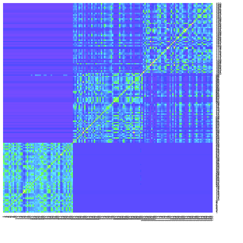
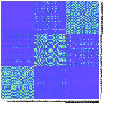
Figure 3: Heatmap of the similarity matrix generated by the Gaussian kernel (left) and by rpForests (right), respectively.

Figure 3 shows the heatmap of the similarity matrix generated by the Gaussian kernel and by rpForests, respectively. It can be seen that, in both cases, the similarity between data points in the same species (i.e., the diagonal blocks) are higher than otherwise. In particular, the similarities are close to 0 between the Iris setosa and the Iris virginica. This is expected. However, the contrast between other diagonal and non-diagonal blocks by rpForests is much sharper than those by the Gaussian kernel. We attribute this to the Gaussian kernel as a sole function of the distance between points which is Euclidean and every feature is equally weighted, and further the potential smoothing effect of the Gaussian kernel. In contrast, the kernel formed by rpForests would be a result of both the distance between points and their neighborhood thus is able to take advantage of the geometry in the data. Further work is being conducted to understand these.

We then run spectral clustering algorithm on the rpf-kernel generated by rpForests, and obtain a clustering and co-cluster accuracy (see definition in Section 5.2.1) of 96.67% and 94.95%, respectively. This is at the level of classification by some best classifiers such as RF despite that rpfCluster is unsupervised learning. The clustering and co-cluster accuracy on the Gaussian kernel are noticeably inferior, which are 92.00% and 90.55%, respectively.

5.1.2 Example on clustering

When adopting the rpf-kernel produced by rpForests for clustering, one might notice that two points in the same cluster may have a low similarity (even though rpf-kernel is able to pick up structural information from the data) if they are far away from each other (since these two points are far away, likely they would be put into different leaf nodes by rpForests thus a low value of similarity in the resulting similarity kernel); for example, two points that are located at the opposite ends of the cluster. However, this will not cause a problem for the subsequent spectral clustering which is built on local similarity. One empirical evidence is various algorithms for the speeding up of spectral clustering by sparsifying the similarity matrix based on k-nearest neighbors where similarity between non-kNNs are truncated to be 0.

Here we supply a simple numerical example for illustration: far-away points will not be assigned to different clusters by spectral clustering as long as they are inside a region where all points has high similarity to their near neighbors. Assume there are 9 points, $X_{1-9}$, on a line which form two clusters, $X_{1-4}$ and $X_{5-9}$, respectively. Assume, for each point, only its immediate neighbors have a non-zero similarity; further assume the similarity between $X_{4}$ and $X_{5}$ (from different clusters) is 0.3. The similarity matrix is given by

$$\small A=\left[\begin{array}[]{cccc;{2pt/2pt}ccccc}1.0&0.9&0.0&0.0&0.0&0.0&0.0&0.0&0.0\\ 0.9&1.0&0.9&0.0&0.0&0.0&0.0&0.0&0.0\\ 0.0&0.9&1.0&0.9&0.0&0.0&0.0&0.0&0.0\\ 0.0&0.0&0.9&1.0&0.3&0.0&0.0&0.0&0.0\\ \hdashline[2pt/2pt]0.0&0.0&0.0&0.3&1.0&0.9&0.0&0.0&0.0\\ 0.0&0.0&0.0&0.0&0.9&1.0&0.9&0.0&0.0\\ 0.0&0.0&0.0&0.0&0.0&0.9&1.0&0.9&0.0\\ 0.0&0.0&0.0&0.0&0.0&0.0&0.9&1.0&0.9\\ 0.0&0.0&0.0&0.0&0.0&0.0&0.0&0.9&1.0\end{array}\right]\normalsize$$

The eigenvector used for spectral clustering (normalized cuts [62]) is given by

$$[0.340~{}0.469~{}0.392~{}0.219~{}-0.098~{}-0.249~{}-0.351~{}-0.419~{}-0.304]^{T},$$

which gives the expected clustering, i.e., positive components correspond to one cluster and the rest the other cluster.

5.2 Experiments on real datasets

A wide range of real data are used for performance assessment. This includes 11 benchmark datasets taken from the UC Irvine Machine Learning Repository [45], namely, Soybean, SPECT Heart, image segmentation (ImgSeg), Heart, Wine, Wisconsin breast cancer (WDBC), robot execution failure (lp5), Madelon, Musk, Naval Plants, and the Magic Gamma (mGamma) dataset, as well as a remote sensing dataset (RS) [73], totally 12 datasets. For WDBC, it is standardized on its {5, 6, 25, 26}-th features; the Wine dataset is standardized on its {6, 14}-th features; for the Naval Plants data, we treat any record of measurements as requiring maintenance if both the q3Compressor and q3Turbine variables are above their median values thus converting the original numerical values into categorical labels. A summary of the datasets is given in Table 1. Note that all datasets come with labels. We made such a choice by recognizing that the ultimate goal of clustering is to get the membership of all the points right; many existing metrics for evaluating clustering algorithms are often a surrogate of this due to the lack of true labels. We will compare the performance by rpfCluster and three competing algorithms on two different performance metrics.

Dataset	Features	Classes	#Instances
Soybean	35	4	47
SPECT	22	2	267
ImgSeg	19	7	2100
Heart	13	2	270
Wine	13	3	178
WDBC	30	2	569
Robot	90	5	164
Madelon	500	2	2000
RS	56	7	3303
Musk	166	2	6598
NavalPlants	16	2	11934
mGamma	10	2	19020

Table 1: A summary of datasets.

5.2.1 Performance metrics

Two different performance metrics are used; these are adopted from [70]. One is the clustering accuracy, and the other is the co-cluster accuracy. Having different performance metrics allows to assess a clustering algorithm from different perspectives since one metric may favor certain aspects while overlooking others. Using the clustering or co-cluster accuracy has the advantage of closely aligning to the ultimate goal of clustering—assigning data points to proper groups—while other metrics are often a surrogate of the cluster membership. In the following, we formally define the two performance metrics.

Definition. Let $\mathcal{L}=\{1,2,...,l\}$ denote the set of class labels, and $h(.)$ and $\hat{h}(.)$ the true label and the label obtained by a clustering algorithm, respectively. The clustering accuracy is defined as

$$\rho_{c}(\hat{h})=\max_{\tau\in\Pi_{\mathcal{L}}}\left\{\frac{1}{n}\sum_{i=1}^{n}\mathbb{I}\{\tau\left(h(X_{i})\right)=\hat{h}(X_{i})\}\right\},$$ (6)

where $\mathbb{I}$ is the indicator function and $\Pi_{\mathcal{L}}$ is the set of all permutations on the label set $\mathcal{L}$. It measures the fraction of labels given by a clustering algorithm that agree with the true labels (or labels come with the dataset; we call these generally as reference labels for simplicity of description) up to a permutation of the labels. This is a natural extension of the classification accuracy (under 0-1 loss) and has been used by many work in clustering [68, 52, 72].

Definition. The co-cluster accuracy is defined by

$$\rho_{r}=\frac{\mbox{Number of correctly clustered pairs}}{\mbox{Total number of pairs}}$$

where by correctly clustered pair we mean two data points, determined to be in the same cluster by a clustering algorithm, are also in the same cluster according to the reference labels. Both the clustering accuracy and the co-cluster accuracy are converted to a scale of 100%.

5.2.2 Competing methods

We compare rpfCluster to three other clustering algorithms—K-means clustering, the NJW algorithm, and CF. Among these, K-means clustering is one of the most widely used clustering algorithms, NJW is a popular implementation of spectral clustering (commonly acknowledged as the class of best clustering algorithms), and CF is a state-of-the-art clustering ensemble algorithm. The comparison can also be viewed on different similarity kernels. The similarity kernel in CF is learned by randomized feature pursuits in individual clustering instances and then aggregate. In NJW, the Gaussian kernel is used by default. For the rest of this section, we will briefly describe K-means clustering, NJW and CF followed by a description on their implementations and parameters.

$K$-means clustering [35, 50] seeks to find a partition of the data into $K$ subsets $S_{1},S_{2},...,S_{K}$ such that the within-cluster sum of squares is minimized. Directly solving the problem is NP-hard. It is often implemented by an iteration of a two-step procedure. Starting with a set of randomly chosen initial cluster centroids, it iterates between: 1) assigning all the data points to their closest centroid (data points associated with the same centroid forms a cluster); and 2) recalculating the cluster centroid for data points in the same cluster, until the changes in the within-cluster sum of squares is small. Such a procedure would converge to local optima, and repeating this procedure for a number of times typically leads to fairly satisfactory results. K-means clustering is widely used in practice, as it is simple to implement and computationally fast.

The NJW algorithm [54] is a popular variant of spectral clustering. It works on the eigen-decomposition of the Laplacian of the similarity matrix over the data; the Gaussian kernel is used in the similarity measure which is defined as

$$S_{ij}=exp(-||X_{i}-X_{j}||^{2}/(2\sigma^{2})),$$

where $\sigma$ is the bandwidth. Then it embeds the original data points into a space spanned by the top few eigenvectors, followed by a normalization of the resulting embedding to the unit sphere. K-means clustering is then performed to get the cluster membership assignment.

As mentioned in Section 4, CF [70] is a clustering ensemble algorithm. Each clustering instance in CF is generated by randomized feature pursuit according to the $\kappa$ criterion [70] which is the ratio of the within-cluster and between-cluster sum of squared distances. It starts with a randomly selected features, then generates several sets of candidate features to run by a base clustering algorithm (e.g., K-means clustering as implemented in [70]) and keep the set of features that lead to the maximum decreases in the $\kappa$ value. This procedure is repeated until changes to the $\kappa$ value become too small. On each clustering instance a co-cluster indicator matrix is calculated, and the indicator matrices are then averaged to get the similarity matrix. Then similar steps as rpfCluster are executed to get the final clustering assignment. For details about its parameter settings, please refer to [70] from which we also adopt some experimental results in our comparison.

For $K$-means clustering, the R package kmeans() was used with the “Hartigan-Wong” [35] initialization, and the two parameters $(n_{it},n_{rst})$, which stands for the maximum number of iterations and the number of restarts during each run, respectively, are set to be $(1000,100)$. For NJW, function specc() of the R package “kernlab” [41] was used with the Gaussian kernel and an automatic search of the local bandwidth parameters. The number of trees in rpForests are chosen from $\{200,400,600\}$ and the difference in results is very small, the node splitting constant $n_{s}$ is $30$ except for $12$ for Soybean and $200$ for Madelon, the threshold level $\beta_{1}$ is chosen from $\{0,0.1,0.2,0.3,0.4\}$, and the step size for the search of bandwidth $\beta_{2}$ is 0.01 within (0,1] while 0.1 over (1,200].

5.2.3 Experimental results

The evaluation is based on two different performance metrics for, $\rho_{c}$ and $\rho_{r}$, as defined in Section 5.2.1. The results under $\rho_{c}$ and $\rho_{r}$ are shown as Figure 4 and Figure 5, respectively.

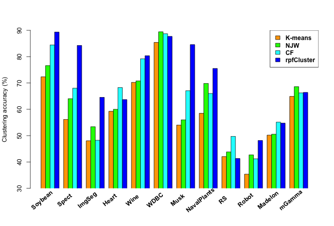
Figure 4: Comparison between K-means clustering, spectral clustering (NJW), CF, and rpfCluster for clustering accuracy $\rho_{c}$.

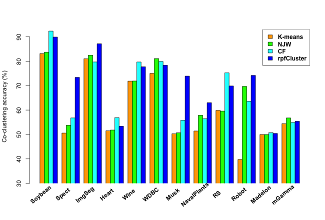
Figure 5: Comparison between K-means clustering, spectral clustering (NJW), CF, and rpfCluster for co-clustering accuracy $\rho_{r}$.

On all but two of the 12 datasets, either rpfCluster or CF is leading with rpfCluster having an edge. Under clustering accuracy $\rho_{c}$, rpfCluster is leading on 7 datasets, and ranks the second on 3 datasets while CF leads on 3 and seconds on 5. For co-cluster accuracy $\rho_{r}$, rpfCluster leads on 5 datasets and seconds on 6 while CF leads on 5 and seconds on 3. Overall, rpfCluster outperforms CF (also NJW and K-means clustering) on both two performance metrics.

6 Conclusions

We have proposed an effective approach for the unsupervised learning of a similarity kernel by rpForests. Our approach combines the power of ensemble methodology and the flexibility of trees. It is simple to implement, and readily adapt to the geometry of the underlying data. Our theoretical analysis reveals highly desirable property of the learned rpf-kernel: far-away points have low similarity while high similarity for nearby points, and the similarities have a native interpretation as the probability of points staying in the tree leaf nodes during the growth of rpForests. The learned rpf-kernel is readily incorporated into our clustering algorithm rpfCluster. On a wide variety of real and benchmark datasets, rpfCluster compares favorably to spectral clustering and a state-of-the-art clustering ensemble algorithm. Given the desirable theoretical property and the highly competitive empirical performance on clustering, we expect rpf-kernel to be applicable to other problems of an unsupervised nature or as a regularizer in supervised or weakly supervised settings. As each projection during the tree growth can be viewed as a coordinate, effectively rpForests is exploring some low dimensional manifolds (of a dimension approximately $O(\log(n))$) in high dimensional data, thus we expect rpForests to be also useful in manifold learning [15, 38].

References

- [1] T. W. Anderson. An Introduction to Multivariate Statistical Analysis. John Wiley & Sons, 1958.
- [2] F. Angiulli and C. Pizzu. Fast outlier detection in high dimensional spaces. Lecture Notes in Computer Science, 2431:43–78, 2002.
- [3] F. Bach and M. I. Jordan. Kernel independent component analysis. Journal of Machine Learning Research, 3:1–48, 2003.
- [4] A. Bar-Hillel, T. Hertz, N. Shental, and D. Weinshall. Learning a Mahalanobis metric from equivalence constraints. Journal of Machine Learning Research, 6:937–965, 2005.
- [5] M. Belkin, P. Niyogi, and V. Sindhwani. Manifold regularization: A geometric framework for learning from labeled and unlabeled examples. Journal of Machine Learning Research, 7:2399–2434, 2006.
- [6] A. Bellet, A. Habrard, and M. Sebban. A survey on metric learning for feature vectors and structured data. arXiv:1306.6709.v4, 2014.
- [7] J. Bentley. Multidimensional binary search trees used for associative searching. Communications of the ACM, 18(9):509–517, 1975.
- [8] A. Bertoni and G. Valentini. Ensembles based on random projections to improve the accuracy of clustering algorithms. In Proceedings of the 16th Italian conference on Neural Nets, pages 31–37, 2005.
- [9] P. J. Bickel and L. Breiman. Sums of functions of nearest neighbor distances, moment bounds, limit theorems and a goodness of fit test. The Annals of Probability, 11(1):185–214, 1983.
- [10] P. J. Bickel, G. Kur, and B. Nadler. Projection pursuit in high dimensions. Proceedings of the National Academy of Sciences, U. S. A., 115(37):9151–9156, 2018.
- [11] P. J. Bickel and D. Yan. Sparsity and the possibility of inference. Sankhya: The Indian Journal of Statistics, Series A (2008-), 70(1):1–24, 2008.
- [12] T. Boongoen and N. Iam-On. Cluster ensembles: A survey of approaches with recent extensions and applications. Computer Science Review, 28:1–25, 2018.
- [13] L. Breiman. Bagging predicators. Machine Learning, 24(2):123–140, 1996.
- [14] L. Breiman. Random Forests. Machine Learning, 45(1):5–32, 2001.
- [15] L. Cayton. Algorithms for manifold learning. Technical Report CS2008-0923, Department of Computer Science, UC San Diego, 2008.
- [16] V. Chandola, A. Banerjee, and V. Kumar. Anomaly detection: A survey. Technical Report, University of Minnesota, 2007.
- [17] O. Chapelle, J. Weston, and B. Schölkopf. Cluster kernels for semi-supervised learning. In Advances in Neural Information Processing Systems 15, pages 601–608, 2003.
- [18] G. Chechik, V. Sharma, U. Shalit, and S. Bengio. Large scale online learning of image similarity through ranking. Journal of Machine Learning Research, 11:1109–1135, 2010.
- [19] C. Cortes and V. N. Vapnik. Support-vector networks. Machine Learning, 20(3):273–297, 1995.
- [20] S. Dasgupta and Y. Freund. Random projection trees and low dimensional manifolds. In Fortieth ACM Symposium on Theory of Computing (STOC), 2008.
- [21] S. Dasgupta and K. Sinha. Randomized partition trees for nearest neighbor search. Journal Algorithmica, 72(1):237–263, 2015.
- [22] J. Davis, B. Kulis, P. Jain, S. Sra, and I. S. Dhillon. Information-theoretic metric learning. In Proceedings of the 24th International Conference on Machine Learning, pages 209–216, 2007.
- [23] I. Dhillon, Y. Guan, and B. Kulis. Kernel k-means: spectral clustering and normalized cuts. In Proceedings of the tenth ACM international conference on Knowledge discovery and data mining (SIGKDD), 2004.
- [24] Z. Ding, M. Shao, and Y. Fu. Robust multi-view representation: A unified perspective from multi-view learning to domain adaption. In Proceedings of 27th International Joint Conference on Artificial Intelligence, pages 5434–5440, 2018.
- [25] W. Dong, C. Moses, and K. Li. Efficient k-nearest neighbor graph construction for generic similarity measures. In Proceedings of the 20th International Conference on World Wide Web, 2011.
- [26] X. Z. Fern and C. E. Brodley. Random projection for high dimensional data clustering: A cluster ensemble approach. In Proceedings of the 20th International Conference on Machine Learning (ICML), 2003.
- [27] A. Feuerverger, Y. He, and S. Khatri. Statistical significance of the netflix challenge. Statistical Science, 27(2):202–231, 2012.
- [28] R. A. Fisher. The use of multiple measurements in taxonomic problems. Annals of Eugenics, 7(2):179–188, 1936.
- [29] C. Fowlkes, S. Belongie, F. Chung, and J. Malik. Spectral grouping using the Nystrm method. IEEE Transactions on Pattern Analysis and Machine Intelligence, 26(2):214–225, 2004.
- [30] Y. Freund and R. Schapire. Experiments with a new boosting algorithm. In International Conference on Machine Learning (ICML), 1996.
- [31] J. Friedman, J. Bentley, and R. Finkel. An algorithm for finding the best matches in logarithmic expected time. ACM Transactions on Mathematical Software, 3(3):209–226, 1977.
- [32] K. Fukumizu, F. Bach, and A. Gretton. Statistical consistency of kernel canonical correlation analysis. Journal of Machine Learning Research, 8:361–383, 2007.
- [33] A. Gionis, H. Mannila, and P. Tsaparas. Cluster aggregation. In the 21st International Conference on Data Engineering (ICDE), 2005.
- [34] J. Goldberger, G. E. Hinton E, S. Roweis, and R. Salakhutdinov. Neighbourhood components analysis. In Advances in Neural Information Processing Systems 17, pages 513–520, 2005.
- [35] J. A. Hartigan and M. A. Wong. A K-means clustering algorithm. Applied Statistics, 28(1):100–108, 1979.
- [36] M. Hirzer. Large scale metric learning from equivalence constraints. In Proceedings of the 2012 IEEE Conference on Computer Vision and Pattern Recognition (CVPR), pages 2288–2295, 2012.
- [37] T. Hofmann, B. Schlkopf, and A. Smola. Kernel methods in machine learning. The Annals of Statistics, 36(3):1171–1220, 2008.
- [38] X. Huo, X. Ni, and A. Smith. A survey of manifold-based learning methods. Recent Advances in Data Mining of Enterprise Data, pages 691–745, 2007.
- [39] Z. Kang, C. Peng, and Q. Cheng. Kernel-driven similarity learning. Neurocomputing, 267(C):210–219, 2017.
- [40] R. Kannan, S. Vempala, and A. Vetta. On clusterings: Good, bad and spectral. Journal of the ACM, 51(3):497–515, 2004.
- [41] A. Karatzoglou, A. Smola, and K. Hornik. kernlab: Kernel-based Machine Learning Lab. http://cran.r-project.org/web/packages/kernlab/index.html, 2013.
- [42] M. Kleinbort, O. Salzman, and D. Halperin. Efficient high-quality motion planning by fast all-pairs r-nearest-neighbors. In IEEE International Conference on Robotics and Automation (ICRA), pages 2985–2990, 2015.
- [43] B. Kulis. Metric Learning: A Survey. Foundations and Trends in Machine Learning, 5(4):287–364, 2015.
- [44] E. Levina and P. J. Bickel. Maximum likelihood estimation of intrinsic dimension. In Advances in Neural Information Processing Systems 17, 2005.
- [45] M. Lichman. UC Irvine Machine Learning Repository. http://archive.ics.uci.edu/ml, 2013.
- [46] D. Lim and G. Lanckriet. Efficient learning of mahalanobis metrics for ranking. In Proceedings of the 13rd International Conference on Machine Learning (ICML), 2014.
- [47] K. Liu, A. Bellet, and F. Sha. Similarity learning for high-dimensional sparse data. In International Conference on Artificial Intelligence and Statistics (AISTATS), 2015.
- [48] T. Liu, A. Moore, A. Gray, and K. Yang. An investigation of practical approximate nearest neighbor algorithms. In Neural Information Processing Systems (NIPS), volume 19, pages 825–832, 2004.
- [49] W. Liu, C. Mu, R. Ji, S. Ma, J. R. Smith, and S.-F. Chang. Low-rank similarity metric learning in high dimensions. In Proceedings of the 29-th AAAI Conference on Artificial Intelligence, pages 2792–2799, 2015.
- [50] S. P. Lloyd. Least squares quantization in PCM. IEEE Transactions on Information Theory, 28(1):128–137, 1982.
- [51] Y. P. Mack and M. Rosenblatt. Multivariate k-nearest neighbor density estimates. Journal of Multivariate Analysis, 9:1–15, 1979.
- [52] M. Meila, S. Shortreed, and L. Xu. Regularized spectral learning. Technical report, Department of Statistics, University of Washington, 2005.
- [53] P. Moutafis, M. Leng, and I. A. Kakadiaris. An overview and empirical comparison of distance metric learning methods. IEEE Transactions on Cybernetics, 47(3):612–625, 2017.
- [54] A. Y. Ng, M. I. Jordan, and Y. Weiss. On spectral clustering: analysis and an algorithm. In Neural Information Processing Systems (NIPS), volume 14, 2002.
- [55] C. Otto, D. Wang, and A. K. Jain. Clustering millions of faces by identity. arXiv:1604.00989, 2016.
- [56] M. Penrose and J. Yukich. Laws of large numbers and nearest neighbor distances. Advances in Directional and Linear Statistics, pages 189–199, 2010.
- [57] S. Ramaswamy, R. Rastogi, and K. Shim. Efficient algorithms for mining outliers from large data sets. In Proceedings of the ACM SIGMOD, pages 427–438, 2000.
- [58] B. Schlkopf. Nonlinear component analysis as a kernel eigenvalue problem. Neural Computation, 10:1299–1319, 1998.
- [59] B. Schlkopf and A. Smola. Learning with kernels: Support Vector Machines, Regularization, Optimization, and Beyond. MIT Press, 2001.
- [60] M. Schultz and T. Joachims. Learning a distance metric from relative comparisons. In Advances in Neural Information Processing Systems (NIPS), 2003.
- [61] C. Shahabi and D. Yan. Real-time pattern isolation and recognition over immersive sensor data streams. In Proceedings of the 9th International conference on multi-media modeling, pages 93–113, 2003.
- [62] J. Shi and J. Malik. Normalized cuts and image segmentation. IEEE Transactions on Pattern Analysis and Machine Intelligence, 22(8):888–905, 2000.
- [63] T. Shi and S. Horvath. Unsupervised learning with random forest predictors. Journal of Computational and Graphical Statistics, 15(1):118–138, 2006.
- [64] A. Strehl and J. Ghosh. Cluster ensembles – a knowlwdge reuse framework for combining multiple partitions. Journal of Machine Learning Research, 3:582–617, 2002.
- [65] U. von Luxburg. A tutorial on spectral clustering. Statistics and Computing, pages 395–416, 2007.
- [66] B. Wang, A. Mezlini, F. Demir, M. Fiume, Z. Tu, M. Brudno, B. Haibe-Kains, and A. Goldenberg. Similarity network fusion for aggregating data types on a genomic scale. Nature Methods, 11:333–337, 2014.
- [67] K. Q. Weinberger and L. K. Saul. Distance metric learning for large margin nearest neighbor classification. Journal of Machine Learning Research, 10:207–244, 2009.
- [68] E. Xing, A. Y. Ng, M. I. Jordan, and S. Russell. Distance metric learning, with application to clustering with side-information. In Proceedings of Neural Information Processing Systems (NIPS), pages 521–528, 2002.
- [69] C. Xu, D. Tao, and C. Xu. A survey on multi-view learning. arXiv:1304.5634, 2013.
- [70] D. Yan, A. Chen, and M. I. Jordan. Cluster Forests. Computational Statistics and Data Analysis, 66:178–192, 2013.
- [71] D. Yan and G. E. Davis. The turtleback diagram for conditional probability. The Open Journal of Statistics, 8(4):684–705, 2018.
- [72] D. Yan, L. Huang, and M. I. Jordan. Fast approximate spectral clustering. In Proceedings of the 15th ACM SIGKDD, pages 907–916, 2009.
- [73] D. Yan, C. Li, N. Cong, L. Yu, and P. Gong. A structured approach to the analysis of remote sensing images. International Journal of Remote Sensing, 40(20):7874–7897, 2019.
- [74] D. Yan, T. W. Randolph, J. Zou, and P. Gong. Incorporating deep features in the analysis of tissue microarray images. Statistics and Its Interface, 12(2):283–293, 2019.
- [75] D. Yan, Y. Wang, J. Wang, H. Wang, and Z. Li. K-nearest neighbor search by random projection forests. IEEE Transactions on Big Data, PP:1–12, 2019.
- [76] L. Yang and R. Jin. Distance metric learning: A comprehensive survey. Michigan State Universiy, 2, 2006.